Redox reactions with empirical potentials: atomistic battery discharge simulations

Abstract

Batteries are pivotal components in overcoming some of today’s greatest technological challenges. Yet to date there is no self-consistent atomistic description of a complete battery. We take first steps toward modeling of a battery as a whole microscopically. Our focus lies on phenomena occurring at the electrode-electrolyte interface which are not easily studied with other methods. We use the redox split-charge equilibration (redoxSQE) method that assigns a discrete ionization state to each atom. Along with exchanging partial charges across bonds, atoms can swap integer charges. With redoxSQE we study the discharge behavior of a nano-battery, and demonstrate that this reproduces the generic properties of a macroscopic battery qualitatively. Examples are the dependence of the battery’s capacity on temperature and discharge rate, as well as performance degradation upon recharge.

I Introduction

Batteries have been the focus of intense scrutiny in recent years. This research is driven by specialized requirements for energy storage, e.g., capabilities for high current for automotive purposes, high capacity batteries to buffer disparities in supply and demand for the power grid, and high energy density for batteries used in portable electronic devices.Tarascon and Armand (2001); Armand and Tarascon (2008); Huggins (2009); Linden and Reddy (2010) Much effort is directed toward studying rechargeable lithium batteries,Scrosati and Garche (2010) as that is the preferred base material due to the high energy densities achievable, its good cyclability properties, a high working voltage, and its abundance in the Earth’s crust.

Numerical modeling flanks experimental work in the goal to optimize batteries. Traditionally, macro-homogeneous modeling uses diffusive processes through porous material to describe batteries on a mesoscale (i.e., smaller than the electrode, larger than a molecule), and adds charge and mass balance equations as well as transfer kinetics across the boundary surfaces.Newman and Tobias (1962); Pollard and Newman (1981); Doyle, Fuller, and Newman (1993); Fuller, Doyle, and Newman (1994); Doyle et al. (1996); Darling and Newman (1998); Botte, Subramanian, and White (2000); Ramadass et al. (2004); Srinivasan and Newman (2004); Santhanagopalan et al. (2006); Wang, Kasavajjula, and Arce (2007); Wang and Sastry (2007); Zhang, Shyy, and Sastry (2007); Harris et al. (2010) Such simulations very successfully reproduce the macroscopic behavior of batteries, and can be used to optimize parameters such as electrode thickness. Mesoscopic porous electrode models form the basis for the Li-ion battery module for instance in the commercial COMSOL multi-physics simulation package. However, some of the underlying assumptions of this approach can be considered “uncertain at best.”Harris et al. (2010)

Mesoscale modeling requires constitutive equations. It is possible to input a great many effects based on parameterized experimental data into such descriptions. Those include, but are not limited to, ionic and electronic conductivities, specific surface areas, tortuosities, porosities, activity coefficients, transference numbers, concentrations, diffusion coefficients, current densities, electrochemical potential, reaction rate constants, solid electrolyte interface transport processes, contact resistances between active material and current collector, and mechanical properties such as strain tensors, elastic moduli or fracture strengths.Doyle, Fuller, and Newman (1993); Wang and Sastry (2007); Thorat et al. (2009); Harris et al. (2010); Awarke et al. (2012) Unfortunately, this parameterizability which makes the approach suitable to describe real batteries also limits its general predictive power, especially on the nanoscale.

In recent molecular dynamics (MD) works, on the other hand, much effort has been devoted to dealing with certain aspects of battery design in detail. Examples are plentiful and include improving the intercalation of lithium into graphite, or calculating the transport properties of lithium through various electrode materials. Abou Hamad et al. (2010); Liu and Cao (2010); Fisher, Prieto, and Islam (2008); Ellis, Lee, and Nazar (2010); Islam (2010); Hautier et al. (2011); Tripathi et al. (2011); Lee and Park (2012); Ouyang et al. (2004); Arrouvel, Parker, and Islam (2009) In contrast to mesoscale models, MD simulations tackle micro- and nano-physical aspects of the problem (typically only considering half-cells), but cannot make macroscopic predictions on, for instance, how the voltage during discharge changes under the influence of various control parameters such as temperature, discharge current, or changes of cell geometry.

Standard MD methods — based on either conventional ab initio density functional theory (DFT) or traditional charge equilibration (QE) Mortier, van Genechten, and Gasteiger (1985) — cannot be used to model a battery as a whole, because those seek to equalize the chemical potential. However, the difference in the chemical potential between two electrodes is precisely what drives charge transport in a battery. Furthermore, both approaches are ill-suited to model history-dependent effects. The reason is that they carry out a unique energy minimization based on instantaneous nuclear positions. The electron transfer process during a redox reaction brings about a quasi-discontinuous change of the electronic state, modifying all molecular orbitals,May and Kühn (2011) while the atomic configuration remains virtually unaltered.

Time-dependent DFT (TDDFT) Runge and Gross (1984); Gross and Kohn (1990); Bauernschmitt and Ahlrichs (1996) can elucidate history dependence to some degree. However, this is expensive computationally, and, more severely, conceptual difficulties remain. They pertain to (a) setting up a meaningful initial state with the correct voltage between anode and cathode, and (b) reproducing correct level hopping due to an overestimation of the long-range polarizability in current DFT schemes. The application of TDDFT, and similarly ab initio MD, to electrochemical processes with regards to batteries has been limited.Blumberger, Tateyama, and Sprik (2005); Mao, Qu, and Zheng (2012)

Recently, it was proposed that the limitations of MD calculations can be mitigated by introducing the oxidation state as a time-dependent variable, which needs to be subjected to dynamics.Müser (2012); Verstraelen et al. (2012); Dapp and Müser (2013) In addition to exchanging partial charges as in the standard split charge equilibration (SQE) method,Nistor et al. (2006) atoms can then change their ionization state (i.e., participate in a redox reaction) by swapping integer charges across a bond (integer charge transfer – ICT). Hereafter, the method is referred to as the redox split-charge equilibration (redoxSQE) method.

In a previous work,Dapp and Müser (2013) we applied redoxSQE to case studies of contact electrification between two clusters of ideal metals and ideal dielectrics, respectively. If two initially neutral clusters with differing electron affinities are brought into contact, they will exchange charge. After separation, some portion of the transferred charge does not flow back, generating a remnant electric field that was not present before the contact. Neither conventional QE methods nor (non-time-dependent) DFT can capture this history-dependence. RedoxSQE in contrast, successfully produces charge hysteresis effects during approach and retraction, despite identical atomic positions.

In this paper we apply the redoxSQE method to a more complex problem. We want to bridge the gap between the mesoscale and highly accurate (DFT, accurate force field) approaches, and model a nano-battery. If properly parameterized, redoxSQE can be used to model the microphysics at both electrode-electrolyte interfaces, including their structural evolution and changing morphology, as well as battery performance degradation. At this stage, the simulations are meant to serve as proof-of-concept, rather than emulate any real system or produce new quantitative insights. However, even at its present qualitative level, our model reproduces generic features of battery discharge. We believe that redoxSQE can be parameterized to describe real materials quantitatively, because unmodified SQE combined with REBO (reactive empirical bond-order) force fields has yielded good agreement with experimental and DFT results (heats of formation of isolated molecules, radial distribution functions for water and ethanol, and energies of oxygenated diamond surfaces) for systems in which each element had a well-defined oxidation state.Mikulski, Knippenberg, and Harrison (2009); Knippenberg et al. (2012)

This paper is structured as follows. We outline the method in Sec. II below. We also introduce the additional parameters and procedures not covered in Ref. Dapp and Müser (2013), which describes the method in greater detail. Sec. III covers the setup of the specific simulations in this work. In Sec. IV of this paper, we present the results attained by varying both internal and external parameters, and compare the outcome to generic properties of macroscopic batteries. We close with a discussion and summary of our findings in Sec. V.

II Method

This section briefly outlines the numerical methods (redoxSQE) used in this study, and the parameters involved. For a more detailed description we refer the reader to Ref. Dapp and Müser (2013). For comparisons with DFT-based results see the work by Verstraelen et al.,Verstraelen et al. (2012, 2013) whose SQE+Q⁰ is similar in spirit to redoxSQE, but applies charge constraints to fragments of molecules rather than to alter the oxidation state of individual atoms.

We implement molecular dynamics with a long-range potential due to fractional charges (“split charges”), as discussed in Ref. Nistor et al. (2006) We add in the modification proposed in Ref.: Müser (2012)

$$V_{\mathrm{total}} =V_{\mathrm{short}}+V_{\mathrm{long}},$$ (1)

$$V_{\mathrm{long}} =V_{\mathrm{C}}+\sum_{i}\left(\frac{\kappa_{i}}{2}Q_{i}^{2}+\chi_{i}Q_{i}\right)+\sum_{i,j,j<i}\frac{\kappa_{ij}^{(\mathrm{b})}}{2}q_{ij}^{2},$$ (2)

$$Q_{i} =n_{i}e+\sum_{j}q_{ij}.$$ (3)

In this expression, $V_{\mathrm{short}}$ represents the short-ranged potential (see below), $V_{\mathrm{C}}$ is the standard Coulomb potential, while the $\chi_{i}$ are the electronegativities, and the term involving $\kappa_{i}$ is due to the atomic hardness (as in the standard QE Rappé and Goddard (1991)). The total atomic charges, $Q_{i}$, are the sum of an integer charge (in $n_{i}$ increments of the elementary charge $e$) on an individual atom, as well as partial charges $q_{ij}$ that are shared between any two bonded atoms (see Secs. II.1 and II.2). The fractional charges are antisymmetric in their indices, i.e., $q_{ij}\equiv-q_{ji}$. Single subscripts refer to quantities on individual particles (e.g., total charges or atomic properties), while double subscripts refer to quantities shared between two particles, such as a split charge, or a bond property.

The last term of Eq. (2) describes the effect of the bond hardness (as also used in the atom-atom charge transfer (AACT) framework Chelli et al. (1999)), and is discussed in detail below. Parameterizing the potential in terms of both atomic and bond properties alleviates most issues that methods only containing one or the other suffered from (see Ref. Dapp and Müser (2013) and references therein, for a summary of SQE’s advantages over other electronegativity equalization methods, which we do not repeat here).

The equations of motion are solved with a conventional velocity-Verlet algorithm, in a dedicated MD code. We use a Langevin thermostat Schneider and Stoll (1978) combined with stochastic damping, with a damping constant of $\gamma\Delta t=1/600$ after the initial equilibration. The Coulomb interaction is effected in a naïve $\mathcal{O}(N^{2})$ direct-sum approach (see Sec. III.5 below).

For simplicity, we use the “6-12” Lennard-Jones (LJ) potential without cutoff for the short-range interactions. The electrolyte is a Kob-Andersen-like mixture,Kob and Andersen (1995) in order to prevent crystallization. We use six atom types, two for the electrolyte (positively and negatively charged), one for each electrode in its neutral state, and one for each ionized electrode species. Electrode atoms have twice the mass of solvent (electrolyte) atoms. Our choice of parameters is summarized in Table 1. The unit system is explained in Sec. III.4.

II.1 Bond hardness

The bond hardness $\kappa_{ij}^{(\mathrm{b})}$ between particles $i$ and $j$, which are a distance $r_{ij}$ apart, is parameterized by the following piecewise function:

$$\kappa_{ij}^{(\mathrm{b})}=\left\{\begin{array}[]{ll}\kappa^{(\rm p)}_{ij}&r_{ij}\leq r_{\mathrm{s}},\\ \kappa^{(\rm p)}_{ij}+\kappa^{(0)}_{ij}\frac{r_{\mathrm{l}}^{2}\left(r_{ij}-r_{\mathrm{s}}\right)^{2}}{r_{\mathrm{s}}^{2}\left(r_{\mathrm{l}}-r_{ij}\right)^{2}}&r_{\mathrm{s}}<r_{ij}<r_{\mathrm{l}},\\ \infty&r_{\mathrm{l}}\leq r_{ij},\\ \end{array}\right.$$ (7)

where $r_{\mathrm{s}}$ ($\neq 0$) and $r_{\mathrm{l}}$ are short and long cutoff radii, respectively. The symbols $\kappa^{(\mathrm{p})}_{ij}$ and $\kappa^{(0)}_{ij}$ denote bond parameters, constant for each bond type. In this paper the plateau value $\kappa^{(\mathrm{p})}_{ij}=0$, because we are primarily concerned with metallic contacts. The functional form of the bond hardness is similar to that of Mathieu.Mathieu (2007) However, while we work with two variable critical radii, that work parameterized only the inner threshold with a variable scaling factor $\lambda_{ij}$. Note that Mathieu shortly simplifies $\lambda_{ij}\equiv\lambda$ as universal, i.e., not only as bond-independent but also atom-independent. The other parameter in Ref. Mathieu (2007) is a multiplicative factor $C_{ij}$. This effectively incorporates our $\kappa^{(0)}_{ij}r_{\mathrm{l}}^{2}/r_{\mathrm{s}}^{2}$. Mathieu uses the van-der-Waals radius of a given atom instead of a variable outer threshold $r_{\mathrm{l}}$.

Our parameterization of the bond hardness smoothly approaches $\kappa^{(\mathrm{p})}_{ij}$ at the lower threshold, while it diverges at the upper threshold, where the bond breaks. At both thresholds, the force brought about by the distance-dependence of the bond hardness has a cusp, which may lead to very small drifts in the total energy. This is discussed in detail in the previous work.Dapp and Müser (2013)

II.2 Split charge equilibration (SQE)

Prior to calculating the Coulomb force and the MD step, in the so-called equilibration step, we update all split charges on “active” bonds for a fixed atomic configuration. A bond is classified as “active” if its bond hardness is zero or finite (but not infinite), i.e. if the bond length $r_{ij}<r_{\mathrm{l}}$. Inactive bonds do not carry partial charges. We minimize the potential energy with respect to the split charge distribution by solving the homogeneous linear system of equations

$$\partial V/\partial q_{ij}=0$$ (8)

with a steepest-descent solver.Press et al. (2007) The potential $V$ is that of Eq. (2). Typically, the minimization requires only a handful of iterations. However, following an integer charge transfer (see Sec. II.3), up to several thousand iterations can be necessary to find the split charge distribution minimizing the energy.

Next, we update the total charge on each atom according to Eq. (3), based on the atomic integer charges carried, and the bond charges, and proceed with the normal MD calculation.

For the battery simulations shown below, we only allow split-charge (and integer-charge) exchange between electrode atoms. Electrolyte atoms are modeled as fixed-charge particles.

II.3 Integer charge transfer (ICT) in dielectric bonds

The novel feature of redoxSQE is that it allows for integer charge transfer (ICT) besides the exchange of partial charges across dielectric bonds.Dapp and Müser (2013) This section briefly describes the implementation, while Sec. II.4 explains how we treat charge transfer across metallic bonds.

At each time step, we select all “dielectric” bonds with $r_{\mathrm{s}}<r_{ij}<r_{\mathrm{l}}$, i.e., any pair of atoms that is sufficiently close together to share a split charge, but not close enough to have a vanishing bond hardness (“metallic” bonds). We also exclude electrolyte atoms from participating in ICTs because they are assumed to be unreactive with the electrode for maximum battery efficiency.Armand and Tarascon (2008); Linden and Reddy (2010) Furthermore, our naïve implementation sets hard limits on the oxidation state for each atom type — in the simulations presented below we do not allow double ionization. More sophisticated rules are conceivable, but left for future work.

For each eligible bond, we draw a random number between zero and one, uniformly distributed. If it is smaller than a certain threshold (somewhat arbitrarily chosen $\equiv 1/\kappa_{ij}^{(\mathrm{b})}$), an ICT is attempted. This is to approximate the electron transfer rate. In more realistic simulations, this rate must be determined from quantum-chemical calculations. For a trial ICT, we increment or decrement the integer charge (i.e., the oxidation state) of each participating atom by one elementary charge, with the algebraic sign the same as the sign of the split charge between the two atoms. Then we re-equilibrate the partial charges, and calculate the system’s total potential energy. If the charge transfer has lowered the energy (i.e., the system now evolves on a Landau-Zener level with strictly lower energy), the move is accepted, otherwise it is rejected and the original state restored. A modification in future code implementations will be be to accept ICTs according to some Metropolis-type condition instead.Press et al. (2007) Then, the energy can also increase with a certain probability during an ICT, fulfilling the principle of detailed balance, and producing the correct equilibrium distributions. In our current model we expect that the Metropolis algorithm mainly changes the dynamics near the transition state, i.e., the reorganization of the solvent might take longer due to back jumps. However, the final state will not be altered because fluctuations of solvated ions to become neutral are extremely rare events.

Besides changing the oxidation state, an ICT also changes the atom type. This is necessary because an ion may have different atomic properties (such as radius and interaction parameters) as well as bond characteristics from its neutral counterpart. The type change necessitates also taking into account the short-range interaction energy for the ICT. An electrode atom only changes its type if it gains the “correct” charge. The opposite charge is absorbed by, and distributed across, metallic bonds, e.g., among connected remaining electrode atoms. For the anode, this means that an atom is stripped of a negative integer charge (i.e., one or more electrons), and becomes a cation (i.e., it changes from atom type 1 into type 3), while the negative charge remains on the anode. It serves to compensate for the positive charge accumulated by sending negative charge through the external resistor. While the net positive charge is localized on the cation, the remnant negative charge is distributed across the entire anode as split charges instantaneously, even though formally there is still one particular anode atom that carries the charge via its oxidation state, for book keeping. Conversely at the cathode, adsorbed cations receive negative integer charges transferred from the anode and are neutralized (they change from atom type 4 to type 2), as their surplus net positive charge is absorbed.

In addition to the procedure described above, we draw another random number and only proceed with the trial ICT if this exceeds some threshold (for instance $0.9$, to attempt an ICT only every tenth MD step), in order to alleviate a bias introduced by the order in which we query bonds. This results in two trial ICTs per atomic oscillation period, on average. In future implementations we will randomize the order of bonds for which we attempt an ICT, and fully eliminate the bias.

All in all, the maximum number of attempted ICTs per MD time step is $\sim kgNZ$, where $N$ is the number of redox-active atoms, $Z$ is their average coordination number, and $k$ is the fraction of ICTs that passed picking the second random number (e.g. $10\%$). Lastly, $c^{2}<g<c$, where $c\leq 1$ is the fraction of dielectrically bonded atoms. The factor is $g\approx c^{2}$ for atoms dissolved in redox-inert solvent (e.g., in the electrolyte), and $g\lesssim c$ in clusters of redox-active material.

II.4 Diffusion of oxidation state: integer charge transfer in metals (ICTM)

For a “metallic” bond with $\kappa_{ij}^{(\mathrm{b})}\equiv 0$, the backflow of partial charge exactly compensates the transfer of integer charge. Such a move would always be accepted because the energy is unchanged, but would still cause an expensive yet unnecessary re-equilibration of split charges. In addition to the integer charge transfer across a “dielectric” bond with finite bond hardness, we therefore implement a second mode of ICT that applies to metallic bonds. We call such an operation ICTM.

We implement ICTMs such that we draw a random number for each metallic bond between two atoms otherwise eligible of an ICT. If this number exceeds a threshold, an integer charge is swapped, and immediately compensated by an equal split charge transfer in the opposite direction. Together, those transfers are energetically neutral moves in a metal. No SQE needs to be performed, and no type change occurs, so no further computations are needed. ICTMs thereby allow for “oxidation state diffusion.” If the integer charge get transferred onto the “front atoms” in the anode (the atom connected to the wire, see Sec. III.3 below), we do not allow it to move away anymore. As a consequence, all free negative integer charges (which could be interpreted as electrons) eventually migrate to the front atom, and are sent across the external resistor, in accordance with the real physical process. Similarly, negative integer charges emanate from the cathode’s front atom and diffuse toward cations adsorbed to the electrode surface.

ICTM happens as next-neighbor hopping. It would be more meaningful if a metal cluster as a whole had an excess of integer charge (positive or negative), rather than individual atoms in a metal cluster being assigned an oxidation state. This would also reproduce realistic physics more faithfully by allowing an immediate transfer of integer charges between any two atoms connected to a metallic cluster. However, for bookkeeping and domain decomposition reasons, we stick to the current procedure, eliminating the overhead of a cluster analysis.

We emphasize that during an ICTM, only negative integer charges can diffuse through the electrodes. It is not possible for two initially neutral metal atoms to assume the configuration +1/-1, in contrast to the ICT in dielectrics, because one of the two atoms changes its type in such a case.

Also note that the random number is necessary to reduce (albeit not fully avoid) spurious directed motion. We perform the scan for the ICTM deterministically (e.g., atom $i$ is always queried before atom $i+1$), and therefore would introduce a preferred transfer order if every move was accepted.

III Simulation setup

The configuration of a simulation with 1194 atoms at an intermediate time is qualitatively illustrated in Fig. 1. (Our default setup is somewhat smaller, and described in Sec. III.1.) The total charge on a given atom is encoded in its color, blue being a positive charge and red a negative charge. For visual distinction, atoms are displayed at sizes that do not reflect their LJ radii. Both metallic and ionic species are visualized as much bigger than electrolyte atoms are. The latter are +1/-1 fixed-charge particles, but their charge coloring is halved, again for better contrast. The medium-sized particles are cations, while the largest particles are metallic atoms. Those may or may not carry a negative oxidation state, as negative integer charges can hop freely across metallic bonds in an ICTM (see Sec. II.4).

The anode in this simulation initially held 5 layers of atoms; all atoms of the rightmost layer have undergone redox reactions, each donated a negative integer charge to the anode, and subsequently dissolved as a cation (roughly 45 atoms in total in this picture). The other layers are still in the middle of this process, and are only partially dissolved. The anode is positively charged, partly as a result of polarization charges as consequence of the layer of anionic electrolyte particles that wet its surface, and partly because insufficient atoms have dissolved as cations to carry away its excess charge. As expected for a metal, the charges reside primarily on the bulk surface Dapp and Müser (2013).

The cathode started out with only the single fixed layer at the beginning of the simulation, but in this snapshot, about 75 pre-dissolved cations in the right half-cell have already adsorbed, donated their charge, and become part of the metallic cathode. This process is not homogeneous, the accretion occurs in clusters and produces an uneven surface with fractal-like features. If redoxSQE is properly parameterized for real materials, it can be useful in the quest to understand the detailed morphology and structure of the surface layer, as well as phenomena such as dendrite formation,Valov et al. (2011) because it resolves the electrode-electrolyte interface. It may also be useful for intercalation studies of lithium into graphite.

Besides some minor polarization charges, the cathode is neutral overall because adsorbed cations have contributed sufficient charges to compensate for the negative charge that has traveled along the connection through the external resistor $R$ (see Sec. III.3).

The external load is implemented as a dedicated partial charge between an atom in the fixed layer of either electrode. This split charge between cathode and anode $q_{c\mathchar 45\relax a}$ is not updated in the SQE step (see Sec. II.2) but receives its value according to Ohm’s law (if the switch is closed):

$$\dot{q}_{c\mathchar 45\relax a}=U/R,$$ (9)

where $R$ is the constant external resistance, and $U$ is the instantaneous driving voltage between the two connected front atoms. The separator only allows electrolyte particles to pass through, all others experience a repulsive force (see Sec. III.2) if they move in between the two thin lines.

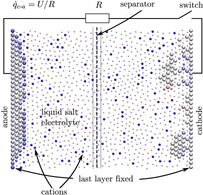
Figure 1: Color online. Illustration of a setup with 1194 atoms. Charge is encoded in the coloring, blue meaning positive charge and red negative charge. For visual distinction, electrolyte particles are chosen smallest, independent of their LJ radii, and their charge coloring is halved. The medium-sized particles are cations, while the largest particles are metallic atoms. The separator keeps non-electrolyte atoms from moving between the two half-cells. A resistive external load $R$ (following Ohm’s law) completes the circuit.

III.1 Initial setup and equilibration

We briefly describe the initial configuration of our default setup, and the start of a simulation.

• We work in a two-dimensional configuration, to reduce the computational costs associated with large particle numbers. We do not apply periodic boundary conditions: our finite system is confined by fixed walls on all sides.

• Our default system contains 358 atoms overall. We have also carried out simulations with roughly double and quadruple that number.

• Of the total number of atoms, 118 are electrode atoms. Of those, half are attached to the anode and are arranged in an hexagonal lattice with three (up to five, in larger simulations) layers. Only 20 atoms are connected to the cathode in one layer, another 39 ionized cathode atoms are dissolved in the electrolyte. This represents a crude approximation to solubility equilibrium. In a historic Voltaic cell, the dissolved particles would be Cu²⁺ ions.

• The electrolyte is distributed spatially randomly in the two half cells, under the constraint that each side is initially electrically neutral.

• We choose our MD time steps such that we sample a typical thermal oscillation of an atom with $\approx 20$ steps.

• Initially, we allow the electrolyte to equilibrate in each half-cell, barring all atoms from passing the separator. During this stage, the electrode particles are held stationary, and no ICTs/ICTMs are carried out.

• After $5,000$ MD time steps, the electrolyte has assumed a liquid glass-like state. We insert the separator instead of the impassable wall between the two half-cells, and allow both ICTs and ICTMs.

• We equilibrate for another $10,000$ MD time steps with all electrolyte atoms free to move, but damped at $\gamma\Delta t=1/60$, a factor $10$ more strongly than our default value.

• Finally, the electrode atoms are released, and the damping is set to its normal, low value. Only the last row of each electrode remains fixed in place. This limits the amount of charge transferable to roughly 66% of the electrode.

• We measure during the following $\approx 10^{7}$ MD steps.

III.2 Separator

In order to isolate the two half-cells of our battery, a simple model of a separator is inserted. In Galvanic cells, this component (called “salt bridge” in that context) is a membrane often made of filter paper, or consists of a U-shaped glass tube filled with (possibly gelified) inert electrolyte.Linden and Reddy (2010) It allows ionic species to pass through, and thus to complete the circuit with the external resistor, but prevents intermixing of dissolved electrode ions, which is often undesired.

In a present-day, commercial batteries, the two half cells are kept apart by a solid separator which is permeated by the electrolyte. In the ideal case, no electrons are allowed to pass through, but the ion conductivity is large. The separator also needs to be mechanically resistant to abuse, chemically stable in a concentrated alkaline environment (for alkaline batteries), as well as not participating in redox reactions that occur in the cell.Linden and Reddy (2010)

We implement a mathematical separator such that dissolved electrode atoms and ions feel a repulsive force when they approach the barrier, but electrolyte particles are unaffected (in our model they carry charge, and can complete the circuit). If electrode particles were allowed to mix, they could exchange split charges and form salts, or even adsorb to the opposing electrode and thus create a short circuit.

Notice that the energy barrier posed by the separator is not infinitely high. As a thermally-activated process that occurs with a probability of $\exp\left(-E_{\mathrm{sep}}/k_{\mathrm{B}}T\right)$, individual ions are expected to still pass the barrier. We choose the separator’s repulsive energy $\equiv 4$ in dimensionless units ($\approx 0.6~{}\mathrm{eV}$). This means that an ion sitting at the separator has a probability to pass through of $\approx 4.5\times 10^{-5}$ at our default temperature.

Our separator is a crude idealization of its real-world counterpart, even though their properties are similar. In a more realistic and properly parameterized simulation, the separator is a crucial component in its own right, and needs to be implemented carefully.

III.3 External circuit

One atom of the fixed layer on each electrode is chosen as the connecting point of the “wire” to connect to the opposite electrode through an external resistor. We refer to those atoms as “front atoms.” They serve as endpoints for the dedicated split charge that models the external resistor. We investigate several different modes of operation of the external circuit:

1. switch open, no electrical connection. The “external split charge” is constant. This mode is used for equilibration runs, as well as for aging tests of our battery.

2. switch closed, constant resistance, discharging. In this case, the current is determined by the instantaneous difference in chemical potential (i.e., the voltage) between the electrodes, divided by a fixed resistance. Initially, the voltage is approximately given by the difference of the electrode’s electronegativities, modified by the electric field effected by the instantaneous charge distribution. If charge transfer continued in this manner indefinitely, the transferred charge would set up an opposing electric field after some time, resisting further charge transfer. However, this electric field causes a charge separation in the electrolyte, and ions rearrange to compensate it. Recall that the separator allows free exchange of electrolyte particles across the half cells. There still is a charge buildup in the electrodes, making it energetically favorable for the electrodes to shed some of that charge. This is achieved by oxidizing surface atoms on the anode, and releasing them into the solution. Analogously, at the cathode ions dissolved in the electrolyte adsorbing to the surface are reduced. This way, the electrodes are neutral again, and the voltage returns (or approaches) that of the initial state. This process ends when there are no further ions to be dissolved (and/or adsorbed).

3. switch closed, constant resistance, charging. This is the same setting as in the discharge case, except that we add an external voltage opposing (and overpowering) the discharge voltage. We investigate to which extent the electrodes return to their previous state, and observe the battery’s hysteresis. This allows to study, for instance, surface passivation.

4. constant power or constant current. For brevity, we only present data for discharge under constant resistance, and not under constant power or constant current, even though it is possible to model those discharge modes as well. The constant power mode is a good approximation to numerous real-world applications, as many electronic devices need a minimum power throughput to function properly. In the constant current mode, charge can continue to flow even beyond the point when the voltage drops to zero. At that point the anode and cathode reverse their roles. This setting allows studying of over-discharging behavior achievable when multiple batteries with differing remaining capacities are connected in series. In that case, the voltage of the cells that still have capacity remaining can drive the empty ones into pole reversal.

III.4 Unit system and parameters

Table 1: Normalized model parameters in our default system.^$\dagger$

atom type	$\chi$	$\kappa$	description	base charge
$1$	$-4$	$4$	anode atom	0
$2$	$4$	$4$	cathode atom	0
$3$	$-4$	$4$	anode cation	+1
$4$	$4$	$4$	cathode cation	+1
$5$	$1$	$4$	electrolyte cation	+1
$6$	$1$	$4$	electrolyte anion	-1
bond type	$\varepsilon_{\mathrm{LJ}}$	$\sigma_{\mathrm{LJ}}$	$\kappa^{(0)}_{ij}$$\ddagger$
$(1,2)-(1,2)$	$1.75$	$1.0$	$3.0$
$(1,2)-(3,4)$	$1.0$	$1.0$	$3.0$
$(1,2)-(5,6)$	$1.0$	$1.0$
$(3,4)-(3,4)$	$0.75$	$1.0$	$3.0$
$(3,4)-(5,6)$	$2.0$	$1.0$
$(5)-(5)$	$0.5$	$1.0$
$(5)-(6)$	$0.5$	$1.2$
$(6)-(6)$	$0.5$	$1.0$

^$\dagger$ see Sec. III.4 for details on the normalization used. ^$\ddagger$ The parameter $\kappa^{(0)}_{ij}$ is explained in Sec. II.1. Electrolyte (solvent) atoms do not exchange partial charges in our model, neither among themselves nor with other species, and therefore those bonds do not have a $\kappa^{(0)}_{ij}$ assigned to them.

Throughout this work we use dimensionless parameters. In order to facilitate the interpretation of the presented data, this section provides ballpark estimates for representative values of real materials.

The unit of charge can be associated with the elementary charge $\left[Q\right]=1.6\times 10^{-19}~{}\mathrm{C}$. For the unit of length, we choose $\left[l\right]=2.3~{}\mathrm{\AA}$. This is to approximate the Lennard-Jones parameter $\sigma_{\mathrm{LJ}}$ used for Cu-Cu interactions in the literature.Hwang, Kwon, and Kang (2004) The value for Zn is comparable in magnitude albeit slightly larger. We define the unit of mass as the atomic mass of copper, $\left[m\right]\approx 64~{}\mathrm{amu}$. As last independent unit, the energy is normalized to $\left[E\right]=0.16~{}\mathrm{eV}\approx 15.5~{}\mathrm{kJ/mol}$. Again, this is so that the interaction between metallic electrode particles is comparable to values for $\epsilon_{\mathrm{LJ}}$(Cu-Cu) in the literature.

Together, length, charge, energy, and mass specify a complete set of units for our purposes. Derived units are the unit of current $\left[I\right]\approx 350~{}\mathrm{nA}$, $\left[R\right]\approx 3.3\times 10^{5}~{}\mathrm{\Omega}$ as resistance normalization, $\left[U\right]\approx 160~{}\mathrm{mV}$ as unit of voltage, and $\left[t\right]\approx 0.5~{}\mathrm{ps}$ as unit of time. Our battery demonstrator operates at a temperature $T\approx 740~{}\mathrm{K}$, comparable to a liquid-salt battery.Bradwell et al. (2012)

With these choices of units, the default value for the electronegativity difference between anode and cathode is $\Delta\chi=1.28$ V, which is close to many standard cells, e.g., alkaline (1.5 V) or NiMH (1.2 V) batteries. In the default parameterization, we use atomic hardnesses of $\kappa=0.64$ eV, which is much smaller than typical values, e.g., $\kappa_{\rm Cu}=7.3$ V/e and $\kappa_{\rm Li}=4.7$ V/e.Ghosh and Islam (2010) Moreover, unlike real systems, our standard values for $\chi$ and $\kappa$ do not reproduce a neutral dissociation limit of dimers, because $\kappa/2-\chi>0$, as can be seen from Eq. (2). We made this choice of parameters to accelerate the generation of ions. At the same time, we ensured in selected simulations that the qualitative features of the discharge curves remained unchanged for much larger values of $\kappa$ and smaller values for $\chi$ (see Sec. IV).

In order to compare our results with macroscopic systems, our model battery would have to be scaled up by a factor of roughly $10^{21}$. In principle, each spatial dimension can have a different scaling factor, however, for simplicity, one may assume the same factor of $10^{7}$ in each direction. An inherent ambiguity of how to scale the direction normal to the interfaces remains. One way to scale the simulation is to take our nano-battery as an electrical element and connect $10^{7}$ of them in series, and $10^{14}$ in parallel. This method yields an overall open-circuit voltage (OCV) of $12.8~{}\mathrm{MV}$ for our default choice of parameters ($\Delta\chi=8$). Connecting the external resistors in a similar fashion as the batteries leads to a scaled resistance of $66~{}\mathrm{\Omega}$ (microscopic system: $R=2000$ in dimensionless units). Consequently, the nominal macroscopic discharge current would be $70$ kA. Discharge now takes $10^{7}$ times longer (about $0.1$ s) than in the microscopic case, because the total number of transferrable charges increases by $10^{21}$, while the current only increases by $10^{14}$.

Alternatively, one can scale both battery and resistor as a whole in each spatial dimension. This way one retains the value for the macroscopic resistance of $66~{}\mathrm{\Omega}$. In contrast, the voltage in this case still has its microscopic value of $1.28~{}\mathrm{V}$. The resulting nominal macroscopic discharge current is $7$ mA, which is not very much lower than real-world currents. Now the discharge would take $10^{14}$ times longer than in our microscopic model (about 14 d). We stress that the discharge characteristics of such a scaled-up version of our model battery would be different from the ones presented in this work because the electrode surface-to-volume ratio would be much reduced in the macroscopic battery, among other reasons.

In many figures we show discharge curves, i.e., plots showing the instantaneous voltage vs. the transferred relative charge. In those plots, the voltage is normalized by the electrode atom’s difference in electronegativities, because that is the difference in chemical potential in absense of any charge effects or electric fields. The transferred relative charge is the total charge flown across the external resistor, normalized by the total number of atoms in either of the electrodes. We consider not only the dissolvable layers but also the fixed electrode atoms. Each atom can change its oxidation state by one: the mobile layers can desorb as cations, while the fixed layer’s charge is balanced through the formation of a double layer from the electrolyte. Note that the charge through the external resistor is fractional because we implement it as a dedicated (and not-equilibrated) split charge. We chose to do this instead of sending across only integer increments in order to get smooth curves. This can be considered in implicit average over many time steps.

III.5 Limitations and code efficiency

At this stage, our model only contains some rudimentary approximation to chemistry, and the ability to model redox reactions. We only consider two-body forces, and leave dihedral and torsional interactions for future work. Moreover, at short distances we do not screen the Coulomb interaction, even though the wave functions of atoms overlap in such a situation, and the point-charge approximation breaks down.

Our current implementation can be made to run much more efficiently. Particular points to note are the following. We do not cut off the Lennard-Jones interaction, which makes its complexity $\mathcal{O}(N^{2})$. We also compute the Coulomb interactions with an expensive $\mathcal{O}(N^{2})$ direct-sum algorithm, which limits the system sizes we can currently study. We could save computing time with a more efficient approach. We plan an implementation into the open-source code LAMMPS, which will alleviate this limitation.

Even with such improvements the solution of the large linear system is more expensive than the setup of the system matrix, for which the Coulomb term is calculated. Two ways to make this cheaper come to mind: the first is to use a more efficient algorithm for the solution of the linear system, for example using a conjugate gradient method.Press et al. (2007) Second, we could update only the split charge in vicinity of the ICT. At this developmental stage, we re-equilibrate all partial charges after an ICT. Instead, one could implicate only the partial charges within some cutoff radius $R^{\mathrm{opt}}$. This would mean introducing a finite signal speed for the SQE, as a split charge could be transferred a certain distance in one time step. The instantaneousness of the update would be lost, making it harder to model metals. The advantage is that it would make the operation $\mathcal{O}(N)$ instead of $\mathcal{O}(N^{2})$. The resulting error can be estimated and is bounded: the change in the split charges, and thus the error as a result of restricting the update distance, drops off exponentially with increasing cutoff distance.Nistor and Müser (2009)

Lastly, in future implementations we will randomize the order of bonds for which we attempt an ICT and for which an ICTM is carried out, and eliminate the slight ordering bias currently present in the code.

All of the optimizations described above are left for future work; even without them (albeit for small systems) the method yields encouraging results.

IV Results

In this section we describe the results gleaned from our simulations. We emphasize again that our model is more a proof-of-concept rather than a faithful representation of a real battery. As such, the parameters have not been chosen appropriate for any specific material. Our intent is to demonstrate that redoxSQE nevertheless reproduces generic properties of macroscopic batteries without further input.

The model necessarily has a number of parameters, albeit not nearly as many as some mesoscopic porous electrode simulations.Menzel, Willkomm, and Wolisz (2011) Some are microphysical and chemical parameters, for instance the LJ properties of the materials, the atomic hardness, or the electronegativities. Those are in principle readily parameterizable or even measurable quantities for real materials, but we elect to use representative values (see Sec. III.4), rather than to model specific materials. The parameters associated with the bond hardness are not as easily measured, but can in principle be fit to values found from measurements and ab initio quantum-chemical DFT simulations, such as ESP (electrostatic potential) partial charges, Hirshfeld-I charges, and dipole moments of molecules.Nistor et al. (2006); Mathieu (2007); Verstraelen, Van Speybroeck, and Waroquier (2009) Other parameters are implementation choices such as number of atoms to model, the electrode setup, and the geometry of our cell. Finally, we vary parameters that have a documented and experimentally accessible impact on battery performance, such as the temperature, and whether the battery is discharged continuously or in pulses. The dependence on this last set of parameters results naturally and self-consistently with our method, and does not have to be put in implicitly or explicitly.

IV.1 Dependence on internal model parameters

In this section, we explore the dependence of the discharge characteristics on internal model parameters, while Sec. IV.2 focuses on external parameters. In SQE, the difference in electronegativity between atoms of two metals determines the open-circuit voltage (OCV). In all following plots, the voltage is normalized to this value.

Separating a diatomic molecule adiabatically results in neutral products for each pair of stable elements. However, if $\Delta\chi>(\kappa_{1}+\kappa_{2})/2$, it is energetically favorable that negative integer charge (i.e., an electron) remains on the more electronegative partner.Müser (2012) For a multi-atom system, the expression for the neutral dissociation limit is not as simple anymore, because the atomic hardness is reduced in an ensemble.Müser (2012) In our default system, we choose $\chi=\pm 4$ and $\kappa=4$, in order to facilitate the formation of ions at the anode, even though these values lead to a violation of the neutral diatomic dissociation limit. However, Fig. 2 shows that this does not have a large impact on the discharge curve: even for $\chi=\pm 1.9$ and $\kappa=4$, satisfying the neutral dissociation limit, the qualitative picture remains.

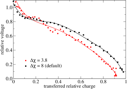
Figure 2: Color online. Discharge curves of our battery demonstrator for different electronegativities. The data represents an average over several independent runs, and each point is averaged over many MD time steps. The solid lines are inserted to guide the eye. Our default model has $\chi=\pm 4$ and $\kappa=4$ which violates the dissociation limit: dissociating a diatomic molecule will produce ionic instead of neutral products. The runs with $\chi=\pm 1.9$ do not have this flaw, and still exhibit similar discharge behavior, even though the likelihood of anode atoms to dissolve as ions is reduced. The scatter is larger for smaller $\chi$ since the theoretical voltage is reduced by a factor of $2.1$, and thus the signal-to-noise ratio halves, even though in this case we average over 8 different realizations.

We note that the large scatter stems from the small number of atoms in our simulations. If we dissolve $50\%$ of the total number of anode atoms, we have 30 cations in solution, and a statistical uncertainty of $\mathcal{O}\left(1/\sqrt{30}\right)$, i.e., $\approx 15\%$. The stochastic error reduces by a factor of two by averaging over 4 independent realizations.

In Sec. III.4 we reported representative values as normalization for the dimensionless parameters used in this work, and noted that our standard value for the atomic hardness $\kappa$ was rather low compared with values for real materials. In Fig. 3, we show the discharge behavior of our nano-battery for $\kappa=10$ and $\Delta\chi=8$, again satisfying the neutral diatomic dissociation limit. In this case, ion formation (i.e., redox reactions at the electrode surface) takes much longer, and the external resistor needs to be scaled up in order to get similar behavior. A factor of 2.5 in $\kappa$ is approximately compensated by a factor of 25 in resistance. In addition, the plateau is far less pronounced for the larger $\kappa$, and the discharge proceeds faster. Note that the initial voltage in this case is also higher. The reason is that some pre-dissolved cations adsorb to the electrode immediately, and cause a greater difference in chemical potential, and therefore OCV. In order to have the curves overlap for better visual comparability, we scaled down the results for $\kappa=10$ by a factor of 1.3, which compensates for the larger OCV. Note that the simulation with $R=50,000$ and $\kappa=10$ takes very long, for the reasons described above, and was terminated before all charge was transferred.

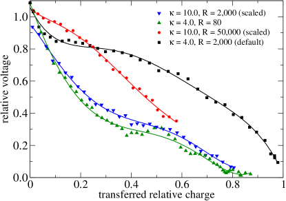
Figure 3: Color online. Discharge curves of our battery demonstrator varying the atomic hardness. The data represents an average over 4 independent runs, and each point is averaged over many MD time steps. The solid lines are inserted to guide the eye. Runs with $\kappa=10$ (approximating real atomic hardnesses more closely than our standard value) require much higher external resistances in order to achieve similar discharge behavior as for the default value of $\kappa$. For larger values, the plateau is much less pronounced. The $\kappa=10$ runs are scaled down by a factor of 1.3 so that they overlap the $\kappa=4$ curves better (see text).

In Fig. 4, we exemplify the influence of the LJ parameters on the discharge curve. We vary $\varepsilon_{\mathrm{LJ}}$ between electrode ions and the electrolyte. A higher value means that it is favorable for an ion to surround itself with electrolyte atoms, as opposed to other atoms with which its $\varepsilon_{\mathrm{LJ}}$ is lower. The discharge curve has a higher and more extended plateau for a smaller $\varepsilon_{\mathrm{LJ}}$, caused by the reaction on the cathode, where a lower value means that it is more likely that an ion is adsorbed to the electrode. At the anode, the opposite should be the case. There, a greater $\varepsilon_{\mathrm{LJ}}$ should make it more likely for an ion to be dissolved into the electrolyte. However, the test case with $\varepsilon_{\mathrm{LJ}}^{\mathrm{anode}}>\varepsilon_{\mathrm{LJ}}^{\mathrm{cathode}}$ changes the plateau only marginally. We conclude that the cathode reaction is more important in this respect. If the method in implemented into more sophisticated software (e.g., LAMMPS), it can be used with more realistic force fields for particle-particle interactions than what is used herein (i.e., simple two-particle LJ interaction).

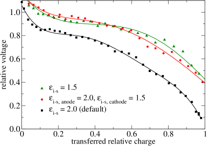
Figure 4: Color online. Discharge curves of our battery demonstrator varying the LJ parameter $\varepsilon_{\mathrm{LJ}}$ between electrode ions and the solvent (electrolyte). The data represents an average over 4 independent runs, and each point is averaged over many MD time steps. The solid lines are inserted to guide the eye. This figure exemplifies the optimization potential that lies in picking optimal materials for the battery: a smaller affinity between electrolyte and cations boosts battery performance significantly. The anode half-cell reaction seems less important in this respect, as optimizing it does not yield a comparable additional improvement.

While the LJ parameters in principle can be deduced from experiments, pinning down the parameterization details of the bond hardness so that they match experiments or ab initio results is harder to accomplish. Nistor et al. (2006); Mathieu (2007); Verstraelen, Van Speybroeck, and Waroquier (2009) Fortunately, those parameters do not affect the results very strongly, as evidenced in Fig. 5. A change by $50\%$ in the cutoffs for $\kappa_{ij}^{(\mathrm{b})}$, given in Eq. (7), does not make a big difference: all curves nearly overlap with those of our default model in the practically relevant regime (until a discharge of $\gtrsim 60\%$). In Fig. 6 we scale the parameter $\kappa_{ij}^{(0)}$ up and down by a factor of $3$. The results do not depend sensitively on this choice, either. These results indicate that the detailed form of $\kappa_{ij}^{(\mathrm{b})}$ is not of great importance. The only criterion is that the next-nearest neighbor should not be connected with a dielectric bond. This translates into the “long” cutoff $r_{\mathrm{l}}$ be substantially smaller than the distance to the next-nearest neighbors. Otherwise a great number of additional ICTs will be attempted. This does not change the result, either, but the computations will be slowed down tremendously. The simulation shown by the yellow curve in Fig. 5 shows this case, and we terminated it before all charge had transferred.

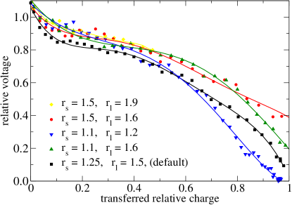
Figure 5: Color online. Discharge curves of our battery demonstrator for various cutoffs in the parameterizations of the bond hardness. The data represents an average over 4 independent runs, and each point is averaged over many MD time steps. The solid lines are inserted to guide the eye. A change in the cutoffs entering $\kappa_{ij}^{(\mathrm{b})}$ by $50\%$ does not significantly alter the results: all curves resemble our default model. This indicates that the detailed form of $\kappa_{ij}^{(\mathrm{b})}$ is not of great importance.

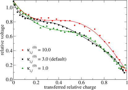
Figure 6: Color online. Discharge curves of our battery demonstrator for different parameterizations of $\kappa_{ij}^{(\mathrm{b})}$. The data represents an average over 4 independent runs, and each point is averaged over many MD time steps. The solid lines are inserted to guide the eye. We vary the parameter $\kappa_{ij}^{(0)}$ by a factor of $3$ to greater and smaller values. The results do not depend sensitively on this choice.

We tested the effect of various other simulation parameters. For brevity we only describe the results without including additional figures.

• We increased the damping by a factor of 10 without observing any qualitative nor quantitative changes in the discharge behavior. This means that the Langevin damping only has the desired effect to limit the battery heating up as a consequence of energy release, but is not strong enough to influence the dynamics much.

• A variation in the LJ parameters between electrode metals and their ions by $50\%$ also did not alter the characteristics significantly. Our choice stems from the idea that ions are bound less tight to the electrodes than neutral metal atoms. This again aids the release of cations into solution.

• We modified the relative importance of the different contributions to the potential energy. A decrease of the effect of the Coulomb energy by up to $33\%$ (and thereby a corresponding increase in relative importance of the other effects) did not influence the discharge curve qualitatively.

• Similarly, neither scaling the battery in one direction, nor doubling the amount of electrolyte without adding more electrode atoms, nor changing the electrode surface area modifieded the results significantly. We conclude that we are not hampered by a lack of electrolyte. However, reducing the number of electrolyte atoms to half its default value will limit the number of ions that can be dissolved, and deteriorate our battery demonstrator’s performance.

IV.2 Dependence on external factors, rates and aging

An ideal battery should retain its theoretical voltage until the active material has been used up, that is, until the anode is completely dissolved, or all free cations have been reduced and adsorbed at the cathode surface. Only at this point should the voltage drop to zero.Linden and Reddy (2010) In reality, batteries have an internal resistance, and both the electrolyte and the electrode are polarizable. The former reduces the actual voltage drop across the battery, while the latter is responsible for forming Helmholtz double layers at the electrode surfaces, and thus depleting some of the battery’s capacity. Such effects cause both the actual working voltage as well as the usable capacity to be reduced from their theoretical limits. Additionally, a battery’s voltage also depends on the discharge current, such that a higher discharge current will decrease the discharge voltage. In Fig. 7 we show curves demonstrating this behavior. At high external resistance (i.e., low discharge current), the voltage stabilizes at $\lesssim 90\%$ of its theoretical voltage until about $70\%$ of the available charge has been transferred, at which point it drops quickly. At medium resistance (our default model), the voltage does not feature such a pronounced plateau, but still has $\approx 60\%$ of its voltage at $60\%$ discharge. In contrast, the voltage for a discharge at high currents decreases much more steeply. These curves are reminiscent of those presented in Refs. Doyle et al. (1996); Srinivasan and Newman (2004); Wang and Sastry (2007); Linden and Reddy (2010), the discharge curves of Panasonic’s zinc carbon batteries,Panasonic Corporation (2009) and those of Duracell’s alkaline batteries.Procter & Gamble (2012)

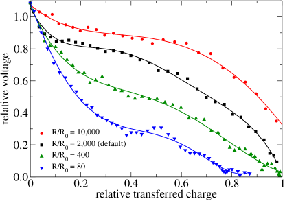
Figure 7: Color online. Discharge curves of our battery demonstrator with different external resistors. The data represents an average over 4 independent runs, and each point is averaged over many MD time steps. The solid lines are inserted to guide the eye. The higher the external resistance, the closer the battery’s behavior approaches the theoretical discharge curve. In this property, and the shape of the discharge curve, our nano-battery resembles a macroscopic battery. Initially, the voltage declines sharply, as the electrodes are charged before ions are dissolved or adsorbed, respectively. This is followed by an extended plateau when the voltage stays constant as the charge transfer through the external resistance is balanced by an equal amount of ion transfer in the electrolyte. At the same time, additional charge on the electrodes is now compensated by dissolving and adsorbing ions. Finally, another steep decline concludes the discharge, as the electrodes are consumed and their surfaces passivated.

If the internal resistance of a battery exceeds the external resistance, we effectively have a short circuit, and the battery will discharge as a capacitor, with an initial exponential decay of the voltage.

A factor that is of crucial importance to real batteries is the temperature at which they operate. Electric vehicles need to be able to reliably operate at temperatures ranging from $\lesssim-30^{\circ}~{}\mathrm{C}$ all the way to $\gtrsim 50^{\circ}~{}\mathrm{C}$. However, low temperatures decrease both the actual voltage as well as the battery’s capacity.Linden and Reddy (2010) Figure 8 shows the temperature dependence of our battery demonstrator. As in macroscopic batteries, the voltage is closer to the theoretical voltage for high temperatures, while it is significantly reduced for lower temperatures. The battery’s capacity — the area under the curve — decreases by $\approx 42\%$ if the temperature is lowered by $25\%$, and increases by $\approx 46\%$ if the temperature is raised by $50\%$ from our default temperature. We note that our temperature of $T=740~{}\mathrm{K}$ is quite large, comparable to liquid-salt batteries,Bradwell et al. (2012) but greatly exceeds room-temperature. However, we once more emphasize the qualitative nature of our findings, not their realism.

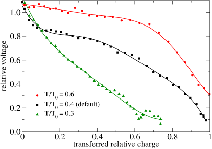
Figure 8: Color online. Discharge curves for different system temperatures. The data represents an average over 4 independent runs, and each point is averaged over many MD time steps. The solid lines are inserted to guide the eye. At lower temperatures ($T\approx 550~{}\mathrm{K}$), the battery’s performance deteriorates dramatically, while it improves at a higher temperature ($T\approx 1,100~{}\mathrm{K}$).

In Fig. 9 we present aging studies of our model battery. It is common in some electronic devices to intersperse recuperation periods with discharge periods. During this time, polarization effects are reduced and some of the initial voltage can be recovered.Linden and Reddy (2010) In order to examine the effects of intermittent discharge on our model battery, we discharge it until a certain amount of current has been drained, and then open the switch and let the system age. Were it an electrochemical capacitor, no recovery of voltage would be expected. However, we see a nearly full recuperation of the initial voltage (with some fluctuations). This voltage is held for $\approx 10^{7}$ time steps. After some time, ions manage to pass through the separator (which is a thermally activated process, see Sec. III.2). This causes a voltage drop that contributes to self-discharge. In a macroscopic battery this process will not take place as quickly as in our nanoscale device, but one mechanism for is elucidated in our model. The use of redoxSQE furthermore allows us to study the morphology changes that the electrodes have undergone, how much surface material is passivated and other microphysical parameters of interest.

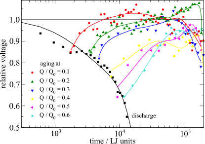
Figure 9: Color online. Aging studies of our model battery. The data represents an average over 4 independent runs, and each point is averaged over many MD time steps. The solid lines are inserted to guide the eye. After a certain amount of charge has flown through the resistor, the switch is opened and the relaxation observed. In all cases, the voltage recuperates to almost the nominal value (with fluctuations). This behavior would not be present in a capacitor, which does not recover its charge after the circuit is broken. After a certain time, ions pass the separator and cause self-discharge, which gives rise to a voltage drop.

All reactions occurring in our system are micro-reversible, therefore our nano-battery is a secondary, rechargeable cell. Figure 10 shows what happens if we recharge our battery demonstrator. We discharge our default system at the default constant resistance ($R=2000$). After $\approx 60\%$ of the total capacity (35 out of 59 integer charges) have been transferred through the external circuit, a charging current is switched on, in opposite direction as the discharge current. We choose its magnitude approximately three times the “average” discharge current (averaged over the complete discharge of the same model).

We consider two cases: in the first, the charging current is switched off again when the voltage reaches $\approx 1.1$ times the OCV. In this case, the discharge curve in the second cycle has deteriorated compared with the initial discharge; the battery has degraded. The reason is that the electrodes do not fully return to their initial state during the charging, but merely the electrolyte reconfigures to balance the dissolved cations in either half cell. If one were to let the system relax after charging, some dissolved cations would return to the anode, and some material deposited on the cathode would also dissolve again. A realistic all-atom simulation using redoxSQE can be useful in the investigation of dendrite formation in this process which can short-out and destroy Li-ion batteries.Tarascon and Armand (2001); Armand and Tarascon (2008); Bhattacharyya et al. (2010) It could also help to study the cycling behavior of batteries, and their degradation.

In the second case, all charge is transferred back. Then, the voltage is much higher than the initial OCV. This behavior is also seen in real batteries,Linden and Reddy (2010) and stems from a buildup of a polarization layer opposite that which forms during discharge. In this case, the second discharge is not very dissimilar from the first one.

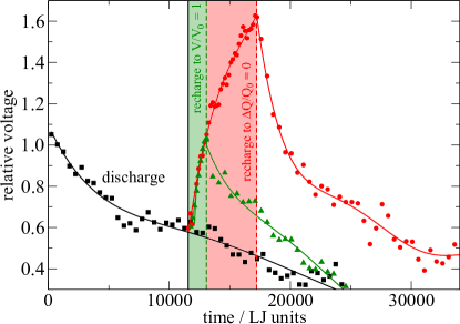
Figure 10: Color online. Discharge and recharge curves of our battery demonstrator. The lines are inserted to guide the eye. Our default system is discharged (black squares) at constant resistance, until $\approx 60\%$ of the total charge has been transferred through the external resistor. At this point, a constant external charging current is switched on; its magnitude is chosen approximately three times the (average) discharge current. This charging current is switched off again when the voltage reaches the OCV (middle, green triangles), or when all charge has been transferred back (top, red circles). In the latter case, the voltage is much higher than the initial OCV.

V Discussion and conclusions

In this work, we demonstrated that the redoxSQE method Müser (2012) can model redox reactions in an atomistic molecular dynamics setting, and used it to simulate a nanoscale battery demonstrator. Even though we did not use a parameterization describing any real energy materials, we reproduced generic discharge curves of macroscopic batteries. For example, lower operating temperatures reduce the effective capacity of a battery. Higher discharge rates have the same effect, but the voltage recuperates when the battery is aged (e.g., discharged in pulses). Upon recharging, the battery performance degrades slightly, and the electrode surface morphology changes during the battery’s operation.

Some internal model parameters are not fully accessible experimentally, such as the bond hardness, which is an ad-hoc parameter arrived at in a top-down fashion, by describing the bond-breaking behavior. In a theoretical work, Verstraelen et al. Verstraelen et al. (2013) connect the bond hardness to parameters computed with atom-condensed DFT, i.e., derive it in a bottom-up fashion, and may help to motivate this parameter and ascertain its value quantitatively. We showed that, for the battery demonstrator, the results neither depend strongly on the detailed implementation, nor on the precise value of the bond hardness.

The atomic hardness plays an important role in determining the time scales of ion formation at the electrode interface, and thus determines partly the internal resistance of the battery, while the electronegativity difference sets the open-circuit voltage. But changing those two parameters does not alter the qualitative discharge picture. Rather, the battery’s behavior is predominantly defined by external quantities such as temperature, rates of discharge. We obtain results similar to the intermittent discharge mode,Linden and Reddy (2010) and see self-discharge when the battery is aged too long.

In a recent previous paper we applied the same technique to case studies in contact electrification between two clusters of ideal metals and ideal dielectrics, respectively, showcasing its ability to simulate history-dependence.Dapp and Müser (2013) RedoxSQE reproduces charge hysteresis effects during approach and retraction.

One shortcoming of our current implementation is that the electrolyte is modeled with fixed-charge particles that do not participate in split charge exchange, nor in ICTs. It is an ideal insulator for electrons, and the lack of electronic conduction leaves only penetration of the separator by ions as self-discharge mechanism. This idealization will be abandoned in future work.

Further development effort will need to be expended on optimizing the method (see Sec. III.1, and Ref. Müser (2012)) to make multi-million atom simulations possible. An implementation into LAMMPS is planned. In order to simulate specific materials or battery setups (such as alkaline batteries, or Li-ion rechargeables), much chemically-specific parameterization will need to be done.Nistor et al. (2006); Mathieu (2007); Verstraelen, Van Speybroeck, and Waroquier (2009); Verstraelen et al. (2012) Furthermore, more realistic empirical many-body force fields are necessary for realistic all-atom simulations. We point out that the model in its current implementation can best describe non-directed interactions, as they are prevalent for instance in Alkali batteries, with their isotropic reactions of s-orbitals.

Notwithstanding those necessary improvements, it is encouraging that the method already reproduces generic features of batteries. Mesoscale battery models require many assumptions and intimate knowledge of the materials in question, and cannot answer fundamental microphysical questions. DFT/MD methods, on the other hand, have been used for highly detailed and isolated problem aspects, but need to stay away from the electrode-electrolyte interface where redox reactions take place. Arguably, this is the most interesting region, as it determines not only the ultimate cell performance, but also is where cell degradation takes place. Harris et al. Harris et al. (2010) write “the ability to predict cell degradation remains a challenge because so many unaccounted for and seemingly unrelated micro-scale degradation mechanisms have been identified or postulated. […] Without … theoretical analysis, cause-and-effect relationships between observation and degradation pathway can be difficult to demonstrate.” RedoxSQE is a first step toward filling this gap. It allows to model all aspects of a (microscopic) battery in one simulation, and gather insights into the processes happening at the electrode-electrolyte interface.

Besides modeling an entire all-atom battery, redoxSQE could also serve as part of hybrid multiscale schemes, where bulk phenomena inside an electrode or within the electrolyte are computed with a mesoscopic model while the electrochemical activity is tackled by redoxSQE.

Daniel’s Handbook of Battery Materials Daniel and Besenhard (2011) states as requirement for a generic life estimation model that it “must relate the measured cell performance at any given time to a combination of … effects.” In conjunction with a more realistic force field and with a proper parameterization of the materials, redoxSQE holds promise to enable the study of battery degradation and the optimization of battery performance.