The VLT-FLAMES Tarantula Survey

Abstract

Aims. We compile the first comprehensive census of hot luminous stars in the 30 Doradus (30 Dor) star forming region of the Large Magellanic Cloud. We investigate the stellar content and spectroscopic completeness of early type stars within a 10arcmin (150pc) radius of the central cluster, R136. Estimates were made of the integrated ionising luminosity and stellar wind luminosity. These values were used to re-assess the star formation rate (SFR) of the region and determine the ionising photon escape fraction.

Methods. Stars were selected photometrically and combined with the latest spectral classifications. Stellar calibrations and models were applied to obtain physical parameters and wind properties. Their integrated properties were then compared to global observations from ultra-violet (UV) to far-infrared (FIR) imaging as well as the population synthesis code, Starburst99.

Results. The census identified 1145 candidate hot luminous stars of which $>700$ were considered genuine early type stars that contribute to feedback. We assess the spectroscopic completeness to reach 85% in outer regions ($>5$ pc) but fall to 35% in the vicinity of R136, giving a total of 500 hot luminous stars with spectroscopy. Only 31 W-R and Of/WN stars were included, but their contribution to the integrated ionising luminosity and wind luminosity was $\sim 40$% and $\sim 50$%, respectively. Similarly, stars with $M_{\rm{init}}>100\,\mathrm{M}_{\odot}$ (mostly H-rich WN stars) also showed high contributions to the global feedback, $\sim 25$% in both cases. Such massive stars are not accounted for by the current Starburst99 code, which was found to underestimate the integrated ionising luminosity and wind luminosity of R136 by a factor $\sim 2$ and $\sim 9$, respectively. The census inferred a SFR for 30 Dor of $0.073\pm 0.04$ M_⊙ yr^-1. This was generally higher than that obtained from some popular SFR calibrations but still showed good consistency with the far-UV luminosity tracer and the combined H$\alpha$ and mid-infrared tracer, but only after correcting for H$\alpha$ extinction. The global ionising output was also found to exceed that measured from the associated gas and dust, suggesting that $\sim 6^{+55}_{-6}$% of the ionising photons escape the region.

Conclusions. When studying the most luminous star forming regions, it is essential to include their most massive stars if one is to determine a reliable energy budget. The large ionising outputs of these stars increase the possibility of photon leakage. If 30 Dor is typical of other large star forming regions, estimates of the SFR will be underpredicted if this escape fraction is not accounted for.

1 Introduction

The Tarantula Nebula (NGC 2070, 30 Doradus - hereafter “30 Dor”) in the Large Magellanic Cloud (LMC) is optically the brightest H ii region in the Local Group (Kennicutt:1984). It has been subject to numerous ground-based photometric and spectroscopic studies, displaying an abundance of hot massive stars (Melnick:1985; SchildTestor:1992; Parker:1993; WalbornBlades:1997). Hubble Space Telescope observations later revealed their high concentration in the more crowded central cluster, R136 (Hunter:1995; MasseyHunter:1998), also believed to be the home of stars with masses $>150\,\mathrm{M}_{\odot}$ (Crowther:2010). Roughly a third of the LMC Wolf-Rayet (W-R) stars compiled in Breysacher:1999 are contained within the 30 Dor nebular region of N157 (Henize:1956), with several found within R136 itself. The stellar population of 30 Dor spans multiple ages; from areas of ongoing star formation (Brandner:2001; Walborn:2013) to older ($\sim 20-25$ Myr) supergiants in the Hodge 301 cluster (GrebelChu:2000).

More recently, the VLT-Flames Tarantula Survey (VFTS, see Evans:2011, hereafter, Paper I) has provided unprecedented multi-epoch spectroscopic coverage of the massive star population. The VFTS greatly extends our sampling of massive stars at different luminosities and temperatures, which are unobtainable from distant galaxies. In particular, it allows several topics to be assessed including: stellar multiplicity (Sana:2013a); rotational velocity distributions (Dufton:2013 & Ramírez-Agudelo et al. in prep); the dynamics of the region and R136 (Henault-Brunet:2012b). In this paper we look at 30 Dor in a broader context. Prior to the VFTS, $<20$% of massive stars within the central $10\,\mathrm{arcmin}\approx 150$ pc (adopting a distance modulus to the LMC of $18.49\pm 0.047$ mag i.e. a distance of $\approx 49.97\pm 1.11$ kpc, Pietrzynski:2013) had a known spectral type (SpT). As we will show, this spectroscopic completeness is improved to $\sim 85$% by the VFTS, enabling us to compile the first robust census of the hot luminous stars in 30 Dor.

Its close proximity and low foreground extinction, combined with its rich source of hot luminous stars, make 30 Dor the ideal laboratory for studying starburst environments in the distant universe. In more distant cases, however, stars cannot be individually resolved and starburst regions can only be studied via their integrated properties. This census provides us with a spectral inventory for an archetypal starburst, along with estimates of the stellar feedback. Here, we focus on radiative and mechanical feedback, to which hot luminous stars greatly contribute, especially prior to core-collapse supernova explosions. Their high luminosities and temperatures provide a plethora of extreme UV (EUV) photons ($Q_{\mathrm{0}}$), that ionise the surrounding gas to produce H ii regions. Meanwhile, their strong stellar winds lead to a high wind luminosity ($L_{\mathrm{SW}}$), capable of sweeping up the ISM into bubbles, even prior to the first supernovae (ChuKennicutt:1994). R136 itself, appears to show evidence of such effects through an expanding shell (e.g. vanLoon:2013).

Individual analyses are currently underway of all the VFTS early type stars, allowing determination of their parameters, along with their feedback. Here, we employ various stellar calibrations to estimate the integrated properties for the entire 30 Dor region. This allows for comparisons to the global properties of the nebula. The integrated ionising luminosity is typically obtained by observing the hydrogen recombination lines (such as H$\alpha$) or the radio continuum flux. However, not all ionising photons will necessarily ionise the surrounding gas since they may be absorbed by dust or even escape the region altogether. The star formation rate (SFR) can be determined for such regions using the inferred $Q_{\mathrm{0}}$, but an accurate SFR relies on the knowledge of the fraction of escaping ionising photons.

A similar approach to the present study has been carried out for the Carina Nebula. Smith:2006 and SmithBrooks:2007 found the integrated radio continuum flux to provide $\sim 75$% of the $Q_{\mathrm{0}}$ determined from the stellar content, suggesting a significant fraction of the photons were escaping, or were absorbed by dust. Their $Q_{\mathrm{0}}$ determined from the H$\alpha$ luminosity was even smaller, only a third of the stellar output. This was thought to arise from a large non-uniform dust extinction that had been unaccounted for. Lower luminosity H ii regions have also been studied in the LMC (OeyKennicutt:1997). Initial comparisons to the H$\alpha$ luminosity suggested 0-51% of ionising photons escape their regions and could potentially go on to ionise the diffuse warm ionised medium (WIM). However, these H ii regions were later revisited by Voges:2008 with updated atmospheric models, indicating a reduced photon escape fraction, with radiation being bound to the regions in all but 20-30% of cases.

In previous studies, the feedback of up to a few dozen stars are accounted for (70 in the Carina Nebula). 30 Dor is powered by hundreds of massive stars of various spectral types (SpTs) and the census gives an insight into their relative importance. Parker:1998 already used UV imaging to show how a few of the brightest stars make a significant contribution to the $Q_{\mathrm{0}}$ in the region. Indebetouw:2009 and Pellegrini:2010 used infrared (IR) and optical nebular emission lines, respectively, to study the ionised gas itself, with both favouring a photoionisation dominated mechanism in 30 Dor. R136 appeared to play a prominent role as nearly all bright pillars and ionisation fronts were observed to lead back to the central cluster (Pellegrini:2010). Indebetouw:2009 also noted regions of more intense and harder radiation which typically coincided with hot isolated W-R stars. OeyKennicutt:1997 and Voges:2008 omit W-R stars when studying their H ii regions, in view of uncertainties in their $Q_{\mathrm{0}}$. However, earlier work by CrowtherDessart:1998 compiled a list of the hot luminous stars in the inner 10 pc of 30 Dor and found the W-R stars to play a key role in the overall feedback. We extend their study to a larger radius, employing updated stellar calibrations and models to determine whether the W-R star contribution still remains significant.

Population synthesis codes can predict observable properties of extragalactic starbursts, and 30 Dor equally serves as a test bed for these. Direct comparisons to the stellar content and feedback in similar luminous star forming regions is relatively unstudied. The R136 cluster is believed to be at a pre-supernova age and so has largely preserved its initial mass function (IMF), although mass-loss and binary effects may have affected this to some extent. Its high mass ($M_{\rm{cl}}\lesssim 5.5\times 10^{4}\,\mathrm{M}_{\odot}$, Hunter:1995) also ensures that its upper mass function (MF) is sufficiently well populated, hence ideal to test synthetic predictions of the stellar feedback. Comparisons to the entire 30 Dor region are less straight forward given its non-coevality, but can still be made by adopting an average age for 30 Dor.

A breakdown of the present paper is as follows. In Section 2, we present the photometric catalogues used in the census, their magnitude and spatial limits. Section 3 sets out the different criteria used for selecting the hot luminous stars from the photometric data. In Section 4, we match our selected hot luminous stars with any available spectral classifications. We examine the spectroscopic completeness of the census in Section 5. Section 6 discusses the different calibrations assigned to each SpT. Section 7 brings together all of the stars in the census, considering their age and mass while Section 8 focuses on their integrated feedback and the different contributions from both the central R136 cluster and 30 Dor as a whole. Section 9 discusses the SFR of 30 Dor and its potential photon escape fraction. Section LABEL:sec:Summary discusses the impact of our results and summarises the main findings of the census.

2 Photometry

Our aim was to produce as complete a census as possible of the population of hot luminous stars in the 30 Doradus region. The first step began by obtaining a photometric list of every star in the region, from which our potential hot luminous candidates could be selected. As in Paper I, the overall list had four primary photometric catalogues: Selman, WFI, Parker and CTIO, outlined below.

The ‘Selman’ photometry (Selman:1999), with Brian Skiff’s reworked astrometry, used observations from the Superb-Seeing Imager (SUSI) on the 3.5 m New Technology Telescope (NTT) at La Silla. Data covered the central 90 arcsec of 30 Dor in the $UBV$ bands. The completeness limit was $V=19.2$ mag although sources reached fainter, with typical photometric errors spanning 0.005-0.05 mag.

The ‘WFI’ photometry was the main source of photometry used for the census, based on the same observations outlined in Section 2.1 of Paper I. $B$- and $V$-band photometry was obtained with the Wide-Field Imager (WFI) at the 2.2 m Max-Planck-Gesellschaft (MPG)/ESO telescope at La Silla. Data covered $14<V<19$ mag with photometric errors between 0.002-0.020 mag although once this was bootstrapped to the Selman:1999 catalogue, the scatter showed standard deviations of $<0.1$ mag (see also Section 3.2 of Paper I). WFI sampled the outer sources of 30 Dor, extending at least 12 arcmin from the centre although the R136 cluster was largely omitted due to saturation.

The ‘Parker’ photometry (Parker:1993), with Brian Skiff’s reworked astrometry, used observations from RCA #4 CCD on the 0.9 m telescope at Cerro Tololo Inter-American Observatory (CTIO). The catalogue offered $UBV$ band photometry for a majority of sources and just $BV$ band in other cases. Parker sources predominantly spanned the inner 2 arcmin with additional coverage of regions north and east of R136. Data reached $B=V=18$ mag and $U=17$ mag with average photometric errors from 0.01-0.1 mag. However, we note that subsequent Hubble Space Telescope/Wide Field Planetary Camera (HST/WFPC2) data showed an incompleteness in the Parker catalogue, revealing some sources to be unaccounted for and others to be spurious (see Footnote 6 of Rubio:1998).

The ‘CTIO’ photometry comes from Y4KCAM camera observations on the 1 m CTIO telescope, outlined in Section 3.5 of Paper I. It was complete out to a radius of $\approx 7.5$ arcmin and was required to supply photometry for the brighter sources, not covered by the WFI data. The CTIO data reached $V<17.25$ mag with photometric errors between $\sim 0.02-0.1$ mag. As mentioned in Paper I, the CTIO photometry was not transformed to the exact same system as the WFI photometry but the two remain in reasonable agreement: $\Delta V$ and $\Delta B$ $\leq 0.5$ mag.

The spatial coverage of these four photometric catalogues is shown in Figure 1. The census itself was chosen to extend out to a radial distance of $r_{\mathrm{d}}=10$ arcmin (150 pc) from the centre of R136 (specifically star R136a1, $\alpha=05^{h}38^{m}42^{s}.39$, $\delta=-69^{\circ}06^{\prime}02.91^{\prime\prime}$). The 10 arcmin radius was selected as it was consistent with the spatial extent of the VFTS. From here onwards, when discussing the census, the term “30 Dor” will refer to this $r_{\mathrm{d}}<10$ arcmin region. However, given the spatial limit of the CTIO photometry ($r_{\mathrm{d}}<7.5$ arcmin), the brightest targets in the far western and southern regions of 30 Dor had not been covered. To ensure complete coverage, the few remaining brighter objects were taken from the Magellanic Clouds Photometric Survey of Zaritsky:2004.

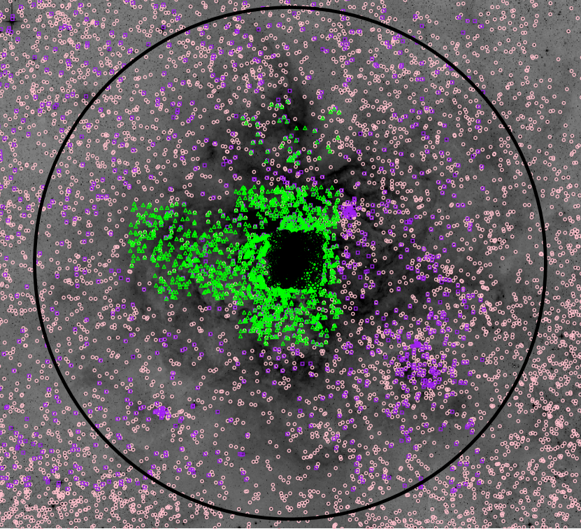
Figure 1: The spatial coverage of photometric sources from the four main catalogues used in the census, overlaid on a $V$-band WFI image. Selman (black circles), WFI (pink circles), Parker (green triangles) and CTIO (purple squares). The large black circle marks the $r_{\mathrm{d}}=10$ arcmin region of the census. North is up and East is to the left.

Due to high crowding in the central regions, space-based photometry (and spectroscopy) was favoured for stars within $r_{\mathrm{d}}<20$ arcsec (5 pc). From here onwards, when discussing the census, the term “R136 region” will refer to this $r_{\mathrm{d}}<20$ arcsec region. DeMarchi:2011 provided HST/Wide Field Camera 3 (HST/WFC3) photometry for the R136 region stars in the F336W, F438W and F555W bands. Similarly, HST/Wide Field Planetary Camera (HST/WFPC) photometry (F336W, F439W, F569W bands) from Walborn:1999 was used for stars within the dense cluster, Brey 73.

As some regions were covered by multiple catalogues, attempts were made to exclude any duplicates. Searches for sources within 0.5 arcsec of each other were made. Any that were found were subject to the same selection priority as in Paper I, based on the quality of the photometry (Selman was the primary dataset in central regions (excl. the R136 region). If the source lay beyond the Selman region, WFI was used. In the case of brighter sources, Parker was used, otherwise CTIO was used in outer regions of 30 Dor). DeMarchi:2011 was favoured for all sources in the R136 region. Table 1 gives a breakdown of the number of candidates, and spectroscopically confirmed, hot luminous stars that were selected from each photometric catalogue.

We assumed that all W-R stars in the region had been previously identified through spectroscopy (although note the recent discovery of the WN 5h star VFTS 682; Bestenlehner:2011) and while their photometry was not used for their selection (see Section 3), it would still be needed to determine stellar parameters. Issues can arise when using Johnson broad band filters with emission line stars as it can lead to a false reading of the stellar continuum and overestimate their magnitudes. A more reliable measurement is obtained through narrow band filters (Smith:1968). For all W-R stars, narrow band $b$ & $v$ magnitudes were either adopted from past work or calculated through spectrophotometry (see Appendix LABEL:sec:W-R_stars for more details).

Table 1: The literature used to select the 1145 photometric candidates and classify the 500 spectroscopically confirmed hot luminous stars in the census. The number in brackets represents those located within the R136 region. Papers which form part of the VFTS series are identified with ‘(VFTS)’.

Source of Photometry	Candidates	Confirmed (in R136)
DeMarchi:2011	212	70 (70)
Selman:1999	200	123 (2)
WFI (Paper I)	518	196 (0)
Parker:1993	71	42 (0)
CTIO (Paper I)	126	57 (0)
Walborn:1999	15	10 (0)
Zaritsky:2004	3	1 (0)
Source of Spectral Type		Confirmed (in R136)
SchildTestor:1992		7 (0)
Parker:1993		3 (0)
WalbornBlades:1997		8 (0)
MasseyHunter:1998		38 (38)
CrowtherDessart:1998		8 (8)
Bosch:1999		24 (0)
Walborn:1999		9 (0)
Breysacher:1999		3 (0)
Evans:2011 / Paper I	(VFTS)	16 (1)
Taylor:2011	(VFTS)	1 (0)
Dufton:2011	(VFTS)	1 (0)
CrowtherWalborn:2011		7 (6)
Henault-Brunet:2012a	(VFTS)	15 (14)
	(VFTS)	295 (5)
	(VFTS)	35 (0)
This work	(VFTS)	30 (0)

3 Candidate Selection

Of the tens of thousands of photometric sources included in our $r_{\mathrm{d}}<10$ arcmin spatial cut, we only seek to select the hottest and most luminous stars for the census, to estimate the stellar feedback. The hottest stars will produce the bulk of the ionising photons while the most luminous early type stars will have the strongest stellar winds, hence the largest wind luminosity. Therefore, from all the 30 Dor stars, we wish to account for all the W-R and O-type stars, along with the earliest B-type stars (given their large numbers and high $T_{\mathrm{eff}}$) and B-supergiants (given their strong winds). Various colour and magnitude cuts were applied to the photometric data to extract these stars without prior knowledge of their spectral classification.

In order to determine the boundaries of these cuts, an initial test was carried out upon the VFTS sample for which we did have a known SpT. Figure 2 shows a colour-magnitude diagram of all the VFTS O and B-type stars. The left vertical line aims to eliminate all stars with unreliable photometry, given that a typical unreddened O-type star is expected to have an observed colour of $B-V=-0.32$ mag (Fitzgerald:1970). Stars that lie to the left of this line would therefore be ‘too blue’. Similarly, the right vertical line eliminates late-type stars; too cool to contribute to the overall feedback. However, the W-R, O and early B-type stars that we do seek, can still suffer from interstellar reddening which will shift them to the lower right hand side of the diagram. The boundary was therefore set to $B-V=0.8$ mag to account for as many potentially highly reddened hot stars as possible, whilst keeping the number of unwanted, cooler stars to a minimum.

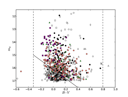
Figure 2: A colour magnitude diagram of all the VFTS O-type stars (filled) and B-type stars (open). Photometry is from: Selman (black circles), WFI (pink circles), Parker (green triangles), CTIO (purple squares). Solid and dashed lines mark the $M_{V}$ and $B-V$ colour cuts made on the sample, respectively.

In an attempt to identify the most luminous stars, a further magnitude cut was made with the diagonal reddening line. This line has a gradient which is equivalent to $R_{V}=A_{V}/E(B-V)$ (Cardelli:1989). For candidate selection, we adopt a uniform reddening value of $R_{V}=3.5$ although a value of $R_{V}=4.2$ was favoured for stars in the R136 region when determining their stellar parameters (see Appendix C for details). Individual tailored analyses for the extinction of the VFTS O-type stars are currently being carried out . Comparing these to the extinctions from our uniform $R_{V}$ value gave a mean difference of $\Delta A_{V}<0.15$ mag. We therefore continued with our approach given this relatively small offset and the likely larger uncertainties that would arise in stellar parameters, owing to the use of spectroscopic calibrations.

The magnitude cut begins at $m_{V}=15$ mag and $B-V=-0.32$ mag. This would be the position of the faintest stars we seek if they suffered from no reddening at all, corresponding to $M_{V}\approx-3.5$ mag. A star suffering from interstellar reddening, however, is expected to be shifted along the diagonal line. A value of $R_{V}=3.5$ ensured the inclusion of all the most luminous stars. While Figure 2 shows that some VFTS O-type stars are omitted (those below the line), almost all were found to be O9 or later, and given their position on the diagram, would be subluminous and hence have negligible contributions to the feedback (see Sections 8.1 & 8.2 for a quantitative discussion). Combining $R_{V}$ with our limit of $B-V=0.8$ mag allows us to account for extinctions up to $A_{V}=3.9$ mag.

A further method was also applied to select our hot luminous stars involving the ‘$Q$-parameter’ or reddening free index (Aparicio:1998). The $Q$-parameter incorporates $U$-band photometry and takes advantage of the fact that different SpTs may have similar $B-V$ colours but have different $U-B$ colours. After adjusting the relationship for 30 Dor using the reddening laws of Cardelli:1989, the $Q$-parameter took the form of $Q=(U-B)-0.67\times(B-V)$. A limit of $Q<-0.65$ was selected to filter out any mid-late B-type dwarfs and later SpT stars. This removed a further 26 stars from our candidate list and would ideally have been the best selection criterion to use. Unfortunately reliable $U$-band photometry was only available for a small subset of the sources. Furthermore, as some spurious detections had been noted in the Parker:1993 and CTIO catalogues, a further visual inspection was made of all of their sources that survived the selection cuts, to ensure that they were, indeed, true stellar sources.

An exception was made when selecting W-R and Of/WN stars. Their notably high contribution to the stellar feedback meant that all needed to be accounted for. Some W-R stars were rejected by the selection criteria mentioned, due to the unusual colours that can be brought about by their broad emission lines. For this reason, all of the W-R and Of/WN stars given in Table 2 of Paper I were manually entered into the census along with any further known W-R stars listed by Breysacher:1999 in our selected region.

A total of 1145 candidate hot luminous stars (see Table 17, Appendix D) were finally selected from the photometry via the criteria discussed above.

4 Spectroscopy

Having selected our candidate hot luminous stars, the aim was now to match as many of these as possible to spectral classifications. The best and most extensive stellar spectroscopy of 30 Dor is offered by the VFTS (Paper I). So far, all of the $\sim 360$ VFTS O-type stars have been classified including any binary companions where possible . Classification of VFTS B-type stars is currently underway. B-dwarfs and giants included in the census were classified in this work while the identified B-supergiants will become available in McEvoy et al. . Further matches were made to classifications by Bosch:1999, WalbornBlades:1997, Parker:1993 and SchildTestor:1992.

SpT matching was achieved by setting a proximity distance of $<1$ arcsec between the position of the photometric candidates and the spectral catalogues. This method relies on accurate and consistent astrometry. The SpTs of Bosch:1999 followed on from the photometric work of Selman:1999 and so checks were made to ensure authentic matching. The same was done for SpTs taken from WalbornBlades:1997 as they provided a Parker:1993 alias to the stars they classified. For any stars that did become matched with more than one SpT (most likely due to a nearby star in the field of view), the original photometry and that from the spectral catalogue were compared, with the SpT showing the most consistent photometry being selected. About 30 classified stars lacked a luminosity class. These were estimated (only for the purpose of calculating stellar parameters) by taking their derived $M_{V}$ and comparing them to the average $M_{V}$ of stars in the census of that known SpT (see Table LABEL:tab:Average_absolute_magnitudes).

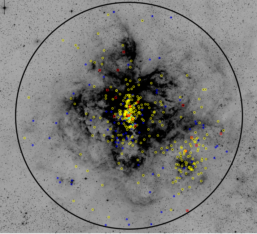
Figure 3: All the spectroscopically confirmed hot luminous stars within 30 Dor ($r_{\mathrm{d}}=10$ arcmin indicated by the large black circle), overlaid on a $V$-band WFI image. W-R stars (red squares), Of/WN stars (cyan triangles), O-type stars (yellow circles) and B-type stars (blue diamonds). North is up and East is to the left.

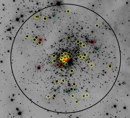
Figure 4: All the spectroscopically confirmed hot luminous stars within the R136 region ($r_{\mathrm{d}}=20$ arcsec indicated by large the black circle), overlaid on a F555W HST/WFC3 image. W-R stars (red squares), Of/WN stars (cyan triangles), O-type stars (yellow circles). North is up and East is to the left.

Within R136, stars were individually matched to the SpTs of MasseyHunter:1998, CrowtherWalborn:2011 and CrowtherDessart:1998, along with a few VFTS star classifications (Henault-Brunet:2012a). For the crowded Brey 73 cluster, we use the same SpTs obtained by Walborn:1999.

A total of 31 W-R and Of/WN stars were manually entered into the census. If they were VFTS stars, spectral classifications were taken from Table 2 of Paper I, while non-VFTS stars took their classifications from various literature: MasseyHunter:1998, Breysacher:1999 or CrowtherWalborn:2011, and references therein.

Inevitably, duplications occurred, with some stars having been classified in multiple previous studies. As with the photometry, an order of priority was assigned to the literature when selecting a SpT. If available, a VFTS classification (e.g. Paper I, Taylor:2011, Dufton:2011, Henault-Brunet:2012a, Walborn et al. , McEvoy et al. or this work) was always favoured because of the often high data quality and homogeneity of the approach. Otherwise, classifications by Bosch:1999 were adopted, followed by WalbornBlades:1997 and SchildTestor:1992 and in turn Parker:1993. Table 1 indicates the number of stars classified from each reference. Note that a larger number of stars were matched to spectra as indicated in Table 2. Table 1 only lists the spectroscopically confirmed hot luminous stars for which stellar parameters and feedback were later determined. Figure 3 gives the spatial distribution of the classified stars listed in Table 1. Figure 4 provides a closer look at the central crowded R136 region.

5 Spectroscopic Completeness

In this section we aim to estimate the spectroscopic completeness of hot luminous stars in 30 Dor. Figure 5 presents a set of colour magnitude diagrams, similar to that in Figure 2, now including all photometrically selected stars in the census. Approximately 60% of stars in the census have available spectroscopy, either from the VFTS or a previous study. The different SpTs of these stars are shown and also listed in Table 2.

Overall, 40% of candidates lacked spectroscopy. However, this fraction rises as one moves to increasingly redder and fainter stars. This is expected since obtaining high quality spectroscopy for fainter stars is much more difficult. As explained in Section 3, more contaminant (later than B-type) stars will be found in the lower right hand side of Figure 5. Ideally, these contaminants would have been removed through the $Q$-parameter cut but the limited availability of $U$-band photometry meant this was rarely possible. The key question is what fraction of the unclassified stars are in fact hot luminous stars, and what would the spectroscopic completeness be if they were taken into account? Figure 5 shows that the stars with spectroscopy are governed by the magnitude limit of the VFTS ($m_{V}<17$ mag). Therefore, an accurate spectroscopic completeness level can only really be estimated for stars brighter than this limit.

Table 2: The spectral type distribution of all the stars meeting the photometric selection criteria in Section 3.

ALL STARS	1145
Stars without spectra	463
Stars with spectra	VFTS (% of Total)	non-VFTS	Total
W-R	17 (68)	8	25
Of/WN	6 (100)	0	6
O-type	322 (84)	63	385
B-type	219 (92)	18	237
later than B-type	21 (72)	8	29
Total	585 (86)	97	682

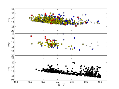
Figure 5: Colour magnitude diagrams of all the stars meeting the selection criteria. Stars with VFTS spectral classification (top), stars with non-VFTS spectral classification (middle) and stars with no spectral classification (bottom). Key for classified stars: W-R stars (red squares), Of/WN stars (cyan triangles), O-type stars (yellow circles), B-type stars (blue diamonds) and stars later than B-type (crosses).

From this point onwards, we define a separate region, the ‘MEDUSA region’ ($0.33<r_{\mathrm{d}}<10$ arcmin) along with our previously defined ‘R136 region’ ($r_{\mathrm{d}}<20$ arcsec). Using a distance modulus of 18.49 mag these regions span projected radii of about $5<r_{\mathrm{d}}<150$ pc and $r_{\mathrm{d}}<5$ pc, respectively. This allowed for a less biased measure of the spectroscopic completeness of the VFTS since its FLAMES/MEDUSA observations (see Paper I) largely avoided the R136 vicinity because of crowdedness.

5.1 Spectroscopic completeness in the MEDUSA region

Figures 6 & 7 show histograms of the number of photometric candidates for which spectroscopy was available, in relation to magnitude and colour, respectively. Within the MEDUSA region, 80% of candidates have been spectroscopically observed of which about three quarters were included in the VFTS. Of these, only a subset were spectroscopically confirmed as hot luminous stars. These are the stars given in Table 3.

Figure 6: The spectroscopic completeness, with respect to $m_{V}$, of all stars in the MEDUSA region meeting the selection criteria and with $m_{V}<17$ mag. Stars with VFTS spectroscopy (red), stars with non-VFTS spectroscopy (cyan) and stars with no spectroscopy (black).

In an attempt to obtain an accurate completeness level for the region, Figure 8 gives the fraction of stars that are spectroscopically confirmed as hot luminous stars as a function of colour. Moving redward of the typical O-type star intrinsic colour $(B-V)_{\mathrm{o}}=-0.32$ mag, the fraction is seen to fall from unity as more contaminants populate each colour bin. At high values of $B-V$, these fractions become poorly constrained as a result of small number statistics. By accounting for the fraction of contaminants, a new completeness plot can be made as shown in Figure 9 which, unlike Figure 7, has had the predicted contaminant stars removed. Applying this correction, the completeness of the hot luminous stars is estimated at 84%, of which 76% were included in the VFTS.

Table 3: The spectral type distribution of the spectroscopically confirmed hot luminous stars within the MEDUSA region ($5<r_{\mathrm{d}}<150$ pc).

W-R and Of/WN stars	WR2-WR5		WR6-WR9		Total
WN or WN/C	7		8		15
WC	3		0		3
Of/WN	0		1		1
Total	10		9		19
O-type stars	O2-3.5	O4-6.5		O7-9.7	Total
V	15	60		143	218
III	5	11		66	82
I	2	3		20	25
Total	22	74		229	325
B-type stars	B0-0.7		B1 and later		Total
V	24		-		24
III	15		7		22
I	12		26		38
Total	51		33		84
GRAND TOTAL					428

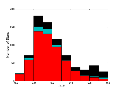
Figure 7: The spectroscopic completeness, with respect to $B-V$, of all stars in the MEDUSA region meeting the selection criteria and with $m_{V}<17$ mag. Colours are as in Figure 6.

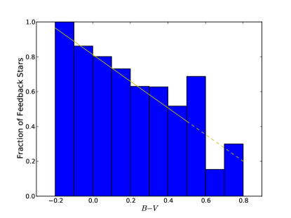
Figure 8: The fraction of stars in the MEDUSA region meeting the selection criteria and with both $m_{V}<17$ mag and spectra, which were spectroscopically confirmed to be hot luminous stars. A low order polynomial was fitted to the distribution (solid line) and extrapolated redward of $B-V=0.5$ mag (dashed line).

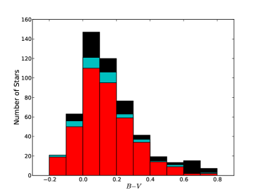
Figure 9: The spectroscopic completeness of hot luminous stars with $m_{V}<17$ mag in the MEDUSA region, with respect to $B-V$. Colours are as in Figure 6.

5.2 Spectroscopic completeness in the R136 region

Figure 10 shows that only the brightest targets ($\approx 35$%) in the R136 region have archival spectroscopy, primarily obtained with HST/FOS by MasseyHunter:1998, with the VFTS covering only a limited number of stars through its FLAMES-ARGUS observations (see Paper I and Henault-Brunet:2012a). A breakdown of their SpTs is listed in Table 4. This will be improved following new HST/STIS spectroscopy of the central parsec (GO 12465/13052, P.I. - P. Crowther). Figure 11 suggests that these unclassified stars are predominantly early type stars i.e. mid-late O-type stars which eluded spectroscopic confirmation, simply because they are faint. More importantly, completeness is still high at the brighter end, and includes the more luminous W-R, Of/WN and supergiant stars which will contribute most to the feedback of the region. We therefore estimate that 35% of the hot luminous stars have so far been spectroscopically observed.

Table 4: The spectral type distribution of the spectroscopically confirmed hot luminous stars within the R136 region ($r_{\mathrm{d}}<5$ pc).

W-R and Of/WN stars	WR2-WR5		WR6-WR9		Total
WN or WN/C	5		1		6
WC	1		0		1
Of/WN	3		2		5
Total	9		3		12
O-type stars	O2-3.5	O4-6.5		O7-9.7	Total
V	19	11		11	41
III	9	0		2	11
I	4	4		0	8
Total	32	15		13	60
GRAND TOTAL					72

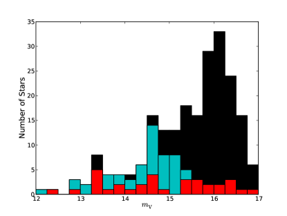
Figure 10: The same as Figure 6, only showing completeness in the R136 region. Colours are as in Figure 6.

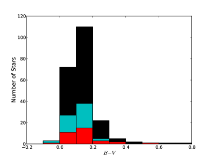
Figure 11: The same as Figure 7, only showing completeness in the R136 region. Colours are as in Figure 6.

5.3 Stars unaccounted for

While we attempt to include all the potential hot luminous stars in 30 Dor, the following factors may have prevented certain candidates from entering our final census:

1. Crowding - Our four primary photometry catalogues (Selman, WFI, Parker, CTIO) provided sound coverage of 30 Dor. Potential concern arises in dense regions where candidates may have been lost as a result of less reliable photometry.

2. High extinction - We calculate an average extinction of $A_{V}\approx 1.5$ mag for 30 Dor, with our selection criteria allowing for extinctions as high as $A_{V}=3.92$ mag. For some stars, the extinction will be higher than this limit. In particular, young embedded stars will have evaded selection through their surrounding gas and dust but could still contribute to the stellar feedback (see Section 8.3).

3. Spectroscopic Completeness - Section 5 showed a good spectrosopic completeness for the census but the remaining stars lacking spectroscopy are still important and their contribution is considered in Section 5.4. Furthermore, the magnitude coverage of the spectroscopy was limited to $m_{V}<17$ mag. This means that a few faint and highly reddened hot luminous stars could also have avoided classification.

4. Binary systems - Stars found in binary systems will provide further candidates through their companions as well as changing the photometric properties of each component. Section 6.5 addresses the case of double-lined (SB2) binary systems where a knowledge of both stars can provide a combined feedback contribution but single-lined (SB1) binary systems and any further unknown multiple systems, remain uncertain.

5. Unresolved stellar systems - Spectroscopic binary detection is limited to shorter periods of a few days. While HST imaging is capable of revealing likely composite spectra, many large separation and/or line of sight systems will still appear single and are so far unidentified.

5.4 Correcting for unclassified stars

Section 5.1 looked at removing the estimated number of contaminant stars in different colour bins. Even after applying this method to determine the true number of hot luminous stars, some still lack spectroscopy. For the MEDUSA region, a total of 152 of our candidates ($m_{V}<17$ mag) lacked spectroscopy, of which it was estimated that only $\approx 50$% would actually be hot luminous stars. Meanwhile, in R136, 141 candidates ($m_{V}<17$ mag) lacked spectroscopy but in this case, all were taken to be hot luminous stars capable of contributing to the feedback. This is a reasonable assumption given that all other R136 stars in the census are classified as W-R, Of/WN or O-type stars. Furthermore, as noted earlier, the magnitudes and colours of these unclassified stars suggest them to be mid-late O-type stars.

Voges:2008 estimated the SpT of unclassified stars in their LMC H ii regions using a colour-SpT calibration. It was based on $U$- and $B$-band magnitudes as these lay closest to the peaks in the spectral distributions of the OB stars. However, this approach relied upon accurate photometry, and in the case of the $U$-band, this was only available for a select number of our stars. The $M_{V}$ was therefore calculated for each star, assuming a common intrinsic colour of $(B-V)_{\mathrm{o}}=-0.3$ mag. Its SpT was then estimated based on this $M_{V}$, using the average $M_{V}$ found for each SpT in the rest of the census (see Table LABEL:tab:Average_absolute_magnitudes). Some crude assumptions had to be made when more than one luminosity class was consistent with the $M_{V}$. In R136, stars were typically assumed to be dwarfs given the young age of the region. All W-R and Of/WN stars were assumed to be already accounted for.

6 Stellar Calibrations

With photometry and a SpT assigned to as many stars as possible, the aim was now to estimate their feedback. Here we specifically seek the radiative and mechanical stellar feedback. We determined the radius independent Lyman continuum ionising flux per cm^-2 ($q_{\mathrm{0}}$). This is related to the total number of ionising photons emitted by the star per second ($Q_{\mathrm{0}}$) via $Q_{\mathrm{0}}=4\pi R^{2}q_{\mathrm{0}}$, where $R$ is the stellar radius at a Rosseland optical depth of two thirds ($R_{2/3}$), or in the case of W-R stars, the radius at an optical depth of $\sim 10$ ($R_{*}$). Similarly, if we omit the effects of supernovae, our primary source of mechanical feedback is that produced by the stellar winds. The stellar wind luminosity ($L_{\mathrm{SW}}$) is calculated via $L_{\mathrm{SW}}=\frac{1}{2}\dot{M}\varv_{\infty}^{2}$, where $\dot{M}$ is the mass-loss rate of the star, $\varv_{\infty}$ is the terminal velocity of the stellar wind and $L_{\mathrm{SW}}$ is given in units of erg s^-1. In addition, we also calculated the modified wind momentum $D_{\mathrm{mom}}=\dot{M}\varv_{\infty}R^{0.5}$.

Detailed atmospheric analyses are currently underway of all the VFTS stars which will eventually be used to assign each stellar parameter. In this study, however, we turn to a variety of calibrations to supply the parameters. Results for W-R and Of/WN stars were based on atmospheric models, given their important role in feedback contribution.

6.1 O-type stars

A total of 385 O-type stars were selected within 30 Dor. The calibrations for the O-type star parameters were based primarily on the models of Martins:2005. Their $T_{\mathrm{eff}}$-SpT scale was revised by $+1$ kK for the LMC environment (Mokiem:2007; RiveroGonzalez:2012a) while the earliest subtypes (O2-O3.5) had $T_{\mathrm{eff}}$ individually selected, based on the works of RiveroGonzalez:2012b and DoranCrowther:2011. New calibrations for the bolometric correction ($BC$) and $q_{\mathrm{0}}$ were also derived. Tables 5-7 provide a summary of the O-type star parameters used. Further empirical and theoretical data helped to obtain the stellar wind parameters. Values of $\varv_{\infty}$ were sourced from Prinja:1990 while mass-loss rates were predicted using the theoretical prescriptions of Vink:2001. See Appendix LABEL:sec:O-star_Calibrations for more details.

Table 5: O-type star parameters for luminosity class V.

SpT	$T_{\mathrm{eff}}$	$BC_{V}$	log $q_{\mathrm{0}}$	$L_{\mathrm{EUV}}$	$\varv_{\infty}$
	(kK)	(mag)	(ph cm-2 s-1)	($L_{\mathrm{Bol}}$)	(km s-1)
O2	54.0	$-4.61$	24.97	0.74	3300
O3	48.0	$-4.26$	24.70	0.61	3000
O3.5	47.0	$-4.19$	24.65	0.58	3300
O4	43.9	$-3.99$	24.52	0.50	3000
O5	41.9	$-3.84$	24.41	0.44	2700
O5.5	40.9	$-3.77$	24.34	0.42	2000
O6	39.9	$-3.70$	24.27	0.39	2600
O6.5	38.9	$-3.62$	24.20	0.36	2500
O7	37.9	$-3.55$	24.11	0.32	2300
O7.5	36.9	$-3.47$	24.01	0.29	2000
O8	35.9	$-3.39$	23.90	0.26	1800
O8.5	34.9	$-3.31$	23.78	0.23	2000
O9	33.9	$-3.22$	23.64	0.19	1500
O9.5	32.9	$-3.14$	23.49	0.16	1500
O9.7	32.5	$-3.11$	23.43	0.14	1200

Table 6: O-type star parameters for luminosity class III.

SpT	$T_{\mathrm{eff}}$	$BC_{V}$	log $q_{\mathrm{0}}$	$L_{\mathrm{EUV}}$	$\varv_{\infty}$
	(kK)	(mag)	(ph cm-2 s-1)	($L_{\mathrm{Bol}}$)	(km s-1)
O2	49.6	$-4.34$	24.78	0.65	3200
O3	47.0	$-4.20$	24.67	0.58	3200
O3.5	44.0	$-4.01$	24.54	0.50	2600
O4	42.4	$-3.90$	24.46	0.46	2600
O5	40.3	$-3.75$	24.34	0.40	2800
O5.5	39.2	$-3.67$	24.27	0.37	2700
O6	38.2	$-3.58$	24.20	0.33	2600
O6.5	37.1	$-3.50$	24.12	0.30	2600
O7	36.1	$-3.41$	24.03	0.27	2600
O7.5	35.0	$-3.32$	23.93	0.23	2200
O8	34.0	$-3.23$	23.82	0.20	2100
O8.5	32.9	$-3.13$	23.70	0.16	2300
O9	31.8	$-3.03$	23.58	0.12	1900
O9.5	30.8	$-2.93$	23.44	0.08	1500
O9.7	30.4	$-2.89$	23.38	0.07	1200

Table 7: O-type star parameters for luminosity class I.

SpT	$T_{\mathrm{eff}}$	$BC_{V}$	log $q_{\mathrm{0}}$	$L_{\mathrm{EUV}}$	$\varv_{\infty}$
	(kK)	(mag)	(ph cm-2 s-1)	($L_{\mathrm{Bol}}$)	(km s-1)
O2	46.0	$-4.10$	24.63	0.60	3000
O3	42.0	$-3.88$	24.45	0.52	3700
O3.5	41.1	$-3.81$	24.40	0.50	2000
O4	40.1	$-3.75$	24.35	0.48	2300
O5	38.3	$-3.61$	24.23	0.43	1900
O5.5	37.3	$-3.53$	24.17	0.40	1900
O6	36.4	$-3.45$	24.10	0.38	2300
O6.5	35.4	$-3.37$	24.03	0.35	2200
O7	34.5	$-3.28$	23.95	0.32	2100
O7.5	33.6	$-3.20$	23.86	0.29	2000
O8	32.6	$-3.10$	23.77	0.25	1500
O8.5	31.7	$-3.01$	23.67	0.22	2000
O9	30.7	$-2.91$	23.56	0.18	2000
O9.5	29.8	$-2.81$	23.45	0.15	1800
O9.7	29.4	$-2.77$	23.40	0.13	1800

6.2 B-type stars

A total of 84 B-type stars were selected within 30 Dor. Most B-type star parameters were estimated using existing calibrations. $T_{\mathrm{eff}}$ was adopted from Trundle:2007 and $BC_{V}$ calculated from the relations of Crowther:2006 for supergiants, or LanzHubeny:2003 in the case of dwarfs and giants. A new calibration was derived for $q_{\mathrm{0}}$ based on the work of Smith:2002, Conti:2008 and RiveroGonzalez:2012a. Table 8 gives a summary of the B-type star parameters used. Prinja:1990 once again supplied $\varv_{\infty}$, along with KudritzkiPuls:2000. In the case of early B-dwarfs and giants, where no known $\varv_{\infty}$ are published, we assume a value of $\varv_{\infty}=1000$ km s^-1 given that wind properties are expected to be similar to their late O-type star counterparts.

We again employ the Vink:2001 prescription for B-dwarfs and giants but opted not to use it for B-supergiants following discrepancies with empirical results noted by (MarkovaPuls:2008; TrundleLennon:2005). Instead we turned to using the wind-luminosity relation (WLR, Kudritzki:1999), whereby the modified wind momentum ($D_{\mathrm{mom}}=\dot{M}\varv_{\infty}R^{0.5})$ is shown to relate to the stellar luminosity. See Appendix LABEL:sec:B-star_Calibrations for more details.

Table 8: B-type star parameters for all luminosity classes.

SpT	$T_{\mathrm{eff}}$	$BC_{V}$	$\log q_{\mathrm{0}}$	$L_{\mathrm{EUV}}$	$\varv_{\infty}$
	(kK)	(mag)	(ph cm-2 s-1)	($L_{\mathrm{Bol}}$)	(km s-1)
Luminosity Class V
B0	31.4	$-3.04$	23.15	0.11	1000
B0.2	30.3	$-2.93$	22.85	0.06	1000
B0.5	29.1	$-2.81$	22.56	0.02	1000
Luminosity Class III
B0	29.1	$-2.81$	22.56	0.02	1000
B0.2	27.9	$-2.68$	22.28	$<0.01$	1000
B0.5	26.7	$-2.55$	22.02	$<0.01$	1000
B0.7	25.4	$-2.41$	21.78	$<0.01$	1000
B1	24.2	$-2.26$	21.56	$<0.01$	1000
Luminosity Class I
B0	28.6	$-2.71$	22.86	0.10	1500
B0.2	27.0	$-2.58$	22.51	0.03	1400
B0.5	25.4	$-2.44$	22.17	0.03	1400
B0.7	23.8	$-2.30$	21.84	0.01	1200
B1	22.2	$-2.14$	21.52	$<0.01$	1100
B1.5	20.6	$-1.97$	21.22	$<0.01$	800
B2	19.0	$-1.79$	20.93	$<0.01$	800
B2.5	17.4	$-1.60$	20.65	$<0.01$	800
B3	15.8	$-1.38$	20.39	$<0.01$	600
B5	14.2	$-1.14$	20.13	$<0.01$	500
B8	12.3	$-0.83$	19.86	$<0.01$	200

6.3 Uncertainties in calibrations

All of the stellar calibrations are open to various uncertainties. Most important to estimating an accurate ionising luminosity will be our adopted $T_{\mathrm{eff}}$-SpT calibration. Martins:2005 and Trundle:2007 would suggest uncertainties on $T_{\mathrm{eff}}$ of about $\pm 1-2$ kK, likely to be higher ($\pm 3-4$ kK) in the case of our earliest O-type stars.

The $BC_{V}$ of the stars are particularly dependent on $T_{\mathrm{eff}}$ (Martins:2005; MartinsPlez:2006). Given the low extinction of 30 Dor and renewed accuracy in its distance (Pietrzynski:2013), it is the $BC_{V}$ of the stars which dominates the uncertainty of their bolometric luminosity ($L_{\mathrm{Bol}}$). The uncertainty on $\log L_{\mathrm{Bol}}/{\mathrm{L}}_{\odot}$ is found to be about $\pm 0.15-0.25$ dex. With $T_{\mathrm{eff}}$ similarly affecting the values of $q_{\mathrm{0}}$, our final ionising luminosities, $Q_{\mathrm{0}}$, are expected to be accurate to within $\sim 60$%.

A reliable wind luminosity depends on the accuracy of $\dot{M}$ and $\varv_{\infty}$. The assignment of $\varv_{\infty}$ was primarily based on the observational UV study by Prinja:1990. It remains one of the most extensive works yet many SpTs rely on only a couple of measurements. Again, these were carried out on Galactic OB stars, but a metallicity dependence is noted for $\varv_{\infty}$ (Leitherer:1992 derive $\varv_{\infty}\propto Z^{0.13}$). Given the limited data for some SpT we do not attempt to correct for this dependence. However, in the case of the earliest stars (O2-3.5), values were supplemented by the later work of PrinjaCrowther:1998, Massey:2004 and DoranCrowther:2011, who studied further O-type stars, this time in the Magellanic Clouds.

In the case of our mass-loss rates, wind clumping is not directly accounted for in the Vink:2001 prescription. The effects of clumping have been thought to potentially scale down $\dot{M}$ by a factor of a few. However, Mokiem:2007b argued that if a modest clumping correction is applied to empirical mass-loss rates, a better consistency is found with the Vink:2001 prescription.

The uncertainties on our adopted SpT ($\approx\pm 0.5$) should be insignificant when compared to those of our stellar parameters. Any SpT will naturally show a spread in parameters, however, over the entire census, such uncertainties are expected to balance out to provide first order estimates of the feedback. To test this, the properties of a selection of O2-3 type stars in 30 Dor which had been previously modelled (RiveroGonzalez:2012b; Evans:2010; Massey:2005), were compared to those of our calibrations. Offsets up to a factor of 2 were found but typically our estimates of $Q_{\mathrm{0}}$, $L_{\mathrm{SW}}$ and $D_{\mathrm{mom}}$ were within $\sim 40$% of values obtained from tailored analyses.

6.4 Wolf-Rayet and Of/WN stars

A total of 25 W-R and 6 Of/WN stars are located within our census region. The significance of such stars to the integrated properties of young star clusters was demonstrated by CrowtherDessart:1998, who estimated a contribution of 15% and 40% to the ionising and wind luminosities, respectively, out to a radius of 10 pc from R136a1. However, their results were based upon non-line blanketed W-R models and historical OB star calibrations.

In view of the importance of W-R stars to our census of 30 Dor, we took the following approach. We analysed a single example of each W-R and Of/WN subtype using the non-local thermodynamic equilibrium (non-LTE) atmospheric code CMFGEN (HillierMiller:1998), which was used as a template for other stars. CMFGEN solves the radiative transfer equation in the co-moving frame, subject to radiative and statistical equilibrium. Since CMFGEN does not solve the momentum equation, a density/velocity structure is required. For the supersonic part, an exponent of $\beta=1$ is adopted for the velocity law, while the subsonic velocity structure is defined using a plane-parallel TLUSTY model (LanzHubeny:2003).

Stellar temperatures, $T_{*}$, correspond to a radius at Rosseland optical depth of 10, and are consequently somewhat higher than effective temperatures, $T_{\mathrm{eff}}$, relating to an optical depth of two thirds. Wind clumping is incorporated using a radially dependent volume filling factor, $f$, with $f_{\infty}=0.1$ at $\varv_{\infty}$, resulting in a reduction in mass-loss rate by a factor of $f^{-0.5}\sim 3$ with respect to a smooth wind.

CMFGEN incorporates line blanketing through a super level approximation, in which atomic levels of similar energy are grouped into a single super level that is used to compute the atmospheric structure. For WN and Of/WN subtypes, the model atoms include H i, He i-ii, C iii-iv, N iii-v, O iii-vi, Si iv, P iv-v, S iv-vi and Fe iv-vii while WC model atoms comprise He i-ii, C ii- iv, O ii-vi, Ne ii-vi, Si iv, P iv-v, S iv-vi, Ar iii-viii and Fe iv-viii. Other than H, He, CNO, we adopt half-solar abundances (Asplund:2009).

In some instances, previous CMFGEN tailored analyses of individual stars have been undertaken, which are not repeated here. Crowther:2010 have studied the bright WN stars within R136, whose properties are adopted here, while we use R136a3 (BAT99-106) as a template for other WN 5 stars. In addition, Crowther:2002 undertook a tailored analysis of the WC 4 star BAT99-90 (Brey 74), which also serves as a template for other WC stars.

For the remaining template stars, observational datasets are taken from a variety of sources, including IUE, HST (far-ultraviolet spectrophotometry), AAT/RGO, SSO 2.3m/DBS, MSO 1.9m/Coude (optical spectrophotometry) and VLT/UVES, VLT/FLAMES (optical spectroscopy). Inevitably, the stars used as templates suffer from our reliance upon heterogeneous spectroscopic and photometric datasets. Inferred physical and wind properties for these template emission line stars are presented in the Appendix (Table LABEL:tab:W-R_and_Of/WN_star_parameters), together with spectroscopic fits (Figures LABEL:fig:plot_sk6722-LABEL:fig:plot_bat90). Narrow-band magnitudes are used in preference to broad-band magnitudes, where available, owing to the non-zero effects of emission lines on the latter. Interstellar extinctions are calculated for an assumed $R_{V}=4.2$ (R136 region) or 3.5 (elsewhere), with the exception of Sk-67^∘ 22 (O2 If*/WN5, CrowtherWalborn:2011) for which $R_{V}=3.1$ is adopted. Bestenlehner et al. have undertaken a study of luminous O, Of/WN and WN stars from the VFTS which should be preferred to results from the present study, owing to the use of homogeneous datasets and an extensive grid of CMFGEN models.

For non-template stars, stellar temperatures and wind densities were adopted from the relevant template, with other parameters (mass-loss rates, luminosities) scaled to their respective absolute (narrow-band) magnitudes. In cases where a W-R star was known to be multiple, such as R132 and R140, absolute magnitudes for the W-R component(s) were obtained from the dilution in line equivalent widths with respect to single stars, as illustrated in the Appendix (Table LABEL:tab:W-R_photometry). If possible, individual $\varv_{\infty}$ were obtained from literature values (e.g. CrowtherSmith:1997), or otherwise adopted from the template star. Mass-loss rates were estimated by adopting identical wind densities (i.e. identical transformed radii, Schmutz:1989) to the template stars.

Regarding the reliability of our method, we have compared the parameters inferred for the WN 5h star VFTS 682 to those from a detailed analysis by Bestenlehner:2011 and obtain an ionising luminosity that is 50% lower than the detailed study, with a wind luminosity $\sim 60$% lower. Further comparisons await the results from Bestenlehner et al. (in prep.) for other VFTS stars in common.

Finally, following the completion of this study, in which R144 (Brey 89, BAT99-118) was selected as the template WN 6 star, Sana:2013b have revealed this to be a WN 5-6+WN 6-7 binary system. We are able to estimate the revised parameters for this system using bolometric corrections from our template WN 5+WN 7 stars. According to Sana:2013b, the mass ratio of the WN 7 secondary to WN 5 primary is $\sim 1.17$, so for an adopted $L_{\mathrm{Bol}}\propto\mathrm{M}^{1.5}$ for very massive stars (Yusof:2013), the approximate ratio of their luminosities is $1.17^{1.5}=1.26$. Based on the systemic absolute magnitude of R144 in Table LABEL:tab:W-R_photometry, the inferred absolute magnitudes of the WN 5 primary and WN 7 secondary are $-6.4$ and $-7.4$ mag, respectively, from which bolometric luminosities of $10^{6.2}$ and $10^{6.3}\,\mathrm{L}_{\odot}$ are obtained. Consequently, the systemic bolometric luminosity of R144 may be up to $10^{6.6}\,\mathrm{L}_{\odot}$, i.e. 0.2 dex higher than that obtained in Table LABEL:tab:W-R_and_Of/WN_star_parameters.

6.5 Binary systems

The spectroscopic binary fraction of O-type stars in 30 Dor has been estimated to be $0.51\pm 0.04$ (Sana:2013a), a considerable number of the stars in our census. In the case of these close binary systems, our photometric data will represent the combined light of both components giving an absolute magnitude for the system, $M_{V}^{\mathrm{sys}}$. For now, we have only attempted to correct for a subset of the SB2 systems, where a robust subtype and luminosity class was known for both components. This included 27 of the 48 SB2 systems identified in the census. Average absolute magnitudes from the census (Table LABEL:tab:Average_absolute_magnitudes) allowed $\Delta M_{V}=M_{V}^{1}-M_{V}^{2}$ to be estimated. Absolute magnitudes for each component (Table LABEL:tab:SB2) were then calculated from $\Delta M_{V}$ and $M_{V}^{\mathrm{sys}}$. Separate stellar parameters were also calculated for each star following the usual calibrations. SB1 and SB2 systems where complete classification of the secondary component was unavailable, were not corrected i.e. all light is assumed to have originated from the primary component.

Correcting W-R stars in multiple systems was even more important, given their feedback contributions. Details of the steps taken are set out in Appendix LABEL:sec:W-R_Binaries.

The final stellar parameters derived for all the hot luminous stars with spectroscopy are listed in Table 18.

7 Stellar Census

On the basis of our inferred stellar parameters, estimates of age and mass could be made. Figure 12 presents an H-R diagram of all the hot luminous stars in the MEDUSA region. As discussed in Section 6.3 uncertainties on $T_{\mathrm{eff}}$ are likely to be about $\pm 2000$ K while $\log L_{\mathrm{Bol}}/\mathrm{L}_{\odot}$ is accurate to $\pm 0.2$ dex. The zero-age main sequence (ZAMS) positions are based on the contemporary evolutionary models of Brott:2011 and Köhler et al. . The accompanying isochrones are overlaid for rotating ($\varv_{\mathrm{rot}}=300\,\mathrm{km\,s}^{-1}$) and non-rotating models, spanning ages from 0 to 8 Myr. The hot stars to the far left of the diagram are the evolved W-R stars. They are not covered by the isochrones as the associated evolutionary tracks only modelled as far as the terminal-age main sequence. However, the isochrones do still reveal a large age spread across more than 8 Myr. Indeed, WalbornBlades:1997 found several distinct stellar regions of different ages within 30 Dor, showing a possibility for triggered star formation.

Identifying individual age groups isn’t possible in more distant star forming regions but we attempt it for the massive R136 cluster. Figure 12 shows a similar H-R diagram for the R136 region. Its stars are typically more massive, showing a younger age, separate from the rest of 30 Dor. The isochrones suggest the most massive stars to be $\sim 1-2$ Myr old, with an older age being favoured further down the main sequence. This is largely consistent with the work of MasseyHunter:1998 who found ages $\sim 2$ Myr. Sabbi:2012 determined a similar 1-2 Myr age for R136 but also identified an older ($\sim 2-5$ Myr) region extending $\sim 5.4$ pc to the north-east. As our R136 region extends to 5 pc, there is a high possibility of contamination from older non-coeval stars.

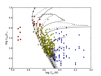
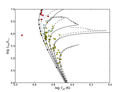
Figure 12: An H-R diagram of all the spectroscopically confirmed hot luminous stars in the MEDUSA region (a) and R136 region (b). W-R stars (red squares), Of/WN stars (cyan triangles), O-type stars (yellow circles) and B-type stars (blue diamonds). Isochrones at 1, 2, 3, & 5 Myrs are overlaid in both cases, with 8 Myr also used for the MEDUSA region. The isochrones are based on rotating ($\varv_{\mathrm{rot}}=300\,\mathrm{km\,s}^{-1}$, dashed line) and non-rotating ($\varv_{\mathrm{rot}}=0\,\mathrm{km\,s}^{-1}$, solid line) evolutionary models of Brott:2011 and Köhler et al. . The ZAMS positions for stars with $M_{\mathrm{init}}$ = 20, 40, 60, 80, 100, 120, 150, 200, 300 & 400 M_⊙ are marked by black stars and joined with a solid line.

To estimate stellar masses we applied a mass-luminosity relation of $L_{\mathrm{Bol}}\propto M^{1.75}$ for all O-type dwarfs (Yusof:2013). However, this relation strictly only applies to ZAMS stars within a mass range of $\sim 60-150$ M_⊙ and as a result would underestimate the masses for lower luminosity dwarfs. In the case of the O-type giants and supergiants, we adopted the $\log\,g$-SpT calibrations of Martins:2005. A mass was then calculated using the stellar radius produced from the parameters of our own calibrations. A similar approach was used for the B-type stars, only average $\log\,g$ values were taken for each SpT from the works of Trundle:2007 and Hunter:2007. Rough mass estimates of the WC and WN/C stars were obtained through the calibration of SchaererMaeder:1992 but in case of the hydrogen burning WN and Of/WN stars, we returned to the H-burning mass-luminosity relation.

Our photometry indicates a further 141 hot luminous stars within the R136 region and 222 stars within 30 Dor (Section 5.4). We therefore account for these stars as well when deriving the mass function for each region. In this case, the SpTs for the census were obtained through a combination of spectroscopy and photometry (Sp+Ph), as opposed to relying solely on stars that were spectroscopically classified (Sp). Our inferred mass functions for 30 Dor and the R136 region are plotted in Figure 13. There is consistency with the Salpeter:1955 $\alpha=-2.3$ slope but this notably deviates at $\sim 20$ M_⊙, due to incomplete photometry and spectroscopy. Assuming the Sp+Ph stellar census to be complete above 20 M_⊙ and adopting a Kroupa:2001 initial mass function (IMF), the total stellar mass for each region was obtained: $M_{\mathrm{30Dor}}\sim 1.1\times 10^{5}$ M_⊙ and $M_{\mathrm{R136}}\sim 5.0\times 10^{4}$ M_⊙, the latter being within $\sim 10$% of the R136 mass estimated by Hunter:1995 when a similar Kroupa IMF is adopted.

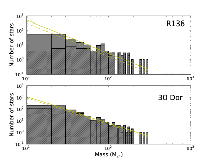
Figure 13: The present day mass function of all hot luminous stars classified spectroscopically and photometrically (Sp+Ph) in the R136 region (top) and in 30 Dor (bottom). Hatched regions indicate where the mass function is based solely on stars classified spectroscopically (Sp). A Salpeter $\alpha=-2.3$ slope is overlaid with a yellow line (solid = Sp+Ph, dashed = Sp), for which the integrated mass ($>20$ M_⊙) is consistent with that of each region.

8 Integrated Stellar Feedback

For an estimate of the total stellar feedback of 30 Dor, the contributions of individual stars were combined to produce the cumulative plots presented in Figures 14 - 15. While the R136 region showed a lower completeness compared to 30 Dor, it still contained a high proportion of the brightest W-R, Of/WN and O-type stars, and is therefore considered separately. In addition, feedback estimates are also made for the stars lacking spectroscopy (Section 5.4). The integrated feedback at different projected radial distances can be found in Table 9 along with a breakdown of the contributions from the different SpTs.

Table 9: The cumulative properties of hot luminous stars in 30 Dor with increasing projected radius, $r_{\mathrm{d}}$, given in (pc), from R136a1. The top half of the table gives the more robust values, based solely on the number of stars (N) classified spectroscopically (Sp). The bottom half combines both spectroscopically and photometrically classified stars (Sp+Ph). Note the contribution from the W-R and Of/WN stars remains unchanged as none of these stars were taken to lack spectroscopy. $\log L_{\mathrm{Bol}}$ is given in $(\mathrm{L}_{\odot})$, $Q_{\mathrm{0}}$ in $(\times 10^{49}\,\mathrm{ph}\,\mathrm{s}^{-1})$, $L_{\mathrm{SW}}$ in $(\times 10^{37}\,\mathrm{erg}\,\mathrm{s}^{-1})$ and $D_{\mathrm{mom}}$ in $(\times 10^{36}\,\mathrm{cgs\,units})$.

Region	OB Stars					W-R and Of/WN Stars					Grand Total
$<r_{\mathrm{d}}$	N	$\log L_{\mathrm{Bol}}^{\mathrm{Sp}}$	$Q_{\mathrm{0}}^{\mathrm{Sp}}$	$L_{\mathrm{SW}}^{\mathrm{Sp}}$	$D_{\mathrm{mom}}^{\mathrm{Sp}}$	N	$\log L_{\mathrm{Bol}}^{\mathrm{Sp}}$	$Q_{\mathrm{0}}^{\mathrm{Sp}}$	$L_{\mathrm{SW}}^{\mathrm{Sp}}$	$D_{\mathrm{mom}}^{\mathrm{Sp}}$	N	$\log L_{\mathrm{Bol}}^{\mathrm{Sp}}$	$Q_{\mathrm{0}}^{\mathrm{Sp}}$	$L_{\mathrm{SW}}^{\mathrm{Sp}}$	$D_{\mathrm{mom}}^{\mathrm{Sp}}$
5	60	7.61	242	37.6	2.72	12	7.66	334	63.9	7.69	72	7.93	576	101	10.4
10	120	7.77	319	48.6	3.86	13	7.67	343	65.8	8.03	133	8.02	662	114	11.9
20	191	7.88	397	59.0	4.83	19	7.74	398	85.3	9.98	210	8.12	795	144	14.8
150	469	8.07	554	75.6	6.22	31	7.84	503	122	13.7	500	8.27	1056	197	19.9
$<r_{\mathrm{d}}$	N	$\log L_{\mathrm{Bol}}^{\mathrm{Sp+Ph}}$	$Q_{\mathrm{0}}^{\mathrm{Sp+Ph}}$	$L_{\mathrm{SW}}^{\mathrm{Sp+Ph}}$	$D_{\mathrm{mom}}^{\mathrm{Sp+Ph}}$	N	$\log L_{\mathrm{Bol}}^{\mathrm{Sp+Ph}}$	$Q_{\mathrm{0}}^{\mathrm{Sp+Ph}}$	$L_{\mathrm{SW}}^{\mathrm{Sp+Ph}}$	$D_{\mathrm{mom}}^{\mathrm{Sp+Ph}}$	N	$\log L_{\mathrm{Bol}}^{\mathrm{Sp+Ph}}$	$Q_{\mathrm{0}}^{\mathrm{Sp+Ph}}$	$L_{\mathrm{SW}}^{\mathrm{Sp+Ph}}$	$D_{\mathrm{mom}}^{\mathrm{Sp+Ph}}$
5	201	7.85	388	60.3	4.54	12	7.66	334	63.9	7.69	213	8.06	723	124	12.2
10	284	7.96	474	71.9	5.74	13	7.67	343	65.8	8.03	297	8.14	786	138	13.8
20	374	8.04	555	82.4	6.72	19	7.74	398	85.3	9.98	393	8.22	952	168	16.7
150	691	8.20	734	102	8.49	31	7.84	503	122	13.7	722	8.36	1237	224	22.2

8.1 Ionising photon luminosity

Figure 14 shows the total ionising photon luminosity from stars with spectroscopy (solid line) to be $Q^{\mathrm{Sp}}_{\mathrm{0}}$ $\approx 1.0\times 10^{52}$ ph s^-1. We see a sharp increase within the inner 20 pc (80 arcsec) of 30 Dor from which $\sim 75$% of the ionising luminosity is produced. This relates to the large number of hot massive stars in the vicinity of R136. The increases reflect the contributions from W-R and Of/WN stars. In spite of only 31 such stars being within 30 Dor, they contribute an equivalent output to the 469 OB stars present. Taking a closer look at the feedback from the R136 region (see Figure 14), we see that it is analogous to 30 Dor as a whole. The ionising luminosity is shared roughly equally between the W-R & Of/WN stars and OB stars. An exception to this is seen at the very core of the cluster where the four WN 5h stars (Crowther:2010) dominate the luminosity of the cluster.

The dashed lines represent the total ionising luminosity when accounting for stars which had their SpTs estimated from photometric data ($Q^{\mathrm{Sp+Ph}}_{\mathrm{0}}$). The contribution from these stars increases the total ionising luminosity by about 25% and 15%, in the R136 region and 30 Dor, respectively. While these values are less robust, it shows that the remaining hot luminous stars in 30 Dor without spectroscopy (predominantly in R136) should not be neglected. However, it also indicates that the stars with known SpT likely dominate the total output so that any uncertainties due to stars lacking spectroscopy should not be too severe.

CrowtherDessart:1998 made earlier estimates of the ionising luminosity of 30 Dor using this same method of summing the contribution of the individual stars. Their study extended out to $r_{\mathrm{d}}=10$ pc and found $Q_{\mathrm{0}}=4.2\times 10^{51}\,\mathrm{ph\,s}^{-1}$. They also made SpT assumptions for some stars and so we compare this to our $Q_{\mathrm{0}}^{\mathrm{Sp+Ph}}$ estimate and find our revised value to be almost 90% larger (see Table 9). The offset will largely be due to the higher $T_{\mathrm{eff}}$ calibrations and updated W-R star models used, along with the new photometric and spectroscopic coverage of the stars within the region.

Table 10 lists the ten stars with the highest ionising luminosities. These are all found to be W-R or Of/WN stars, except for Mk 42 (O2 If*), and are mainly located within the R136 region. We see that these 10 stars alone produce 28% of $Q^{\mathrm{Sp+Ph}}_{\mathrm{0}}$. It is accepted that some less luminous stars will have been missed from the census but their impact on the integrated luminosity will be negligible in comparison to these W-R stars. For example, Figure 2 showed 38 subluminous VFTS O-type stars being removed from the census by our selection criteria. Their combined ionising luminosity is estimated to be $<0.5$% of $Q^{\mathrm{Sp}}_{\mathrm{0}}$, which is below the output from B-type stars in the census.

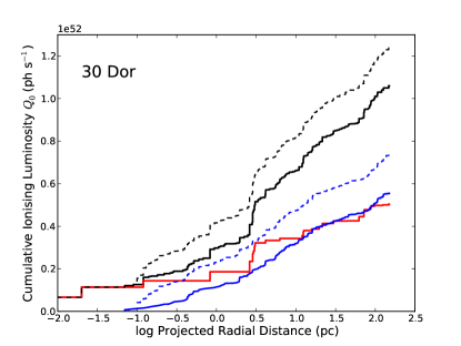
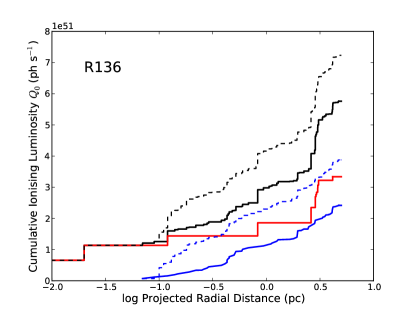
Figure 14: Cumulative ionising luminosities of the hot luminous stars in 30 Dor (a) and the R136 region (b). Feedback from all stars (black), W-R and Of/WN stars (red) and OB stars (blue). Solid lines include the feedback from stars which were spectroscopically classified as hot and luminous (Sp) while dashed lines include feedback from photometrically classified stars (Sp+Ph).

8.2 Stellar wind luminosity and momentum

The total stellar wind luminosity of 30 Dor was estimated at $L_{\mathrm{SW}}^{\mathrm{Sp}}$ $\approx 1.97\times 10^{39}$ erg s^-1. Figure 15 shows the radial cumulative wind luminosity to behave similarly to the ionising luminosity: rapidly increasing within the inner 20 pc from which $\sim 75$% of the total wind luminosity is produced. W-R and Of/WN stars dominate the mechanical output, providing about two thirds of the total. Their higher contribution arises from their high mass-loss rates and fast winds. This behaviour is repeated in the R136 region (see Figure 15), where the four WN 5h stars again provide significant mechanical feedback to the cluster. The dashed lines again represent our combined spectroscopically and photometrically classified sample. $L_{\mathrm{SW}}^{\mathrm{Sp+Ph}}$ values suggest wind luminosities in the R136 region and within 30 Dor could increase roughly a further 25% and 15%, respectively.

Again, we can compare to the work of CrowtherDessart:1998 who found $L_{\mathrm{SW}}=1.61\times 10^{39}\,\mathrm{erg\,s}^{-1}$ out to $r_{\mathrm{d}}=10$ pc, i.e. about 15% higher than our $L_{\mathrm{SW}}^{\mathrm{Sp+Ph}}$ estimate (see Table 9). The offset results again from the updated stellar calibrations and mass-loss rates that are corrected for wind clumping.

Table 10 also lists the ten stars with the highest wind luminosities. These are all W-R stars, most of which overlap with the dominant ionising stars and are also located within the R136 region. The importance of the W-R stars is echoed here as these 10 stars alone contribute 35% of $L_{\mathrm{SW}}^{\mathrm{Sp+Ph}}$. Once again, contributions of subluminous stars become negligible, such as the VFTS O-type stars excluded from our census whose combined wind luminosity is $<0.05$% of $L_{\mathrm{SW}}^{\mathrm{Sp}}$ and just a few % of the B-type star output.

The integrated modified wind momenta, $D_{\mathrm{mom}}$, behave very similarly to $L_{\mathrm{SW}}$. Table 9 shows how the W-R and Of/WN stars are again the key contributors while the contribution from OB stars is slightly reduced, likely due to the lower dependence that their high $\varv_{\infty}$ play on $D_{\mathrm{mom}}$.

We note that the contribution of the W-R stars to the stellar bolometric luminosity is different to the stellar feedback. OB stars contribute $\sim 70$% of the bolometric luminosity of 30 Dor (Table 9). W-R and Of/WN stars, while individually luminous compared to many of the OB stars, contribute $\sim 30$% of the integrated luminosity of the region.

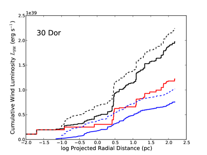
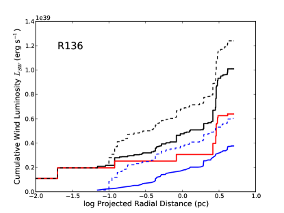
Figure 15: Cumulative stellar wind luminosities of the hot luminous stars in 30 Dor (a) and the R136 region (b). Lines are as in Figure 14.

8.3 Feedback from additional sources

While the census focusses on selecting hot luminous stars, our estimates are potentially influenced by additional sources of feedback. Embedded stars, shock emission and sources outside the census could all contribute. Nevertheless, here we argue that they will only have a limited impact on our integrated values and that the W-R stars still have the greatest influence.

First we address the impact of stars beyond our selected $r_{\mathrm{d}}\leq 150$ pc region of 30 Dor. Figures 14 & 15 clearly show the cumulative effect of hot luminous stars to drop off at large distances from R136. There are no significant young clusters close to our census border to provide extra feedback. Indeed, even if we were to extend our census to $r_{\mathrm{d}}\leq 225$ pc (more than doubling the projected area on the sky), we would only expect to enclose a further $\sim 300$ candidate hot luminous stars (25% of the census). Spectral coverage is poor beyond $r_{\mathrm{d}}\sim 150$ pc but only one W-R star is known, BAT99-85/VFTS 002, WC 4+(O6-6.5 III).

The isochrones in Figure 12 show the age of massive stars within 30 Dor to extend beyond 8 Myr, with ages of 20-25 Myr derived for the Hodge 301 cluster (GrebelChu:2000). This clearly extends well beyond the epoch of the first SNe that would have occurred in the region and is demonstrated by the N157B supernova remnant (Chu:1992). A complex structure of gas filaments and bubbles is generated by stellar winds and SNe, many of which coincide with bright X-ray sources (Townsley:2006). ChuKennicutt:1994. identify a number of gas shells expanding at velocities up to 200 km s^-1. Despite the evidence for shocks, the ionising output from hot stars seems capable of keeping the shells ionised (ChuKennicutt:1994).

A further lack of highly ionised species, such as [O  iv] and [Ne v] leaves photoionisation as the dominant process in the energy budget (Indebetouw:2009; Pellegrini:2010). As neither optical nor IR nebular emission lines show strong correlation between high excitation regions and listed embedded stars, the ionisation structure of 30 Dor primarily arises from the optically known hot stars.

When considering mechanical feedback, however, SNe do become significant. While some of the smaller shells are thought to be wind-blown bubbles, the larger and faster moving shells are only likely to be carved by the energy input of SNe (ChuKennicutt:1994). An exception would be the shell surrounding R136. Taking our derived wind luminosity for the R136 region with a pre-SNe age of $\sim 2$ Myr, the kinetic energy generated by the stellar winds could amount to a few $10^{52}\,\mathrm{erg}$, sufficiently high to drive the bubble (ChuKennicutt:1994). However, determining a combined stellar/SNe energy budget for 30 Dor, awaits a better understanding of its star formation history (SFH).

8.4 R136 comparison with population synthesis models

Population synthesis codes seek to mimic the combined properties of a stellar system of a given age and mass. With only a few initial parameters being required, expected observable properties of extragalactic star forming regions can be predicted. However, there are limited targets available to test the reliability of such models. R136 is one of the few resolved massive star clusters which allows an empirical study of the stars to be compared to synthetic predictions. In particular, its high mass ($M_{\rm{cl}}=5-10\times 10^{4}$ M_⊙, Hunter:1995; Andersen:2009) and young age ($1-2$ Myr, Section 7), means that the upper MF is well populated and stochastic effects are minimal (Cervino:2002).

A synthetic model of an R136-like cluster was generated by the population synthesis code, Starburst99 (Leitherer:1999). An instantaneous burst model with total mass $10^{6}$ M_⊙ and metallicity $Z=0.4\,Z_{\odot}$ was adopted, which was scaled to $M_{\rm{cl}}=5.5\times 10^{4}$ M_⊙, in order to mimic R136. A Kroupa:2001 IMF with $M_{\rm{up}}=100$ M_⊙ was selected along with the “high mass-loss rate” Geneva evolutionary tracks of Meynet:1994. The theoretical wind model was chosen, meaning that the wind luminosity produced was based on mass-loss rates and terminal wind velocities from Equations 1 & 2 of Leitherer:1992, respectively. Ionising luminosities used the calibration from Smith:2002.

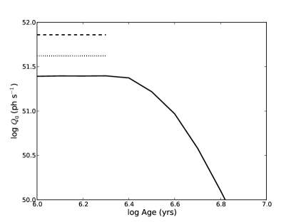
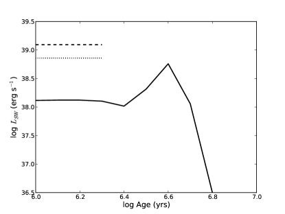
Figure 16: The integrated ionising luminosity (a) and stellar wind luminosity (b) of the R136 region. Predictions from Starburst99 are plotted with a solid line. Values from our census, with and without $M_{\mathrm{init}}>100$ M_⊙ stars, are plotted in dashed and dotted lines, respectively.

Our empirical feedback for R136 is compared with Starburst99 in Figure 16. Here we compare the combined spectroscopic and photometric values ($Q_{\mathrm{0}}^{\mathrm{Sp+Ph}}$ & $L_{\mathrm{SW}}^{\mathrm{Sp+Ph}}$). The Starburst99 predictions only represent contributions from stars (i.e. excluding supernovae). Their changing values, over time, reflect the different SpTs that contribute to the feedback. Comparisons to Starburst99 are made between 1-2 Myr, given the age obtained by MasseyHunter:1998 for the most luminous members of R136 (see also Figure 12). We see that in both cases, our empirical results exceed the predictions of Starburst99. The predicted ionising luminosity underestimates the empirical results by a factor of two, while the wind luminosity is underestimated by a factor of nine.

The standard feedback recipe for Starburst99 is somewhat dated and may help explain this disagreement. In the case of the ionising luminosity, we have seen how W-R stars contribute significantly to the output of R136. Recent spectral modelling of the four core WN 5h stars by Crowther:2010 has estimated all to have initial masses $M_{\rm{init}}>150$ M_⊙. However, the IMF used for Starburst99 was limited to $M_{\mathrm{up}}=100$ M_⊙ and the incorporated evolutionary tracks only extended up to $120$ M_⊙. The Starburst99 output would therefore have excluded stars with $M_{\rm{init}}>100$ M_⊙.

In an attempt to identify other stars with $M_{\rm{init}}>100$ M_⊙, we examined the latest Bonn evolutionary tracks , which extend to $500$ M_⊙. For LMC metallicity and at an age of $\leq 2$ Myr, the luminosity of a $100$ M_⊙ star was expected to be $\log(L_{\mathrm{Bol}}/\mathrm{L}_{\odot})\gtrsim 6.3$. Table 10 lists ten census stars to which this applies, of which eight are located within the R136 region. The dotted lines in Figure 16, show our empirical results if such stars are excluded. A better agreement is obtained with Starburst99, with differences in $Q_{0}$ reduced to $\sim 0.2$ dex. We find minimal differences between our $q_{\mathrm{0}}$ calibration and the one used by Starburst99 (Smith:2002), so this remaining offset most likely arises from the higher $T_{\mathrm{eff}}$ that we assign to our SpTs.

When comparing the wind luminosities, excluding stars with $M_{\rm{init}}>100$ M_⊙ has less of an impact and Starburst99 is still seen to underestimate our empirical results by $\sim 0.7$ dex. In this case, the disagreement largely arises from the different mass-loss prescriptions. Starburst99 predictions follow Leitherer:1992 and are found to differ from the Vink:2001 mass-loss rates by a factor of $2-10$, depending on SpT. Any differences in $\varv_{\infty}$ should be minimal, however, (see Figure 2 in Leitherer:1992).

We note that neither rotation or binarity are accounted for in evolutionary models used in Starburst99. However, more recent versions (Vazquez:2007; Levesque:2012) do attempt to address the effects of rotation on stellar outputs, as well as adopting the Vink:2001 mass-loss prescription. They typically found that rotating models prolonged the ionising output of stars, particularly those in lower mass bins. Rotation led to increased temperatures and luminosities and hence a greater and harder ionising luminosity, especially $>3$ Myr in the presence of W-R stars. Rotational mixing would also increase mass-loss rates and so the wind luminosity is potentially higher as well. The situation is more complex when incorporating massive binaries, but EldridgeStanway:2009 indicate an increase in ionising luminosity at later ages. Despite these updates, the ability to model the most massive stars still appears crucial for accurate predictions of the feedback. Evolutionary models for very massive stars are in the process of being included in synthetic codes .

Table 10: The census stars with the highest ionising luminosities, wind luminosities and masses and their combined contribution to 30 Dor. Entries given in bold are based on tailored W-R analyses (see Table LABEL:tab:W-R_and_Of/WN_star_parameters). Other entries rely either on the less reliable W-R star template method or the calibrations discussed in Section 6. For more reliable outputs for the Of/WN and WN stars, we direct the reader to Bestenlehner et al. .

ID	Star	SpT	$r_{\mathrm{d}}$	$Q_{\mathrm{0}}$	$L_{\mathrm{SW}}$
#			(pc)	($10^{49}$ ph s${}^{-1})$	($10^{37}$erg s-1)
10 STARS WITH HIGHEST IONISING LUMINOSITY
630	R136a1	WN 5h	0.00	66.0	10.9
770	Mk34	WN 5h	2.61	49.2	9.2
633	R136a2	WN 5h	0.02	48.0	8.7
706	R136c	WN 5h	0.83	42.0	5.4
493	R134	WN 6(h)	2.86	35.3	6.2
613	R136a3	WN 5h	0.12	30.0	5.6
1001	BAT99-122	WN 5h	71.71	25.0	5.5
580	Mk 42	O2 If*	1.96	18.8	4.0
916	BAT99-118	WN 6h	62.27	18.2	5.3
375	BAT99-95	WN 7h	21.56	15.8	7.6
Total (% of $Q_{\mathrm{0}}^{\mathrm{Sp+Ph}}$ or $L_{\mathrm{SW}}^{\mathrm{Sp+Ph}}$):				348.3 (28%)	68.4 (29%)
10 STARS WITH HIGHEST WIND LUMINOSITY
630	R136a1	WN 5h	0.00	66.0	10.9
543	R140a1	WC 4	12.43	6.6	9.7
762	Mk33Sb	WC 5	2.90	6.3	9.4
770	Mk34	WN 5h	2.61	49.2	9.2
633	R136a2	WN 5h	0.02	48.0	8.7
375	BAT99-95	WN 7h	21.6	15.8	7.6
493	R134	WN 6(h)	2.86	35.3	6.2
613	R136a3	WN 5h	0.12	30.0	5.6
1001	BAT99-122	WN 5h	71.7	25.0	5.5
706	R136c	WN 5h	0.83	42.0	5.4
Total (% of $Q_{\mathrm{0}}^{\mathrm{Sp+Ph}}$ or $L_{\mathrm{SW}}^{\mathrm{Sp+Ph}}$):				324.2 (28%)	78.2 (35%)
STARS WITH $M_{\rm{init}}>$100 M⊙
630	R136a1	WN 5h	0.00	66.0	10.9
770	Mk34	WN 5h	2.61	49.2	9.2
633	R136a2	WN 5h	0.02	48.0	8.7
706	R136c	WN 5h	0.83	42.0	5.4
493	R134	WN 6(h)	2.86	35.3	6.2
613	R136a3	WN 5h	0.12	30.0	5.6
1001	BAT99-122	WN 5h	71.71	25.0	5.5
580	Mk 42	O2 If*	1.96	18.8	4.0
916	BAT99-118	WN 6h	62.27	18.2	5.3
375	Mk35	O2 If*/WN 5	3.07	15.6	1.7
Total (% of $Q_{\mathrm{0}}^{\mathrm{Sp+Ph}}$ or $L_{\mathrm{SW}}^{\mathrm{Sp+Ph}}$):				348.1 (28%)	62.5 (28%)

9 Star Formation Rates

There are various methods to estimate the SFR of a region, from UV through to IR. Each have advantages and disadvantages, as they trace the fates of the ionising photons from the young stellar population (Kennicutt:1998). Our census of 30 Dor now provides us with the total ionising luminosity produced by its stars. The UV stellar continuum is often used to directly probe this emission while gaseous nebular recombination lines (e.g. H$\alpha$) and the far-infrared (FIR) dust continuum are more widely used. In this section we compare the findings of these different indicators for both Salpeter:1955 and Kroupa:2001 IMFs. Comparing their estimates to those of our census also allows us to determine the possible fraction of ionising photons which may be escaping the region, $f_{\mathrm{esc}}$.

Kennicutt:1998 provide a series of widely used calibrations to estimate the SFR from various wavelengths. They are derived from population synthesis models which predict the respective luminosities ($Q_{\mathrm{0}}$, H$\alpha$ etc.) for a given set of parameters, including the IMF, over a period of constant star formation. They were revisited in a review by KennicuttEvans:2012 and references therein, where changes arose from updates to the IMF and stellar population models. However, these calibrations are more applicable to galaxies and starburst regions, for which star formation has occurred for at least 100 Myr. In the case of 30 Dor, findings from WalbornBlades:1997 and our census suggest stellar ages $>10$ Myr but information on the region’s SFH is limited. Nevertheless, DeMarchi:2011 had used their HST/WFC3 photometry to focus on pre main-sequence stars, albeit within a smaller central region of 30 Dor compared to our census. They estimated a relatively constant SFH for 30 Dor for the past $\sim 10$ Myr.

Based on these findings, we opted to derive our own SFR calibrations using Starburst99. For the case of 30 Dor, our synthetic model was set to run for 10 Myr with a continuous $\mathrm{SFR}=1\,\mathrm{M}_{\odot}\,\mathrm{yr}^{-1}$. All other model parameters were identical to our R136 burst model, i.e. a Kroupa IMF, “high mass-loss rate” Geneva evolutionary tracks and $Z=0.4\,Z_{\odot}$. The calibrations given in Equations 1 - 4 were then derived from the respective luminosities, as predicted by Starburst99, at an age of 10 Myr. However, we showed earlier, the exclusion of $M_{\rm{init}}>100$ M_⊙ stars can lead to integrated stellar luminosities being underestimated. On this occassion, we do not attempt to adjust the coefficients in Equations 1 - 4, noting that the most massive stars could lead to SFR discrepancies. Nevertheless, they should still be more reliable than those calibrated for galaxies.

9.1 Lyman continuum from census

30 Dor offers us the rare opportunity to measure the integrated Lyman continuum (LyC) ionising luminosity directly from its stars. As only massive ($>10$ M_⊙) and young ($<20$ Myr) stars significantly contribute to this quantity, it provides a nearly instantaneous measure of the SFR (Kennicutt:1998). We have already estimated this integrated value as $Q_{\mathrm{0}}^{\mathrm{Sp+Ph}}$. The resulting SFR for 30 Dor is then:

$$\mathrm{SFR}\,(\mathrm{M}_{\odot}\,\mathrm{yr}^{-1})=5.8\times 10^{-54}Q_{\mathrm{0}}\,(\mathrm{ph\,s}^{-1}).$$ (1)

When accounting for photometrically classified stars, the census gives a SFR of 0.105 or 0.073 $\mathrm{M}_{\odot}\,\mathrm{yr}^{-1}$ for a Salpeter or Kroupa IMF, respectively (see Table 9.4). Having accounted for stars individually, this is one of the most direct methods of quantifying their ionising luminosity. We now discuss the alternative methods available and compare their results in Table 9.4.

9.2 Far-UV continuum

Probing the young massive stars can also be achieved in the far-UV (FUV), since they will dominate the integrated UV spectrum of a star forming region. However, it is particularly sensitive to extinction (as the cross-section of dust peaks in the UV). The FUV continuum flux of 30 Dor was obtained from Ultraviolet Imaging Telescope (UIT) images using its B5 (1615 Å) filter (Parker:1998). An aperture, consistent to our census region was used and corrected for a uniform extinction using the Fitzpatrick:1986 law, adopting an average $R_{V}\approx 3.5$ and $E(B-V)\approx 0.4$. Our SFR calibration for 30 Dor from the FUV is:

$$\mathrm{SFR}\,(\mathrm{M}_{\odot}\,\mathrm{yr}^{-1})=1.2\times 10^{-40}L_{1615}\,\mathrm{(erg\,s^{-1}\,\AA^{-1})},$$ (2)

where $L_{1615}$ is the continuum luminosity at 1615 Å. This gave a SFR in very good agreement with the census. As a direct tracer of the hot luminous stars, the consistency of the FUV continuum luminosity would be expected. The sensitivity of this diagnostic to extinction shows that the adoption of a uniform Fitzpatrick:1986 law is reasonable for 30 Dor.

9.3 Lyman continuum from H$\alpha$

For most giant H ii regions, the ionising stars are not individually observable and hydrogen recombination lines, primarily H$\alpha$, serve as the main indicator for a young massive population. Kennicutt:1995 measured the H$\alpha$ flux from 30 Dor through a series of increasing circular apertures, centred on R136, from which we selected a 10 arcmin radius, consistent with our census region. Observations from Pellegrini:2010 gave an integrated nebular flux ratio of $F(\mathrm{H}\alpha)/F(\mathrm{H}\beta)=4.37$. Assuming the intrinsic ratio to be 2.86 for an electron temperature of $T_{\mathrm{e}}=10^{4}$ K and electron density of $n_{\mathrm{e}}=100\,\mathrm{cm}^{-3}$, we find $A_{\mathrm{H\alpha}}=1.20$ mag when applying $R_{V}=3.5$ as before. The SFR for 30 Dor based on H$\alpha$ is then:

$$\mathrm{SFR}\,(\mathrm{M}_{\odot}\,\mathrm{yr}^{-1})=4.2\times 10^{-42}L_{\mathrm{H}\alpha}\,(\mathrm{erg\,s}^{-1})$$ (3)

where $L_{\mathrm{H}\alpha}$ is the H$\alpha$ luminosity. The SFR from this method is $\sim 30$% lower than estimates from the census. As with the FUV, this method can be sensitive to extinction as well as the IMF. Furthermore, absorption of ionising photons by dust and their potential leakage make this SFR a lower limit.

9.4 Far-infrared continuum

Stellar UV photons may be absorbed by dust and re-emitted at FIR wavelengths. Measuring the FIR luminosity ($L_{\mathrm{FIR}}$) allows us to account for this absorption and in cases of high dust opacity, it provides a SFR tracer too. Skibba:2012 recently produced dust luminosity ($L_{\mathrm{dust}}$) surface density maps of the Magellanic Clouds. These integrated observations from the Spitzer SAGE (Meixner:2006) and Herschel Space Observatory HERITAGE surveys. $L_{\mathrm{dust}}$ covered 5.8-500 $\mu$m, and while limits are not completely consistent with the FIR provided by Starburst99, the FIR peak ($\sim 100\mu$m) is well covered and the overall difference should be small. Our equivalent SFR calibration for 30 Dor in the FIR is:

$$\mathrm{SFR}\,(\mathrm{M}_{\odot}\,\mathrm{yr}^{-1})=4.2\times 10^{-44}L_{\mathrm{FIR}}\,(\mathrm{erg\,s}^{-1}),$$ (4)

where $L_{\mathrm{FIR}}$ refers to the far infrared luminosity. The coefficient is based on the total bolometric luminosity of the stars as predicted by Starburst99, assuming that all of the stellar luminosity is absorbed and re-radiated by the dust. The FIR continuum implies a SFR significantly lower (factor of $\sim 10$) than our census. This would indicate that only a small proportion of the ionising photons contribute to heating the dust with the remainder either ionising gas or escaping the region. It should also be noted that older stellar populations $(>10$ Myr) are still capable of heating the dust and contributing to the FIR emission, even if they no longer produce ionising photons. Such stars are not related to the recent star formation.

Table 11: Comparison of SFR tracers for 30 Dor.

SFR Tracer			SFR [M⊙ y$r^{-1}$]
			Salpeter IMF	Kroupa IMF
Lyman Continuum (Stars)	$F_{1615}$ [erg cm-2 s-1 Å]	$4.88\times 10^{-11}$			$Q_{\mathrm{0}}^{\mathrm{Sp+Ph}}$ [ph s-1]	$12.37\times 10^{51}$	$0.103\pm 0.062$	$0.073\pm 0.044$ FUV Continuum (1615Å)
	$I_{1615}$erg cm-2 s-1 Å]	$2.01\times 10^{-9}$
	$F_{\mathrm{H}\alpha}$ [erg cm-2 s-1]	$1.37\times 10^{-8}$
$I_{\mathrm{H}\alpha(\mathrm{corr})}$erg cm-2 s-1]	$4.12\times 10^{-8}$
$F_{22}$ [Jy]	2800
$\nu L_{22}$ [erg s-1]	$1.13\times 10^{41}$
$L_{\mathrm{FIR}}$ [erg s-1]	$1.58\times 10^{41}$	$0.010\pm 0.001$	$0.007\pm 0.001$	$L_{\mathrm{H}\alpha(\mathrm{corr})}$ [erg s-1]	$1.23\times 10^{40}$	$0.100\pm 0.018$	$0.070\pm 0.012$ FIR Continuum

9.5 Combined H$\alpha$ and mid-IR

By combining a dust-emission-based tracer with one tracing ionised gas, it should be possible to account for all the ionising photons, except for those escaping the region. Calzetti:2007 and Kennicutt:2009 provide such a SFR diagnostic by combining the observed H$\alpha$ and 24 $\mu$m luminosities. The observed H$\alpha$ luminosity was calculated from Kennicutt:1995 as before, only not corrected for extinction. Spitzer 24 $\mu$m observations were unfortunately saturated at the core of 30 Dor. We therefore turned to the similar 22 $\mu$m filter aboard the Wide-field Infrared Survey Explorer (WISE), and measured a luminosity from the archival image coadd_id=0837m697_ab41. While the SFR calibration of Calzetti:2007 is suited for H ii regions (their Equation 7), for consistency we replace their first coefficient with the one derived in our Equation 3. In addition, to account for the narrower bandwidth and shorter wavelength of the WISE filter, their second coefficient was adjusted to give:

$$\mathrm{SFR}\,(\mathrm{M}_{\odot}\,\mathrm{yr}^{-1}) = 4.2\times 10^{-42}[L_{\mathrm{H}\alpha(\mathrm{obs})}\,(\mathrm{erg\,s}^{-1})$$ (5)

$$+0.039\times\nu L_{22}\,(\mathrm{erg\,s}^{-1})],$$

where $L_{22}$ is the observed luminosity density at $22\,\mu$m and $\nu$ is the central frequency of the $22\,\mu$m filter. This method also estimated a SFR lower than our empirical census, by a factor of $\sim 2$. However, we note that by substituting the extinction corrected H$\alpha$ luminosity ($L_{\mathrm{H}\alpha(\mathrm{corr})}$) into Equation 5, results are much more consistent. This approach would therefore be recommended for star forming regions lacking UV imaging.

9.6 Photon escape fraction

The leakage of ionising photons from 30 Dor might be expected given the open structure and filaments of the region. We can only consider the $f_{\mathrm{esc}}$ for 30 Dor by dealing in numbers of photons. We have already determined the number of ionising photons emitted by its stars, $Q_{\mathrm{0}}^{\mathrm{Sp+Ph}}$. The number of photons which ionise the gas ($Q_{\mathrm{0}}^{\mathrm{H}\alpha}$) can be calculated from Equations 1 and 3, and is shown to be directly proportional to $L(\mathrm{H}\alpha)$.

The number of photons absorbed by dust ($Q_{\mathrm{0}}^{\mathrm{Dust}}$) is more complicated since both EUV and non-EUV photons contribute to heating the dust. We therefore use the $L_{\mathrm{EUV}}/L_{\mathrm{Bol}}$ fraction which was estimated for each SpT (see Tables 5 - 8) using the models of Martins:2005 and DoranCrowther:2011. We obtain an average $L_{\mathrm{EUV}}/L_{\mathrm{Bol}}\approx 0.45$ for 30 Dor as a whole, representing a typical O5 V star. If we were to apply this same fraction to the dust then $L^{\mathrm{Dust}}_{\mathrm{EUV}}\sim 0.45\times L_{\mathrm{FIR}}$, where $L^{\mathrm{Dust}}_{\mathrm{EUV}}$ is the dust luminosity heated by EUV photons. Of course, we have already determined that a fraction of the EUV photons leaving our stars must ionise the gas, while variations in the dust opacity could result in further photons escaping the region. An additional test was therefore made with the grain models of WeingartnerDraine:2001 to calculate the fraction of ionising luminosity of a typical O5 V star, that is absorbed by dust. These estimates suggested that $L^{\mathrm{Dust}}_{\mathrm{EUV}}\approx 0.55\times L_{\mathrm{EUV}}$ for a variety of $R_{V}$ values . Therefore, in terms of the number of ionising EUV photons:

$$Q_{\mathrm{0}}^{\mathrm{Dust}}\sim 0.55\times L_{\mathrm{FIR}}/L_{\mathrm{EUV}}\times Q_{\mathrm{0}}^{\mathrm{Sp+Ph}}.$$ (6)

Table LABEL:tab:Photon_Escape_Fraction gives a breakdown of the ionising photons. The ratio of $(Q_{\mathrm{0}}^{\mathrm{H\alpha}}+Q_{\mathrm{0}}^{\mathrm{Dust}})/Q_{\mathrm{0}}^{\mathrm{Sp+Ph}}\sim 0.94$, therefore $f_{\mathrm{esc}}\sim 0.06$. This would suggest 30 Dor to be ‘density bounded’ with just under 6% of its ionising photons escaping the region. Given the uncertainties on our values, $f_{\mathrm{esc}}$ potentially ranges from $0-0.61$. This could equally see 30 Dor as a ‘radiation bounded’ region. However, we recall that $Q_{\mathrm{0}}^{\mathrm{Sp+Ph}}$ is still likely an underestimate due to unaccounted contributors (see Section 5.3). $Q_{\mathrm{0}}^{\mathrm{Dust}}$ is also likely to be an upper limit. This arises from the omission of luminous cool supergiants from the census due to their minimal ionising luminosity. However, these older stellar populations would still have contributed to $L_{\mathrm{Bol}}$, hence lowering the integrated $L_{\mathrm{EUV}}/L_{\mathrm{Bol}}$ fraction.

SmithBrooks:2007 followed the same approach as our work on the Carina Nebula and found a quarter and one third of the ionising photons to be unaccounted for when comparing to radio and H$\alpha$ fluxes, respectively. Similar work by Voges:2008 showed 20-30% of their less luminous LMC H ii regions to be in a similar density bounded state. A slightly different approach was made by Pellegrini:2011b who implemented nebular line ratios to detect ionisation fronts around H ii regions in the Magellanic Clouds. They too, concluded the regions to be density bounded with average $f_{\mathrm{esc}}>0.4$.

SpT is amended from WN 3o to WN 3(h) following further inspection of the Pickering series. Based on $W_{\lambda}$ dilution of C iv $\lambda 5808$ line. $W_{\lambda}$ of C iv $\lambda 4650$ line (undiluted $W_{\lambda}(4650)\approx 1200$) based on BAT99-90. Revealed as a WN 5-6+WN 6-7 binary system by Sana:2013b $M^{\mathrm{sys}}_{v}$ was estimated using broad band photometry and $v-\mathrm{V}\approx 0.2$ mag relation from Breysacher:1986. However, high reddening allows for a large uncertainty and the star is thought to be more comparable to BAT99-106 (F. Najarro).

Appendix C Reddening

A recent tailored analysis, based on the VFTS O-type stars, indicates a varied amount of extinction across the different regions of 30 Dor . For now we apply a uniform reddening value of $R_{V}=3.5$ within the MEDUSA region and $R_{V}=4.2$ within the R136 region. These values were derived using additional $K$-band photometry of the census stars, VLT-MAD observations from Campbell:2010 supplying the R136 region and the InfraRed Survey Facility (IRSF, see Table 6 of Paper I) supplying other stars. MartinsPlez:2006 offer a $(V-K)_{\mathrm{o}}$ calibration for O-type stars allowing an expected $M_{V}$ to be derived from the $K$-band photometry. This $K$-band derived $M_{V}$ would become consistent with the conventionally derived $M_{V}$ from optical photometry, at an average $R_{V}$ value.

For both regions, a $K$-band extinction of $A_{K}=0.17$ mag was adopted. Figure 26 compares the $K$-band derived $M_{V}$ ($M^{\mathrm{VLT-MAD}}_{V}$) in the R136 region to the $M_{V}$ from the original HST/WFC3 photometry of DeMarchi:2011 ($M^{\mathrm{WFC3}}_{V}$). In theory, both values would be equal with all points falling on the 1:1 relationship line. Despite some scattering, most likely where VLT-MAD photometry became less reliable in the core, a value of $R_{V}=4.2$ was favoured within R136. In the case of the MEDUSA region (Figure 26), only known single VFTS O-type stars were used in the comparison. The $K$-band derived $M_{V}$ ($M^{\mathrm{IRSF}}_{V}$) was compared to the $M_{V}$ from the original VFTS photometry ($M_{V}^{\mathrm{VFTS}}$), i.e. using Selman, WFI, Parker or CTIO photometry, and favoured a lower value of $R_{V}=3.5$.

An equivalent narrowband $R_{v}$ was required to match the photometry of the W-R stars. We determined this using Equation 24 of SchmutzVacca:1991.

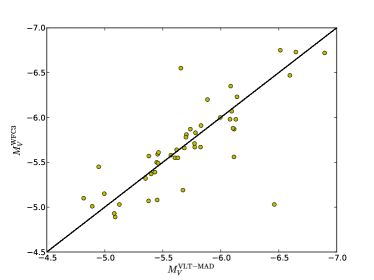
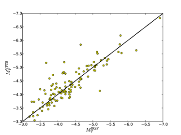
Figure 26: Determination of $R_{V}$ for 30 Dor. In the R136 region (a): The $M_{V}$ of single O-type stars derived from HST/WFC3 photometry is plotted against the expected $M_{V}$ derived from VLT-MAD $K$-band photometry after applying the MartinsPlez:2006 calibration. In the MEDUSA region (b): The $M_{V}$ derived from VFTS photometry is plotted against the expected $M_{V}$ derived from IRSF $K$-band photometry after applying the MartinsPlez:2006 calibration. Solid lines indicate the 1:1 relations.

Appendix D The Census

Table 17: The candidate hot luminous stars in the census as selected by the criteria explained in Section 3. Stars are listed in order of increasing right ascension. The first 20 candidate stars are given here, see online data for full census. References for the photometry are as follows: dM - DeMarchi:2011, S - Selman, W - WFI, P - Parker, C - CTIO, Z - Zaritsky:2004 and Wal - Walborn:1999. Popular aliases are also included from the following catalogues: VFTS - Paper I, HSH95 - Hunter:1995, S99 - Selman:1999, P93 - Parker:1993, ST92 - SchildTestor:1992 and Sk - Sanduleak:1970 catalogues.

ID	$\alpha$	$\delta$	$V$	$B-V$	Ref.	VFTS	HSH95	S99	P93	ST92	Sk
#	(h m s)	$(^{\circ}\,{}^{\prime}\,{}^{\prime\prime})$	(mag)	(mag)
1	05 36 51.12	$-69$ 05 12.20	16.63	$0.67$	W	-	-	-	-	-	-
2	05 36 53.82	$-69$ 04 30.13	17.00	$0.32$	W	-	-	-	-	-	-
3	05 36 55.98	$-69$ 07 36.70	17.36	$0.61$	W	-	-	-	-	-	-
4	05 36 56.85	$-69$ 05 59.36	17.98	$0.68$	W	-	-	-	-	-	-
5	05 36 57.18	$-69$ 08 47.40	15.85	$0.04$	W	-	-	-	-	-	-
6	05 36 57.22	$-69$ 07 23.33	18.33	$0.80$	W	-	-	-	-	-	-
7	05 36 57.26	$-69$ 05 00.01	15.11	$0.69$	W	-	-	-	-	-	-
8	05 36 57.62	$-69$ 03 44.04	14.56	$0.61$	W	-	-	-	-	-	-
9	05 36 58.95	$-69$ 08 21.66	15.33	$0.01$	W	-	-	-	-	-	-
10	05 37 03.59	$-69$ 10 22.32	16.71	$0.32$	W	-	-	-	-	-	-
11	05 37 03.91	$-69$ 10 03.60	13.01	$0.20$	Z	-	-	-	-	-	-
12	05 37 04.01	$-69$ 08 23.83	14.36	$0.80$	W	-	-	-	-	-	-
13	05 37 04.26	$-69$ 08 05.46	16.18	$0.11$	W	009	-	-	-	-	-
14	05 37 04.47	$-69$ 04 00.08	15.56	$0.20$	W	-	-	-	-	-	-
15	05 37 05.63	$-69$ 09 12.20	15.83	$0.15$	W	012	-	-	-	-	-
16	05 37 06.29	$-69$ 04 41.20	16.36	$0.13$	W	013	-	-	-	-	-
17	05 37 08.72	$-69$ 04 45.51	17.36	$0.47$	W	-	-	-	-	-	-
18	05 37 08.88	$-69$ 07 20.39	13.55	$0.04$	Z	016	-	-	-	-	-
19	05 37 09.68	$-69$ 02 21.39	15.88	$-0.02$	W	-	-	-	-	-	-
20	05 37 10.17	$-69$ 05 24.10	17.29	$0.37$	W	-	-	-	-	-	-

Table 18: Stellar parameters of the spectroscopically confirmed hot luminous stars in the census. Absolute magnitudes are given in narrow band for W-R stars and broad band in all other cases. Stars are listed in order of increasing projected distance ($r_{\mathrm{d}}$) from star R136a1. The first 20 stars are given here, see online data for full census. References for the spectral types are are as follows: ST92 - SchildTestor:1992, P93 - Parker:1993, WB97 - WalbornBlades:1997, MH98 - MasseyHunter:1998, CD98 - CrowtherDessart:1998, B99 - Bosch:1999, W99 - Walborn:1999, BAT99 - Breysacher:1999, Paper I - Evans:2011, T11 - Taylor:2011, D11 - Dufton:2011, CW11 - CrowtherWalborn:2011, HB12 - Henault-Brunet:2012a , Walborn - Walborn et al. , McEvoy - McEvoy et al. and this work. Details of the derivation of the stellar parameters can be found in Section 6.

ID	$r_{\mathrm{d}}$	Spectral	Ref.	$T$	$M_{v}$ or $M_{V}$	$\log L$	$Q_{\mathrm{0}}$	$\varv_{\infty}$	$\dot{M}$	$L_{\mathrm{SW}}$	$D_{\mathrm{mom}}$
#	(pc)	Type		(kK)	(mag)	$(\mathrm{L}_{\odot})$	(ph s-1)	(km s-1)	($\mathrm{M}_{\odot}$ yr-1)	(erg s-1)	(g cm${}^{\frac{3}{2}}$ s-2)
630	0.00	WN 5h	CW11	53	$-8.3$	6.9	6.6e+50	2600	5.0e-05	1.1e+38	1.3e+36
633	0.02	WN 5h	CW11	53	$-7.8$	6.8	4.8e+50	2450	5.0e-05	8.7e+37	1.0e+36
642	0.07	O2 If*	CW11	46	$-6.3$	6.1	7.4e+49	3000	5.0e-06	1.3e+37	9.6e+34
638	0.09	O3 III(f*)	MH98	47	$-5.7$	5.8	4.6e+49	3200	2.5e-06	8.4e+36	5.0e+34
640	0.12	O3 V	MH98	48	$-5.5$	5.8	3.9e+49	3000	2.0e-06	5.1e+36	3.0e+34
613	0.12	WN 5h	CW11	53	$-7.4$	6.6	3.0e+50	2200	4.0e-05	5.6e+37	6.5e+35
651	0.14	O3 III(f*)	MH98	47	$-5.5$	5.8	3.9e+49	3200	2.0e-06	6.8e+36	3.8e+34
614	0.15	O7 V	MH98	38	$-6.2$	5.8	2.5e+49	2300	1.6e-06	2.8e+36	2.7e+34
656	0.18	O3 V	CD98	48	$-5.6$	5.9	4.5e+49	3000	2.0e-06	6.2e+36	3.8e+34
595	0.19	O5:: V	MH98	42	$-4.9$	5.4	1.3e+49	2700	4.0e-07	1.0e+36	6.1e+33
602	0.22	O3 V	MH98	48	$-5.9$	6.0	5.6e+49	3000	3.2e-06	8.3e+36	5.4e+34
662	0.25	O9 V	MH98	34	$-5.1$	5.2	3.9e+48	1500	3.2e-07	2.3e+35	2.8e+33
661	0.26	O3-6 V	MH98	44	$-5.5$	5.7	2.9e+49	3000	1.3e-06	3.2e+36	2.0e+34
644	0.28	O3 V	MH98	48	$-5.5$	5.8	4.0e+49	3000	2.0e-06	5.1e+36	3.0e+34
670	0.29	O3 III(f*)	MH98	47	$-5.5$	5.8	3.9e+49	3200	2.0e-06	6.8e+36	3.8e+34
682	0.38	O3 If*	MH98	42	$-6.1$	5.9	4.7e+49	3700	2.0e-06	8.3e+36	4.8e+34
624	0.41	O3 V	MH98	48	$-5.7$	5.9	4.8e+49	3000	2.5e-06	6.8e+36	4.3e+34
678	0.43	O3 III(f*)	MH98	47	$-5.7$	5.9	4.9e+49	3200	2.5e-06	8.9e+36	5.3e+34
687	0.43	O3III (f*)	CD98	47	$-6.2$	6.0	7.1e+49	3200	4.0e-06	1.4e+37	9.1e+34
648	0.44	O3 V	MH98	48	$-5.6$	5.8	4.4e+49	3000	2.0e-06	5.9e+36	3.6e+34