Guiding Designs of Self-Organizing Swarms: Interactive and Automated Approaches

Abstract

Self-organization of heterogeneous particle swarms is rich in its dynamics but hard to design in a traditional top-down manner, especially when many types of kinetically distinct particles are involved. In this chapter, we discuss how we have been addressing this problem by (1) utilizing and enhancing interactive evolutionary design methods and (2) realizing spontaneous evolution of self-organizing swarms within an artificial ecosystem.

1 Introduction

Engineering design has traditionally been a top-down process in which a designer shapes, arranges and combines various components in a specific, precise, hierarchical manner, to create an artifact that will behave deterministically in an intended way Minai et al., (2006); Pahl et al., (2007). However, this process does not apply to complex systems that show self-organization, adaptation and emergence. Complex systems consist of a massive amount of simpler components that are coupled locally and loosely, whose behaviors at macroscopic scales emerge partially stochastically in a bottom-up way. Such emergent properties of complex systems are often very robust and dynamically adaptive to the surrounding environment, indicating that complex systems bear great potential for engineering applications Ottino, (2004).

In an attempt to design engineered complex systems, one of the most challenging problems has been how to bridge the gap between macro and micro scales. Some mathematical techniques make it possible to analytically show such macro-micro relationships in complex systems (e.g., those developed in statistical mechanics and condensed matter physics Bar-Yam, (2003); Boccara, (2010)). However, those techniques are only applicable to “simple” complex systems, in which: system components are reasonably uniform and homogeneous, their interactions can be approximated without losing important dynamical properties, and/or the resulting emergent patterns are relatively regular so that they can be characterized by a small number of macroscopic order parameters Bar-Yam, (2003); Doursat et al., (2012). Unfortunately, such cases are exceptions in a vast, diverse, and rather messy compendium of complex systems dynamics Camazine, (2003); Sole and Goodwin, (2008). To date, the only generalizable methodology available for predicting macroscopic properties of a complex system from microscopic rules governing its fundamental components is to conduct experiments—either computational or physical—to let the system show its emergent properties by itself (Fig. 1, top).

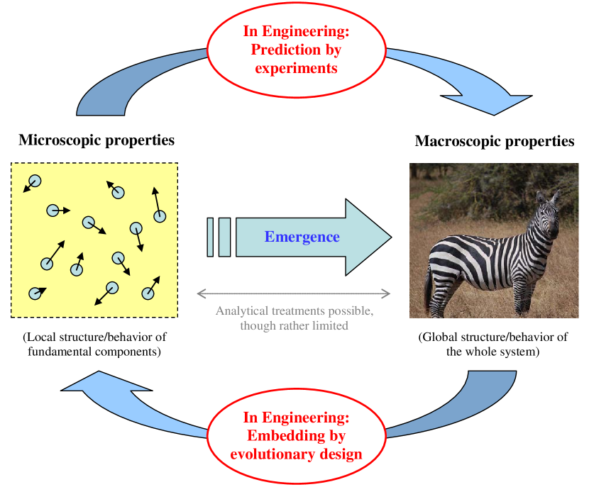
Figure 1: Relationships of macroscopic and microscopic properties in complex systems and how complex systems engineering has been handling the gap between them.

More importantly, the other way of connecting the two scales—embedding macroscopic requirements the designer wants into microscopic rules that will collectively achieve those requirements—is by far more difficult. This is because the mapping between micro and macro scales is highly nonlinear, and also the space of possible microscopic rules is huge and thus hard to explore. So far, the only generalizable methodology available for macro-to-micro embedding in this context is to acquire microscopic rules by evolutionary means Bentley, (1999) (Fig. 1, bottom). Instead of trying to derive local rules analytically from global requirements, evolutionary methods let better rules spontaneously arise and adapt to meet the requirements, even though they do not produce any understanding of the macro-micro relationships. The effectiveness of such “blind” evolutionary search Dawkins, (1996) for complex systems design is empirically supported by the fact that it has been the primary mechanism that has produced astonishingly complex, sophisticated, highly emergent machinery in the history of real biological systems.

The combination of these two methodologies—experiment and evolution—that connect macro and micro scales in two opposite directions (the whole cycle in Fig. 1) is now a widely adopted approach for guiding systematic design of self-organizing complex systems Minai et al., (2006); Anderson, (2006). Typical design steps are to (a) create local rules randomly or using some heuristics, (b) conduct experiments using those local rules, (c) observe what kind of macroscopic patterns emerge out of them, (d) select and modify successful rules according to the observations, and (e) repeat these steps iteratively to achieve evolutionary improvement of the microscopic rules until the whole system meets the macroscopic requirements.

Such experiment-and-evolution-based design of complex systems is not free from limitations, however. In typical evolutionary design methods, the designer needs to explicitly define a performance metric, or “fitness”, of design candidates, i.e., how good a particular design is. Such performance metrics are usually based on relatively simple observables easily extractable from experimental results (e.g., the distance a robot traveled, etc.). However, simple quantitative performance metrics may not be suitable or useful in evolutionary design of more complex structures or behaviors, such as those seen in real-world biological systems, where the key properties a system should acquire could be very diverse and complex, more qualitative than quantitative, and/or even unknown to the designer herself beforehand.

In this chapter, we present our efforts to address this problem, by (1) utilizing and enhancing interactive evolutionary design methods and (2) realizing spontaneous evolution of self-organizing swarms within an artificial ecosystem.

2 Model: Swarm Chemistry

We use Swarm Chemistry Sayama, (2007, 2009) as an example of self-organizing complex systems with which we demonstrate our design approaches. Swarm Chemistry is an artificial chemistry Dittrich et al., (2001) model for designing spatio-temporal patterns of kinetically interacting heterogeneous particle swarms using evolutionary methods. A swarm population in Swarm Chemistry consists of a number of simple particles that are assumed to be able to move to any direction at any time in a two- or three-dimensional continuous space, perceive positions and velocities of other particles within its local perception range, and change its velocity in discrete time steps according to the following kinetic rules (adopted and modified from the rules in Reynolds’ Boids Reynolds, (1987); see Fig. 2):

• If there are no other particles within its local perception range, steer randomly (Straying).

• Otherwise:

  • Steer to move toward the average position of nearby particles (Cohesion, Fig. 2(a)).

  • Steer toward the average velocity of nearby particles (Alignment, Fig. 2(b)).

  • Steer to avoid collision with nearby particles (Separation, Fig. 2(c)).

  • Steer randomly with a given probability (Randomness).

• Approximate its speed to its own normal speed (Self-propulsion).

These rules are implemented in a simulation algorithm that uses kinetic parameters listed and explained in Table 1 (see Sayama, (2009, 2010) for details of the algorithm). The kinetic interactions in our model uses only one omni-directional perception range ($R^{i}$), which is much simpler than other typical swarm models that use multiple and/or directional perception ranges Reynolds, (1987); Couzin et al., (2002); Kunz and Hemelrijk, (2003); Hemelrijk and Kunz, (2005); Cheng et al., (2005); Newman and Sayama, (2008). Moreover, the information being shared by nearby particles is nothing more than kinetic one (i.e., relative position and velocity), which is externally observable and therefore can be shared without any specialized communication channels. These features make this system uniquely simple compared to other self-organizing swarm models.

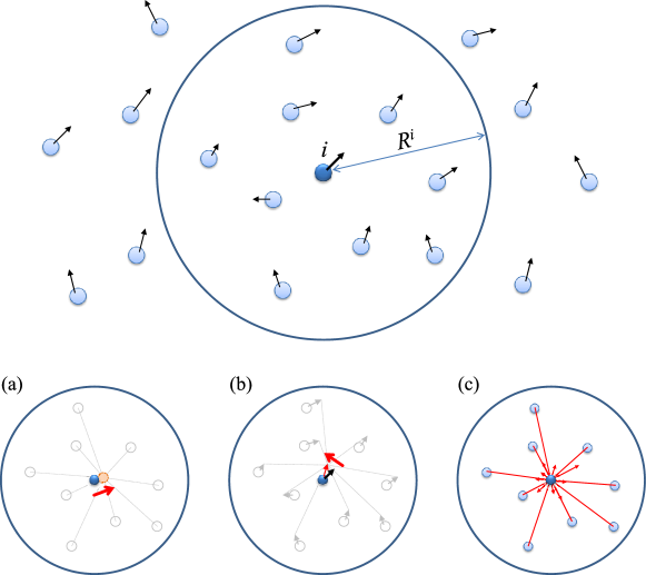
Figure 2: Kinetic interactions between particles (from Sayama, (2010)). Top: Particle $i$ senses only positions and velocities of nearby particles within distance $R^{i}$. Bottom: (a) Cohesion. Particle $i$ accelerates toward the center of mass of nearby particles. (b) Alignment. Particle $i$ steers to align its orientation to the average orientation of nearby particles. (c) Separation. Particle $i$ receives repulsion forces from each of the nearby particles whose strength is inversely related to distance.

Table 1: Kinetic parameters involved in the simulation of particle behavior (from Sayama, (2010)). Unique values are assigned to these parameters for each particle $i$ as its own kinetic properties.

Name	Min	Max	Meaning	Unit
$R^{i}$	0	300	Radius of local perception range	pixel
$V^{i}_{n}$	0	20	Normal speed	pixel step-1
$V^{i}_{m}$	0	40	Maximum speed	pixel step-1
$c^{i}_{1}$	0	1	Strength of cohesive force	step-2
$c^{i}_{2}$	0	1	Strength of aligning force	step-1
$c^{i}_{3}$	0	100	Strength of separating force	pixel2 step-2
$c^{i}_{4}$	0	0.5	Probability of random steering	—
$c^{i}_{5}$	0	1	Tendency of self-propulsion	—

Each particle is assigned with its own kinetic parameter settings that specify preferred speed, local perception range, and strength of each kinetic rule. Particles that share the same set of kinetic parameter settings are considered of the same type. Particles do not have a capability to distinguish one type from another; all particles look exactly the same to themselves.

For a given swarm, specifications for its macroscopic properties are indirectly and implicitly woven into a list of different kinetic parameter settings for each swarm component, called a recipe (Fig. 3) Sayama, (2009). It is quite difficult to manually design a specific recipe that produces a desired structure and/or behavior using conventional top-down design methods, because the self-organization of a swarm is driven by complex interactions among a number of kinetic parameters that are intertwined with each other in highly non-trivial, implicit ways.

97 * (226.76, 3.11, 9.61, 0.15, 0.88, 43.35, 0.44, 1.0) 38 * (57.47, 9.99, 35.18, 0.15, 0.37, 30.96, 0.05, 0.31) 56 * (15.25, 13.58, 3.82, 0.3, 0.8, 39.51, 0.43, 0.65) 31 * (113.21, 18.25, 38.21, 0.62, 0.46, 15.78, 0.49, 0.61)

Figure 3: Example of a recipe, formatted as a list of kinetic parameter sets of different types within a swarm (from Sayama, (2010)). Each row represents one type, which has a number of particles of that type at the beginning, followed by its parameter settings in the format of $(R^{i},V^{i}_{n},V^{i}_{m},c^{i}_{1},c^{i}_{2},c^{i}_{3},c^{i}_{4},c^{i}_{5})$.

In the following sections, we address this difficult design problem using evolutionary methods. Unlike in other typical evolutionary search or optimization tasks, however, in our swarm design problem, there is no explicit function or algorithm readily available for assessing the quality (or fitness) of each individual design. To meet with this unique challenge, we used two complementary approaches: The interactive approach, where human users are actively involved in the evolutionary design process, and the automated approach, where spontaneous evolutionary dynamics of artificial ecosystems are utilized as the engine to produce creative self-organizing patterns.

3 Interactive Approach

The first approach is based on interactive evolutionary computation (IEC) Banzhaf, (2000); Takagi, (2001), a derivative class of evolutionary computation which incorporates interaction with human users. Most IEC applications fall into a category known as “narrowly defined IEC” (NIEC) Takagi, (2001), which simply outsources the task of fitness evaluation to human users. For example, a user may be presented with a visual representation of the current generation of solutions and then prompted to provide fitness information about some or all of the solutions. The computer in turn uses this fitness information to produce the next generation of solutions through the application of a predefined sequence evolutionary operators.

Our initial work, Swarm Chemistry 1.1 Sayama, (2007, 2009), also used a variation of NIEC, called Simulated Breeding Unemi, (2003). This NIEC-based application used discrete, non-overlapping generation changes. The user selects one or two favorable swarms out of a fixed number of swarms displayed, and the next generation is generated out of them, discarding all other unused swarms. Selecting one swarm creates the next generation using perturbation and mutation. Selecting two swarms creates the next generation by mixing them together (similar to crossover, but this mixing is not genetic but physical). Figure 4 shows some examples of self-organizing swarms designed using Swarm Chemistry 1.1.

“swinger”	“rotary”	“walker-follower”

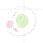
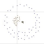
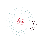
Figure 4: Examples of swarms designed using IEC methods. Their recipes are available on the Swarm Chemistry website (http://bingweb.binghamton.edu/~sayama/SwarmChemistry/).

As a design tool, NIEC has some disadvantages. One set of disadvantage stems from the confinement of the user to the role of selection operator (Fig. 5, left). Creative users who are accustomed to a more highly involved design process may find the experience to be tedious, artificial, and frustrating. Earlier literature suggests that it is important to instill in the user a strong sense of control over the entire evolutionary process Bentley and O’Reilly, (2001) and that the users should be the initiators of actions rather than simply responding to prompts from the system Shneiderman et al., (2009).

These lines of research suggest that enhancing the level of interaction and control of IEC may help the user better guide the design process of self-organizing swarms. Therefore, we developed the concept of hyperinteractive evolutionary computation (HIEC) Bush and Sayama, (2011), a novel form of IEC in which a human user actively chooses when and how to apply each of the available evolutionary operators, playing the central role in the control flow of evolutionary search processes (Fig. 5, right). In HIEC, the user directs the overall search process and initiates actions by choosing when and how each evolutionary operator is applied. The user may add a new solution to the population through the crossover, mutate, duplicate, or random operators. The user can also remove solutions with the delete operator. This naturally results in dynamic variability of population size and continuous generation change (like steady-state strategies for genetic algorithms).

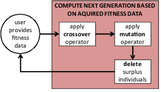
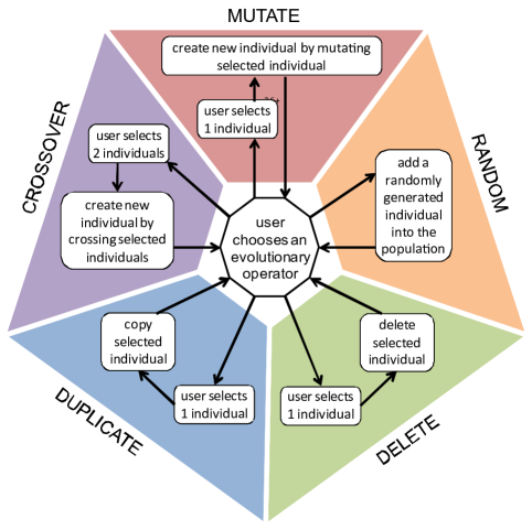
NIEC	HIEC

Figure 5: Comparison of control flows between two interactive evolutionary computation (IEC) frameworks (from Bush and Sayama, (2011)). Left: Narrowly defined IEC (NIEC). Right: Hyper-interactive IEC (HIEC).

We developed Swarm Chemistry 1.2 Sayama et al., (2009); Bush and Sayama, (2011), a redesigned HIEC-based application for designing swarms. This version uses continuous generation changes, i.e., each evolutionary operator is applied only to part of the population of swarms on a screen without causing discrete generation changes. A mutated copy of an existing swarm can be generated by either selecting the “Mutate” option or double-clicking on a particular swarm. Mixing two existing swarms can be done by single-clicking on two swarms, one after the other. The “Replicate” option creates an exact copy of the selected swarm next to it. One can also remove a swarm from the population by selecting the “Kill” option or simply closing the frame. More details of HIEC and Swarm Chemistry 1.2 can be found elsewhere Sayama et al., (2009); Bush and Sayama, (2011).

We conducted the following two human-subject experiments to see if HIEC would produce a more controllable and positive user experience, and thereby better swarm design outcomes, than those with NIEC.

3.1 User experience

In the first experiment, individual subjects used the NIEC and HIEC applications mentioned above to evolve aesthetically pleasing self-organizing swarms. We quantified user experience outcomes using questionnaire, in order to quantify potential differences in user experience between the two applications.

Twenty-one subjects were recruited from students and faculty/staff members at Binghamton University. Each subject was recruited and participated individually. The subject was told to spend five minutes using each of two applications to design an “interesting and lifelike” swarm. Each of these two applications ran on their own dedicated computer station. After completing two sessions, each of which used either NIEC or HIEC application, the subject filled out a survey, rating each of the two platforms on the following factors: easiness of operation, controllability, intuitiveness, fun factor, fatigue level, final design quality, and overall satisfaction. Each factor was rated on a 5-point scale.

The results are shown in Fig. 6. Of the 7 factors measured, 3 showed statistically significant difference between two platforms: controllability, fun factor, and overall satisfaction. The higher controllability ratings for HIEC suggest that our original intention to re-design an IEC framework to grant greater control to the user was successful. Our results also suggest that this increased control may be associated with a more positive user experience, as is indicated by the higher overall satisfaction and fun ratings for HIEC. In the meantime, there was no significant difference detected in terms of perceived final design quality. This issue is investigated in more detail in the following second experiment.

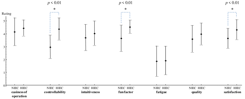
Figure 6: Comparison of rating distribution between the NIEC and HIEC applications across seven factors. Mean ratings are shown by diamonds, with error bars around them showing standard deviations. Significant differences are indicated with an asterisk and corresponding $t$-test $p$-values.

3.2 Design quality

The goal of the second experiment was to quantify the difference between HIEC and NIEC in terms of final design quality. In addition, the effects of mixing and mutation operators on the final design quality were also studied. The key feature of this experiment was that design quality was rated not individually by the subjects who designed them, but by an entire group of individual subjects. The increased amount of rating information yielded by this procedure allowed us to more effectively detect differences in quality between designs created using NIEC and designs created using HIEC.

Twenty-one students were recruited for this experiment. Those subjects did not have any overlap with the subjects of experiment 1. The subjects were randomly divided into groups of three and instructed to work together as a team to design an “interesting” swarm design in ten minutes using either the NIEC or HIEC application, the latter of which was further conditioned to have the mixing operator, the mutation operator, or both, or none. The sessions were repeated so that five to seven swarm designs were created under each condition. Once the sessions were over, all the designs created by the subjects were displayed on a large screen in the experiment room, and each subject was told to evaluate how “cool” each design was on a 0-to-10 numerical scale. Details of the experimental procedure and data analysis can be found elsewhere Sayama et al., (2009); Bush and Sayama, (2011).

The result is shown in Fig. 7. There was a difference in the average rating scores between designs created using NIEC and HIEC (conditions 0 and 4), and the rating scores were higher when more evolutionary operators were made available. Several final designs produced through the experiment are shown in Fig. 8 (three with the highest scores and three with the lowest scores), which indicate that highly evaluated swarms tended to maintain coherent, clear structures and motions without dispersal, while those that received lower ratings tended to disperse so that their behaviors are not appealing to students.

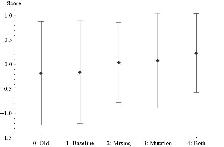
Figure 7: Comparison of normalized rating score distributions between swarms produced under five experimental conditions (from Sayama et al., (2009)). Average rating scores are shown by diamonds, with error bars around them showing standard deviations.

(a)

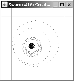
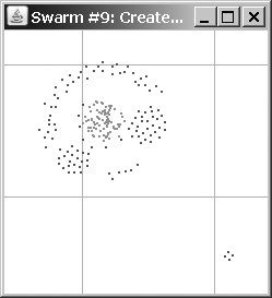
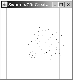
(b)

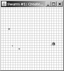
Figure 8: Samples of the final swarm designs created by subjects (from Sayama et al., (2009)). (a) Best three that received the highest rating scores. (b) Worst three that received the lowest rating scores.

To detect statistical differences between experimental conditions, a one-way ANOVA was conducted. The result of the ANOVA is summarized in Table 2. Statistically significant variation was found between the conditions ($p<0.005$). Tukey’s and Bonferroni’s post-hoc tests detected a significant difference between conditions 0 (NIEC) and 4 (HIEC), which supports our hypothesis that the HIEC is more effective at producing final designs of higher quality than NIEC. The post-hoc tests also detected a significant difference between conditions 1 (HIEC without mixing or mutation operators) and 4 (HIEC). These results indicate that the more active role a designer plays in the interactive design process, and the more diverse evolutionary operators she has at her disposal, the more effectively she can guide the evolutionary design of self-organizing swarms.

Table 2: Results of one-way ANOVA on the rating scores for five conditions obtained in experiment 2 (from Bush and Sayama, (2011)). Significant difference is shown with an asterisk.

Source of variation	Degrees of freedom	Sum of squares	Mean square	$F$	$F$-test $p$-value
Between groups	4	14.799	3.700	4.11	0.003*
Within groups	583	525.201	0.901
Total	587	540

4 Automated Approach

The second approach we took was motivated by the following question: Do we really need human users in order to guide designs of self-organizing swarms? This question might sound almost paradoxical, because designing an artifact implies the existence of a designer by definition. However, this argument is quite similar to the “watchmaker” argument claimed by the English theologist William Paley (as well as by many other leading scientists in the past) Dawkins, (1996). Now that we know that the blind evolutionary process did “design” quite complex, intricate structures and functions of biological systems, it is reasonable to assume that it should be possible to create automatic processes that can spontaneously produce various creative self-organizing swarms without any human intervention.

In order to make the swarms capable of spontaneous evolution within a simulated world, we implemented several major modifications to Swarm Chemistry Sayama, (2010, 2011); Sayama and Wong, (2011), as follows:

1. There are now two categories of particles, active (moving and interacting kinetically) and passive (remaining still and inactive). An active particle holds a recipe of the swarm (a list of kinetic parameter sets) (Fig. 9(a)).

2. A recipe is transmitted from an active particle to a passive particle when they collide, making the latter active (Fig. 9(b)).

3. The activated particle differentiates randomly into one of the multiple types specified in the recipe, with probabilities proportional to their ratio in it (Fig. 9(c)).

4. Active particles randomly and independently re-differentiate with small probability, $r$, at every time step ($r=0.005$ for all simulations presented in this chapter).

5. A recipe is transmitted even between two active particles of different types when they collide. The direction of recipe transmission is determined by a competition function that picks one of the two colliding particles as a source (and the other as a target) of transmission based on their properties (Fig. 9(d)).

6. The recipe can mutate when transmitted, as well as spontaneously at every time step, with small probabilities, $p_{t}$ and $p_{s}$, respectively (Fig. 9(e)). In a single recipe mutation event, several mutation operators are applied, including duplication of a kinetic parameter set (5% per set), deletion of a kinetic parameter set (5% per set), addition of a random kinetic parameter set (10% per event; increased to 50% per event in later experiments), and a point mutation of kinetic parameter values (10% per parameter).

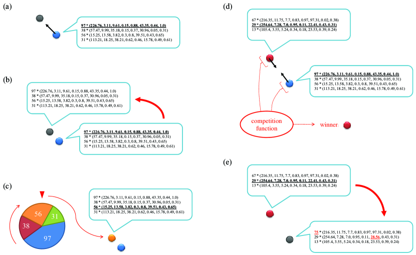
Figure 9: How particle interactions work in the revised Swarm Chemistry (from Sayama, (2011)). (a) There are two categories of particles, active (blue) and passive (gray). An active particle holds a recipe of the swarm in it (shown in the call-out). Each row in the recipe represents one kinetic parameter set. The underline shows which kinetic parameter set the particle is currently using (i.e., which kinetic type it is differentiated into). (b) A recipe is transmitted from an active particle to a passive particle when they collide, making the latter active. (c) The activated particle differentiates randomly into a type specified by one of the kinetic parameter sets in the recipe given to it. (d) A recipe is transmitted between active particles of different types when they collide. The direction of recipe transmission is determined by a competition function that picks one of the two colliding particles as a source (and the other as a target) of transmission based on their properties. (e) The recipe can mutate when transmitted with small probability.

These extensions made the model capable of showing morphogenesis and self-repair Sayama, (2010) and autonomous ecological/evolutionary behaviors of self-organized “super-organisms” made of a number of swarming particles Sayama, (2011); Sayama and Wong, (2011). We note here that there was a technical problem in the original implementation of collision detection in an earlier version of evolutionary Swarm Chemistry Sayama, (2011), which was fixed in the later implementation Sayama and Wong, (2011).

In addition, in order to make evolution occur, we needed to confine the particles in a finite environment in which different recipes compete against each other. We thus conducted all the simulations with 10,000 particles contained in a finite, $5,000\times 5,000$ square space (in arbitrary units; for reference, the maximal perception radius of a particle was 300). A “pseudo”-periodic boundary condition was applied to the boundaries of the space. Namely, particles that cross a boundary reappear from the other side of the space just like in conventional periodic boundary conditions, but they do not interact across boundaries with other particles sitting near the other side of the space. In other words, the periodic boundary condition applies only to particle positions, but not to their interaction forces. This specific choice of boundary treatment was initially made because of its simplicity of implementation, but it proved to be a useful boundary condition that introduces a moderate amount of perturbations to swarms while maintaining their structural coherence and confining them in a finite area.

In the simulations, two different initial conditions were used: a random initial condition made of 9,900 inactive particles and 100 active particles with randomly generated one-type recipes distributed over the space, and a designed initial condition consisted of 9,999 inactive particles distributed over the space, with just one active particle that holds a pre-designed recipe positioned in the center of the space. Specifically, recipes of “swinger”, “rotary” and “walker-follower” (shown in Fig. 4) patterns were used.

4.1 Exploring experimental conditions

Using the evolutionary Swarm Chemistry model described above, we studied what kind of experimental conditions (competition functions and mutation rates) would be most successful in creating self-organizing complex patterns Sayama, (2011).

The first experiment was to observe the basic evolutionary dynamics of the model under low mutation rates ($p_{t}=10^{-3}$, $p_{s}=10^{-5}$). Random and designed (“swinger”) initial conditions were used. The following four basic competition functions were implemented and tested:

• faster: The faster particle wins.

• slower: The slower particle wins.

• behind: The particle that hit the other one from behind wins. Specifically, if a particle exists within a 90-degree angle opposite to the other particle’s velocity, the former particle is considered a winner.

• majority: The particle surrounded by more of the same type wins. The local neighborhood radius used to count the number of particles of the same type was 30. The absolute counts were used for comparison.

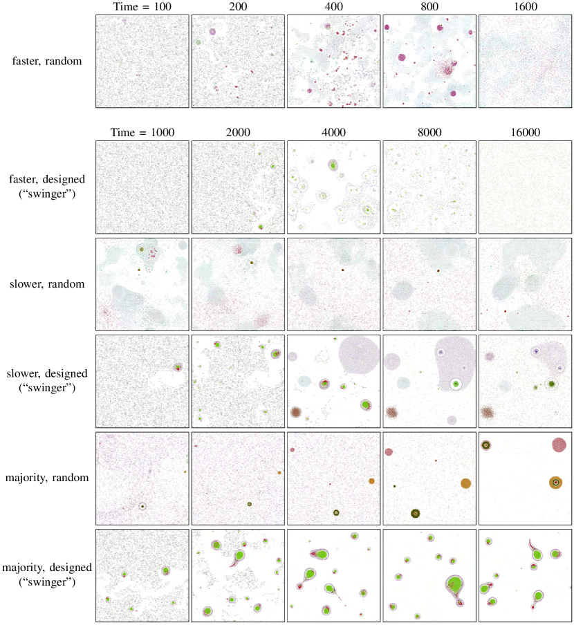
Figure 10: Evolutionary processes observed in the evolutionary Swarm Chemistry model (from Sayama, (2011)). Each image shows a snapshot of the space in a simulation, where dots with different colors represent particles of different types. Labels on the left indicates the competition function and the initial condition used in each case. Snapshots were taken at logarithmic time intervals.

Results are shown in Fig. 10. The results with the “behind” competition function were very similar to those with the “faster” competition function, and therefore omitted from the figure. In general, growth and replication of macroscopic structures were observed at early stages of the simulations. The growth was accomplished by recruitment of inactive particles through collisions. Once a cluster of active particles outgrew maximal size beyond which they could not maintain a single coherent structure (typically determined by their perception range), the cluster spontaneously split into multiple smaller clusters, naturally resulting in the replication of those structures. These growth and replication dynamics were particularly visible in simulations with designed initial conditions. Once formed, the macroscopic structures began to show ecological interactions by themselves, such as chasing, predation and competition over finite resources (i.e., particles), and eventually the whole system tended to settle down in a static or dynamic state where only a small number of species were dominant. There were some evolutionary adaptations also observed (e.g., in faster & designed (“swinger”); second row in Fig. 10) even with the low mutation rates used.

It was also observed that the choice of competition functions had significant impacts on the system’s evolutionary dynamics. Both the “faster” and “behind” competition functions always resulted in an evolutionary convergence to a homogeneous cloud of fast-moving, nearly independent particles. In contrast, the “slower” competition function tended to show very slow evolution, often leading to the emergence of crystallized patterns. The “majority” competition function turned out to be most successful in creating and maintaining dynamic behaviors of macroscopic coherent structures over a long period of time, yet it was quite limited regarding the capability of producing evolutionary innovations. This was because any potentially innovative mutation appearing in a single particle would be lost in the presence of local majority already established around it.

Based on the results of the previous experiment, the following five more competition functions were implemented and tested. The last three functions that took recipe length into account were implemented in the hope that they might promote evolution of increasingly more complex recipes and therefore more complex patterns:

• majority (probabilistic): The particle surrounded by more of the same type wins. This is essentially the same function as the original “majority”, except that the winner is determined probabilistically using the particle counts as relative probabilities of winning.

• majority (relative): The particle that perceives the higher density of the same type within its own perception range wins. The density was calculated by dividing the number of particles of the same type by the total number of particles of any kind, both counted within the perception range. The range may be different and asymmetric between the two colliding particles.

• recipe length: The particle with a recipe that has more kinetic parameter sets wins.

• recipe length then majority: The particle with a recipe that has more kinetic parameter sets wins. If the recipe length is equal between the two colliding particles, the winner is selected based on the “majority” competition function.

• recipe length $\times$ majority: A numerical score is calculated for each particle by multiplying its recipe length by the number of particles of the same type within its local neighborhood (radius = 30). Then the particle with a greater score wins.

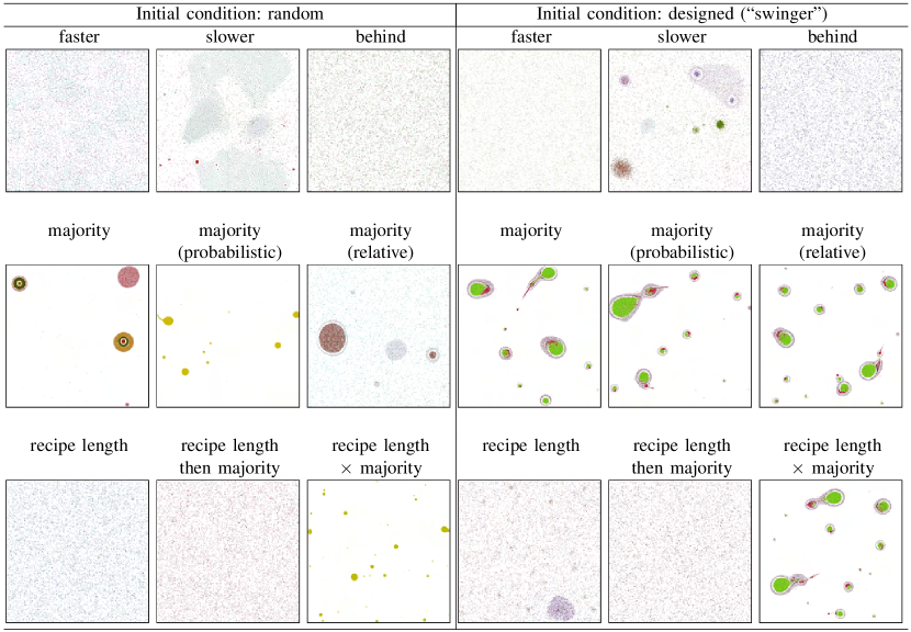
Figure 11: Comparison between several different competition functions (from Sayama, (2011)). The nine cases on the left hand side started with random initial conditions, while the other nine on the right hand side started with designed initial conditions with the “swinger” recipe. Snapshots were taken at time = 20,000 for all cases.

Results are summarized in Fig. 11. As clearly seen in the figure, the majority-based rules are generally good at maintaining macroscopic coherent structures, regardless of minor variations in their implementations. This indicates that interaction between particles, or “cooperation” among particles of the same type to support one another, is the key to creating and maintaining macroscopic structures. Experimental observation of a number of simulation runs gave an impression that the “majority (relative)” competition function would be the best in this regard, therefore this function was used in all of the following experiments.

In the meantime, the “recipe length” and “recipe length then majority” competition functions did not show any evolution toward more complex forms, despite the fact that they would strongly promote evolution of longer recipes. What was occurring in these conditions was an evolutionary accumulation of “garbage” kinetic parameter sets in a recipe, which did not show any interesting macroscopic structure. This is qualitatively similar to the well-known observation made in Tierra Ray, (1992).

The results described above suggested the potential of evolutionary Swarm Chemistry for producing more creative, continuous evolutionary processes, but none of the competition functions showed notable long-term evolutionary changes yet. We therefore increased the mutation rates to a 100 times greater level than those in the experiments above, and also introduced a few different types of exogenous perturbations to create a dynamically changing environment (for more details, see Sayama, (2011)). This was informed by our earlier work on evolutionary cellular automata Salzberg et al., (2004); Salzberg and Sayama, (2004), which demonstrated that such dynamic environments may make evolutionary dynamics of a system more variation-driven and thus promote long-term evolutionary changes.

With these additional changes, some simulation runs finally demonstrated continuous changes of dominant macroscopic structures over a long period of time (Fig. 12). A fundamental difference between this and earlier experiments was that the perturbation introduced to the environment would often break the “status quo” established in the swarm population, making room for further evolutionary innovations to take place. A number of unexpected, creative swarm designs spontaneously emerged out of these simulation runs, fulfilling our intension to create automated evolutionary design processes. Videos of sample simulation runs can be found on our YouTube channel (http://youtube.com/ComplexSystem).

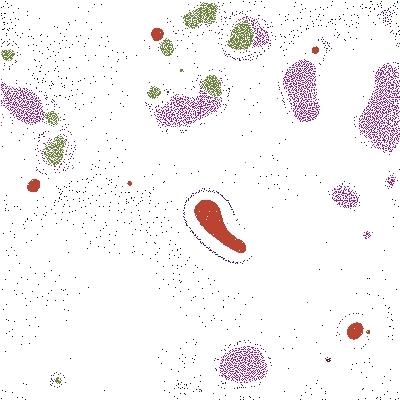
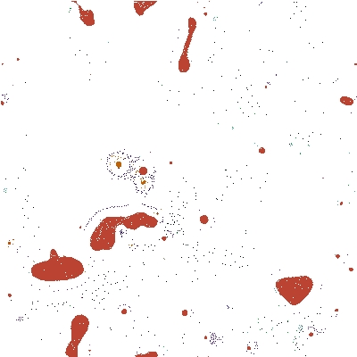
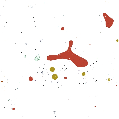
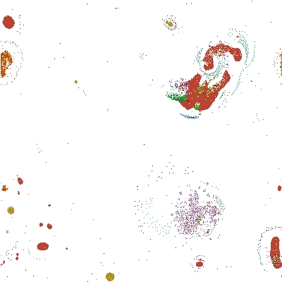
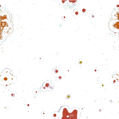
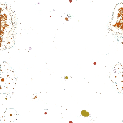
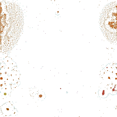
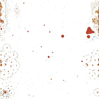
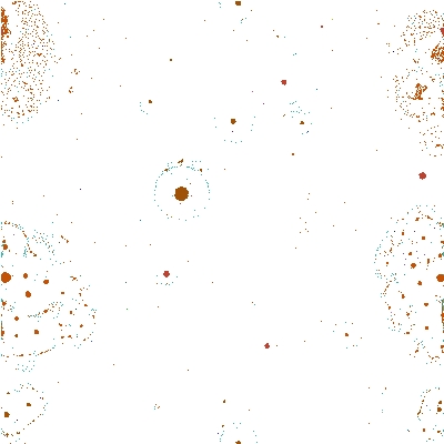
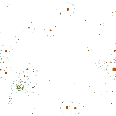
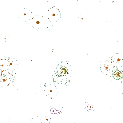
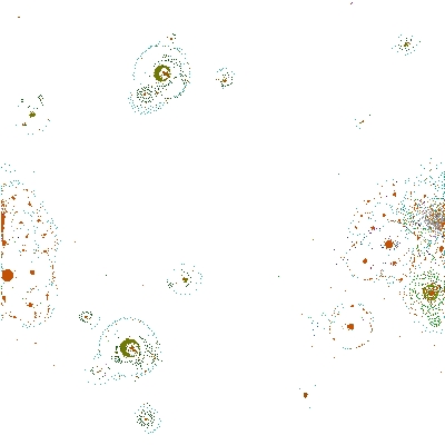
Figure 12: An example of long-term evolutionary behavior seen under dynamic environmental conditions with high mutation rates. Snapshots were taken at constant time intervals (2,500 steps) to show continuous evolutionary changes.

4.2 Quantifying observed evolutionary dynamics

The experimental results described above were quite promising, but they were evaluated only by visual inspection with no objective measurements involved. To address the lack of quantitative measurements, we developed and tested two simple measurements to quantify the degrees of evolutionary exploration and macroscopic structuredness of swarm populations Sayama and Wong, (2011), assuming that the evolutionary process of swarms would look interesting and creative to human eyes if it displayed patterns that are clearly visible and continuously changing. These measurements were developed so that they can be easily calculated a posteriori from a sequence of snapshots (bitmap images) taken in past simulation runs, without requiring genotypic or genealogical information that was typically assumed available in other proposed metrics Bedau and Packard, (1992); Bedau and Brown, (1999); Nehaniv, (2000).

Evolutionary exploration was quantified by counting the number of new RGB colors that appeared in a bitmap image of the simulation snapshot at a specific time point for the first time during each simulation run (Fig. 13, right). Since different particle types are visualized with different colors in Swarm Chemistry, this measurement roughly represents how many new particle types emerged during the last time segment. Macroscopic structuredness was quantified by measuring a Kullback-Leibler divergence Kullback and Leibler, (1951) of a pairwise particle distance distribution from that of a theoretical case where particles are randomly and homogeneously spread over the entire space (Fig. 13, left). Specifically, each snapshot bitmap image was first analyzed and converted into a list of coordinates (each representing the position of a particle, or a colored pixel), then a pair of coordinates were randomly sampled from the list 100,000 times to generate an approximate pairwise particle distance distribution in the bitmap image. The Kullback-Leibler divergence of the approximate distance distribution from the homogeneous case is larger when the swarm is distributed in a less homogeneous manner, forming macroscopic structures.

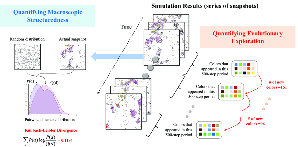
Figure 13: Methods to quantify evolutionary exploration (right) and macroscopic structuredness (left) directly from a sequence of snapshots (bitmap images, center).

Table 3: Four conditions used for the final experiment to quantify evolutionary dynamics.

Name	Mutation rate	Environmental	Collision detection
		perturbation	algorithm
original-low	low	off	original
original-high	high	on	original
revised-low	low	off	revised
revised-high	high	on	revised

We applied these measurements to simulation runs obtained under each of the four conditions shown in Table 3. Results are summarized in Figs. 14 and 15. Figure 14 clearly shows the high evolutionary exploration occurring under the conditions with high mutation rates and environmental perturbations. In the meantime, Figure 15 shows that the “original-high” condition had a tendency to destroy macroscopic structures by allowing swarms to evolve toward simpler, homogeneous forms. Such degradation of structuredness over time was, as mentioned earlier, due to a technical problem in the previous implementation of collision detection Sayama, (2011); Sayama and Wong, (2011) that mistakenly depended on perception ranges of particles. The “revised” conditions used a fixed collision detection algorithm. This modification was found to have an effect to maintain macroscopic structures for a prolonged period of time (Fig. 15). Combining these results together (Fig. 16), we were able to detect automatically that the “revised-high” condition was most successful in producing interesting designs, maintaining macroscopic structures without losing evolutionary exploration. This conclusion also matched subjective observations made by human users.

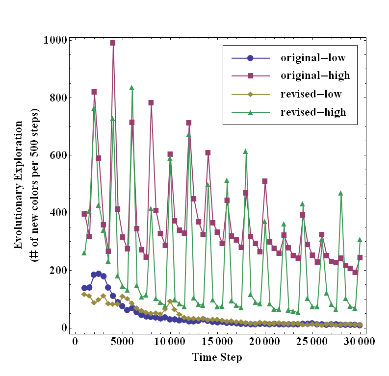
Figure 14: Temporal changes of the evolutionary exploration measurement (i.e., number of new colors per 500 time steps) for four different experimental conditions, calculated from snapshots of simulation runs taken at 500 time step intervals (from Sayama and Wong, (2011)). Each curve shows the average result over 12 simulation runs (3 independent runs $\times$ 4 different initial conditions given in Sayama, (2011)). Sharp spikes seen in “high” conditions were due to dynamic exogenous perturbations.

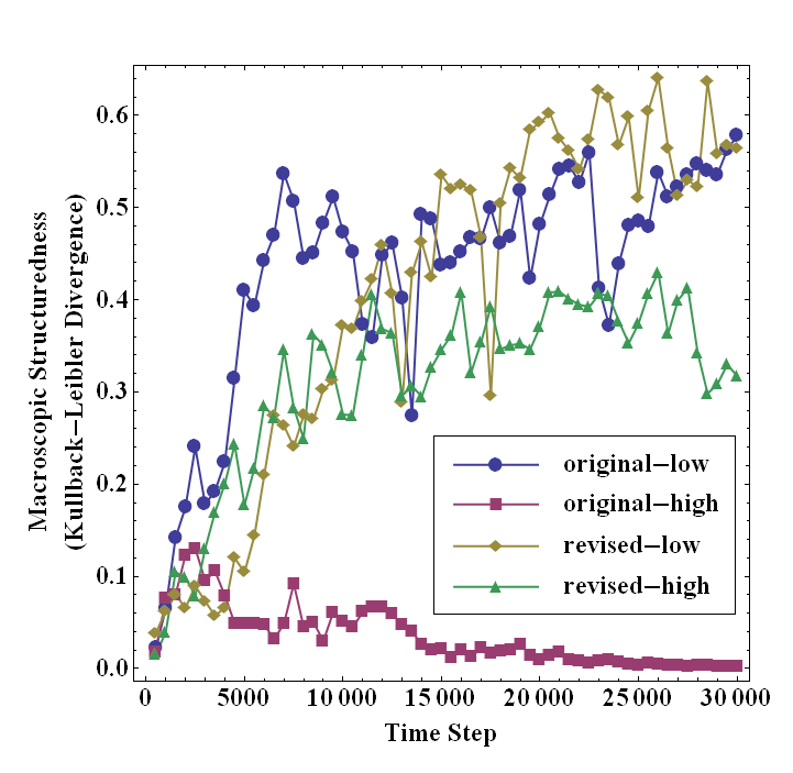
Figure 15: Temporal changes of the macroscopic structuredness measurement (i.e., Kullback-Leibler divergence of the pairwise particle distance distribution from that of a purely random case) for four different experimental conditions, calculated from snapshots of simulation runs taken at 500 time step intervals (from Sayama and Wong, (2011)). Each curve shows the average result over 12 simulation runs (3 independent runs   4 different initial conditions). The “original-high” condition loses macroscopic structures while other conditions successfully maintain them.

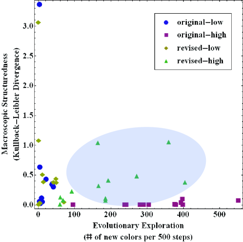
Figure 16: Evolutionary exploration and macroscopic structuredness averaged over $t=10,000-30,000$ for each independent simulation run (from Sayama and Wong, (2011), with slight modifications). Each marker represents a data point taken from a single simulation run. It is clearly observed that the “revised-high” condition (shaded in light blue) most successfully achieved high evolutionary exploration without losing macroscopic structuredness.

5 Conclusions

In this chapter, we have reviewed our recent work on two complementary approaches for guiding designs of self-organizing heterogeneous swarms. The common design challenge addressed in both approaches was the lack of explicit criteria for what constitutes a “good” design to produce. In the first approach, this challenge was solved by having a human user as an active initiator of evolutionary design processes. In the second approach, the criteria were replaced by low-level competition functions (similar to laws of physics) that drive spontaneous evolution of swarms in a virtual ecosystem.

The core message arising from both approaches is the unique power of evolutionary processes for designing self-organizing complex systems. It is uniquely powerful because evolution does not require any macroscopic plan, strategy or global direction for the design to proceed. As long as the designer—this could be either an intelligent entity or a simple unintelligent machinery—can make local decisions at microscopic levels, the process drives itself to various novel designs through unprescribed evolutionary pathways. Designs made through such open-ended evolutionary processes may have a potential to be more creative and innovative than those produced through optimization for explicit selection criteria.

We conclude this chapter with a famous quote by Richard Feynman. At the time of his death, Feynman wrote on a blackboard, “What I cannot create, I do not understand.” This is a concise yet profound sentence that beautifully summarizes the role and importance of constructive understanding (i.e., model building) in scientific endeavors, which hits home particularly well for complex systems researchers. But research on evolutionary design of complex systems, including ours discussed here, has illustrated that the logical converse of the above quote is not necessarily true. That is, evolutionary approaches make this also possible—“What I do not understand, I can still create.”

References

- Anderson, (2006) Anderson, C. (2006). Creation of desirable complexity: strategies for designing selforganized systems. In Complex Engineered Systems, pages 101–121. Springer.
- Banzhaf, (2000) Banzhaf, W. (2000). Interactive evolution. Evolutionary Computation, 1:228–236.
- Bar-Yam, (2003) Bar-Yam, Y. (2003). Dynamics of complex systems. Westview Press.
- Bedau and Brown, (1999) Bedau, M. A. and Brown, C. T. (1999). Visualizing evolutionary activity of genotypes. Artificial Life, 5(1):17–35.
- Bedau and Packard, (1992) Bedau, M. A. and Packard, N. H. (1992). Measurement of evolutionary activity, teleology, and life. In Artificial Life II, pages 431–461. Addison-Wesley.
- Bentley, (1999) Bentley, P. (1999). Evolutionary design by computers. Morgan Kaufmann.
- Bentley and O’Reilly, (2001) Bentley, P. J. and O’Reilly, U.-M. (2001). Ten steps to make a perfect creative evolutionary design system. In GECCO 2001 Workshop on Non-Routine Design with Evolutionary Systems.
- Boccara, (2010) Boccara, N. (2010). Modeling complex systems. Springer.
- Bush and Sayama, (2011) Bush, B. J. and Sayama, H. (2011). Hyperinteractive evolutionary computation. Evolutionary Computation, IEEE Transactions on, 15(3):424–433.
- Camazine, (2003) Camazine, S. (2003). Self-organization in biological systems. Princeton University Press.
- Cheng et al., (2005) Cheng, J., Cheng, W., and Nagpal, R. (2005). Robust and self-repairing formation control for swarms of mobile agents. In AAAI, volume 5, pages 59–64.
- Couzin et al., (2002) Couzin, I. D., Krause, J., James, R., Ruxton, G. D., and Franks, N. R. (2002). Collective memory and spatial sorting in animal groups. Journal of theoretical biology, 218(1):1–11.
- Dawkins, (1996) Dawkins, R. (1996). The blind watchmaker: Why the evidence of evolution reveals a universe without design. WW Norton & Company.
- Dittrich et al., (2001) Dittrich, P., Ziegler, J., and Banzhaf, W. (2001). Artificial chemistries \areview. Artificial life, 7(3):225–275.
- Doursat et al., (2012) Doursat, R., Sayama, H., and Michel, O. (2012). Morphogenetic engineering: Reconciling self-organization and architecture. In Morphogenetic Engineering, pages 1–24. Springer.
- Hemelrijk and Kunz, (2005) Hemelrijk, C. K. and Kunz, H. (2005). Density distribution and size sorting in fish schools: an individual-based model. Behavioral Ecology, 16(1):178–187.
- Kullback and Leibler, (1951) Kullback, S. and Leibler, R. A. (1951). On information and sufficiency. The Annals of Mathematical Statistics, 22(1):79–86.
- Kunz and Hemelrijk, (2003) Kunz, H. and Hemelrijk, C. K. (2003). Artificial fish schools: collective effects of school size, body size, and body form. Artificial life, 9(3):237–253.
- Minai et al., (2006) Minai, A. A., Braha, D., and Bar-Yam, Y. (2006). Complex engineered systems: A new paradigm. Springer.
- Nehaniv, (2000) Nehaniv, C. L. (2000). Measuring evolvability as the rate of complexity increase. In Artificial Life VII Workshop Proceedings, pages 55–57.
- Newman and Sayama, (2008) Newman, J. P. and Sayama, H. (2008). Effect of sensory blind zones on milling behavior in a dynamic self-propelled particle model. Physical Review E, 78(1):011913.
- Ottino, (2004) Ottino, J. M. (2004). Engineering complex systems. Nature, 427(6973):399–399.
- Pahl et al., (2007) Pahl, G., Wallace, K., and Blessing, L. (2007). Engineering design: a systematic approach, volume 157. Springer.
- Ray, (1992) Ray, T. S. (1992). An approach to the synthesis of life. In Artificial Life II, pages 371–408. Addison-Wesley.
- Reynolds, (1987) Reynolds, C. W. (1987). Flocks, herds and schools: A distributed behavioral model. ACM SIGGRAPH Computer Graphics, 21(4):25–34.
- Salzberg et al., (2004) Salzberg, C., Antony, A., and Sayama, H. (2004). Evolutionary dynamics of cellular automata-based self-replicators in hostile environments. BioSystems, 78(1):119–134.
- Salzberg and Sayama, (2004) Salzberg, C. and Sayama, H. (2004). Complex genetic evolution of artificial self-replicators in cellular automata. Complexity, 10(2):33–39.
- Sayama, (2007) Sayama, H. (2007). Decentralized control and interactive design methods for large-scale heterogeneous self-organizing swarms. In Advances in Artificial Life, pages 675–684. Springer.
- Sayama, (2009) Sayama, H. (2009). Swarm chemistry. Artificial Life, 15(1):105–114.
- Sayama, (2010) Sayama, H. (2010). Robust morphogenesis of robotic swarms. Computational Intelligence Magazine, IEEE, 5(3):43–49.
- Sayama, (2011) Sayama, H. (2011). Seeking open-ended evolution in swarm chemistry. In Artificial Life (ALIFE), 2011 IEEE Symposium on, pages 186–193. IEEE.
- Sayama, (2012) Sayama, H. (2012). Swarm-based morphogenetic artificial life. In Morphogenetic Engineering, pages 191–208. Springer.
- Sayama et al., (2009) Sayama, H., Dionne, S., Laramee, C., and Wilson, D. S. (2009). Enhancing the architecture of interactive evolutionary design for exploring heterogeneous particle swarm dynamics: An in-class experiment. In Artificial Life, 2009. ALife’09. IEEE Symposium on, pages 85–91. IEEE.
- Sayama and Wong, (2011) Sayama, H. and Wong, C. (2011). Quantifying evolutionary dynamics of swarm chemistry. In Advances in Artificial Life, ECAL 2011: Proceedings of the Eleventh European Conference on Artificial Life, pages 729–730.
- Shneiderman et al., (2009) Shneiderman, B., Plaisant, C., Cohen, M., and Jacobs, S. (2009). Designing the User Interface: Strategies for Effective Human-Computer Interaction (5th Edition). Prentice Hall.
- Sole and Goodwin, (2008) Sole, R. and Goodwin, B. (2008). Signs of life: How complexity pervades biology. Basic books.
- Takagi, (2001) Takagi, H. (2001). Interactive evolutionary computation: Fusion of the capabilities of ec optimization and human evaluation. Proceedings of the IEEE, 89(9):1275–1296.
- Unemi, (2003) Unemi, T. (2003). Simulated breeding–a framework of breeding artifacts on the computer. Kybernetes, 32(1/2):203–220.