\includeversion

GraphsAsImages \excludeversionGraphsAsMatrices

Axioms for graph clustering quality functions

\nameTwan van Laarhoven \emailtvanlaarhoven@cs.ru.nl \AND\nameElena Marchiori \emailelenam@cs.ru.nl
\addrInstitute for Computing and Information Sciences
Radboud University Nijmegen
Postbus 9010
6500 GL Nijmegen, The Netherlands
Abstract

We investigate properties that intuitively ought to be satisfied by graph clustering quality functions, i.e. functions that assign a score to a clustering of a graph. Graph clustering, also known as network community detection, is often performed by optimizing such a function. Two axioms tailored for graph clustering quality functions are introduced, and the four axioms introduced in previous work on distance based clustering are reformulated and generalized for the graph setting. We show that modularity, a standard quality function for graph clustering, does not satisfy all of these six properties. This motivates the derivation of a new family of quality functions, adaptive scale modularity, which does satisfy the proposed axioms. Adaptive scale modularity has two parameters, which give greater flexibility in the kinds of clusterings that can be found. Standard graph clustering quality functions, such as normalized cut and unnormalized cut, are obtained as special cases of adaptive scale modularity.

In general, the results of our investigation indicate that the considered axiomatic framework covers existing ‘good’ quality functions for graph clustering, and can be used to derive an interesting new family of quality functions.

Keywords: graph clustering, modularity, axiomatic framework.

1 Introduction

Following the work by Kleinberg (2002) there have been various contributions to the theoretical foundation and analysis of clustering, such as axiomatic frameworks for quality functions (Ackerman and Ben-David, 2008), for criteria to compare clusterings (Meila, 2005), uniqueness theorems for specific types of clustering (Zadeh and Ben-David, 2009; Ackerman and Ben-David, 2013; Carlsson, Mémoli, Ribeiro, and Segarra, 2013), taxonomy of clustering paradigms (Ackerman et al., 2010a), and characterization of diversification systems (Gollapudi and Sharma, 2009).

Kleinberg focused on clustering functions, which are functions from a distance function to a clustering. He showed that there are no clustering functions that simultaneously satisfy three intuitive properties: scale invariance, consistency and richness. Ackerman and Ben-David (2008) continued on this work, and showed that the impossibility result does not apply when formulating these properties in terms of quality functions instead of clustering functions, where consistency is replaced with a weaker property called monotonicity.

Both of these previous works are formulated in terms of distance functions over a fixed domain. In this paper we focus on weighted graphs, where the weight of an edge indicates the strength of a connection. The clustering problem on graphs is also known as network community detection.

Graphs provide additional freedoms over distance functions. In particular, it is possible for two points to be unrelated, indicated by a weight of 00. These zero-weight edges in turn make it natural to consider graphs over different sets of nodes as part of a larger graph. Secondly, we can allow for self loops. Self loops can indicate internal edges in a node. This notation is used for instance by Blondel et al. (2008), where a graph is contracted based on a fine-grained clustering.

In this setting, where edges with weight 00 are possible, Kleinberg’s impossibility result does not apply. This can be seen by considering the connected components of a graph. This is a graph clustering function that satisfies all three of Kleinberg’s axioms: scale invariance, consistency and richness (see Section 4.2).

Our focus is on the investigation of graph clustering quality functions, which are functions from a graph and a clustering to a real number ‘quality’. A notable example is modularity (Newman and Girvan, 2004). In particular we ask which properties of quality functions intuitively ought to hold, and which are often assumed to hold when reasoning informally about graph clustering. Such properties might be called axioms for graph clustering.

The rest of this paper is organized as follows: Section 2 gives basic definitions. Next, section 3 discusses different ways in which properties could be formulated.

In Section 4 of this paper we propose an axiomatic framework that consists of six properties of graph clustering quality functions: the (adaption of) the four axioms from Kleinberg (2002) and Ackerman and Ben-David (2008) (permutation invariance, scale invariance, richness and monotonicity); and two additional properties specific for the graph setting (continuity and the locality).

Then, in Section 5, we show that modularity does not satisfy the monotonicity and locality properties.

This result motivates the analysis of variants of modularity, leading to the derivation of a new parametric quality function in Section 6, that satisfies all properties. This quality function, which we call adaptive scale modularity, has two parameters, $M$ and $\gamma$ which can be tuned to control the resolution of the clustering. We show that quality functions similar to normalized cut and unnormalized cut are obtained in the limit when $M$ goes to zero and to infinity, respectively. Furthermore, setting $\gamma$ to 00 yields a parametric quality function similar to that proposed by Reichardt and Bornholdt (2004).

1.1 Related Work

Previous axiomatic studies of clustering quality functions have focused mainly on hierarchical clustering and on weakest and strongest link style quality functions (Kleinberg, 2002; Ackerman and Ben-David, 2008; Zadeh and Ben-David, 2009; Carlsson et al., 2013). Papers in this line of work that focussed also on the partitional setting include Puzicha et al. (1999); Ackerman et al. (2012, 2013). Puzicha et al. (1999) investigated a particular class of clustering quality functions obtained by requiring the function to decompose into a certain additive form. Ackerman et al. (2012) considered clustering in the weighted setting, in which every data point is assigned a real valued weight. They performed a theoretical analysis on the influence of weighted data on standard clustering algorithms. Ackerman et al. (2013) analyzed robustness of clustering algorithms to the addition of a small set of points, and investigated the robustness of popular clustering methods.

All these studies are framed in terms of distance (or similarity and dissimilarity) functions.

Bubeck and Luxburg (2009) studied statistical consistency of clustering methods. They introduced the so-called nearest neighbor clustering and showed its consistency also for standard graph based quality functions, such as normalized cut, ratio cut, and modularity. Here we do not focus on properties of methods to optimize clustering quality, but on natural properties that quality functions for graph clustering should satisfy.

Related works on graph clustering quality functions mainly focus on the so-called resolution limit, that is, the tendency of a quality function to prefer either small or large clusters. In particular, Fortunato and Barthélemy (2007) proved that modularity may not detect clusters smaller than a scale which depends on the total size of the network and on the degree of interconnectedness of the clusters. van Laarhoven and Marchiori (2013) showed that the resolution limit is the most important difference between quality functions in graph clustering optimized using local search optimization.

To mitigate the resolution limit phenomenon, the quality function may be extended with a so-called resolution parameter. For example, Reichardt and Bornholdt (2006) proposed a formulation of graph clustering (therein called network community detection) based on principles from statistical mechanics. This interpretation leads to the introduction of a family of quality functions with a parameter that allows to control the clustering resolution. In Section 6.1 we will show that this extension is a special case of adaptive scale modularity.

Traag, Van Dooren, and Nesterov (2011) formalized the notion of resolution-free quality functions, that is, not suffering from the resolution limit, and provided a characterization of this class of quality functions. Their notion is essentially an axiom, and we will discuss the relation to our axioms in Section 4.1.1.

2 Definitions and Notation

A symmetric weighted graph is a pair $(V,E)$ of a finite set $V$ of nodes and a function $E:V\times V\to\mathbb{R}_{\geq 0}$ of edge weights, where $E(i,j)=E(j,i)$ for all $i,j\in V$. Edges with larger weights represent stronger connections, so missing edges can get weight 00. Note that this is the opposite of the convention used in distance based clustering. We explicitly allow for self loops, that is, nodes for which $E(i,i)>0$.

A clustering $C$ of a graph $G=(V,E)$ is a partition of its nodes. That is, $\bigcup C=V$ and for all $c_{1},c_{2}\in C$, $c_{1}\cap c_{2}\neq\emptyset$ if and only if $c_{1}=c_{2}$. When two nodes $i$ and $j$ are in the same cluster in clustering $C$, i.e. when $i,j\in c$ for some $c\in C$, then we write $i\sim_{C}j$. Otherwise we write $i\not\sim_{C}j$.

A clustering $C$ is a refinement of a clustering $D$, written $C\sqsubseteq D$, when for every cluster $c\in C$ there is a cluster $d\in D$ such that $c\subseteq d$.

A graph clustering quality function (or objective function) $Q$ is a function from graphs $G$ and clusterings of $G$ to real numbers. We adopt the convention that a higher quality indicates a ‘better’ clustering. As a generalization, we will sometimes work with parameterized families of quality functions. A single quality function can be seen as a family with no parameters.

Let $G_{1}=(V_{1},E_{1})$ and $G_{2}=(V_{2},E_{2})$ be two graphs and let $V_{a}\subseteq V_{1}\cap V_{2}$ be a subset of the common nodes. We say that the graphs agree on $V_{a}$ if $E_{1}(i,j)=E_{2}(i,j)$ for all $i,j\in V_{a}$. We say that the graphs also agree on the neighborhood of $V_{a}$ If

  • $E_{1}(i,j)=E_{2}(i,j)$ for all $i\in V_{a}$ and $j\in V_{1}\cap V_{2}$,

  • $E_{1}(i,j)=0$ for all $i\in V_{a}$ and $j\in V_{1}\setminus V_{2}$, and

  • $E_{2}(i,j)=0$ for all $i\in V_{a}$ and $j\in V_{2}\setminus V_{1}$.

This means that for nodes in $V_{a}$ the weights and endpoints of incident edges are exactly the same in the two graphs.

3 On the Form of Axioms

There are three different ways to state potential axioms for clustering:

  1. 1.

    As a property of clustering functions, as in Kleinberg (2002). For example, scale invariance of a clustering function $\hat{C}$ would be written as “$\hat{C}(G)=\hat{C}(\alpha G)$, for all graphs $G$, $\alpha>0$”. I.e. the optimal clustering is invariant under scaling of edge weights.

  2. 2.

    As a property of the values of a quality function $Q$, as in Ackerman and Ben-David (2008). For example “$Q(G,C)=Q(\alpha G,C)$, for all graphs $G$, all clustering $C$ of $G$, and $\alpha>0$”. I.e. the quality is invariant under scaling of edge weights.

  3. 3.

    As a property of the relation between qualities of different clustering, or equivalently, as a property of an ordering of clusterings for a particular graph. For example “$Q(G,C)\geq Q(G,D)\Rightarrow Q(\alpha G,C)\geq Q(\alpha G,D)$”.I.e. the ‘better than’ relation for clusterings is invariant under scaling of edge weights.

The third form is slightly more flexible than the other two. Any quality function that satisfies a property in the second style will also satisfy the corresponding property in the third style, but the converse is not true. Note also that if $D$ is not restricted in a property in the third style, then one can take $\hat{C}(G)=\operatorname{argmax}_{C}Q(G,C)$ to obtain a clustering function and an axiom in the first style.

Most properties are more easily stated and proved in the second, absolute, style. Therefore, we adopt the second style unless doing so requires us to make specific choices.

4 Axioms for Graph Clustering Quality Functions

Kleinberg defined three axioms for distance based clustering functions. In Ackerman and Ben-David (2008) the authors reformulated these into four axioms for clustering quality functions. These axioms can easily be adapted to the graph setting.

The first property that one expects for graph clustering is that the quality of a clustering depends only on the graph, that is, only on the weight of edges between nodes, not on the identity of nodes. We formalize this in the permutation invariance axiom,

Definition 1 (Permutation invariance)

A graph clustering quality function $Q$ is permutation invariant if for all graphs $G=(V,E)$ and all isomorphisms $f:V\to V^{\prime}$, it is the case that $Q(G,C)=Q(f(G),f(C))$; where $f$ is extended to graphs and clusterings by $f(C)=\{\{f(i)\mid i\in c\}\mid c\in C\}$ and $f((V,E))=(V^{\prime},(i,j)\mapsto E(f^{-1}(i),f^{-1}(j)))$.

The second property, scale invariance, requires that the quality doesn’t change when edge weights are scaled uniformly. This is an intuitive axiom when one thinks in terms of units: a graph with edges in “m/s” can be scaled to a graph with edges in “km/h”. The quality should not be affected by such a transformation, perhaps up to a change in units.

Ackerman and Ben-David (2008) defined scale invariance by insisting that the quality stays equal when distances are scaled. In contrast, in Puzicha et al. (1999) the quality should scale proportional with the scaling of distances. We generalize both of these previous definitions by only considering the relations between the quality of two clusterings.

Definition 2 (Scale invariance)

A graph clustering quality function $Q$ is scale invariant if for all graphs $G=(V,E)$, all clusterings $C_{1},C_{2}$ of $G$ and all constants $\alpha>0$, $Q(G,C_{1})\leq Q(G,C_{2})$ if and only if $Q(\alpha G,C_{1})\leq Q(\alpha G,C_{2})$. Where $\alpha G=(V,(i,j)\mapsto\alpha E(i,j))$ is a graph with edge weights scaled by a factor $\alpha$.

This formulation is flexible enough for single quality functions. However, families of quality functions could have parameters that are also scale dependent. For such families we therefore propose to use as an axiom a more flexible property that also allows the parameters to be scaled,

Definition 3 (Scale invariant family)

A family of quality function $Q_{P}$ parameterized by $P\in\mathcal{P}$ is scale invariant if for all constants $P\in\mathcal{P}$ and $\alpha>0$ there is a $P^{\prime}\in\mathcal{P}$ such that for all graphs $G=(V,E)$, and all clusterings $C_{1},C_{2}$ of $G$, $Q_{P}(G,C_{1})\leq Q_{P}(G,C_{2})$ if and only if $Q_{P^{\prime}}(\alpha G,C_{1})\leq Q_{P^{\prime}}(\alpha G,C_{2})$.

Thirdly, we want to rule out trivial quality functions. This is done by requiring richness, i.e. that by changing the edge weights any clustering can be made optimal for that quality function.

Definition 4 (Richness)

A graph clustering quality function $Q$ is rich if for all sets $V$ and all non-trivial partitions $C^{*}$ of $V$, there is a graph $G=(V,E)$ such that $C^{*}$ is the $Q$-optimal clustering of $V$, i.e. $\operatorname{argmax}_{C}Q(G,C)=C^{*}$.

The last axiom that Ackerman and Ben-David consider is by far the most interesting. Intuitively, we expect that when the edges within a cluster are strengthened, or when edges between clusters are weakened, that this does not decrease the quality. Formally we call such a change of a graph a consistent improvement,

Definition 4 (Consistent improvement)

Let $G=(V,E)$ be a graph and $C$ a clustering of $G$. A graph $G^{\prime}=(V,E^{\prime})$ is a $C$-consistent improvement of $G$ if for all nodes $i$ and $j$, $E^{\prime}(i,j)\geq E(i,j)$ whenever $i\sim_{C}j$ and $E^{\prime}(i,j)\leq E(i,j)$ whenever $i\not\sim_{C}j$.

We say that a quality function that does not decrease under consistent improvement is monotonic. In previous work this axiom is often called consistency.

Definition 5 (Monotonicity)

A graph clustering quality function $Q$ is monotonic if for all graphs $G$, all clusterings $C$ of $G$ and all $C$-consistent improvements $G^{\prime}$ of $G$ it is the case that $Q(G^{\prime},C)\geq Q(G,C)$.

4.1 Locality

In the graph setting it also becomes natural to look at combining different graphs. With distance functions this is impossible, since it is not clear what the distance between nodes from the two different sets should be. But for graphs we can take the edge weight between nodes not in both graphs to be zero, which is the case when the graphs agree on the neighborhood of some set.

Consider adding nodes to one side of a large network, then we would not want the clustering on the other side of the network to change if there is no direct connection. For example, if a new protein is discovered in yeast, then the clustering of unrelated proteins in humans should remain the same. Similarly, we can consider any two graphs with disjoint node sets as one larger graph. Then the quality of clusterings of the two original graphs should relate directly to quality on the combined graph.

In general, local changes to a graph should have only local consequences to a clustering. Or in other words, the contribution of a single cluster to the total quality should only depend on nodes in the neighborhood of that cluster.

Definition 6 (Locality)

A graph clustering quality function $Q$ is local if for all graphs $G_{1}=(V_{1},E_{1})$ and $G_{2}=(V_{2},E_{2})$ that agree on a set $V_{a}$ and its neighborhood, and for all clusterings $C_{a},D_{a}$ of $V_{a}$, $C_{1}$ of $V_{1}\setminus V_{a}$ and $C_{2}$ of $V_{2}\setminus V_{a}$, if $Q(G_{1},C_{a}\cup C_{1})\geq Q(G_{1},D_{a}\cup C_{1})$ then $Q(G_{2},C_{a}\cup C_{2})\geq Q(G_{2},D_{a}\cup C_{2})$.

Any quality function that has a preference for a fixed number of clusters will not be local. On the other hand, a quality function that is written as a sum over clusters, where each summand depends only on properties of nodes and edges in one cluster and not on global properties, is local.

Ackerman et al. (2010b) defined a similar locality property for clustering functions. Their definition differs from ours in three ways. First of all, they looked at $k$-clustering, where the number of clusters is given and fixed. Secondly, their locality property only implies a consistent clustering when the rest of the graph is removed, corresponding to $V_{2}=V_{1}\cap V_{a}$. They do not consider the other direction, where more nodes and edges are added. Finally, their locality property requires only agreement of the overlapping set $V_{a}$, not on its neighborhood. That means that clustering functions should also give the same results if edges with one endpoint in $V_{a}$ are removed.

4.1.1 Relation to Resolution-Limit-Free Quality Functions

Traag et al. (2011) introduced the notion of resolution-limit-free quality functions, which is similar to locality. They then showed that resolution-limit-free quality functions do not suffer from the resolution limit as described by Fortunato and Barthélemy (2007). Their definition is as follows.

Definition 6 (Resolution-limit-free)

Call a clustering $C$ of a graph $G$ $Q$-optimal if for all clustering $C^{\prime}$ of $G$ we have that $Q(G,C)\geq Q(G,C^{\prime})$. Let $C$ be a $Q$-optimal clustering of a graph $G_{1}$. Then the quality function $Q$ is called resolution-limit-free if for each subgraph $G_{2}$ induced by $D\subset C$, the partition $D$ is also $Q$-optimal.

There are three differences compared to our locality property. First of all, Definition 2 refers only to the optimal clustering, not to the quality, i.e. it is a property in the style of Kleinberg. Secondly, locality does not require that $G_{2}$ be a subgraph of $G_{1}$. Locality is stronger in that sense. Thirdly, and perhaps most importantly, in the subgraph $G_{2}$ induced by $D\subset C$, edges from a node in $D$ to nodes not in $D$ will be removed. That means that while $G_{1}$ and $G_{2}$ agree on the set of common nodes, they do not also agree on their neighborhood. So in this sense locality is weaker than resolution-limit-freedom.

The notion of resolution-limit-free quality functions was born out of the need to avoid the resolution limit of graph clustering. And indeed locality is not enough to guarantee that a quality function is free from this resolution limit.

We could look at a stronger version of locality, which replaces agreement on the neighborhood of a set $V_{a}$ by plain agreement on that set. Such a strong locality property would imply resolution-limit-freedom. However, it is a very strong property in that it rules out many sensible quality functions. In particular, a strongly local quality function can not depend on the weight of edges entering or leaving a cluster, because that weight can be different in another graph that agrees only on that cluster.

The solution used by Traag et al. is to use the number of nodes instead of the volume of a cluster. In this way they obtain a resolution-limit-free variant of the Potts model by Reichardt and Bornholdt (2004), which they call the constant Potts model. But this comes at the cost of scale invariance.

4.2 Continuity

In the context of graphs, perhaps the most intuitive clustering function is finding the connected components of a graph. As a quality function, we could write

$$Q_{\text{coco}}(G,C)=\mathbf{1}[C=\hat{C}_{\text{coco}}(G)],$$

where the function $\hat{C}_{\text{coco}}$ yields the connected components of a graph.

This quality function is clearly permutation invariant, scale invariant, rich, and local. Since a consistent change can only remove edges between clusters and add edges within clusters, the coco quality function is also monotonic.

In fact, all of Kleinberg’s axioms (reformulated in terms of graphs) also hold for $\hat{C}_{\text{coco}}$, which seems to refute their impossibility result. However, the impossibility proof can not be directly transfered to graphs, because it involves a multiplication and division by a maximum distance. In the graph setting this would be multiplication and division by a minimum edge weight, which can be zero.

Still, despite connected components satisfying all previously defined properties (except for strong locality), it is not a very useful quality function. In many real-world graphs, most nodes are part of one giant connected component (Bollobás, 2001). We would also like the clustering to be influenced by the weight of edges, not just by their existence. A natural way to rule out such degenerate quality functions is to require continuity.

Definition 7 (Continuity)

A quality function $Q$ is continuous if a small change in the graph leads to a small change in the quality. Formally, $Q$ is continuous if for every $\epsilon>0$ and every graph $G=(V,E)$ there exists a $\delta>0$ such that for all graphs $G^{\prime}=(V,E^{\prime})$, if $E(i,j)-\delta<E^{\prime}(i,j)<E(i,j)+\delta$ for all nodes $i$ and $j$, then $Q(G^{\prime},C)-\epsilon<Q(G,C)<Q(G^{\prime},C)+\epsilon$ for all clusterings $C$ of $G$.

Connected components clustering is not continuous, because adding an edge with a small weight $\delta$ between clusters changes the connected components, and hence dramatically changes the quality.

Continuous quality functions have an important property in practice, in that they provide a degree of robustness to noise. A clustering that is optimal with regard to a continuous quality function will still be close to optimal after a small change to the graph.

4.3 Summary of Axioms

We propose to consider the following six properties as axioms for graph clustering quality functions,

  1. 1.

    Permutation invariance (definition 1),

  2. 2.

    Scale invariance (definition 2),

  3. 3.

    Richness (definition 4),

  4. 4.

    Monotonicity (definition 5),

  5. 5.

    Locality (definition 6), and

  6. 6.

    Continuity (definition 7).

As mentioned previously, for families of quality functions we replace scale invariance by scale invariance for families (definition 3).

In the next section we will show that this set of axioms is consistent by defining a quality function and a family of quality functions that satisfies all of them. Additionally, the fact that there are quality functions that satisfy only some of the axioms shows that they are (at least partially) independent.

5 Modularity

For graph clustering one of the most popular quality functions is modularity (Newman and Girvan, 2004), despite its limitations (Good et al., 2010; Traag et al., 2011),

$$Q_{\text{modularity}}(G,C)=\sum_{c\in C}\biggl{(}\frac{w_{c}}{v_{V}}-\Bigl{(}\frac{v_{c}}{v_{V}}\Bigr{)}^{2}\biggr{)}.$$ (1)

In this expression $v_{c}(G)=\sum_{i\in c}\sum_{j\in V}E(i,j)$ is the volume of a cluster, while $w_{c}(G)=\sum_{i,j\in c}E(i,j)$ is the within cluster weight. $v_{V}$ is the volume of the entire graph. We leave the argument $G$ implicit for readability.

It is easy to see that modularity is permutation invariant, scale invariant and continuous.

Theorem 3

Modularity is rich.

The proof of Theorem 3 is in appendix A.

An important aspect of modularity is that volume and within weight are normalized with respect to the total volume of the graph. This ensures that the quality function is scale invariant, but it also means that the quality can change in unexpected ways when the total volume of the graph changes. This leads us to Theorem 4.

Theorem 4

Modularity is not local.

Proof  Consider the graphs

G1=ab1122subscript𝐺1ab1122\displaystyle G_{1}=\leavevmode\hbox to99.05pt{\vbox to60.15pt{\pgfpicture\makeatletter\hbox{\hskip 28.1863pt\lower-20.11684pt\hbox to0.0pt{\pgfsys@beginscope\pgfsys@invoke{ }\definecolor{pgfstrokecolor}{rgb}{0,0,0}\pgfsys@color@rgb@stroke{0}{0}{0}\pgfsys@invoke{ }\pgfsys@color@rgb@fill{0}{0}{0}\pgfsys@invoke{ }\pgfsys@setlinewidth{0.4pt}\pgfsys@invoke{ }\nullfont\hbox to0.0pt{\pgfsys@beginscope\pgfsys@invoke{ } {}{{}}{} {}{{}}{}{}{}{}{{}}{}{}\pgfsys@moveto{-15.6491pt}{-19.91684pt}\pgfsys@moveto{-15.6491pt}{-19.91684pt}\pgfsys@lineto{-15.6491pt}{39.83368pt}\pgfsys@lineto{61.17325pt}{39.83368pt}\pgfsys@lineto{61.17325pt}{-19.91684pt}\pgfsys@closepath\pgfsys@moveto{61.17325pt}{39.83368pt}\pgfsys@stroke\pgfsys@invoke{ } {{}}\hbox{\hbox{{\pgfsys@beginscope\pgfsys@invoke{ }{{}{{{}}}{{}}{}{}{}{}{}{}{}{}{}{{}\pgfsys@moveto{7.11319pt}{0.0pt}\pgfsys@curveto{7.11319pt}{3.92854pt}{3.92854pt}{7.11319pt}{0.0pt}{7.11319pt}\pgfsys@curveto{-3.92854pt}{7.11319pt}{-7.11319pt}{3.92854pt}{-7.11319pt}{0.0pt}\pgfsys@curveto{-7.11319pt}{-3.92854pt}{-3.92854pt}{-7.11319pt}{0.0pt}{-7.11319pt}\pgfsys@curveto{3.92854pt}{-7.11319pt}{7.11319pt}{-3.92854pt}{7.11319pt}{0.0pt}\pgfsys@closepath\pgfsys@moveto{0.0pt}{0.0pt}\pgfsys@stroke\pgfsys@invoke{ } }{{{{}}\pgfsys@beginscope\pgfsys@invoke{ }\pgfsys@transformcm{1.0}{0.0}{0.0}{1.0}{-2.5pt}{-2.15277pt}\pgfsys@invoke{ }\hbox{{\definecolor{pgfstrokecolor}{rgb}{0,0,0}\pgfsys@color@rgb@stroke{0}{0}{0}\pgfsys@invoke{ }\pgfsys@color@rgb@fill{0}{0}{0}\pgfsys@invoke{ }\hbox{{a}} }}\pgfsys@invoke{\lxSVG@closescope }\pgfsys@endscope}}} \pgfsys@invoke{\lxSVG@closescope }\pgfsys@endscope}}} {{}}\hbox{\hbox{{\pgfsys@beginscope\pgfsys@invoke{ }{{}{{{}}}{{}}{}{}{}{}{}{}{}{}{}{{}\pgfsys@moveto{49.79233pt}{0.0pt}\pgfsys@curveto{49.79233pt}{3.92854pt}{46.60768pt}{7.11319pt}{42.67914pt}{7.11319pt}\pgfsys@curveto{38.7506pt}{7.11319pt}{35.56595pt}{3.92854pt}{35.56595pt}{0.0pt}\pgfsys@curveto{35.56595pt}{-3.92854pt}{38.7506pt}{-7.11319pt}{42.67914pt}{-7.11319pt}\pgfsys@curveto{46.60768pt}{-7.11319pt}{49.79233pt}{-3.92854pt}{49.79233pt}{0.0pt}\pgfsys@closepath\pgfsys@moveto{42.67914pt}{0.0pt}\pgfsys@stroke\pgfsys@invoke{ } }{{{{}}\pgfsys@beginscope\pgfsys@invoke{ }\pgfsys@transformcm{1.0}{0.0}{0.0}{1.0}{39.90135pt}{-3.47221pt}\pgfsys@invoke{ }\hbox{{\definecolor{pgfstrokecolor}{rgb}{0,0,0}\pgfsys@color@rgb@stroke{0}{0}{0}\pgfsys@invoke{ }\pgfsys@color@rgb@fill{0}{0}{0}\pgfsys@invoke{ }\hbox{{b}} }}\pgfsys@invoke{\lxSVG@closescope }\pgfsys@endscope}}} \pgfsys@invoke{\lxSVG@closescope }\pgfsys@endscope}}} {{}}{}{{}}{{}}{{{{}}{{}}{{}}{{}}}{{{{}}{}{}{}{}{{}}}} }{{{{}}{{}}{{}}{{}}{{}}}{{{{}}{}{}{}{}{{}}}} }{{}{}}{{}} {}{}{}{{{}}{{}}{{}}} {{{}}{{}}{{}}} {}{{}}{}{{}}{}{{}}{}{}{}{}{}{}{}{{}}{}{{ {\pgfsys@beginscope\pgfsys@setlinewidth{0.32pt}\pgfsys@setdash{}{0.0pt}\pgfsys@roundcap\pgfsys@roundjoin{} {}{}{} {}{}{} \pgfsys@moveto{-1.19998pt}{1.59998pt}\pgfsys@curveto{-1.09998pt}{0.99998pt}{0.0pt}{0.09999pt}{0.29999pt}{0.0pt}\pgfsys@curveto{0.0pt}{-0.09999pt}{-1.09998pt}{-0.99998pt}{-1.19998pt}{-1.59998pt}\pgfsys@stroke\pgfsys@endscope}} }{}{}{{}}\pgfsys@moveto{7.064pt}{1.89279pt}\pgfsys@curveto{17.8187pt}{4.7745pt}{24.86044pt}{4.7745pt}{35.17084pt}{2.01184pt}\pgfsys@stroke\pgfsys@invoke{ }{{}{{}}{}{}{{}}{{{}}{{{}}{\pgfsys@beginscope\pgfsys@invoke{ }\pgfsys@transformcm{0.96593}{-0.25882}{0.25882}{0.96593}{35.17084pt}{2.01184pt}\pgfsys@invoke{ }\pgfsys@invoke{ \lxSVG@closescope }\pgfsys@invoke{\lxSVG@closescope }\pgfsys@endscope}}{{}}}}\hbox{\hbox{{\pgfsys@beginscope\pgfsys@invoke{ }{{}{}{{ {}{}}}{ {}{}} {{}{{}}}{{}{}}{}{{}{}} { }{{{{}}\pgfsys@beginscope\pgfsys@invoke{ }\pgfsys@transformcm{1.0}{0.0}{0.0}{1.0}{18.83955pt}{7.58708pt}\pgfsys@invoke{ }\hbox{{\definecolor{pgfstrokecolor}{rgb}{0,0,0}\pgfsys@color@rgb@stroke{0}{0}{0}\pgfsys@invoke{ }\pgfsys@color@rgb@fill{0}{0}{0}\pgfsys@invoke{ }\hbox{{1}} }}\pgfsys@invoke{\lxSVG@closescope }\pgfsys@endscope}}} \pgfsys@invoke{\lxSVG@closescope }\pgfsys@endscope}}} {{}}{}{{}}{{}}{{{{}}{{}}{{}}{{}}}{{{{}}{}{}{}{}{{}}}} }{{{{}}{{}}{{}}{{}}{{}}}{{{{}}{}{}{}{}{{}}}} }{{}{}}{{}} {}{}{}{{{}}{{}}{{}}} {{{}}{{}}{{}}} {}{{}}{}{{}}{}{{}}{}{}{}{}{}{}{}{{}}{}{}{}{}{{}}\pgfsys@moveto{35.61514pt}{-1.89279pt}\pgfsys@curveto{24.86044pt}{-4.7745pt}{17.8187pt}{-4.7745pt}{7.5083pt}{-2.01184pt}\pgfsys@stroke\pgfsys@invoke{ }{{}{{}}{}{}{{}}{{{}}{{{}}{\pgfsys@beginscope\pgfsys@invoke{ }\pgfsys@transformcm{-0.96593}{0.25882}{-0.25882}{-0.96593}{7.5083pt}{-2.01184pt}\pgfsys@invoke{ }\pgfsys@invoke{ \lxSVG@closescope }\pgfsys@invoke{\lxSVG@closescope }\pgfsys@endscope}}{{}}}}\hbox{\hbox{{\pgfsys@beginscope\pgfsys@invoke{ }{{}{}{{ {}{}}}{ {}{}} {{}{{}}}{{}{}}{}{{}{}} { }{{{{}}\pgfsys@beginscope\pgfsys@invoke{ }\pgfsys@transformcm{1.0}{0.0}{0.0}{1.0}{18.83955pt}{-14.03151pt}\pgfsys@invoke{ }\hbox{{\definecolor{pgfstrokecolor}{rgb}{0,0,0}\pgfsys@color@rgb@stroke{0}{0}{0}\pgfsys@invoke{ }\pgfsys@color@rgb@fill{0}{0}{0}\pgfsys@invoke{ }\hbox{{1}} }}\pgfsys@invoke{\lxSVG@closescope }\pgfsys@endscope}}} \pgfsys@invoke{\lxSVG@closescope }\pgfsys@endscope}}} {{}}{} {{}{}{{}}{}}{{}{}{{}}{}}{{}{}}{{}} {{}{}{{}}{}}{{{}}{{}}}{{}}{{}{}{{}}{}}{{{}}{{}}}{{}}{}{{}}{{{{{}}{}{}{}{}{{}}}}}{{}}{}{{{{{{}}{}{}{}{}{{}}}}}{}{}{}{}}{}{}{}{}{{}}{}{}{}{}{{}}\pgfsys@moveto{5.1712pt}{5.1712pt}\pgfsys@curveto{27.9863pt}{27.9863pt}{-27.9863pt}{27.9863pt}{-5.49646pt}{5.49646pt}\pgfsys@stroke\pgfsys@invoke{ }{{}{{}}{}{}{{}}{{{}}{{{}}{\pgfsys@beginscope\pgfsys@invoke{ }\pgfsys@transformcm{0.7071}{-0.7071}{0.7071}{0.7071}{-5.49646pt}{5.49646pt}\pgfsys@invoke{ }\pgfsys@invoke{ \lxSVG@closescope }\pgfsys@invoke{\lxSVG@closescope }\pgfsys@endscope}}{{}}}}\hbox{\hbox{{\pgfsys@beginscope\pgfsys@invoke{ }{{}{}{{ {}{}}}{ {}{}} {{}{{}}}{{}{}}{}{{}{}} { }{{{{}}\pgfsys@beginscope\pgfsys@invoke{ }\pgfsys@transformcm{1.0}{0.0}{0.0}{1.0}{-2.5pt}{25.8155pt}\pgfsys@invoke{ }\hbox{{\definecolor{pgfstrokecolor}{rgb}{0,0,0}\pgfsys@color@rgb@stroke{0}{0}{0}\pgfsys@invoke{ }\pgfsys@color@rgb@fill{0}{0}{0}\pgfsys@invoke{ }\hbox{{2}} }}\pgfsys@invoke{\lxSVG@closescope }\pgfsys@endscope}}} \pgfsys@invoke{\lxSVG@closescope }\pgfsys@endscope}}} {{}}{} {{}{}{{}}{}}{{}{}{{}}{}}{{}{}}{{}} {{}{}{{}}{}}{{{}}{{}}}{{}}{{}{}{{}}{}}{{{}}{{}}}{{}}{}{{}}{{{{{}}{}{}{}{}{{}}}}}{{}}{}{{{{{{}}{}{}{}{}{{}}}}}{}{}{}{}}{}{}{}{}{{}}{}{}{}{}{{}}\pgfsys@moveto{47.85034pt}{5.1712pt}\pgfsys@curveto{70.66544pt}{27.9863pt}{14.69284pt}{27.9863pt}{37.18268pt}{5.49646pt}\pgfsys@stroke\pgfsys@invoke{ }{{}{{}}{}{}{{}}{{{}}{{{}}{\pgfsys@beginscope\pgfsys@invoke{ }\pgfsys@transformcm{0.7071}{-0.7071}{0.7071}{0.7071}{37.18268pt}{5.49646pt}\pgfsys@invoke{ }\pgfsys@invoke{ \lxSVG@closescope }\pgfsys@invoke{\lxSVG@closescope }\pgfsys@endscope}}{{}}}}\hbox{\hbox{{\pgfsys@beginscope\pgfsys@invoke{ }{{}{}{{ {}{}}}{ {}{}} {{}{{}}}{{}{}}{}{{}{}} { }{{{{}}\pgfsys@beginscope\pgfsys@invoke{ }\pgfsys@transformcm{1.0}{0.0}{0.0}{1.0}{40.17912pt}{25.8155pt}\pgfsys@invoke{ }\hbox{{\definecolor{pgfstrokecolor}{rgb}{0,0,0}\pgfsys@color@rgb@stroke{0}{0}{0}\pgfsys@invoke{ }\pgfsys@color@rgb@fill{0}{0}{0}\pgfsys@invoke{ }\hbox{{2}} }}\pgfsys@invoke{\lxSVG@closescope }\pgfsys@endscope}}} \pgfsys@invoke{\lxSVG@closescope }\pgfsys@endscope}}} \pgfsys@invoke{\lxSVG@closescope }\pgfsys@endscope{}{}{}\hss}\pgfsys@discardpath\pgfsys@invoke{\lxSVG@closescope }\pgfsys@endscope\hss}}\lxSVG@closescope\endpgfpicture}} G2=abc11224,subscript𝐺2abc11224\displaystyle G_{2}=\leavevmode\hbox to141.73pt{\vbox to60.15pt{\pgfpicture\makeatletter\hbox{\hskip 28.1863pt\lower-20.11684pt\hbox to0.0pt{\pgfsys@beginscope\pgfsys@invoke{ }\definecolor{pgfstrokecolor}{rgb}{0,0,0}\pgfsys@color@rgb@stroke{0}{0}{0}\pgfsys@invoke{ }\pgfsys@color@rgb@fill{0}{0}{0}\pgfsys@invoke{ }\pgfsys@setlinewidth{0.4pt}\pgfsys@invoke{ }\nullfont\hbox to0.0pt{\pgfsys@beginscope\pgfsys@invoke{ } {}{{}}{} {}{{}}{}{}{}{}{{}}{}{}\pgfsys@moveto{-15.6491pt}{-19.91684pt}\pgfsys@moveto{-15.6491pt}{-19.91684pt}\pgfsys@lineto{-15.6491pt}{39.83368pt}\pgfsys@lineto{103.85239pt}{39.83368pt}\pgfsys@lineto{103.85239pt}{-19.91684pt}\pgfsys@closepath\pgfsys@moveto{103.85239pt}{39.83368pt}\pgfsys@stroke\pgfsys@invoke{ } {{}}\hbox{\hbox{{\pgfsys@beginscope\pgfsys@invoke{ }{{}{{{}}}{{}}{}{}{}{}{}{}{}{}{}{{}\pgfsys@moveto{7.11319pt}{0.0pt}\pgfsys@curveto{7.11319pt}{3.92854pt}{3.92854pt}{7.11319pt}{0.0pt}{7.11319pt}\pgfsys@curveto{-3.92854pt}{7.11319pt}{-7.11319pt}{3.92854pt}{-7.11319pt}{0.0pt}\pgfsys@curveto{-7.11319pt}{-3.92854pt}{-3.92854pt}{-7.11319pt}{0.0pt}{-7.11319pt}\pgfsys@curveto{3.92854pt}{-7.11319pt}{7.11319pt}{-3.92854pt}{7.11319pt}{0.0pt}\pgfsys@closepath\pgfsys@moveto{0.0pt}{0.0pt}\pgfsys@stroke\pgfsys@invoke{ } }{{{{}}\pgfsys@beginscope\pgfsys@invoke{ }\pgfsys@transformcm{1.0}{0.0}{0.0}{1.0}{-2.5pt}{-2.15277pt}\pgfsys@invoke{ }\hbox{{\definecolor{pgfstrokecolor}{rgb}{0,0,0}\pgfsys@color@rgb@stroke{0}{0}{0}\pgfsys@invoke{ }\pgfsys@color@rgb@fill{0}{0}{0}\pgfsys@invoke{ }\hbox{{a}} }}\pgfsys@invoke{\lxSVG@closescope }\pgfsys@endscope}}} \pgfsys@invoke{\lxSVG@closescope }\pgfsys@endscope}}} {{}}\hbox{\hbox{{\pgfsys@beginscope\pgfsys@invoke{ }{{}{{{}}}{{}}{}{}{}{}{}{}{}{}{}{{}\pgfsys@moveto{49.79233pt}{0.0pt}\pgfsys@curveto{49.79233pt}{3.92854pt}{46.60768pt}{7.11319pt}{42.67914pt}{7.11319pt}\pgfsys@curveto{38.7506pt}{7.11319pt}{35.56595pt}{3.92854pt}{35.56595pt}{0.0pt}\pgfsys@curveto{35.56595pt}{-3.92854pt}{38.7506pt}{-7.11319pt}{42.67914pt}{-7.11319pt}\pgfsys@curveto{46.60768pt}{-7.11319pt}{49.79233pt}{-3.92854pt}{49.79233pt}{0.0pt}\pgfsys@closepath\pgfsys@moveto{42.67914pt}{0.0pt}\pgfsys@stroke\pgfsys@invoke{ } }{{{{}}\pgfsys@beginscope\pgfsys@invoke{ }\pgfsys@transformcm{1.0}{0.0}{0.0}{1.0}{39.90135pt}{-3.47221pt}\pgfsys@invoke{ }\hbox{{\definecolor{pgfstrokecolor}{rgb}{0,0,0}\pgfsys@color@rgb@stroke{0}{0}{0}\pgfsys@invoke{ }\pgfsys@color@rgb@fill{0}{0}{0}\pgfsys@invoke{ }\hbox{{b}} }}\pgfsys@invoke{\lxSVG@closescope }\pgfsys@endscope}}} \pgfsys@invoke{\lxSVG@closescope }\pgfsys@endscope}}} {{}}\hbox{\hbox{{\pgfsys@beginscope\pgfsys@invoke{ }{{}{{{}}}{{}}{}{}{}{}{}{}{}{}{}{{}\pgfsys@moveto{92.47147pt}{0.0pt}\pgfsys@curveto{92.47147pt}{3.92854pt}{89.28682pt}{7.11319pt}{85.35828pt}{7.11319pt}\pgfsys@curveto{81.42973pt}{7.11319pt}{78.24509pt}{3.92854pt}{78.24509pt}{0.0pt}\pgfsys@curveto{78.24509pt}{-3.92854pt}{81.42973pt}{-7.11319pt}{85.35828pt}{-7.11319pt}\pgfsys@curveto{89.28682pt}{-7.11319pt}{92.47147pt}{-3.92854pt}{92.47147pt}{0.0pt}\pgfsys@closepath\pgfsys@moveto{85.35828pt}{0.0pt}\pgfsys@stroke\pgfsys@invoke{ } }{{{{}}\pgfsys@beginscope\pgfsys@invoke{ }\pgfsys@transformcm{1.0}{0.0}{0.0}{1.0}{83.13606pt}{-2.15277pt}\pgfsys@invoke{ }\hbox{{\definecolor{pgfstrokecolor}{rgb}{0,0,0}\pgfsys@color@rgb@stroke{0}{0}{0}\pgfsys@invoke{ }\pgfsys@color@rgb@fill{0}{0}{0}\pgfsys@invoke{ }\hbox{{c}} }}\pgfsys@invoke{\lxSVG@closescope }\pgfsys@endscope}}} \pgfsys@invoke{\lxSVG@closescope }\pgfsys@endscope}}} {{}}{}{{}}{{}}{{{{}}{{}}{{}}{{}}}{{{{}}{}{}{}{}{{}}}} }{{{{}}{{}}{{}}{{}}{{}}}{{{{}}{}{}{}{}{{}}}} }{{}{}}{{}} {}{}{}{{{}}{{}}{{}}} {{{}}{{}}{{}}} {}{{}}{}{{}}{}{{}}{}{}{}{}{}{}{}{{}}{}{}{}{}{{}}\pgfsys@moveto{7.064pt}{1.89279pt}\pgfsys@curveto{17.8187pt}{4.7745pt}{24.86044pt}{4.7745pt}{35.17084pt}{2.01184pt}\pgfsys@stroke\pgfsys@invoke{ }{{}{{}}{}{}{{}}{{{}}{{{}}{\pgfsys@beginscope\pgfsys@invoke{ }\pgfsys@transformcm{0.96593}{-0.25882}{0.25882}{0.96593}{35.17084pt}{2.01184pt}\pgfsys@invoke{ }\pgfsys@invoke{ \lxSVG@closescope }\pgfsys@invoke{\lxSVG@closescope }\pgfsys@endscope}}{{}}}}\hbox{\hbox{{\pgfsys@beginscope\pgfsys@invoke{ }{{}{}{{ {}{}}}{ {}{}} {{}{{}}}{{}{}}{}{{}{}} { }{{{{}}\pgfsys@beginscope\pgfsys@invoke{ }\pgfsys@transformcm{1.0}{0.0}{0.0}{1.0}{18.83955pt}{7.58708pt}\pgfsys@invoke{ }\hbox{{\definecolor{pgfstrokecolor}{rgb}{0,0,0}\pgfsys@color@rgb@stroke{0}{0}{0}\pgfsys@invoke{ }\pgfsys@color@rgb@fill{0}{0}{0}\pgfsys@invoke{ }\hbox{{1}} }}\pgfsys@invoke{\lxSVG@closescope }\pgfsys@endscope}}} \pgfsys@invoke{\lxSVG@closescope }\pgfsys@endscope}}} {{}}{}{{}}{{}}{{{{}}{{}}{{}}{{}}}{{{{}}{}{}{}{}{{}}}} }{{{{}}{{}}{{}}{{}}{{}}}{{{{}}{}{}{}{}{{}}}} }{{}{}}{{}} {}{}{}{{{}}{{}}{{}}} {{{}}{{}}{{}}} {}{{}}{}{{}}{}{{}}{}{}{}{}{}{}{}{{}}{}{}{}{}{{}}\pgfsys@moveto{35.61514pt}{-1.89279pt}\pgfsys@curveto{24.86044pt}{-4.7745pt}{17.8187pt}{-4.7745pt}{7.5083pt}{-2.01184pt}\pgfsys@stroke\pgfsys@invoke{ }{{}{{}}{}{}{{}}{{{}}{{{}}{\pgfsys@beginscope\pgfsys@invoke{ }\pgfsys@transformcm{-0.96593}{0.25882}{-0.25882}{-0.96593}{7.5083pt}{-2.01184pt}\pgfsys@invoke{ }\pgfsys@invoke{ \lxSVG@closescope }\pgfsys@invoke{\lxSVG@closescope }\pgfsys@endscope}}{{}}}}\hbox{\hbox{{\pgfsys@beginscope\pgfsys@invoke{ }{{}{}{{ {}{}}}{ {}{}} {{}{{}}}{{}{}}{}{{}{}} { }{{{{}}\pgfsys@beginscope\pgfsys@invoke{ }\pgfsys@transformcm{1.0}{0.0}{0.0}{1.0}{18.83955pt}{-14.03151pt}\pgfsys@invoke{ }\hbox{{\definecolor{pgfstrokecolor}{rgb}{0,0,0}\pgfsys@color@rgb@stroke{0}{0}{0}\pgfsys@invoke{ }\pgfsys@color@rgb@fill{0}{0}{0}\pgfsys@invoke{ }\hbox{{1}} }}\pgfsys@invoke{\lxSVG@closescope }\pgfsys@endscope}}} \pgfsys@invoke{\lxSVG@closescope }\pgfsys@endscope}}} {{}}{} {{}{}{{}}{}}{{}{}{{}}{}}{{}{}}{{}} {{}{}{{}}{}}{{{}}{{}}}{{}}{{}{}{{}}{}}{{{}}{{}}}{{}}{}{{}}{{{{{}}{}{}{}{}{{}}}}}{{}}{}{{{{{{}}{}{}{}{}{{}}}}}{}{}{}{}}{}{}{}{}{{}}{}{}{}{}{{}}\pgfsys@moveto{5.1712pt}{5.1712pt}\pgfsys@curveto{27.9863pt}{27.9863pt}{-27.9863pt}{27.9863pt}{-5.49646pt}{5.49646pt}\pgfsys@stroke\pgfsys@invoke{ }{{}{{}}{}{}{{}}{{{}}{{{}}{\pgfsys@beginscope\pgfsys@invoke{ }\pgfsys@transformcm{0.7071}{-0.7071}{0.7071}{0.7071}{-5.49646pt}{5.49646pt}\pgfsys@invoke{ }\pgfsys@invoke{ \lxSVG@closescope }\pgfsys@invoke{\lxSVG@closescope }\pgfsys@endscope}}{{}}}}\hbox{\hbox{{\pgfsys@beginscope\pgfsys@invoke{ }{{}{}{{ {}{}}}{ {}{}} {{}{{}}}{{}{}}{}{{}{}} { }{{{{}}\pgfsys@beginscope\pgfsys@invoke{ }\pgfsys@transformcm{1.0}{0.0}{0.0}{1.0}{-2.5pt}{25.8155pt}\pgfsys@invoke{ }\hbox{{\definecolor{pgfstrokecolor}{rgb}{0,0,0}\pgfsys@color@rgb@stroke{0}{0}{0}\pgfsys@invoke{ }\pgfsys@color@rgb@fill{0}{0}{0}\pgfsys@invoke{ }\hbox{{2}} }}\pgfsys@invoke{\lxSVG@closescope }\pgfsys@endscope}}} \pgfsys@invoke{\lxSVG@closescope }\pgfsys@endscope}}} {{}}{} {{}{}{{}}{}}{{}{}{{}}{}}{{}{}}{{}} {{}{}{{}}{}}{{{}}{{}}}{{}}{{}{}{{}}{}}{{{}}{{}}}{{}}{}{{}}{{{{{}}{}{}{}{}{{}}}}}{{}}{}{{{{{{}}{}{}{}{}{{}}}}}{}{}{}{}}{}{}{}{}{{}}{}{}{}{}{{}}\pgfsys@moveto{47.85034pt}{5.1712pt}\pgfsys@curveto{70.66544pt}{27.9863pt}{14.69284pt}{27.9863pt}{37.18268pt}{5.49646pt}\pgfsys@stroke\pgfsys@invoke{ }{{}{{}}{}{}{{}}{{{}}{{{}}{\pgfsys@beginscope\pgfsys@invoke{ }\pgfsys@transformcm{0.7071}{-0.7071}{0.7071}{0.7071}{37.18268pt}{5.49646pt}\pgfsys@invoke{ }\pgfsys@invoke{ \lxSVG@closescope }\pgfsys@invoke{\lxSVG@closescope }\pgfsys@endscope}}{{}}}}\hbox{\hbox{{\pgfsys@beginscope\pgfsys@invoke{ }{{}{}{{ {}{}}}{ {}{}} {{}{{}}}{{}{}}{}{{}{}} { }{{{{}}\pgfsys@beginscope\pgfsys@invoke{ }\pgfsys@transformcm{1.0}{0.0}{0.0}{1.0}{40.17912pt}{25.8155pt}\pgfsys@invoke{ }\hbox{{\definecolor{pgfstrokecolor}{rgb}{0,0,0}\pgfsys@color@rgb@stroke{0}{0}{0}\pgfsys@invoke{ }\pgfsys@color@rgb@fill{0}{0}{0}\pgfsys@invoke{ }\hbox{{2}} }}\pgfsys@invoke{\lxSVG@closescope }\pgfsys@endscope}}} \pgfsys@invoke{\lxSVG@closescope }\pgfsys@endscope}}} {{}}{} {{}{}{{}}{}}{{}{}{{}}{}}{{}{}}{{}} {{}{}{{}}{}}{{{}}{{}}}{{}}{{}{}{{}}{}}{{{}}{{}}}{{}}{}{{}}{{{{{}}{}{}{}{}{{}}}}}{{}}{}{{{{{{}}{}{}{}{}{{}}}}}{}{}{}{}}{}{}{}{}{{}}{}{}{}{}{{}}\pgfsys@moveto{90.52948pt}{5.1712pt}\pgfsys@curveto{113.34457pt}{27.9863pt}{57.37198pt}{27.9863pt}{79.86182pt}{5.49646pt}\pgfsys@stroke\pgfsys@invoke{ }{{}{{}}{}{}{{}}{{{}}{{{}}{\pgfsys@beginscope\pgfsys@invoke{ }\pgfsys@transformcm{0.7071}{-0.7071}{0.7071}{0.7071}{79.86182pt}{5.49646pt}\pgfsys@invoke{ }\pgfsys@invoke{ \lxSVG@closescope }\pgfsys@invoke{\lxSVG@closescope }\pgfsys@endscope}}{{}}}}\hbox{\hbox{{\pgfsys@beginscope\pgfsys@invoke{ }{{}{}{{ {}{}}}{ {}{}} {{}{{}}}{{}{}}{}{{}{}} { }{{{{}}\pgfsys@beginscope\pgfsys@invoke{ }\pgfsys@transformcm{1.0}{0.0}{0.0}{1.0}{82.85826pt}{25.8155pt}\pgfsys@invoke{ }\hbox{{\definecolor{pgfstrokecolor}{rgb}{0,0,0}\pgfsys@color@rgb@stroke{0}{0}{0}\pgfsys@invoke{ }\pgfsys@color@rgb@fill{0}{0}{0}\pgfsys@invoke{ }\hbox{{4}} }}\pgfsys@invoke{\lxSVG@closescope }\pgfsys@endscope}}} \pgfsys@invoke{\lxSVG@closescope }\pgfsys@endscope}}} \pgfsys@invoke{\lxSVG@closescope }\pgfsys@endscope{}{}{}\hss}\pgfsys@discardpath\pgfsys@invoke{\lxSVG@closescope }\pgfsys@endscope\hss}}\lxSVG@closescope\endpgfpicture}},

which agree on the set $V_{a}=\{a,b\}$. Note that we draw the graphs as directed graphs, to make it clear that each undirected edge is counted twice for the purposes of volume and within cluster weight. Now take the clusterings $C_{a}=\{\{a\},\{b\}\}$ and $D_{a}=\{\{a,b\}\}$ of $V_{a}$; $C_{1}=\{\}$ of $V_{1}\setminus V_{a}$; and $C_{2}=\{\{c\}\}$ of $V_{2}\setminus V_{a}$. Then

$$Q_{\text{modularity}}(G_{1},C_{a}\cup C_{1})=1/6>0=Q_{\text{modularity}}(G_{1},D_{a}\cup C_{1}),$$

while

$$Q_{\text{modularity}}(G_{2},C_{a}\cup C_{2})=23/50<24/50=Q_{\text{modularity}}(G_{2},D_{a}\cup C_{2}).$$

This counterexample shows that modularity is not local.  

Even without changing the node set, changes in the total volume can be problematic, as shown by the following theorem.

Theorem 5

Modularity is not monotonic.

Proof  {GraphsAsMatrices} Consider the graphs

$\displaystyle G=\begin{bmatrix}0&1&0&0\\ 1&0&0&0\\ 0&0&0&1\\ 0&0&1&0\\ \end{bmatrix}$ $\displaystyle G^{\prime}=\begin{bmatrix}0&0&0&0\\ 0&0&0&0\\ 0&0&0&1\\ 0&0&1&0\end{bmatrix},$

and the clustering $C=\{\{1\},\{2\},\{3,4\}\}$. {GraphsAsImages} Consider the graphs

G=abc112𝐺abc112\displaystyle G=\leavevmode\hbox to110.9pt{\vbox to48.77pt{\pgfpicture\makeatletter\hbox{\hskip 11.58092pt\lower-11.58092pt\hbox to0.0pt{\pgfsys@beginscope\pgfsys@invoke{ }\definecolor{pgfstrokecolor}{rgb}{0,0,0}\pgfsys@color@rgb@stroke{0}{0}{0}\pgfsys@invoke{ }\pgfsys@color@rgb@fill{0}{0}{0}\pgfsys@invoke{ }\pgfsys@setlinewidth{0.4pt}\pgfsys@invoke{ }\nullfont\hbox to0.0pt{\pgfsys@beginscope\pgfsys@invoke{ } {}{{}}{} {}{{}}{}{}{}{}{{}}{}{}\pgfsys@moveto{-11.38092pt}{-11.38092pt}\pgfsys@moveto{-11.38092pt}{-11.38092pt}\pgfsys@lineto{-11.38092pt}{36.98866pt}\pgfsys@lineto{88.20372pt}{36.98866pt}\pgfsys@lineto{88.20372pt}{-11.38092pt}\pgfsys@closepath\pgfsys@moveto{88.20372pt}{36.98866pt}\pgfsys@stroke\pgfsys@invoke{ } {{}}\hbox{\hbox{{\pgfsys@beginscope\pgfsys@invoke{ }{{}{{{}}}{{}}{}{}{}{}{}{}{}{}{}{{}\pgfsys@moveto{7.11319pt}{11.38092pt}\pgfsys@curveto{7.11319pt}{15.30946pt}{3.92854pt}{18.49411pt}{0.0pt}{18.49411pt}\pgfsys@curveto{-3.92854pt}{18.49411pt}{-7.11319pt}{15.30946pt}{-7.11319pt}{11.38092pt}\pgfsys@curveto{-7.11319pt}{7.45238pt}{-3.92854pt}{4.26773pt}{0.0pt}{4.26773pt}\pgfsys@curveto{3.92854pt}{4.26773pt}{7.11319pt}{7.45238pt}{7.11319pt}{11.38092pt}\pgfsys@closepath\pgfsys@moveto{0.0pt}{11.38092pt}\pgfsys@stroke\pgfsys@invoke{ } }{{{{}}\pgfsys@beginscope\pgfsys@invoke{ }\pgfsys@transformcm{1.0}{0.0}{0.0}{1.0}{-2.5pt}{9.22815pt}\pgfsys@invoke{ }\hbox{{\definecolor{pgfstrokecolor}{rgb}{0,0,0}\pgfsys@color@rgb@stroke{0}{0}{0}\pgfsys@invoke{ }\pgfsys@color@rgb@fill{0}{0}{0}\pgfsys@invoke{ }\hbox{{a}} }}\pgfsys@invoke{\lxSVG@closescope }\pgfsys@endscope}}} \pgfsys@invoke{\lxSVG@closescope }\pgfsys@endscope}}} {{}}\hbox{\hbox{{\pgfsys@beginscope\pgfsys@invoke{ }{{}{{{}}}{{}}{}{}{}{}{}{}{}{}{}{{}\pgfsys@moveto{49.79233pt}{11.38092pt}\pgfsys@curveto{49.79233pt}{15.30946pt}{46.60768pt}{18.49411pt}{42.67914pt}{18.49411pt}\pgfsys@curveto{38.7506pt}{18.49411pt}{35.56595pt}{15.30946pt}{35.56595pt}{11.38092pt}\pgfsys@curveto{35.56595pt}{7.45238pt}{38.7506pt}{4.26773pt}{42.67914pt}{4.26773pt}\pgfsys@curveto{46.60768pt}{4.26773pt}{49.79233pt}{7.45238pt}{49.79233pt}{11.38092pt}\pgfsys@closepath\pgfsys@moveto{42.67914pt}{11.38092pt}\pgfsys@stroke\pgfsys@invoke{ } }{{{{}}\pgfsys@beginscope\pgfsys@invoke{ }\pgfsys@transformcm{1.0}{0.0}{0.0}{1.0}{39.90135pt}{7.9087pt}\pgfsys@invoke{ }\hbox{{\definecolor{pgfstrokecolor}{rgb}{0,0,0}\pgfsys@color@rgb@stroke{0}{0}{0}\pgfsys@invoke{ }\pgfsys@color@rgb@fill{0}{0}{0}\pgfsys@invoke{ }\hbox{{b}} }}\pgfsys@invoke{\lxSVG@closescope }\pgfsys@endscope}}} \pgfsys@invoke{\lxSVG@closescope }\pgfsys@endscope}}} {{}}\hbox{\hbox{{\pgfsys@beginscope\pgfsys@invoke{ }{{}{{{}}}{{}}{}{}{}{}{}{}{}{}{}{{}\pgfsys@moveto{78.24509pt}{0.0pt}\pgfsys@curveto{78.24509pt}{3.92854pt}{75.06044pt}{7.11319pt}{71.1319pt}{7.11319pt}\pgfsys@curveto{67.20335pt}{7.11319pt}{64.0187pt}{3.92854pt}{64.0187pt}{0.0pt}\pgfsys@curveto{64.0187pt}{-3.92854pt}{67.20335pt}{-7.11319pt}{71.1319pt}{-7.11319pt}\pgfsys@curveto{75.06044pt}{-7.11319pt}{78.24509pt}{-3.92854pt}{78.24509pt}{0.0pt}\pgfsys@closepath\pgfsys@moveto{71.1319pt}{0.0pt}\pgfsys@stroke\pgfsys@invoke{ } }{{{{}}\pgfsys@beginscope\pgfsys@invoke{ }\pgfsys@transformcm{1.0}{0.0}{0.0}{1.0}{68.90968pt}{-2.15277pt}\pgfsys@invoke{ }\hbox{{\definecolor{pgfstrokecolor}{rgb}{0,0,0}\pgfsys@color@rgb@stroke{0}{0}{0}\pgfsys@invoke{ }\pgfsys@color@rgb@fill{0}{0}{0}\pgfsys@invoke{ }\hbox{{c}} }}\pgfsys@invoke{\lxSVG@closescope }\pgfsys@endscope}}} \pgfsys@invoke{\lxSVG@closescope }\pgfsys@endscope}}} {{}}{}{{}}{{}}{{{{}}{{}}{{}}{{}}}{{{{}}{}{}{}{}{{}}}} }{{{{}}{{}}{{}}{{}}{{}}}{{{{}}{}{}{}{}{{}}}} }{{}{}}{{}} {}{}{}{{{}}{{}}{{}}} {{{}}{{}}{{}}} {}{{}}{}{{}}{}{{}}{}{}{}{}{}{}{}{{}}{}{}{}{}{{}}\pgfsys@moveto{7.064pt}{13.27371pt}\pgfsys@curveto{17.8187pt}{16.15543pt}{24.86044pt}{16.15543pt}{35.17084pt}{13.39276pt}\pgfsys@stroke\pgfsys@invoke{ }{{}{{}}{}{}{{}}{{{}}{{{}}{\pgfsys@beginscope\pgfsys@invoke{ }\pgfsys@transformcm{0.96593}{-0.25882}{0.25882}{0.96593}{35.17084pt}{13.39276pt}\pgfsys@invoke{ }\pgfsys@invoke{ \lxSVG@closescope }\pgfsys@invoke{\lxSVG@closescope }\pgfsys@endscope}}{{}}}}\hbox{\hbox{{\pgfsys@beginscope\pgfsys@invoke{ }{{}{}{{ {}{}}}{ {}{}} {{}{{}}}{{}{}}{}{{}{}} { }{{{{}}\pgfsys@beginscope\pgfsys@invoke{ }\pgfsys@transformcm{1.0}{0.0}{0.0}{1.0}{18.83955pt}{18.968pt}\pgfsys@invoke{ }\hbox{{\definecolor{pgfstrokecolor}{rgb}{0,0,0}\pgfsys@color@rgb@stroke{0}{0}{0}\pgfsys@invoke{ }\pgfsys@color@rgb@fill{0}{0}{0}\pgfsys@invoke{ }\hbox{{1}} }}\pgfsys@invoke{\lxSVG@closescope }\pgfsys@endscope}}} \pgfsys@invoke{\lxSVG@closescope }\pgfsys@endscope}}} {{}}{}{{}}{{}}{{{{}}{{}}{{}}{{}}}{{{{}}{}{}{}{}{{}}}} }{{{{}}{{}}{{}}{{}}{{}}}{{{{}}{}{}{}{}{{}}}} }{{}{}}{{}} {}{}{}{{{}}{{}}{{}}} {{{}}{{}}{{}}} {}{{}}{}{{}}{}{{}}{}{}{}{}{}{}{}{{}}{}{}{}{}{{}}\pgfsys@moveto{35.61514pt}{9.48813pt}\pgfsys@curveto{24.86044pt}{6.60641pt}{17.8187pt}{6.60641pt}{7.5083pt}{9.36908pt}\pgfsys@stroke\pgfsys@invoke{ }{{}{{}}{}{}{{}}{{{}}{{{}}{\pgfsys@beginscope\pgfsys@invoke{ }\pgfsys@transformcm{-0.96593}{0.25882}{-0.25882}{-0.96593}{7.5083pt}{9.36908pt}\pgfsys@invoke{ }\pgfsys@invoke{ \lxSVG@closescope }\pgfsys@invoke{\lxSVG@closescope }\pgfsys@endscope}}{{}}}}\hbox{\hbox{{\pgfsys@beginscope\pgfsys@invoke{ }{{}{}{{ {}{}}}{ {}{}} {{}{{}}}{{}{}}{}{{}{}} { }{{{{}}\pgfsys@beginscope\pgfsys@invoke{ }\pgfsys@transformcm{1.0}{0.0}{0.0}{1.0}{18.83955pt}{-2.65059pt}\pgfsys@invoke{ }\hbox{{\definecolor{pgfstrokecolor}{rgb}{0,0,0}\pgfsys@color@rgb@stroke{0}{0}{0}\pgfsys@invoke{ }\pgfsys@color@rgb@fill{0}{0}{0}\pgfsys@invoke{ }\hbox{{1}} }}\pgfsys@invoke{\lxSVG@closescope }\pgfsys@endscope}}} \pgfsys@invoke{\lxSVG@closescope }\pgfsys@endscope}}} {{}}{} {{}{}{{}}{}}{{}{}{{}}{}}{{}{}}{{}} {{}{}{{}}{}}{{{}}{{}}}{{}}{{}{}{{}}{}}{{{}}{{}}}{{}}{}{{}}{{{{{}}{}{}{}{}{{}}}}}{{}}{}{{{{{{}}{}{}{}{}{{}}}}}{}{}{}{}}{}{}{}{}{{}}{}{}{}{}{{}}\pgfsys@moveto{76.3031pt}{5.1712pt}\pgfsys@curveto{99.1182pt}{27.9863pt}{43.1456pt}{27.9863pt}{65.63544pt}{5.49646pt}\pgfsys@stroke\pgfsys@invoke{ }{{}{{}}{}{}{{}}{{{}}{{{}}{\pgfsys@beginscope\pgfsys@invoke{ }\pgfsys@transformcm{0.7071}{-0.7071}{0.7071}{0.7071}{65.63544pt}{5.49646pt}\pgfsys@invoke{ }\pgfsys@invoke{ \lxSVG@closescope }\pgfsys@invoke{\lxSVG@closescope }\pgfsys@endscope}}{{}}}}\hbox{\hbox{{\pgfsys@beginscope\pgfsys@invoke{ }{{}{}{{ {}{}}}{ {}{}} {{}{{}}}{{}{}}{}{{}{}} { }{{{{}}\pgfsys@beginscope\pgfsys@invoke{ }\pgfsys@transformcm{1.0}{0.0}{0.0}{1.0}{68.63188pt}{25.8155pt}\pgfsys@invoke{ }\hbox{{\definecolor{pgfstrokecolor}{rgb}{0,0,0}\pgfsys@color@rgb@stroke{0}{0}{0}\pgfsys@invoke{ }\pgfsys@color@rgb@fill{0}{0}{0}\pgfsys@invoke{ }\hbox{{2}} }}\pgfsys@invoke{\lxSVG@closescope }\pgfsys@endscope}}} \pgfsys@invoke{\lxSVG@closescope }\pgfsys@endscope}}} \pgfsys@invoke{\lxSVG@closescope }\pgfsys@endscope{}{}{}\hss}\pgfsys@discardpath\pgfsys@invoke{\lxSVG@closescope }\pgfsys@endscope\hss}}\lxSVG@closescope\endpgfpicture}} G=abc002,superscript𝐺abc002\displaystyle G^{\prime}=\leavevmode\hbox to110.9pt{\vbox to48.77pt{\pgfpicture\makeatletter\hbox{\hskip 11.58092pt\lower-11.58092pt\hbox to0.0pt{\pgfsys@beginscope\pgfsys@invoke{ }\definecolor{pgfstrokecolor}{rgb}{0,0,0}\pgfsys@color@rgb@stroke{0}{0}{0}\pgfsys@invoke{ }\pgfsys@color@rgb@fill{0}{0}{0}\pgfsys@invoke{ }\pgfsys@setlinewidth{0.4pt}\pgfsys@invoke{ }\nullfont\hbox to0.0pt{\pgfsys@beginscope\pgfsys@invoke{ } {}{{}}{} {}{{}}{}{}{}{}{{}}{}{}\pgfsys@moveto{-11.38092pt}{-11.38092pt}\pgfsys@moveto{-11.38092pt}{-11.38092pt}\pgfsys@lineto{-11.38092pt}{36.98866pt}\pgfsys@lineto{88.20372pt}{36.98866pt}\pgfsys@lineto{88.20372pt}{-11.38092pt}\pgfsys@closepath\pgfsys@moveto{88.20372pt}{36.98866pt}\pgfsys@stroke\pgfsys@invoke{ } {{}}\hbox{\hbox{{\pgfsys@beginscope\pgfsys@invoke{ }{{}{{{}}}{{}}{}{}{}{}{}{}{}{}{}{{}\pgfsys@moveto{7.11319pt}{11.38092pt}\pgfsys@curveto{7.11319pt}{15.30946pt}{3.92854pt}{18.49411pt}{0.0pt}{18.49411pt}\pgfsys@curveto{-3.92854pt}{18.49411pt}{-7.11319pt}{15.30946pt}{-7.11319pt}{11.38092pt}\pgfsys@curveto{-7.11319pt}{7.45238pt}{-3.92854pt}{4.26773pt}{0.0pt}{4.26773pt}\pgfsys@curveto{3.92854pt}{4.26773pt}{7.11319pt}{7.45238pt}{7.11319pt}{11.38092pt}\pgfsys@closepath\pgfsys@moveto{0.0pt}{11.38092pt}\pgfsys@stroke\pgfsys@invoke{ } }{{{{}}\pgfsys@beginscope\pgfsys@invoke{ }\pgfsys@transformcm{1.0}{0.0}{0.0}{1.0}{-2.5pt}{9.22815pt}\pgfsys@invoke{ }\hbox{{\definecolor{pgfstrokecolor}{rgb}{0,0,0}\pgfsys@color@rgb@stroke{0}{0}{0}\pgfsys@invoke{ }\pgfsys@color@rgb@fill{0}{0}{0}\pgfsys@invoke{ }\hbox{{a}} }}\pgfsys@invoke{\lxSVG@closescope }\pgfsys@endscope}}} \pgfsys@invoke{\lxSVG@closescope }\pgfsys@endscope}}} {{}}\hbox{\hbox{{\pgfsys@beginscope\pgfsys@invoke{ }{{}{{{}}}{{}}{}{}{}{}{}{}{}{}{}{{}\pgfsys@moveto{49.79233pt}{11.38092pt}\pgfsys@curveto{49.79233pt}{15.30946pt}{46.60768pt}{18.49411pt}{42.67914pt}{18.49411pt}\pgfsys@curveto{38.7506pt}{18.49411pt}{35.56595pt}{15.30946pt}{35.56595pt}{11.38092pt}\pgfsys@curveto{35.56595pt}{7.45238pt}{38.7506pt}{4.26773pt}{42.67914pt}{4.26773pt}\pgfsys@curveto{46.60768pt}{4.26773pt}{49.79233pt}{7.45238pt}{49.79233pt}{11.38092pt}\pgfsys@closepath\pgfsys@moveto{42.67914pt}{11.38092pt}\pgfsys@stroke\pgfsys@invoke{ } }{{{{}}\pgfsys@beginscope\pgfsys@invoke{ }\pgfsys@transformcm{1.0}{0.0}{0.0}{1.0}{39.90135pt}{7.9087pt}\pgfsys@invoke{ }\hbox{{\definecolor{pgfstrokecolor}{rgb}{0,0,0}\pgfsys@color@rgb@stroke{0}{0}{0}\pgfsys@invoke{ }\pgfsys@color@rgb@fill{0}{0}{0}\pgfsys@invoke{ }\hbox{{b}} }}\pgfsys@invoke{\lxSVG@closescope }\pgfsys@endscope}}} \pgfsys@invoke{\lxSVG@closescope }\pgfsys@endscope}}} {{}}\hbox{\hbox{{\pgfsys@beginscope\pgfsys@invoke{ }{{}{{{}}}{{}}{}{}{}{}{}{}{}{}{}{{}\pgfsys@moveto{78.24509pt}{0.0pt}\pgfsys@curveto{78.24509pt}{3.92854pt}{75.06044pt}{7.11319pt}{71.1319pt}{7.11319pt}\pgfsys@curveto{67.20335pt}{7.11319pt}{64.0187pt}{3.92854pt}{64.0187pt}{0.0pt}\pgfsys@curveto{64.0187pt}{-3.92854pt}{67.20335pt}{-7.11319pt}{71.1319pt}{-7.11319pt}\pgfsys@curveto{75.06044pt}{-7.11319pt}{78.24509pt}{-3.92854pt}{78.24509pt}{0.0pt}\pgfsys@closepath\pgfsys@moveto{71.1319pt}{0.0pt}\pgfsys@stroke\pgfsys@invoke{ } }{{{{}}\pgfsys@beginscope\pgfsys@invoke{ }\pgfsys@transformcm{1.0}{0.0}{0.0}{1.0}{68.90968pt}{-2.15277pt}\pgfsys@invoke{ }\hbox{{\definecolor{pgfstrokecolor}{rgb}{0,0,0}\pgfsys@color@rgb@stroke{0}{0}{0}\pgfsys@invoke{ }\pgfsys@color@rgb@fill{0}{0}{0}\pgfsys@invoke{ }\hbox{{c}} }}\pgfsys@invoke{\lxSVG@closescope }\pgfsys@endscope}}} \pgfsys@invoke{\lxSVG@closescope }\pgfsys@endscope}}} {{}}{}{{}}{{}}{{{{}}{{}}{{}}{{}}}{{{{}}{}{}{}{}{{}}}} }{{{{}}{{}}{{}}{{}}{{}}}{{{{}}{}{}{}{}{{}}}} }{{}{}}{{}} {}{}{}{{{}}{{}}{{}}} {{{}}{{}}{{}}} {}{{}}{}{{}}{}{{}}{}{}{}{}{}{}{}{{}}{}{}{}{}{{}}\pgfsys@moveto{7.064pt}{13.27371pt}\pgfsys@curveto{17.8187pt}{16.15543pt}{24.86044pt}{16.15543pt}{35.17084pt}{13.39276pt}\pgfsys@stroke\pgfsys@invoke{ }{{}{{}}{}{}{{}}{{{}}{{{}}{\pgfsys@beginscope\pgfsys@invoke{ }\pgfsys@transformcm{0.96593}{-0.25882}{0.25882}{0.96593}{35.17084pt}{13.39276pt}\pgfsys@invoke{ }\pgfsys@invoke{ \lxSVG@closescope }\pgfsys@invoke{\lxSVG@closescope }\pgfsys@endscope}}{{}}}}\hbox{\hbox{{\pgfsys@beginscope\pgfsys@invoke{ }{{}{}{{ {}{}}}{ {}{}} {{}{{}}}{{}{}}{}{{}{}} { }{{{{}}\pgfsys@beginscope\pgfsys@invoke{ }\pgfsys@transformcm{1.0}{0.0}{0.0}{1.0}{18.83955pt}{18.968pt}\pgfsys@invoke{ }\hbox{{\definecolor{pgfstrokecolor}{rgb}{0,0,0}\pgfsys@color@rgb@stroke{0}{0}{0}\pgfsys@invoke{ }\pgfsys@color@rgb@fill{0}{0}{0}\pgfsys@invoke{ }\hbox{{0}} }}\pgfsys@invoke{\lxSVG@closescope }\pgfsys@endscope}}} \pgfsys@invoke{\lxSVG@closescope }\pgfsys@endscope}}} {{}}{}{{}}{{}}{{{{}}{{}}{{}}{{}}}{{{{}}{}{}{}{}{{}}}} }{{{{}}{{}}{{}}{{}}{{}}}{{{{}}{}{}{}{}{{}}}} }{{}{}}{{}} {}{}{}{{{}}{{}}{{}}} {{{}}{{}}{{}}} {}{{}}{}{{}}{}{{}}{}{}{}{}{}{}{}{{}}{}{}{}{}{{}}\pgfsys@moveto{35.61514pt}{9.48813pt}\pgfsys@curveto{24.86044pt}{6.60641pt}{17.8187pt}{6.60641pt}{7.5083pt}{9.36908pt}\pgfsys@stroke\pgfsys@invoke{ }{{}{{}}{}{}{{}}{{{}}{{{}}{\pgfsys@beginscope\pgfsys@invoke{ }\pgfsys@transformcm{-0.96593}{0.25882}{-0.25882}{-0.96593}{7.5083pt}{9.36908pt}\pgfsys@invoke{ }\pgfsys@invoke{ \lxSVG@closescope }\pgfsys@invoke{\lxSVG@closescope }\pgfsys@endscope}}{{}}}}\hbox{\hbox{{\pgfsys@beginscope\pgfsys@invoke{ }{{}{}{{ {}{}}}{ {}{}} {{}{{}}}{{}{}}{}{{}{}} { }{{{{}}\pgfsys@beginscope\pgfsys@invoke{ }\pgfsys@transformcm{1.0}{0.0}{0.0}{1.0}{18.83955pt}{-2.65059pt}\pgfsys@invoke{ }\hbox{{\definecolor{pgfstrokecolor}{rgb}{0,0,0}\pgfsys@color@rgb@stroke{0}{0}{0}\pgfsys@invoke{ }\pgfsys@color@rgb@fill{0}{0}{0}\pgfsys@invoke{ }\hbox{{0}} }}\pgfsys@invoke{\lxSVG@closescope }\pgfsys@endscope}}} \pgfsys@invoke{\lxSVG@closescope }\pgfsys@endscope}}} {{}}{} {{}{}{{}}{}}{{}{}{{}}{}}{{}{}}{{}} {{}{}{{}}{}}{{{}}{{}}}{{}}{{}{}{{}}{}}{{{}}{{}}}{{}}{}{{}}{{{{{}}{}{}{}{}{{}}}}}{{}}{}{{{{{{}}{}{}{}{}{{}}}}}{}{}{}{}}{}{}{}{}{{}}{}{}{}{}{{}}\pgfsys@moveto{76.3031pt}{5.1712pt}\pgfsys@curveto{99.1182pt}{27.9863pt}{43.1456pt}{27.9863pt}{65.63544pt}{5.49646pt}\pgfsys@stroke\pgfsys@invoke{ }{{}{{}}{}{}{{}}{{{}}{{{}}{\pgfsys@beginscope\pgfsys@invoke{ }\pgfsys@transformcm{0.7071}{-0.7071}{0.7071}{0.7071}{65.63544pt}{5.49646pt}\pgfsys@invoke{ }\pgfsys@invoke{ \lxSVG@closescope }\pgfsys@invoke{\lxSVG@closescope }\pgfsys@endscope}}{{}}}}\hbox{\hbox{{\pgfsys@beginscope\pgfsys@invoke{ }{{}{}{{ {}{}}}{ {}{}} {{}{{}}}{{}{}}{}{{}{}} { }{{{{}}\pgfsys@beginscope\pgfsys@invoke{ }\pgfsys@transformcm{1.0}{0.0}{0.0}{1.0}{68.63188pt}{25.8155pt}\pgfsys@invoke{ }\hbox{{\definecolor{pgfstrokecolor}{rgb}{0,0,0}\pgfsys@color@rgb@stroke{0}{0}{0}\pgfsys@invoke{ }\pgfsys@color@rgb@fill{0}{0}{0}\pgfsys@invoke{ }\hbox{{2}} }}\pgfsys@invoke{\lxSVG@closescope }\pgfsys@endscope}}} \pgfsys@invoke{\lxSVG@closescope }\pgfsys@endscope}}} \pgfsys@invoke{\lxSVG@closescope }\pgfsys@endscope{}{}{}\hss}\pgfsys@discardpath\pgfsys@invoke{\lxSVG@closescope }\pgfsys@endscope\hss}}\lxSVG@closescope\endpgfpicture}},

and the clustering $C=\{\{a\},\{b\},\{c\}\}$. $G^{\prime}$ is a $C$-consistent improvement of $G$, because the weight of a between-cluster edge is decreased. The modularity of $C$ in $G$ is $Q_{\text{modularity}}(G,C)=1/8$, while the modularity of $C$ in $G^{\prime}$ is $Q_{\text{modularity}}(G^{\prime},C)=0$. So modularity can decrease with a consistent change of a graph, and hence it is not a monotonic quality function.  

Monotonicity might be too strong a condition. When the goal is to find a clustering of a single graph, we are not actually interested in the absolute value of a quality function. Rather, what is of interest is the optimal clustering, and which changes to the graph preserve this optimum. At a smaller scaler, we can look at the relation between two clusterings. If $C$ is better then $D$ on a graph $G$, then on what other graphs is $C$ better then $D$?

We therefore define a relative version of monotonicity, in the hopes that modularity does satisfy this weaker version.

Definition 7 (Relative monotonicity)

A quality function $Q$ is relatively monotonic if for all graphs $G$ and $G^{\prime}$ and clusterings $C$ and $D$, if $G^{\prime}$ is a $C$-consistent improvement of $G$ and $G$ is a $D$-consistent improvement of $G^{\prime}$ and $Q(G,C)\geq Q(G,D)$ then $Q(G^{\prime},C)\geq Q(G^{\prime},D)$.

Theorem 7

Modularity is not relatively monotonic.

Proof  {GraphsAsMatrices}Take the graphs with the adjacency matrices

$\displaystyle G=\begin{bmatrix}0&1&0&0\\ 1&0&0&0\\ 0&0&8&0\\ 0&0&0&1\\ \end{bmatrix}$ $\displaystyle G^{\prime}=\begin{bmatrix}0&2&0&0\\ 2&0&0&0\\ 0&0&8&0\\ 0&0&0&1\\ \end{bmatrix},$

and the clusterings $C=\{\{1,2,3\},\{4\}\}$ and $D=\{\{1\},\{2\},\{3,4\}\}$. {GraphsAsImages}Take the graphs

G=abcd1181𝐺abcd1181\displaystyle G=\leavevmode\hbox to139.35pt{\vbox to54.46pt{\pgfpicture\makeatletter\hbox{\hskip 11.58092pt\lower-14.42638pt\hbox to0.0pt{\pgfsys@beginscope\pgfsys@invoke{ }\definecolor{pgfstrokecolor}{rgb}{0,0,0}\pgfsys@color@rgb@stroke{0}{0}{0}\pgfsys@invoke{ }\pgfsys@color@rgb@fill{0}{0}{0}\pgfsys@invoke{ }\pgfsys@setlinewidth{0.4pt}\pgfsys@invoke{ }\nullfont\hbox to0.0pt{\pgfsys@beginscope\pgfsys@invoke{ } {}{{}}{} {}{{}}{}{}{}{}{{}}{}{}\pgfsys@moveto{-11.38092pt}{-14.22638pt}\pgfsys@moveto{-11.38092pt}{-14.22638pt}\pgfsys@lineto{-11.38092pt}{39.83368pt}\pgfsys@lineto{116.65648pt}{39.83368pt}\pgfsys@lineto{116.65648pt}{-14.22638pt}\pgfsys@closepath\pgfsys@moveto{116.65648pt}{39.83368pt}\pgfsys@stroke\pgfsys@invoke{ } {{}}\hbox{\hbox{{\pgfsys@beginscope\pgfsys@invoke{ }{{}{{{}}}{{}}{}{}{}{}{}{}{}{}{}{{}\pgfsys@moveto{7.11319pt}{11.38092pt}\pgfsys@curveto{7.11319pt}{15.30946pt}{3.92854pt}{18.49411pt}{0.0pt}{18.49411pt}\pgfsys@curveto{-3.92854pt}{18.49411pt}{-7.11319pt}{15.30946pt}{-7.11319pt}{11.38092pt}\pgfsys@curveto{-7.11319pt}{7.45238pt}{-3.92854pt}{4.26773pt}{0.0pt}{4.26773pt}\pgfsys@curveto{3.92854pt}{4.26773pt}{7.11319pt}{7.45238pt}{7.11319pt}{11.38092pt}\pgfsys@closepath\pgfsys@moveto{0.0pt}{11.38092pt}\pgfsys@stroke\pgfsys@invoke{ } }{{{{}}\pgfsys@beginscope\pgfsys@invoke{ }\pgfsys@transformcm{1.0}{0.0}{0.0}{1.0}{-2.5pt}{9.22815pt}\pgfsys@invoke{ }\hbox{{\definecolor{pgfstrokecolor}{rgb}{0,0,0}\pgfsys@color@rgb@stroke{0}{0}{0}\pgfsys@invoke{ }\pgfsys@color@rgb@fill{0}{0}{0}\pgfsys@invoke{ }\hbox{{a}} }}\pgfsys@invoke{\lxSVG@closescope }\pgfsys@endscope}}} \pgfsys@invoke{\lxSVG@closescope }\pgfsys@endscope}}} {{}}\hbox{\hbox{{\pgfsys@beginscope\pgfsys@invoke{ }{{}{{{}}}{{}}{}{}{}{}{}{}{}{}{}{{}\pgfsys@moveto{49.79233pt}{11.38092pt}\pgfsys@curveto{49.79233pt}{15.30946pt}{46.60768pt}{18.49411pt}{42.67914pt}{18.49411pt}\pgfsys@curveto{38.7506pt}{18.49411pt}{35.56595pt}{15.30946pt}{35.56595pt}{11.38092pt}\pgfsys@curveto{35.56595pt}{7.45238pt}{38.7506pt}{4.26773pt}{42.67914pt}{4.26773pt}\pgfsys@curveto{46.60768pt}{4.26773pt}{49.79233pt}{7.45238pt}{49.79233pt}{11.38092pt}\pgfsys@closepath\pgfsys@moveto{42.67914pt}{11.38092pt}\pgfsys@stroke\pgfsys@invoke{ } }{{{{}}\pgfsys@beginscope\pgfsys@invoke{ }\pgfsys@transformcm{1.0}{0.0}{0.0}{1.0}{39.90135pt}{7.9087pt}\pgfsys@invoke{ }\hbox{{\definecolor{pgfstrokecolor}{rgb}{0,0,0}\pgfsys@color@rgb@stroke{0}{0}{0}\pgfsys@invoke{ }\pgfsys@color@rgb@fill{0}{0}{0}\pgfsys@invoke{ }\hbox{{b}} }}\pgfsys@invoke{\lxSVG@closescope }\pgfsys@endscope}}} \pgfsys@invoke{\lxSVG@closescope }\pgfsys@endscope}}} {{}}\hbox{\hbox{{\pgfsys@beginscope\pgfsys@invoke{ }{{}{{{}}}{{}}{}{}{}{}{}{}{}{}{}{{}\pgfsys@moveto{78.24509pt}{0.0pt}\pgfsys@curveto{78.24509pt}{3.92854pt}{75.06044pt}{7.11319pt}{71.1319pt}{7.11319pt}\pgfsys@curveto{67.20335pt}{7.11319pt}{64.0187pt}{3.92854pt}{64.0187pt}{0.0pt}\pgfsys@curveto{64.0187pt}{-3.92854pt}{67.20335pt}{-7.11319pt}{71.1319pt}{-7.11319pt}\pgfsys@curveto{75.06044pt}{-7.11319pt}{78.24509pt}{-3.92854pt}{78.24509pt}{0.0pt}\pgfsys@closepath\pgfsys@moveto{71.1319pt}{0.0pt}\pgfsys@stroke\pgfsys@invoke{ } }{{{{}}\pgfsys@beginscope\pgfsys@invoke{ }\pgfsys@transformcm{1.0}{0.0}{0.0}{1.0}{68.90968pt}{-2.15277pt}\pgfsys@invoke{ }\hbox{{\definecolor{pgfstrokecolor}{rgb}{0,0,0}\pgfsys@color@rgb@stroke{0}{0}{0}\pgfsys@invoke{ }\pgfsys@color@rgb@fill{0}{0}{0}\pgfsys@invoke{ }\hbox{{c}} }}\pgfsys@invoke{\lxSVG@closescope }\pgfsys@endscope}}} \pgfsys@invoke{\lxSVG@closescope }\pgfsys@endscope}}} {{}}\hbox{\hbox{{\pgfsys@beginscope\pgfsys@invoke{ }{{}{{{}}}{{}}{}{}{}{}{}{}{}{}{}{{}\pgfsys@moveto{106.69785pt}{0.0pt}\pgfsys@curveto{106.69785pt}{3.92854pt}{103.5132pt}{7.11319pt}{99.58466pt}{7.11319pt}\pgfsys@curveto{95.65611pt}{7.11319pt}{92.47147pt}{3.92854pt}{92.47147pt}{0.0pt}\pgfsys@curveto{92.47147pt}{-3.92854pt}{95.65611pt}{-7.11319pt}{99.58466pt}{-7.11319pt}\pgfsys@curveto{103.5132pt}{-7.11319pt}{106.69785pt}{-3.92854pt}{106.69785pt}{0.0pt}\pgfsys@closepath\pgfsys@moveto{99.58466pt}{0.0pt}\pgfsys@stroke\pgfsys@invoke{ } }{{{{}}\pgfsys@beginscope\pgfsys@invoke{ }\pgfsys@transformcm{1.0}{0.0}{0.0}{1.0}{96.80687pt}{-3.47221pt}\pgfsys@invoke{ }\hbox{{\definecolor{pgfstrokecolor}{rgb}{0,0,0}\pgfsys@color@rgb@stroke{0}{0}{0}\pgfsys@invoke{ }\pgfsys@color@rgb@fill{0}{0}{0}\pgfsys@invoke{ }\hbox{{d}} }}\pgfsys@invoke{\lxSVG@closescope }\pgfsys@endscope}}} \pgfsys@invoke{\lxSVG@closescope }\pgfsys@endscope}}} {{}}{}{{}}{{}}{{{{}}{{}}{{}}{{}}}{{{{}}{}{}{}{}{{}}}} }{{{{}}{{}}{{}}{{}}{{}}}{{{{}}{}{}{}{}{{}}}} }{{}{}}{{}} {}{}{}{{{}}{{}}{{}}} {{{}}{{}}{{}}} {}{{}}{}{{}}{}{{}}{}{}{}{}{}{}{}{{}}{}{}{}{}{{}}\pgfsys@moveto{7.064pt}{13.27371pt}\pgfsys@curveto{17.8187pt}{16.15543pt}{24.86044pt}{16.15543pt}{35.17084pt}{13.39276pt}\pgfsys@stroke\pgfsys@invoke{ }{{}{{}}{}{}{{}}{{{}}{{{}}{\pgfsys@beginscope\pgfsys@invoke{ }\pgfsys@transformcm{0.96593}{-0.25882}{0.25882}{0.96593}{35.17084pt}{13.39276pt}\pgfsys@invoke{ }\pgfsys@invoke{ \lxSVG@closescope }\pgfsys@invoke{\lxSVG@closescope }\pgfsys@endscope}}{{}}}}\hbox{\hbox{{\pgfsys@beginscope\pgfsys@invoke{ }{{}{}{{ {}{}}}{ {}{}} {{}{{}}}{{}{}}{}{{}{}} { }{{{{}}\pgfsys@beginscope\pgfsys@invoke{ }\pgfsys@transformcm{1.0}{0.0}{0.0}{1.0}{18.83955pt}{18.968pt}\pgfsys@invoke{ }\hbox{{\definecolor{pgfstrokecolor}{rgb}{0,0,0}\pgfsys@color@rgb@stroke{0}{0}{0}\pgfsys@invoke{ }\pgfsys@color@rgb@fill{0}{0}{0}\pgfsys@invoke{ }\hbox{{1}} }}\pgfsys@invoke{\lxSVG@closescope }\pgfsys@endscope}}} \pgfsys@invoke{\lxSVG@closescope }\pgfsys@endscope}}} {{}}{}{{}}{{}}{{{{}}{{}}{{}}{{}}}{{{{}}{}{}{}{}{{}}}} }{{{{}}{{}}{{}}{{}}{{}}}{{{{}}{}{}{}{}{{}}}} }{{}{}}{{}} {}{}{}{{{}}{{}}{{}}} {{{}}{{}}{{}}} {}{{}}{}{{}}{}{{}}{}{}{}{}{}{}{}{{}}{}{}{}{}{{}}\pgfsys@moveto{35.61514pt}{9.48813pt}\pgfsys@curveto{24.86044pt}{6.60641pt}{17.8187pt}{6.60641pt}{7.5083pt}{9.36908pt}\pgfsys@stroke\pgfsys@invoke{ }{{}{{}}{}{}{{}}{{{}}{{{}}{\pgfsys@beginscope\pgfsys@invoke{ }\pgfsys@transformcm{-0.96593}{0.25882}{-0.25882}{-0.96593}{7.5083pt}{9.36908pt}\pgfsys@invoke{ }\pgfsys@invoke{ \lxSVG@closescope }\pgfsys@invoke{\lxSVG@closescope }\pgfsys@endscope}}{{}}}}\hbox{\hbox{{\pgfsys@beginscope\pgfsys@invoke{ }{{}{}{{ {}{}}}{ {}{}} {{}{{}}}{{}{}}{}{{}{}} { }{{{{}}\pgfsys@beginscope\pgfsys@invoke{ }\pgfsys@transformcm{1.0}{0.0}{0.0}{1.0}{18.83955pt}{-2.65059pt}\pgfsys@invoke{ }\hbox{{\definecolor{pgfstrokecolor}{rgb}{0,0,0}\pgfsys@color@rgb@stroke{0}{0}{0}\pgfsys@invoke{ }\pgfsys@color@rgb@fill{0}{0}{0}\pgfsys@invoke{ }\hbox{{1}} }}\pgfsys@invoke{\lxSVG@closescope }\pgfsys@endscope}}} \pgfsys@invoke{\lxSVG@closescope }\pgfsys@endscope}}} {{}}{} {{}{}{{}}{}}{{}{}{{}}{}}{{}{}}{{}} {{}{}{{}}{}}{{{}}{{}}}{{}}{{}{}{{}}{}}{{{}}{{}}}{{}}{}{{}}{{{{{}}{}{}{}{}{{}}}}}{{}}{}{{{{{{}}{}{}{}{}{{}}}}}{}{}{}{}}{}{}{}{}{{}}{}{}{}{}{{}}\pgfsys@moveto{76.3031pt}{5.1712pt}\pgfsys@curveto{99.1182pt}{27.9863pt}{43.1456pt}{27.9863pt}{65.63544pt}{5.49646pt}\pgfsys@stroke\pgfsys@invoke{ }{{}{{}}{}{}{{}}{{{}}{{{}}{\pgfsys@beginscope\pgfsys@invoke{ }\pgfsys@transformcm{0.7071}{-0.7071}{0.7071}{0.7071}{65.63544pt}{5.49646pt}\pgfsys@invoke{ }\pgfsys@invoke{ \lxSVG@closescope }\pgfsys@invoke{\lxSVG@closescope }\pgfsys@endscope}}{{}}}}\hbox{\hbox{{\pgfsys@beginscope\pgfsys@invoke{ }{{}{}{{ {}{}}}{ {}{}} {{}{{}}}{{}{}}{}{{}{}} { }{{{{}}\pgfsys@beginscope\pgfsys@invoke{ }\pgfsys@transformcm{1.0}{0.0}{0.0}{1.0}{68.63188pt}{25.8155pt}\pgfsys@invoke{ }\hbox{{\definecolor{pgfstrokecolor}{rgb}{0,0,0}\pgfsys@color@rgb@stroke{0}{0}{0}\pgfsys@invoke{ }\pgfsys@color@rgb@fill{0}{0}{0}\pgfsys@invoke{ }\hbox{{8}} }}\pgfsys@invoke{\lxSVG@closescope }\pgfsys@endscope}}} \pgfsys@invoke{\lxSVG@closescope }\pgfsys@endscope}}} {{}}{} {{}{}{{}}{}}{{}{}{{}}{}}{{}{}}{{}} {{}{}{{}}{}}{{{}}{{}}}{{}}{{}{}{{}}{}}{{{}}{{}}}{{}}{}{{}}{{{{{}}{}{}{}{}{{}}}}}{{}}{}{{{{{{}}{}{}{}{}{{}}}}}{}{}{}{}}{}{}{}{}{{}}{}{}{}{}{{}}\pgfsys@moveto{104.75586pt}{5.1712pt}\pgfsys@curveto{127.57095pt}{27.9863pt}{71.59836pt}{27.9863pt}{94.0882pt}{5.49646pt}\pgfsys@stroke\pgfsys@invoke{ }{{}{{}}{}{}{{}}{{{}}{{{}}{\pgfsys@beginscope\pgfsys@invoke{ }\pgfsys@transformcm{0.7071}{-0.7071}{0.7071}{0.7071}{94.0882pt}{5.49646pt}\pgfsys@invoke{ }\pgfsys@invoke{ \lxSVG@closescope }\pgfsys@invoke{\lxSVG@closescope }\pgfsys@endscope}}{{}}}}\hbox{\hbox{{\pgfsys@beginscope\pgfsys@invoke{ }{{}{}{{ {}{}}}{ {}{}} {{}{{}}}{{}{}}{}{{}{}} { }{{{{}}\pgfsys@beginscope\pgfsys@invoke{ }\pgfsys@transformcm{1.0}{0.0}{0.0}{1.0}{97.08464pt}{25.8155pt}\pgfsys@invoke{ }\hbox{{\definecolor{pgfstrokecolor}{rgb}{0,0,0}\pgfsys@color@rgb@stroke{0}{0}{0}\pgfsys@invoke{ }\pgfsys@color@rgb@fill{0}{0}{0}\pgfsys@invoke{ }\hbox{{1}} }}\pgfsys@invoke{\lxSVG@closescope }\pgfsys@endscope}}} \pgfsys@invoke{\lxSVG@closescope }\pgfsys@endscope}}} \pgfsys@invoke{\lxSVG@closescope }\pgfsys@endscope{}{}{}\hss}\pgfsys@discardpath\pgfsys@invoke{\lxSVG@closescope }\pgfsys@endscope\hss}}\lxSVG@closescope\endpgfpicture}} G=abcd2281,superscript𝐺abcd2281\displaystyle G^{\prime}=\leavevmode\hbox to139.35pt{\vbox to54.46pt{\pgfpicture\makeatletter\hbox{\hskip 11.58092pt\lower-14.42638pt\hbox to0.0pt{\pgfsys@beginscope\pgfsys@invoke{ }\definecolor{pgfstrokecolor}{rgb}{0,0,0}\pgfsys@color@rgb@stroke{0}{0}{0}\pgfsys@invoke{ }\pgfsys@color@rgb@fill{0}{0}{0}\pgfsys@invoke{ }\pgfsys@setlinewidth{0.4pt}\pgfsys@invoke{ }\nullfont\hbox to0.0pt{\pgfsys@beginscope\pgfsys@invoke{ } {}{{}}{} {}{{}}{}{}{}{}{{}}{}{}\pgfsys@moveto{-11.38092pt}{-14.22638pt}\pgfsys@moveto{-11.38092pt}{-14.22638pt}\pgfsys@lineto{-11.38092pt}{39.83368pt}\pgfsys@lineto{116.65648pt}{39.83368pt}\pgfsys@lineto{116.65648pt}{-14.22638pt}\pgfsys@closepath\pgfsys@moveto{116.65648pt}{39.83368pt}\pgfsys@stroke\pgfsys@invoke{ } {{}}\hbox{\hbox{{\pgfsys@beginscope\pgfsys@invoke{ }{{}{{{}}}{{}}{}{}{}{}{}{}{}{}{}{{}\pgfsys@moveto{7.11319pt}{11.38092pt}\pgfsys@curveto{7.11319pt}{15.30946pt}{3.92854pt}{18.49411pt}{0.0pt}{18.49411pt}\pgfsys@curveto{-3.92854pt}{18.49411pt}{-7.11319pt}{15.30946pt}{-7.11319pt}{11.38092pt}\pgfsys@curveto{-7.11319pt}{7.45238pt}{-3.92854pt}{4.26773pt}{0.0pt}{4.26773pt}\pgfsys@curveto{3.92854pt}{4.26773pt}{7.11319pt}{7.45238pt}{7.11319pt}{11.38092pt}\pgfsys@closepath\pgfsys@moveto{0.0pt}{11.38092pt}\pgfsys@stroke\pgfsys@invoke{ } }{{{{}}\pgfsys@beginscope\pgfsys@invoke{ }\pgfsys@transformcm{1.0}{0.0}{0.0}{1.0}{-2.5pt}{9.22815pt}\pgfsys@invoke{ }\hbox{{\definecolor{pgfstrokecolor}{rgb}{0,0,0}\pgfsys@color@rgb@stroke{0}{0}{0}\pgfsys@invoke{ }\pgfsys@color@rgb@fill{0}{0}{0}\pgfsys@invoke{ }\hbox{{a}} }}\pgfsys@invoke{\lxSVG@closescope }\pgfsys@endscope}}} \pgfsys@invoke{\lxSVG@closescope }\pgfsys@endscope}}} {{}}\hbox{\hbox{{\pgfsys@beginscope\pgfsys@invoke{ }{{}{{{}}}{{}}{}{}{}{}{}{}{}{}{}{{}\pgfsys@moveto{49.79233pt}{11.38092pt}\pgfsys@curveto{49.79233pt}{15.30946pt}{46.60768pt}{18.49411pt}{42.67914pt}{18.49411pt}\pgfsys@curveto{38.7506pt}{18.49411pt}{35.56595pt}{15.30946pt}{35.56595pt}{11.38092pt}\pgfsys@curveto{35.56595pt}{7.45238pt}{38.7506pt}{4.26773pt}{42.67914pt}{4.26773pt}\pgfsys@curveto{46.60768pt}{4.26773pt}{49.79233pt}{7.45238pt}{49.79233pt}{11.38092pt}\pgfsys@closepath\pgfsys@moveto{42.67914pt}{11.38092pt}\pgfsys@stroke\pgfsys@invoke{ } }{{{{}}\pgfsys@beginscope\pgfsys@invoke{ }\pgfsys@transformcm{1.0}{0.0}{0.0}{1.0}{39.90135pt}{7.9087pt}\pgfsys@invoke{ }\hbox{{\definecolor{pgfstrokecolor}{rgb}{0,0,0}\pgfsys@color@rgb@stroke{0}{0}{0}\pgfsys@invoke{ }\pgfsys@color@rgb@fill{0}{0}{0}\pgfsys@invoke{ }\hbox{{b}} }}\pgfsys@invoke{\lxSVG@closescope }\pgfsys@endscope}}} \pgfsys@invoke{\lxSVG@closescope }\pgfsys@endscope}}} {{}}\hbox{\hbox{{\pgfsys@beginscope\pgfsys@invoke{ }{{}{{{}}}{{}}{}{}{}{}{}{}{}{}{}{{}\pgfsys@moveto{78.24509pt}{0.0pt}\pgfsys@curveto{78.24509pt}{3.92854pt}{75.06044pt}{7.11319pt}{71.1319pt}{7.11319pt}\pgfsys@curveto{67.20335pt}{7.11319pt}{64.0187pt}{3.92854pt}{64.0187pt}{0.0pt}\pgfsys@curveto{64.0187pt}{-3.92854pt}{67.20335pt}{-7.11319pt}{71.1319pt}{-7.11319pt}\pgfsys@curveto{75.06044pt}{-7.11319pt}{78.24509pt}{-3.92854pt}{78.24509pt}{0.0pt}\pgfsys@closepath\pgfsys@moveto{71.1319pt}{0.0pt}\pgfsys@stroke\pgfsys@invoke{ } }{{{{}}\pgfsys@beginscope\pgfsys@invoke{ }\pgfsys@transformcm{1.0}{0.0}{0.0}{1.0}{68.90968pt}{-2.15277pt}\pgfsys@invoke{ }\hbox{{\definecolor{pgfstrokecolor}{rgb}{0,0,0}\pgfsys@color@rgb@stroke{0}{0}{0}\pgfsys@invoke{ }\pgfsys@color@rgb@fill{0}{0}{0}\pgfsys@invoke{ }\hbox{{c}} }}\pgfsys@invoke{\lxSVG@closescope }\pgfsys@endscope}}} \pgfsys@invoke{\lxSVG@closescope }\pgfsys@endscope}}} {{}}\hbox{\hbox{{\pgfsys@beginscope\pgfsys@invoke{ }{{}{{{}}}{{}}{}{}{}{}{}{}{}{}{}{{}\pgfsys@moveto{106.69785pt}{0.0pt}\pgfsys@curveto{106.69785pt}{3.92854pt}{103.5132pt}{7.11319pt}{99.58466pt}{7.11319pt}\pgfsys@curveto{95.65611pt}{7.11319pt}{92.47147pt}{3.92854pt}{92.47147pt}{0.0pt}\pgfsys@curveto{92.47147pt}{-3.92854pt}{95.65611pt}{-7.11319pt}{99.58466pt}{-7.11319pt}\pgfsys@curveto{103.5132pt}{-7.11319pt}{106.69785pt}{-3.92854pt}{106.69785pt}{0.0pt}\pgfsys@closepath\pgfsys@moveto{99.58466pt}{0.0pt}\pgfsys@stroke\pgfsys@invoke{ } }{{{{}}\pgfsys@beginscope\pgfsys@invoke{ }\pgfsys@transformcm{1.0}{0.0}{0.0}{1.0}{96.80687pt}{-3.47221pt}\pgfsys@invoke{ }\hbox{{\definecolor{pgfstrokecolor}{rgb}{0,0,0}\pgfsys@color@rgb@stroke{0}{0}{0}\pgfsys@invoke{ }\pgfsys@color@rgb@fill{0}{0}{0}\pgfsys@invoke{ }\hbox{{d}} }}\pgfsys@invoke{\lxSVG@closescope }\pgfsys@endscope}}} \pgfsys@invoke{\lxSVG@closescope }\pgfsys@endscope}}} {{}}{}{{}}{{}}{{{{}}{{}}{{}}{{}}}{{{{}}{}{}{}{}{{}}}} }{{{{}}{{}}{{}}{{}}{{}}}{{{{}}{}{}{}{}{{}}}} }{{}{}}{{}} {}{}{}{{{}}{{}}{{}}} {{{}}{{}}{{}}} {}{{}}{}{{}}{}{{}}{}{}{}{}{}{}{}{{}}{}{}{}{}{{}}\pgfsys@moveto{7.064pt}{13.27371pt}\pgfsys@curveto{17.8187pt}{16.15543pt}{24.86044pt}{16.15543pt}{35.17084pt}{13.39276pt}\pgfsys@stroke\pgfsys@invoke{ }{{}{{}}{}{}{{}}{{{}}{{{}}{\pgfsys@beginscope\pgfsys@invoke{ }\pgfsys@transformcm{0.96593}{-0.25882}{0.25882}{0.96593}{35.17084pt}{13.39276pt}\pgfsys@invoke{ }\pgfsys@invoke{ \lxSVG@closescope }\pgfsys@invoke{\lxSVG@closescope }\pgfsys@endscope}}{{}}}}\hbox{\hbox{{\pgfsys@beginscope\pgfsys@invoke{ }{{}{}{{ {}{}}}{ {}{}} {{}{{}}}{{}{}}{}{{}{}} { }{{{{}}\pgfsys@beginscope\pgfsys@invoke{ }\pgfsys@transformcm{1.0}{0.0}{0.0}{1.0}{18.83955pt}{18.968pt}\pgfsys@invoke{ }\hbox{{\definecolor{pgfstrokecolor}{rgb}{0,0,0}\pgfsys@color@rgb@stroke{0}{0}{0}\pgfsys@invoke{ }\pgfsys@color@rgb@fill{0}{0}{0}\pgfsys@invoke{ }\hbox{{2}} }}\pgfsys@invoke{\lxSVG@closescope }\pgfsys@endscope}}} \pgfsys@invoke{\lxSVG@closescope }\pgfsys@endscope}}} {{}}{}{{}}{{}}{{{{}}{{}}{{}}{{}}}{{{{}}{}{}{}{}{{}}}} }{{{{}}{{}}{{}}{{}}{{}}}{{{{}}{}{}{}{}{{}}}} }{{}{}}{{}} {}{}{}{{{}}{{}}{{}}} {{{}}{{}}{{}}} {}{{}}{}{{}}{}{{}}{}{}{}{}{}{}{}{{}}{}{}{}{}{{}}\pgfsys@moveto{35.61514pt}{9.48813pt}\pgfsys@curveto{24.86044pt}{6.60641pt}{17.8187pt}{6.60641pt}{7.5083pt}{9.36908pt}\pgfsys@stroke\pgfsys@invoke{ }{{}{{}}{}{}{{}}{{{}}{{{}}{\pgfsys@beginscope\pgfsys@invoke{ }\pgfsys@transformcm{-0.96593}{0.25882}{-0.25882}{-0.96593}{7.5083pt}{9.36908pt}\pgfsys@invoke{ }\pgfsys@invoke{ \lxSVG@closescope }\pgfsys@invoke{\lxSVG@closescope }\pgfsys@endscope}}{{}}}}\hbox{\hbox{{\pgfsys@beginscope\pgfsys@invoke{ }{{}{}{{ {}{}}}{ {}{}} {{}{{}}}{{}{}}{}{{}{}} { }{{{{}}\pgfsys@beginscope\pgfsys@invoke{ }\pgfsys@transformcm{1.0}{0.0}{0.0}{1.0}{18.83955pt}{-2.65059pt}\pgfsys@invoke{ }\hbox{{\definecolor{pgfstrokecolor}{rgb}{0,0,0}\pgfsys@color@rgb@stroke{0}{0}{0}\pgfsys@invoke{ }\pgfsys@color@rgb@fill{0}{0}{0}\pgfsys@invoke{ }\hbox{{2}} }}\pgfsys@invoke{\lxSVG@closescope }\pgfsys@endscope}}} \pgfsys@invoke{\lxSVG@closescope }\pgfsys@endscope}}} {{}}{} {{}{}{{}}{}}{{}{}{{}}{}}{{}{}}{{}} {{}{}{{}}{}}{{{}}{{}}}{{}}{{}{}{{}}{}}{{{}}{{}}}{{}}{}{{}}{{{{{}}{}{}{}{}{{}}}}}{{}}{}{{{{{{}}{}{}{}{}{{}}}}}{}{}{}{}}{}{}{}{}{{}}{}{}{}{}{{}}\pgfsys@moveto{76.3031pt}{5.1712pt}\pgfsys@curveto{99.1182pt}{27.9863pt}{43.1456pt}{27.9863pt}{65.63544pt}{5.49646pt}\pgfsys@stroke\pgfsys@invoke{ }{{}{{}}{}{}{{}}{{{}}{{{}}{\pgfsys@beginscope\pgfsys@invoke{ }\pgfsys@transformcm{0.7071}{-0.7071}{0.7071}{0.7071}{65.63544pt}{5.49646pt}\pgfsys@invoke{ }\pgfsys@invoke{ \lxSVG@closescope }\pgfsys@invoke{\lxSVG@closescope }\pgfsys@endscope}}{{}}}}\hbox{\hbox{{\pgfsys@beginscope\pgfsys@invoke{ }{{}{}{{ {}{}}}{ {}{}} {{}{{}}}{{}{}}{}{{}{}} { }{{{{}}\pgfsys@beginscope\pgfsys@invoke{ }\pgfsys@transformcm{1.0}{0.0}{0.0}{1.0}{68.63188pt}{25.8155pt}\pgfsys@invoke{ }\hbox{{\definecolor{pgfstrokecolor}{rgb}{0,0,0}\pgfsys@color@rgb@stroke{0}{0}{0}\pgfsys@invoke{ }\pgfsys@color@rgb@fill{0}{0}{0}\pgfsys@invoke{ }\hbox{{8}} }}\pgfsys@invoke{\lxSVG@closescope }\pgfsys@endscope}}} \pgfsys@invoke{\lxSVG@closescope }\pgfsys@endscope}}} {{}}{} {{}{}{{}}{}}{{}{}{{}}{}}{{}{}}{{}} {{}{}{{}}{}}{{{}}{{}}}{{}}{{}{}{{}}{}}{{{}}{{}}}{{}}{}{{}}{{{{{}}{}{}{}{}{{}}}}}{{}}{}{{{{{{}}{}{}{}{}{{}}}}}{}{}{}{}}{}{}{}{}{{}}{}{}{}{}{{}}\pgfsys@moveto{104.75586pt}{5.1712pt}\pgfsys@curveto{127.57095pt}{27.9863pt}{71.59836pt}{27.9863pt}{94.0882pt}{5.49646pt}\pgfsys@stroke\pgfsys@invoke{ }{{}{{}}{}{}{{}}{{{}}{{{}}{\pgfsys@beginscope\pgfsys@invoke{ }\pgfsys@transformcm{0.7071}{-0.7071}{0.7071}{0.7071}{94.0882pt}{5.49646pt}\pgfsys@invoke{ }\pgfsys@invoke{ \lxSVG@closescope }\pgfsys@invoke{\lxSVG@closescope }\pgfsys@endscope}}{{}}}}\hbox{\hbox{{\pgfsys@beginscope\pgfsys@invoke{ }{{}{}{{ {}{}}}{ {}{}} {{}{{}}}{{}{}}{}{{}{}} { }{{{{}}\pgfsys@beginscope\pgfsys@invoke{ }\pgfsys@transformcm{1.0}{0.0}{0.0}{1.0}{97.08464pt}{25.8155pt}\pgfsys@invoke{ }\hbox{{\definecolor{pgfstrokecolor}{rgb}{0,0,0}\pgfsys@color@rgb@stroke{0}{0}{0}\pgfsys@invoke{ }\pgfsys@color@rgb@fill{0}{0}{0}\pgfsys@invoke{ }\hbox{{1}} }}\pgfsys@invoke{\lxSVG@closescope }\pgfsys@endscope}}} \pgfsys@invoke{\lxSVG@closescope }\pgfsys@endscope}}} \pgfsys@invoke{\lxSVG@closescope }\pgfsys@endscope{}{}{}\hss}\pgfsys@discardpath\pgfsys@invoke{\lxSVG@closescope }\pgfsys@endscope\hss}}\lxSVG@closescope\endpgfpicture}},

and the clusterings $C=\{\{a,b,c\},\{d\}\}$ and $D=\{\{a\},\{b\},\{c,d\}\}$. $G^{\prime}$ is a $C$-consistent improvement of $G$, because the weight of a within cluster edge is increased. $G$ is a $D$-consistent improvement of $G^{\prime}$, because the weight of a between cluster edge is decreased. However $Q_{\text{modularity}}(G,C)=20/121>16/121=Q_{\text{modularity}}(G,D)$ while $Q_{\text{modularity}}(G^{\prime},C)=24/169<28/121=Q_{\text{modularity}}(G^{\prime},D)$. This counterexample shows that modularity is not relatively monotonic.  

6 Adaptive Scale Modularity

The problems with modularity stem from the fact that the total volume can change when changes are made to the graph. It is therefore natural to look at a variant of modularity where the total volume is replaced by a constant $M$,

$$Q_{\text{$M$-fixed}}(G,C)=\sum_{c\in C}\biggl{(}\frac{w_{c}}{M}-\Bigl{(}\frac{v_{c}}{M}\Bigr{)}^{2}\biggr{)}.$$

This quality function is obviously local. It is also a scale invariant family parameterized by $M$. However, this fixed scale modularity quality function is not scale invariant for any fixed scale $M>0$.

We might hope that fixed scale modularity would be monotonic, because it doesn’t suffer from the problem where changes in the edge weights affect the total volume. Unfortunately, fixed scale modularity has problems when the volume of a cluster starts to exceed $M/2$. In that case, increasing the weight of within cluster edges starts to decrease the fixed scale modularity. Looking at a cluster $c$ with volume $v_{c}=w_{c}+b_{c}$,

$$\frac{\partial Q_{\text{$M$-fixed}}(G,C)}{\partial w_{c}}=\frac{1}{M}-\frac{2v_{c}}{M^{2}}.$$ (2)

This derivative is negative when $2v_{c}>M$, so in that case increasing the weight of a within-cluster edge will decrease the quality. Hence fixed scale modularity is not monotonic.

The above argument also suggests a possible solution: add $2v_{c}$ to the normalization factor $M$. Or more generally, add $\gamma v_{c}$ with $\gamma\geq 2$, which leads to the quality function

$$Q_{\text{$M$,$\gamma$}}(G,C)=\sum_{c\in C}\biggl{(}\frac{w_{c}}{M+\gamma v_{c}}-\Bigl{(}\frac{v_{c}}{M+\gamma v_{c}}\Bigr{)}^{2}\biggr{)}.$$ (3)

This adaptive scale modularity quality function is clearly still permutation invariant, continuous and local. For $M=0$ it is also scale invariant. Since the value of $M$ should scale along with the edge weights, adaptive scale modularity is a scale invariant family parameterized by $M$. Additionally, we have the following two theorems:

Theorem 8

Adaptive scale modularity is rich for all $M\geq 0$ and $\gamma\geq 1$.

Theorem 9

Adaptive scale modularity is monotonic for all $M\geq 0$ and $\gamma\geq 2$.

The proofs of these theorems can be found in appendices B and C.

This shows that adaptive scale modularity satisfies all six axioms we have defined for families of graph clustering quality functions, and the six axioms for single quality functions when $M=0$. This shows that our extended set of axioms is consistent.

6.1 Relation to Other Quality Functions

Interestingly, in the limit as $M$ goes to 00, the adaptive-scale quality function becomes similar to normalized cut (Shi and Malik, 2000) with an added constant,

$\displaystyle Q_{\text{$0$,$\gamma$}}(G,C)=\frac{1}{\gamma}\sum_{c\in C}\Bigl{(}\frac{w_{c}}{v_{c}}-\frac{1}{\gamma}\Bigr{)}.$

This 00-adaptive modularity is also scale invariant as a single quality function.

Conversely, when $M$ goes to infinity the quality goes to 00. However, the quality function approaches unnormalized cut in behavior:

$\displaystyle\lim_{M\to\infty}M\cdot Q_{\text{$M$,$\gamma$}}(G,C)=\sum_{c\in C}w_{c}.$

This expression is similar to the Constant Potts model (CPM) by Traag et al. (2011),

$$Q_{\text{cpm}}(G,C)=\sum_{c\in C}\biggl{(}w_{c}-\gamma n_{c}^{2}\biggr{)}.$$ (4)

In contrast to the quality functions discussed thus far, CPM uses the number of nodes instead of volume to control the size of clusters. Like adaptive scale modularity, the constant Potts model satisfies all six axioms (as a family).

As stated before, the fixed scale and adaptive scale modularity quality functions are a scale invariant family; they are not scale invariant for a fixed value of $M$ (except for $M=0$). This is not a large problem in practice, since scale invariance is often sacrificed to overcome the resolution limit of modularity (Fortunato and Barthélemy, 2007). In fact, fixed scale modularity is proportional to the quality function introduced by Reichardt and Bornholdt (2004),

$\displaystyle Q_{\text{RB}}(G,C)=\sum_{c\in C}\Bigr{(}w_{c}-\gamma_{\text{RB}}\frac{v_{c}^{2}}{v_{V}}\Bigl{)}=M\cdot Q_{\text{$M$-fixed}}(G,C),$

with $M=v_{V}/\gamma_{\text{RB}}$.

6.2 Parameter Dependence Analysis

There has been a lot of interest in the so called resolution limit of modularity.

This problem can be illustrated with a simple graph that consists of a ring of cliques, where each clique is connected to the next one with a single edge. We would like the clusters in the optimal clustering to correspond to the cliques in the ring. It was observed by Fortunato and Barthélemy (2007) that, as the number of cliques in the ring increases, at some point the clustering with the highest modularity will have multiple cliques per cluster.

This resolution problem stems from the fact that the behavior of modularity depends on the total volume of the graph. Both the fixed scale and adaptive scale modularity quality functions instead have a parameter $M$, and hence do not suffer from this problem. In fact, any local quality function will not have a resolution limit in the sense of Fortunato and Barthélemy. A similar observation was made by Traag et al. (2011) in the context of modularity like quality functions.

In real situations graphs are not uniform as in the ring-of-cliques model. But we can still take simple uniform problems as a building block for larger and more complex graphs, since for local quality functions the rest of the network doesn’t matter. Therefore we will look at a simple problem with two subgraphs of varying sizes connected by a varying number of edges. More precisely, we take two cliques each with within weight $w$, connected by edges with weight $b$. The total volume of this (sub)graph is then $2w+2b$.

There are three possible outcomes when clustering such a two-clique network: (1) the optimal solution has a single cluster; (2) the optimal solution has two clusters, corresponding to the two cliques; (3) the optimal solution has more than two clusters, splitting the cliques apart. See Figure 1 for an illustration. Which of these outcomes is desirable depends on the circumstances.

$x,y$ $2w+2b$1
$x$ $y$ $b$ $b$ $w$ $w$2
3$x_{2}$ $x_{1}$ $y_{2}$ $y_{1}$
Figure 1: An illustration of the possible outcomes when clustering a two-clique network. Clusters are indicated by circles. In outcome (3), the vertical edges each have weight $w/4$, while the horizontal and diagonal ones have weight $b/4$.

Another heterogeneous resolution limit model was proposed by Lancichinetti and Fortunato (2011). In this situation there are two cliques of equal size connected by a single edge, and a random subgraph. Now the ideal solution would be to find three clusters, one for each clique and one for the random subgraph. The optimal split of the random subgraph will roughly cut it in half, with a fixed fraction of the volume being between the two clusters (Reichardt and Bornholdt, 2007). So this model can be considered as a combination of two instances of our simpler problem, one for the two cliques and one for the random subgraph111Lancichinetti and Fortunato include edges between the cliques and the random subgraph to ensure that the entire network is connected, these edges are not relevant to the problem. Hence, we want outcome (2) for the cliques, and outcome (1) for the random subgraph.
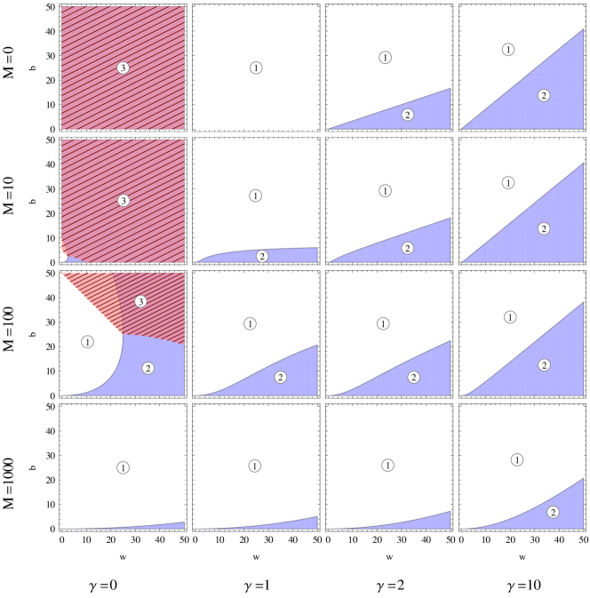
Refer to caption
Figure 2: The behavior of $Q_{\text{$M$,$\gamma$}}$ for varying parameter values. The graph consists of two subgraphs with $w$ internal weight each, connected by an edge with weigh $b$. Hence the volume of the total graph is $2w+2b$. In region (1) the optimal clustering has a single cluster, In region (2) (light blue) the optimal clustering separates the subgraphs. In region (3) (red, hatched) the subgraphs themselves will be split apart.

In Figure 2 we show which graphs give which outcomes for adaptive scale modularity with various parameter settings. The first column, $\gamma=0$, is of particular interest, since it corresponds to fixed scale modularity and hence also to $Q_{\text{RB}}$ and to modularity in certain graphs. In the third row we can see that when $2v=2w+2b>M=100$ the cliques are split apart. This is precisely the region in which monotonicity no longer holds. Overall, the parameter $M$ has the effect of determining the scale; each row in this figure is merely the previous row magnified by a factor $10$. Increasing $M$ has the effect of merging small clusters. On the other hand, the $\gamma$ parameter controls the slope of the boundary between outcomes (1) and (2), i.e. the fraction of edges that should be within a cluster. This is most clearly seen when $M=0$, while otherwise the effect of $M$ dominates for small clusters.

7 Conclusion and Open Questions

Permutation invariance

Scale invariance

Scale invariance (family)

Richness

Monotonicity

Locality

Continuity

Connected components $\checkmark$ $\checkmark$ n.a. $\checkmark$ $\checkmark$ $\checkmark$ $-$
Modularity $\checkmark$ $\checkmark$ n.a. $\checkmark$ $-$ $-$ $\checkmark$
Reichardt and Bornholdt (2004) $\checkmark$ $\checkmark$ $\checkmark$ $\checkmark$ $-$ $-$ $\checkmark$
Fixed scale modularity $\checkmark$ $M=0$ $\checkmark$ $\checkmark$ $-$ $\checkmark$ $\checkmark$
Adaptive scale modularity $\checkmark$ $M=0$ $\checkmark$ $\gamma\geq 1$ $\gamma\geq 2$ $\checkmark$ $\checkmark$
Constant Potts Model (Traag et al., 2011) $\checkmark$ $-$ $\checkmark$ $\gamma>0$ $\checkmark$ $\checkmark$ $\checkmark$
Normalized cut $\checkmark$ $\checkmark$ n.a. $-$ $\checkmark$ $\checkmark$ $\checkmark$
Table 1: Overview of quality functions discussed in this paper and the properties they satisfy.

In this paper we presented an axiomatic framework for graph clustering quality functions consisting of six properties. We showed that modularity does not satisfy the monotonicity property. This motivated the derivation of a new family of quality functions, adaptive scale modularity, that satisfies all properties and has standard graph clustering quality functions as special cases. Results of an experimental parameter dependence analysis showed the high flexibility of adaptive scale modularity. However, adaptive scale modularity should not be considered the solution to all the problems of modularity, but rather an example of how axioms can be used in practice.

An overview of the discussed axioms and quality functions can be found in table 1. Many more quality functions have been proposed in the literature, so this list is by no means exhaustive. An interesting topic for future research is to make a survey of which existing quality functions satisfy which of the proposed properties.

We also investigated resolution-limit-free quality functions as defined in (Traag et al., 2011). As illustrated in section 6.2, adaptive scale modularity allows to perform clustering at various resolutions, by varying the values of its two parameters. However it is not resolution-limit-free.

Our paper did not address questions such as finding a best quality function (Almeida, Guedes, Jr., and Zaki, 2011), or selecting a significant resolution scale (Traag et al., 2013). The aim was to provide necessary conditions about what a good quality function is, in order to rule out and/or to improve quality functions. The proposed axioms and the introduction of adaptive scale modularity are an effort in this direction.

We also did not address the question of finding a clustering with the highest quality. Finding the optimal value of quality functions such as modularity is NP-hard (Brandes et al., 2008), but several heuristic and approximation algorithms have been developed. One class of algorithms uses a divisive approach, see for instance Newman (2006); Ruan and Zhang (2008). For such a tactic to be valid, an optimal or close to optimal clustering of a subgraph should also be a near optimal clustering of the entire graph. This is ensured by locality. Recently Dinh and Thai (2013) proposed polynomial-time approximation algorithms for the modularity maximization in the context of scale free networks. It would be interesting to investigate the suitability of these algorithms for adaptive scale modularity maximization.

In this work we have only looked at non-negative weights, undirected graphs, and only at hard partitioning. An extension to graphs with negative weights, to directed graphs and to overlapping clusters remains to be investigated. Another open problem is how to use these axioms for reasoning about quality functions and clustering algorithms.

Acknowledgments

We thank the reviewers for their comments. This work has been partially funded by the Netherlands Organization for Scientific Research (NWO) within the NWO project 612.066.927.

A Proof of Theorem 3 (Modularity is Rich)

The proofs of richness rely on clique graphs,

Definition 7 (Clique graph)

Let $V$ be a set of nodes, $C$ be a partition of $V$, and $k$ be a positive constant. The clique graph of $C$ with edge weight $k$ is defined as $G=(V,E)$ where $E(i,j)=k$ if $i\sim_{C}j$ and $E(i,j)=0$ otherwise.

Proof

Let $V$ be a set of nodes and $C\neq\{V\}$ be a clustering of $V$. Let $G=(V,E)$ be a clique graph of $C$ with edge weight $1$. Note that $E(i,i)=1$, so any possible cluster will have a positive volume. Let $D$ be a clustering of $G$ with maximal modularity.

Suppose that there is a cluster $d\in D$ that contains $i,j\in d$ with $i\not\sim_{C}j$. Then we can split the cluster into $d_{1}=\{k\in d\mid k\sim_{C}i\}$ and $d_{2}=\{k\in d\mid k\not\sim_{C}i\}$. Because there are no edges between nodes in $d_{1}$ and nodes in $d_{2}$, it is the case that $w_{d}=w_{d_{1}}+w_{d_{2}}$. Both $d_{1}$ and $d_{2}$ are non-empty and have a positive volume, so $v_{d}^{2}=(v_{d_{1}}+v_{d_{2}})^{2}<v_{d_{1}}^{2}+v_{d_{2}}^{2}$. Therefore $Q_{\text{modularity}}(G,D)<Q_{\text{modularity}}(G,D\setminus\{d\}\cup\{d_{1},d_{2}\})$. So $D$ does not have maximal modularity, which is a contradiction.

Suppose, on the other hand that all clusters $d\in D$ are a subset of some cluster in $C$, i.e. $D$ is a refinement of $C$. Then either $D=C$, or there are two clusters $d_{1},d_{2}\in D$ that are both a subset of the same cluster $c\in C$. In the latter case we can combine the two clusters into $d=d_{1}\cup d_{2}$. The within weight of this combined cluster is $w_{d}=|d|^{2}=w_{d_{1}}+w_{d_{2}}+2|d_{1}||d_{2}|$. The squared volume of the combined cluster is $v_{d}^{2}=|d|^{2}|c|^{2}=v_{d_{1}}^{2}+v_{d_{2}}^{2}+2|d_{1}||d_{2}||c|^{2}$. So this changes increases the modularity by

$\displaystyle Q_{\text{modularity}}(G,D\setminus\{d_{1},d_{2}\}\cup\{d\})-Q_{\text{modularity}}(G,D)$
$\displaystyle\quad=2|d_{1}||d_{2}|/v_{V}-2|d_{1}||d_{2}||c|^{2}/v_{V}^{2}$
$\displaystyle\quad=2|d_{1}||d_{2}|(v_{V}-|c|^{2})/v_{V}^{2}>0,$

which contradicts the assumption that $D$ has maximal modularity. Therefore the only optimal clustering of $G$ is $C$. Note that the above inequality only holds when $|c|^{2}=v_{c}<v_{V}$, which is the case because $C\neq\{V\}$.

When $C=\{V\}$, a clique graph will not work; because both $\{V\}$ and the clustering that assigns half the nodes to one cluster, and half to another have modularity equal to 00. In this case, instead define $G=(V,E)$ by $E(i,j)=1$ if $i\neq j$ and 00 if $i=j$. Then the modularity for $C$ is $q(G,\{V\})=0$. Any cluster $d$ in a clustering $D$ will have $v_{d}=|d|(|V|-1)$ and $w_{d}=|d|(|d|-1)$. Therefore the contribution of this cluster to the total quality is $-|d|(|V|-|d|)/(|V|^{2}(|V|-1))$, which is negative when $|d|<|V|$. So the modularity of any clustering other than $\{V\}$ will be negative, hence $\{V\}$ is the only optimal clustering.

Since for every $C$ we can construct a graph where $C$ is the only optimal clustering, modularity is rich.


B Proof of Theorem 8 (Adaptive Scale Modularity is Rich)

Denote by $f_{C}(d)$ the largest fraction of any cluster from $C$ that is contained in a cluster $d$.

$\displaystyle f_{C}(d)=\max_{c\in C}\frac{|c\cap d|}{|c|}.$

For any clustering $D$ we have that

$\displaystyle\sum_{d\in D}f_{C}(d)=\sum_{d\in D}\max_{c\in C}\frac{|c\cap d|}{|c|}\leq\sum_{d\in D}\sum_{c\in C}\frac{|c\cap d|}{|c|}=|C|.$ (5)

And since $f_{C}(d)\leq 1$ for all clusters $d$, we also have that

$\displaystyle\sum_{d\in D}f_{C}(d)\leq|D|.$ (6)
Lemma 11

For a clique graph of $C$ it is the case that $w_{d}/v_{d}\leq f_{C}(d)$.

Proof  Given a cluster $d$ and a clique graph $G$ of $C$ with weight $k>0$, the volume of $d$ is

$$v_{d}=\sum_{c\in C}k|c\cap d||c|,$$

and the within cluster weight is

$$w_{d}=\sum_{c\in C}k|c\cap d|^{2}.$$

Therefore

$\displaystyle w_{d}\leq\sum_{c\in C}k|c\cap d||c|f_{C}(d)=v_{d}f_{C}(d).$

And hence $w_{d}/v_{d}\leq f_{C}(d)$.  

Lemma 12

Let $G$ be the clique graph of a clustering $C$ with weight $k$, and let $0<\beta<1$ be a constant. Then $\sum_{d\in D}(w_{d}/v_{d}-\beta)=(1-\beta)|C|$ if $D=C$, while $\sum_{d\in D}(w_{d}/v_{d}-\beta)<(1-\beta)|C|-\epsilon$ if $D\neq C$, where $\epsilon=\min(\beta,1-\beta,1/|V|)/2$.

Proof  Suppose that $D=C$, then for every cluster $c\in C$, $w_{c}=v_{c}=k|c|^{2}$, and so

$$\sum_{c\in C}\Bigl{(}\frac{w_{d}}{v_{d}}-\beta\Bigr{)}=(1-\beta)|C|.$$

Otherwise, $D\neq C$. Assume that $\sum_{d\in D}(w_{d}/v_{d}-\beta)\geq(1-\beta)|C|-\min(\beta,1/|V|)/2$. By Lemma 11,

$\displaystyle|C|-\beta(|C|+1)$
$\displaystyle<$ $\displaystyle|C|-\beta|C|-\epsilon$
$\displaystyle\leq$ $\displaystyle\sum_{d\in D}(\frac{w_{d}}{v_{d}}-\beta)$
$\displaystyle\leq$ $\displaystyle\sum_{d\in D}(f_{C}(d)-\beta)$
$\displaystyle\leq$ $\displaystyle|C|-\beta|D|.$

Since $\beta>0$, this implies that $|D|<|C|+1$.

Additionally, since $f_{C}(d)\leq 1$ for all clusters $d\in D$,

$\displaystyle(1-\beta)(|C|-1)$
$\displaystyle<$ $\displaystyle(1-\beta)|C|-\epsilon$
$\displaystyle\leq$ $\displaystyle\sum_{d\in D}(f_{C}(d)-\beta)$
$\displaystyle\leq$ $\displaystyle(1-\beta)|D|$

Since $\beta<1$, this implies that $|D|>|C|-1$. Hence $|D|=|C|$.

Suppose that $f_{C}(d)<1$ for some $d\in D$, which implies that $|c\cap d|<|c|$. Because edges are discrete, this can only happen when $|c\cap d|\leq|c|-1$ for all clusters $c$. And the size of clusters is bounded by $|c|\leq|V|$. Hence $f_{C}(d)\leq(|V|-1)/|V|=1-1/|V|$. And since for all other clusters $d^{\prime}$, $f_{C}(d^{\prime})\leq 1$, we then have

$\displaystyle\sum_{d\in D}(f_{C}(d)-\beta)$
$\displaystyle\leq$ $\displaystyle(1-\beta)|D|-1/|V|$
$\displaystyle<$ $\displaystyle(1-\beta)|C|-\epsilon$
$\displaystyle\leq$ $\displaystyle\sum_{d\in D}(w_{d}/v_{d}-\beta)$
$\displaystyle\leq$ $\displaystyle\sum_{d\in D}(f_{C}(d)-\beta),$

which is a contradiction. Hence, it must be the case that $f_{C}(d)=1$ for all clusters $d\in D$. By the definition of $f_{C}$ this means that for every $d$ there is a cluster $c\in C$ such that $|c\cap d|=|c|$, and therefore $c\subseteq d$. Since the clusters are disjoint and $|D|=|C|$, this implies that $D=C$. Which is a contradiction, so $\sum_{d\in D}(w_{d}/v_{d}-\beta)<(1-\beta)|C|-\epsilon$.  

When $M=0$, the adaptive scale modularity reduces to $w_{d}/(\gamma v_{d})-|D|/\gamma^{2}$, and the above lemma is enough to prove richness. For non-zero values of $M$, we can get ‘close enough’ by choosing large enough edge weights. This is formalized in the following lemma.

Lemma 13

Let $d$ be a cluster in a clustering of a clique graph of $C$ with weight $k$. Then

$\displaystyle\frac{w_{d}}{v_{d}}-\beta-\beta M/k\leq q(d)/\beta\leq\frac{w_{d}}{v_{d}}-\beta+2\beta^{2}M/k,$

where

$$q(d)=\frac{w_{d}}{M+v_{d}/\beta}-\Bigl{(}\frac{v_{d}}{M+v_{d}/\beta}\Bigr{)}^{2}$$

denotes the contribution of $d$ to the $M$-adaptive modularity.

Proof  Since clusters are non-empty, and in a clique graph $E(i,i)=k$, it follows that $v_{d}\geq w_{d}\geq k$. So

$\displaystyle q(d)/\beta$
$\displaystyle=$ $\displaystyle\frac{\beta Mw_{d}+v_{d}w_{d}-\beta v_{d}^{2}}{(\beta M+v_{d})^{2}}$
$\displaystyle=$ $\displaystyle\frac{w_{d}}{v_{d}}-\beta+\frac{\beta^{2}M(\beta M+2v_{d})-\beta^{2}M^{2}w_{d}/v_{d}-\beta Mw_{d}}{(\beta M+v_{d})^{2}}$
$\displaystyle\leq$ $\displaystyle\frac{w_{d}}{v_{d}}-\beta+\frac{\beta^{2}M(\beta M+2v_{d})}{(\beta M+v_{d})^{2}}$
$\displaystyle\leq$ $\displaystyle\frac{w_{d}}{v_{d}}-\beta+\frac{2\beta^{2}M(\beta M+2v_{d})}{(\beta M+v_{d})(\beta M+2v_{d})}$
$\displaystyle=$ $\displaystyle\frac{w_{d}}{v_{d}}-\beta+\frac{2\beta^{2}M}{\beta M+v_{d}}$
$\displaystyle\leq$ $\displaystyle\frac{w_{d}}{v_{d}}-\beta+\frac{2\beta^{2}M}{k}.$

And since $w_{d}\leq v_{d}$,

$\displaystyle q(d)/\beta$
$\displaystyle=$ $\displaystyle\frac{w_{d}}{v_{d}}-\beta+\frac{\beta^{2}M(\beta M+2v_{d})-\beta^{2}M^{2}w_{d}/v_{d}-\beta Mw_{d}}{(\beta M+v_{d})^{2}}$
$\displaystyle\geq$ $\displaystyle\frac{w_{d}}{v_{d}}-\beta-\frac{\beta^{2}M^{2}+\beta Mv_{d}}{(\beta M+v_{d})^{2}}$
$\displaystyle=$ $\displaystyle\frac{w_{d}}{v_{d}}-\beta-\frac{\beta M}{\beta M+v_{d}}$
$\displaystyle\geq$ $\displaystyle\frac{w_{d}}{v_{d}}-\beta-\frac{\beta M}{k}.$


Combining these lemmas yields the proof of the general theorem:

Proof  Given a clustering $C$. Define $\beta=1/\gamma$. If $\gamma>1$ then $0<\beta<1$. Pick $k>3|V|\beta^{2}M/\epsilon$ where $\epsilon$ is defined as in Lemma 12.

Let $G$ be the clique graph of $C$ with weight $k$. Let $D\neq C$ be a clustering of $G$. Then by Lemmas 12 and 13,

$\displaystyle Q_{\text{$M$,$\gamma$}}(G,D)/\beta$
$\displaystyle=$ $\displaystyle\sum_{d\in D}q(d)$
$\displaystyle\leq$ $\displaystyle\sum_{d\in D}(w_{d}/v_{d}-\beta+2\beta^{3}M/k)$
$\displaystyle\leq$ $\displaystyle(1-\beta)|C|+2|D|\beta^{3}M/k-\epsilon$
$\displaystyle\leq$ $\displaystyle(1-\beta)|C|+2|V|\beta^{2}M/k-\epsilon$
$\displaystyle<$ $\displaystyle(1-\beta)|C|-|V|\beta^{2}M/k$
$\displaystyle\leq$ $\displaystyle(1-\beta)|C|-|C|\beta^{2}M/k$
$\displaystyle=$ $\displaystyle\sum_{c\in C}(w_{c}/v_{c}-\beta+\beta^{2}M/k)$
$\displaystyle\leq$ $\displaystyle Q_{\text{$M$,$\gamma$}}(C)/\beta.$

Hence the quality is maximal for $C$. Since there is a clique graph and $k$ for every clustering, adaptive scale modularity is rich.  

C Proof of Theorem 9 (Adaptive Scale Modularity is Monotonic)

Proof 

Given a constants $M>0$ and $\gamma\geq 2$, a graph $G$ and a clustering $C$ of $G$. Let $c\in C$ be any cluster. Writing the volume of $c$ as $v_{c}=w_{c}+b_{c}$, the contribution of this cluster to the quality of $G$ is $q(w_{c},b_{c})$ where

$\displaystyle q(w,b)$ $\displaystyle=\frac{w}{M+\gamma w+\gamma b}-\Bigl{(}\frac{w+b}{M+\gamma w+\gamma b}\Bigr{)}^{2}.$

The partial derivatives of $q$ are

$\displaystyle\frac{\partial q(w,b)}{\partial w}$ $\displaystyle=\frac{M^{2}+(\gamma-2)M(w+b)+\gamma b(M+\gamma w+\gamma b)}{(M+\gamma w+\gamma b)^{3}}\geq 0$
$\displaystyle\frac{\partial q(w,b)}{\partial b}$ $\displaystyle=-\frac{\gamma wM+(w+b)(M+\gamma^{2}w)}{(M+\gamma w+\gamma b)^{3}}\leq 0.$

This means that $q$ is a monotonically non-decreasing function in $w$ and a non-increasing function in $b$.

For any graph $G^{\prime}$ that is a $C$-consistent change of $G$, it holds that $w^{\prime}_{c}\geq w_{c}$ and $b^{\prime}_{c}\leq b_{c}$. So $q(w^{\prime}_{c},b^{\prime}_{c})\geq q(w_{c},b_{c})$. And therefore $Q_{\text{$M$,$\gamma$}}(G^{\prime},C)\geq Q_{\text{$M$,$\gamma$}}(G,C)$. So adaptive scale modularity is monotonic.  

References

  • Ackerman et al. (2013) M. Ackerman, S. Ben-David, D. Loker, and S. Sabato. Clustering oligarchies. In Proceedings of the International Conference on Artificial Intelligence and Statistics (AISTATS), volume 31 of JMLR Workshop and Conference Proceedings, pages 66–74, 2013.
  • Ackerman and Ben-David (2008) Margareta Ackerman and Shai Ben-David. Measures of clustering quality: A working set of axioms for clustering. In Daphne Koller, Dale Schuurmans, Yoshua Bengio, and Léon Bottou, editors, NIPS, pages 121–128. Curran Associates, Inc., 2008.
  • Ackerman and Ben-David (2013) Margareta Ackerman and Shai Ben-David. A characterization of linkage-based hierarchical clustering. Journal of Machine Learning Research, 2013.
  • Ackerman et al. (2010a) Margareta Ackerman, Shai Ben-David, and David Loker. Towards property-based classification of clustering paradigms. In John D. Lafferty, Christopher K. I. Williams, John Shawe-Taylor, Richard S. Zemel, and Aron Culotta, editors, NIPS, pages 10–18. Curran Associates, Inc., 2010a.
  • Ackerman et al. (2010b) Margareta Ackerman, Shai Ben-David, and David Loker. Characterization of linkage-based clustering, 2010b.
  • Ackerman et al. (2012) Margareta Ackerman, Shai Ben-David, Simina Brânzei, and David Loker. Weighted clustering. In Jörg Hoffmann and Bart Selman, editors, AAAI. AAAI Press, 2012.
  • Almeida et al. (2011) Helio Almeida, Dorgival Guedes, Wagner Meira Jr., and Mohammed J. Zaki. Is there a best quality metric for graph clusters? In Dimitrios Gunopulos, Thomas Hofmann, Donato Malerba, and Michalis Vazirgiannis, editors, Machine Learning and Knowledge Discovery in Databases, volume 6911 of Lecture Notes in Computer Science, pages 44–59. Springer Berlin Heidelberg, 2011. ISBN 978-3-642-23779-9.
  • Blondel et al. (2008) Vincent D. Blondel, Jean-Loup Guillaume, Renaud Lambiotte, and Etienne Lefebvre. Fast unfolding of communities in large networks. J. Stat. Mech. Theory Exp., 2008(10):P10008, 2008. ISSN 1742-5468. doi: 10.1088/1742-5468/2008/10/P10008. URL http://dx.doi.org/10.1088/1742-5468/2008/10/P10008.
  • Bollobás (2001) Béla Bollobás. The Evolution of Random Graphs – the Giant Component, pages 130–159. Cambridge University Press, 2001. ISBN 9780521797221.
  • Brandes et al. (2008) Ulrik Brandes, Daniel Delling, Marco Gaertler, Robert Gorke, Martin Hoefer, Zoran Nikoloski, and Dorothea Wagner. On modularity clustering. IEEE Transactions on Knowledge and Data Engineering, 20(2):172–188, 2008. ISSN 1041-4347. doi: 10.1109/TKDE.2007.190689.
  • Bubeck and Luxburg (2009) Sébastien Bubeck and Ulrike von Luxburg. Nearest neighbor clustering: A baseline method for consistent clustering with arbitrary objective functions. J. Mach. Learn. Res., 10:657–698, June 2009. ISSN 1532-4435. URL http://dl.acm.org/citation.cfm?id=1577069.1577092.
  • Carlsson et al. (2013) Gunnar Carlsson, Facundo Mémoli, Alejandro Ribeiro, and Santiago Segarra. Axiomatic construction of hierarchical clustering in asymmetric networks. CoRR, abs/1301.7724, 2013.
  • Dinh and Thai (2013) Thang N. Dinh and My T. Thai. Community detection in scale-free networks: Approximation algorithms for maximizing modularity. IEEE Journal on Selected Areas in Communications, 31(6):997–1006, 2013.
  • Fortunato and Barthélemy (2007) Santo Fortunato and Marc Barthélemy. Resolution limit in community detection. Proc. Natl. Acad. Sci. USA, 104(1):36–41, 2007. doi: 10.1073/pnas.0605965104.
  • Gollapudi and Sharma (2009) Sreenivas Gollapudi and Aneesh Sharma. An axiomatic approach for result diversification. In Proceedings of the 18th international conference on World wide web, pages 381–390, 2009.
  • Good et al. (2010) Benjamin H. Good, Yves A. de Montjoye, and Aaron Clauset. Performance of modularity maximization in practical contexts. Phys. Rev. E, 81(4):046106, April 2010. doi: 10.1103/PhysRevE.81.046106. URL http://dx.doi.org/10.1103/PhysRevE.81.046106.
  • Kleinberg (2002) Jon M. Kleinberg. An impossibility theorem for clustering. In Suzanna Becker, Sebastian Thrun, and Klaus Obermayer, editors, NIPS, pages 446–453. MIT Press, 2002. ISBN 0-262-02550-7.
  • Lancichinetti and Fortunato (2011) Andrea Lancichinetti and Santo Fortunato. Limits of modularity maximization in community detection. Phys. Rev. E, 84:066122, December 2011. doi: 10.1103/PhysRevE.84.066122. URL http://dx.doi.org/10.1103/PhysRevE.84.066122.
  • Meila (2005) Marina Meila. Comparing clusterings: an axiomatic view. In Proceedings of the 22nd international conference on Machine learning, pages 577–584. ACM, 2005.
  • Newman (2006) Mark E. J. Newman. Finding community structure in networks using the eigenvectors of matrices. Phys. Rev. E, 74(3):036104, July 2006. doi: 10.1103/PhysRevE.74.036104. URL http://dx.doi.org/10.1103/PhysRevE.74.036104.
  • Newman and Girvan (2004) Mark E. J. Newman and Michelle Girvan. Finding and evaluating community structure in networks. Phys. Rev. E, 69:026113, Feb 2004. doi: 10.1103/PhysRevE.69.026113. URL http://pre.aps.org/abstract/PRE/v69/i2/e026113.
  • Puzicha et al. (1999) Jan Puzicha, Thomas Hofmann, and Joachim M. Buhmann. A theory of proximity based clustering: Structure detection by optimization. Pattern Recognition, 33:617–634, 1999.
  • Reichardt and Bornholdt (2004) Jörg Reichardt and Stefan Bornholdt. Detecting fuzzy community structures in complex networks with a Potts model. Phys. Rev. Lett., 93:218701, 2004. doi: 10.1103/PhysRevLett.93.218701.
  • Reichardt and Bornholdt (2006) Jörg Reichardt and Stefan Bornholdt. Statistical mechanics of community detection. Physical Review E, 74(1):016110, 2006.
  • Reichardt and Bornholdt (2007) Jörg Reichardt and Stefan Bornholdt. Partitioning and modularity of graphs with arbitrary degree distribution. Phys. Rev. E, 76:015102, Jul 2007. doi: 10.1103/PhysRevE.76.015102. URL http://link.aps.org/doi/10.1103/PhysRevE.76.015102.
  • Ruan and Zhang (2008) Jianhua Ruan and Weixiong Zhang. Identifying network communities with a high resolution. Phys. Rev. E, 77:016104, Jan 2008. doi: 10.1103/PhysRevE.77.016104. URL http://link.aps.org/doi/10.1103/PhysRevE.77.016104.
  • Shi and Malik (2000) Jianbo Shi and Jitendra Malik. Normalized cuts and image segmentation. volume 22, pages 888–905, Washington, DC, USA, August 2000. IEEE Computer Society. doi: 10.1109/34.868688. URL http://dx.doi.org/10.1109/34.868688.
  • Traag et al. (2011) Vincent A. Traag, Paul Van Dooren, and Yurii E. Nesterov. Narrow scope for resolution-limit-free community detection. Phys. Rev. E, 84:016114, Jul 2011. doi: 10.1103/PhysRevE.84.016114. URL http://link.aps.org/doi/10.1103/PhysRevE.84.016114.
  • Traag et al. (2013) Vincent A. Traag, Gautier Krings, and Paul Van Dooren. Significant scales in community structure. Submitted, Jun 2013. URL http://arxiv.org/abs/1306.3398.
  • van Laarhoven and Marchiori (2013) Twan van Laarhoven and Elena Marchiori. Graph clustering with local search optimization: The resolution bias of the objective function matters most. Phys. Rev. E, 87:012812, Jan 2013. doi: 10.1103/PhysRevE.87.012812. URL http://link.aps.org/doi/10.1103/PhysRevE.87.012812.
  • Zadeh and Ben-David (2009) Reza Bosagh Zadeh and Shai Ben-David. A uniqueness theorem for clustering. In Proceedings of the Twenty-Fifth Conference on Uncertainty in Artificial Intelligence, UAI ’09, pages 639–646, Arlington, Virginia, United States, 2009. AUAI Press. ISBN 978-0-9749039-5-8. URL http://dl.acm.org/citation.cfm?id=1795114.1795189.