A pricing measure to explain the risk premium in power markets

Abstract.

In electricity markets, it is sensible to use a two-factor model with mean reversion for spot prices. One of the factors is an Ornstein-Uhlenbeck (OU) process driven by a Brownian motion and accounts for the small variations. The other factor is an OU process driven by a pure jump Lévy process and models the characteristic spikes observed in such markets. When it comes to pricing, a popular choice of pricing measure is given by the Esscher transform that preserves the probabilistic structure of the driving Lévy processes, while changing the levels of mean reversion. Using this choice one can generate stochastic risk premiums (in geometric spot models) but with (deterministically) changing sign. In this paper we introduce a pricing change of measure, which is an extension of the Esscher transform. With this new change of measure we also can slow down the speed of mean reversion and generate stochastic risk premiums with stochastic non constant sign, even in arithmetic spot models. In particular, we can generate risk profiles with positive values in the short end of the forward curve and negative values in the long end. Finally, our pricing measure allows us to have a stationary spot dynamics while still having randomly fluctuating forward prices for contracts far from maturity.

1. Introduction

In modelling and analysis of forward and futures prices in commodity markets, the risk premium plays an important role. It is defined as the difference between the forward price and the expected commodity spot price at delivery, and the classical theory predicts a negative risk premium. The economical argument for this is that producers of the commodity is willing to pay a premium for hedging their production (see Geman [9] for a discussion, as well as a list of references).

Geman and Vasicek  [10] argued that in power markets, the consumers may hedge the price risk using forward contracts which are close to delivery, and thus creating a positive premium. Power is a non-storable commodity, and as such may experience rather large price variations over short time (sometimes referred to as spikes). One might observe a risk premium which may be positive in the short end of the forward market, and negative in the long end where the producers are hedging their power generation. A theoretical and empirical foundation for this is provided in, for example, Bessembinder and Lemon [5] and Benth, Cartea and Kiesel [3].

When deriving the forward price, one specifies a pricing probability and computes the forward price as the conditional expected spot at delivery. In the power market, this pricing probability is not necessarily a so-called equivalent martingale measure, or a risk neutral probability (see Bingham and Kiesel [6]), as the spot is not tradeable in the usual sense. Thus, a pricing probability can a priori be any equivalent measure, and in effect is an indirect specification of the risk premium. In this paper we suggest a new class of pricing measures which gives a stochastically varying risk premium.

We will focus our considerations on the power market, where typically a spot price model may take the form as a two-factor mean reversion dynamics. Lucia and Schwartz [20] considered two-factor models for the electricity spot price dynamics in the Nordic power market NordPool. Both arithmetic and geometric models where suggested, that is, either directly modelling the spot price by a two-factor dynamics, or assuming such a model for the logarithmic spot prices. Their models were based on Brownian motion and, as such, not able to capture the extreme variations in the power spot markets. Cartea and Figueroa [7] used a compound Poisson process to model spikes, that is, extreme price jumps which are quickly reverted back to ”normal levels”. Benth, Šaltytė Benth and Koekebakker [2] give a general account on multi-factor models based on Ornstein-Uhlenbeck processes driven by both Brownian motion and Lévy processes. Empirical studies suggest a stationary power spot price dynamics after explaining deterministic seasonal variations (see e.g. Barndorff-Nielsen, Benth and Veraart [1] for a study of spot prices at EEX, the German power exchange). We will in this paper focus on a two-factor model for the spot, where each factor is an Ornstein-Uhlenbeck process, driven by a Brownian motion and a jump process, respectively. The first factor models the ”normal variations” of the spot price, whereas the second accounts for sudden jumps (spikes) due to unexpected imbalances in supply and demand.

The standard approach in power markets is to specify a pricing measure which is preserving the Lévy property. This is called the Esscher transform (see Benth et al. [2]), and works for Lévy processes as the Girsanov transform with a constant parameter for Brownian motion. The effect of doing such a measure change is to adjust the mean reversion level, and it is known that the risk premium becomes deterministic and typically either positive or negative for all maturities along the forward curve.

We propose a class of measure changes which slows down the speed of mean reversion of the two factors. As it turns out, in conjunction with an Esscher transform as mentioned above, we can produce a stochastically varying risk premium, where potential positive premiums in the short end of the market can be traced back to sudden jumps in the spike factor being slowed down under the pricing measure. This result holds for arithmetic spot models, whereas the geometric ones are much harder to analyse under this change of probability. The class of probabilities preserves the Ornstein-Uhlenbeck structure of the factors, and as such may be interpreted as a dynamic structure preserving measure change. For the Lévy driven component, the Lévy property is lost in general, and we obtain a rather complex jump process with state-dependent (random) compensator measure.

We can explicitly describe the density process for our measure change. The theoretical contribution of this paper, besides the new insight on risk premium, is a proof that the density process is a true martingale process, indeed verifying that we have constructed a probability measure. This verification is not straightforward because the kernels used to define the density process, through stochastic exponentiation, are stochastic and unbounded. Hence, the usual criterion by Lépingle-Mémin [19] is difficult to apply and, furthermore, it does not provide sharp results. We follow the same line of reasoning as in a very recent paper by Klebaner and Lipster [18]. Although their result is more general than ours in some respects, it does not apply directly to our case because we need some additional integrability requirements. The proof is roughly as follows. First, we reduce the problem to show the uniform integrability of the sequence of random variables obtained by evaluating at the end of the trading period the localised density process. This sequence of random variables naturally induces a sequence of measure changes which, combined with an easy inequality for the logarithm function, allow us to get rid of the stochastic exponential in the expression to be bounded. Finally, we can reduce the problem to get an uniform bound for the second moment of the factors under these new probability measures.

Interestingly, as our pricing probability is reducing the speed of mean reversion, we might in the extreme situation ”turn off” the mean reversion completely (by reducing it to zero). For example, if we take the Brownian factor as the case, we can have a stationary dynamics of the ”normal variations” in the market, but when looking at the process under the pricing probability the factor can be non-stationary, that is, a drifted Brownian motion. A purely stationary dynamics for the spot will produce constant forward prices in the long end of the market, something which is not observed empirically. Hence, the inclusion of non-stationary factors are popular in modelling the spot-forward markets. In many studies of commodity spot and forward markets, one is considering a two-factor model with one non-stationary and one stationary component. The stationary part explains the short term variations, while the non-stationary is supposed to account for long-term price fluctuations in the spot (see Gibson and Schwartz [11] and Schwartz and Smith [23] for such models applied to oil markets). Indeed, the power spot models in Lucia and Schwartz [20] are of this type. It is hard to detect the long term factor in spot price data, and one is usually filtering it out from the forward prices using contracts far from delivery. Theoretically, such contracts should have a dynamics being proportional to the long term factor. Contrary to this approach, one may in view of our new results, suggest a stationary spot dynamics and introduce a pricing measure which turns one of the factors into a non-stationary dynamics. This would imply that one could directly fit a two-factor stationary spot model to power data, and next calibrate a measure change to account for the long term variations in the forward prices by turning off (or significantly slow down) the speed of mean reversion.

Our results are presented as follows: in the next section we introduce the basic assumptions and properties satisfied by the factors in our model. Then, in Section 3, we define the new change of measure and prove the main results regarding the uniform integrability of its density process. We deal with the Brownian and pure jump case separately. Finally, in Section 4, we recall the arithmetic and geometric spot price models. We compute the forward price processes induced by this change of measure and we discuss the risk premium profiles that can be obtained.

2. The mathematical set up

Suppose that $(\Omega,\mathcal{F},\{\mathcal{F}_{t}\}_{t\in[0,T]},P)$ is a complete filtered probability space, where $T>0$ is a fixed finite time horizon. On this probability space there are defined $W$, a standard Wiener process, and $L,$ a pure jump Lévy subordinator with finite expectation, that is a Lévy process with the following Lévy-Itô representation $L(t)=\int_{0}^{t}\int_{0}^{\infty}zN^{L}(ds,dz),t\in[0,T],$ where $N^{L}(ds,dz)$ is a Poisson random measure with Lévy measure $\ell$ satisfying $\int_{0}^{\infty}z\ell(dz)<\infty.$ We shall suppose that $W$ and $L$ are independent of each other. The following assumption is minimal, having in mind, on the one hand, that our change of measure extends the Esscher transform and, on the other hand, that we are going to consider a geometric spot price model.

Assumption 1.

We assume that

$$\Theta_{L}\triangleq\sup\{\theta\in\mathbb{R}_{+}:\mathbb{E}[e^{\theta L(1)}]<\infty\},$$ (2.1)

is strictly positive constant, which may be $\infty.$

Actually, to have the geometric model well defined we will need to assume later that $\Theta_{L}>1.$ Some remarks are in order.

Remark 2.1.

In $(-\infty,\Theta_{L})$ the cumulant (or log moment generating) function $\kappa_{L}(\theta)\triangleq\log\mathbb{E}_{P}[e^{\theta L(1)}]$ is well defined and analytic. As $0\in(-\infty,\Theta_{L})$, $L$ has moments of all orders. Also, $\kappa_{L}(\theta)$ is convex, which yields that $\kappa_{L}^{\prime\prime}(\theta)\geq 0$ and, hence, that $\kappa_{L}^{\prime}(\theta)$ is non decreasing. Finally, as a consequence of $L\geq 0,$ a.s., we have that $\kappa_{L}^{\prime}(\theta)$ is non negative.

Remark 2.2.

Thanks to the Lévy-Kintchine representation of $L$ we can express $\kappa_{L}(\theta)$ and its derivatives in terms of the Lévy measure $\ell.$ We have that for $\theta\in(-\infty,\Theta_{L})$

$$\kappa_{L}(\theta) =\int_{0}^{\infty}(e^{\theta z}-1)\ell(dz)<\infty,$$

$$\kappa_{L}^{(n)}(\theta) =\int_{0}^{\infty}z^{n}e^{\theta z}\ell(dz)<\infty,\quad n\in\mathbb{N},$$

showing, in fact, that $\kappa_{L}^{(n)}(\theta)>0,n\in\mathbb{N}.$

Consider the OU processes

$$X(t) =X(0)+\int_{0}^{t}(\mu_{X}-\alpha_{X}X(s))ds+\sigma_{X}W(t)\quad t\in[0,T],$$ (2.2)

$$Y(t) =Y(0)+\int_{0}^{t}(\mu_{Y}-\alpha_{Y}Y(s))ds+L(t),\quad t\in[0,T],$$ (2.3)

with $\alpha_{X},\sigma_{X},\alpha_{Y}>0,\mu_{X},X(0)\in\mathbb{R},\mu_{Y},Y(0)\geq 0.$ Note that, in equation $\left(\ref{Equ_OU_Brownian}\right),$ $X$ is written as a sum of a finite variation process and a martingale. We may also rewrite equation $(\ref{Equ_OU_Levy})$ as a sum of a finite variation part and pure jump martingale

$$Y(t)=Y(0)+\int_{0}^{t}(\mu_{Y}+\kappa_{L}^{\prime}(0)-\alpha_{Y}Y(s))ds+\int_{0}^{t}\int_{0}^{\infty}z\tilde{N}^{L}(ds,dz),\quad t\in[0,T],$$

where $\tilde{N}^{L}(ds,dz)\triangleq N^{L}(ds,dz)-ds\ \ell(dz)$ is the compensated version of $N^{L}(ds,dz)$. In the notation of Shiryaev [24], page 669, the predictable characteristic triplets (with respect to the pseudo truncation function $g(x)=x$) of $X$ and $Y$ are given by

$$(B^{X}(t),C^{X}(t),\nu^{X}(dt,dz))=(\int_{0}^{t}(\mu_{X}-\alpha_{X}X(s))ds,\sigma_{X}^{2}t,0),\quad t\in[0,T],$$

and

$$(B^{Y}(t),C^{Y}(t),\nu^{Y}(dt,dz))=(\int_{0}^{t}(\mu_{Y}+\kappa_{L}^{\prime}(0)-\alpha_{Y}Y(s))ds,0,\ell(dz)dt),\quad t\in[0,T],$$

respectively. In addition, applying Itô formula to $e^{\alpha_{X}t}X(t)$ and $e^{\alpha_{Y}t}Y(t),$ one can find the following explicit expressions for $X(t)$ and $Y(t)$

$$X(t) =X(s)e^{-\alpha_{X}(t-s)}+\frac{\mu_{X}}{\alpha_{X}}(1-e^{-\alpha_{X}(t-s)})+\sigma_{X}\int_{s}^{t}e^{-\alpha_{X}(t-u)}dW(u),$$ (2.4)

$$Y(t) =Y(s)e^{-\alpha_{Y}(t-s)}+\frac{\mu_{Y}+\kappa_{L}^{\prime}(0)}{\alpha_{Y}}(1-e^{-\alpha_{Y}(t-s)})+\int_{s}^{t}\int_{0}^{\infty}e^{-\alpha_{Y}(t-u)}z\tilde{N}^{L}(du,dz),$$ (2.5)

where $0\leq s\leq t\leq T.$

Remark 2.3.

Using that the stochastic integral of a deterministic function is Gaussian, one easily gets that $X$ is a Gaussian process and $X(t)\sim\mathcal{N}(m_{t},\Sigma_{t}^{2})$ with

$$m_{t} =X(0)e^{-\alpha_{X}t}+\frac{\mu_{X}}{\alpha_{X}}(1-e^{-\alpha_{X}t}),\quad t\in[0,T],$$

$$\Sigma_{t}^{2} =\frac{\sigma_{X}^{2}}{2\alpha_{X}}(1-e^{-2\alpha_{X}t}),\quad t\in[0,T].$$

3. The change of measure

We will consider a parametrized family of measure changes which will allow us to simultaneously modify the speed and the level of mean reversion in equations $\left(\ref{Equ_OU_Brownian}\right)$ and $\left(\ref{Equ_OU_Levy}\right)$. The density processes of these measure changes will be determined by the stochastic exponential of certain martingales. To this end consider the following families of kernels

$$G_{\theta_{1},\beta_{1}}(t) \triangleq\sigma_{X}^{-1}\left(\theta_{1}+\alpha_{X}\beta_{1}X(t)\right),\quad t\in[0,T],$$ (3.1)

$$H_{\theta_{2},\beta_{2}}(t,z) \triangleq e^{\theta_{2}z}\left(1+\frac{\alpha_{Y}\beta_{2}}{\kappa_{L}^{\prime\prime}(\theta_{2})}zY(t-)\right),\quad t\in[0,T],z\in\mathbb{R}.$$ (3.2)

The parameters $\bar{\beta}\triangleq(\beta_{1},\beta_{2})$ and $\bar{\theta}\triangleq(\theta_{1},\theta_{2})$ will take values on the following sets $\bar{\beta}\in[0,1]^{2},\bar{\theta}\in\bar{D}_{L}\triangleq\mathbb{R}\times D_{L},$where $D_{L}\triangleq(-\infty,\Theta_{L}/2)$ and $\Theta_{L}$ is given by equation $\left(\ref{Def_Theta_L}\right).$ By Assumption $\left(\ref{Assumption_Exp_Theta_L}\right)$ and Remarks 2.1 and 2.2 these kernels are well defined.

Remark 3.1.

Under the assumption $\int_{0}^{\infty}z^{3}e^{\Theta_{L}z}\ell(dz)<\infty,$ which is stronger than $\int_{0}^{\infty}e^{\Theta_{L}z}\ell(dz)<\infty,$ one can consider the set cl($D_{L})=(-\infty,\Theta_{L}/2]$ and our results still hold by changing $\kappa_{L}^{\prime}(\theta),\kappa_{L}^{\prime\prime}(\theta)$ and $\kappa_{L}^{(3)}(\theta)$ by its left derivatives at the rigth end of $D_{L}.$

Example 3.2.

Typical examples of $\ell,\Theta_{L}$ and $D_{L}$ are the following:

1. Bounded support: $L$ has a jump of size $a,$ i.e. $\ell=\delta_{a}.$ In this case $\Theta_{L}=\infty$ and $D_{L}=\mathbb{R}.$

2. Finite activity: $L$ is a compound Poisson process with exponential jumps, i.e., $\ell(dz)=ce^{-\lambda z}1_{(0,\infty)}\allowbreak dz,$ for some $c>0$ and $\lambda>0.$ In this case $\Theta_{L}=\lambda$ and $D_{L}=(-\infty,\lambda/2).$

3. Infinite activity: $L$ is a tempered stable subordinator, i.e., $\ell(dz)=cz^{-(1+\alpha)}\allowbreak e^{-\lambda z}\allowbreak 1_{(0,\infty)}dz,$ for some $c>0,\lambda>0$ and $\alpha\in[0,1).$ In this case also $\Theta_{L}=\lambda$ and $D_{L}=(-\infty,\lambda/2).$

Next, for $\bar{\beta}\in[0,1]^{2},\bar{\theta}\in\bar{D}_{L},$ define the following family of Wiener and Poisson integrals

$$\tilde{G}_{\theta_{1},\beta_{1}}(t) \triangleq\int_{0}^{t}G_{\theta_{1},\beta_{1}}(s)dW(s),\quad t\in[0,T],$$ (3.3)

$$\tilde{H}_{\theta_{2},\beta_{2}}(t) \triangleq\int_{0}^{t}\int_{0}^{\infty}\left(H_{\theta_{2},\beta_{2}}(s,z)-1\right)\tilde{N}^{L}(ds,dz),\quad t\in[0,T],$$ (3.4)

associated to the kernels $G_{\theta_{1},\beta_{1}}$ and $H_{\theta_{2},\beta_{2}},$ respectively.

Remark 3.3.

Let $M$ be a semimartingale on $(\Omega,\mathcal{F},\{\mathcal{F}_{t}\}_{t\in[0,T]},P)$ and denote by $\mathcal{E}(M)$ the stochastic exponential of $M,$ that is, the unique strong solution of

$$d\mathcal{E}(M)(t) =\mathcal{E}(M)(t-)dM(t),\quad t\in[0,T],$$

$$\mathcal{E}(M)(t) =1.$$

When $M$ is a local martingale, $\mathcal{E}(M)$ is also a local martingale. If $\mathcal{E}(M)$ is positive, then $\mathcal{E}(M)$ is also a supermartingale and $\mathbb{E}_{P}[\mathcal{E}(M)(t)]\leq 1,t\in[0,T].$ In that case, one has that $\mathcal{E}(M)$ is a true martingale if and only $\mathbb{E}_{P}[\mathcal{E}(M)(T)]=1.$ If $\mathcal{E}(M)$ is a positive true martingale, it can be used as a density process to define a new probability measure $Q,$ equivalent to $P,$ that is, $\left.\frac{dQ}{dP}\right|_{\mathcal{F}_{t}}=\mathcal{E}(M)(t),t\in[0,T].$

The desired family of measure changes is given by $Q_{\bar{\theta},\bar{\beta}}\sim P,\bar{\beta}\in[0,1]^{2},\bar{\theta}\in\bar{D}_{L},$ with

$$\left.\frac{dQ_{\bar{\theta},\bar{\beta}}}{dP}\right|_{\mathcal{F}_{t}}\triangleq\mathcal{E}(\tilde{G}_{\theta_{1},\beta_{1}}+\tilde{H}_{\theta_{2},\beta_{2}})(t),\quad t\in[0,T],$$ (3.5)

where we are implicitly assuming that $\mathcal{E}(\tilde{G}_{\theta_{1},\beta_{1}}+\tilde{H}_{\theta_{2},\beta_{2}})$ is a strictly positive true martingale. Then, by Girsanov’s theorem for semimartingales (Thm. 1 and 3, p. 702 and 703 in Shiryaev [24]), the process $X(t)$ and $Y(t)$ become

$$X(t) =X(0)+B_{Q_{\bar{\theta},\bar{\beta}}}^{X}(t)+\sigma_{X}W_{Q_{\bar{\theta},\bar{\beta}}}(t),\quad t\in[0,T],$$

$$Y(t) =Y(0)+B_{Q_{\bar{\theta},\bar{\beta}}}^{Y}(t)+\int_{0}^{t}\int_{0}^{\infty}z\tilde{N}_{Q_{\bar{\theta},\bar{\beta}}}^{L}(ds,dz),\quad t\in[0,T],$$ (3.6)

with

$$B_{Q_{\bar{\theta},\bar{\beta}}}^{X}(t) =\int_{0}^{t}(\mu_{X}+\theta_{1}-\alpha_{X}(1-\beta_{1})X(s))ds,\quad t\in[0,T],$$ (3.7)

$$B_{Q_{\bar{\theta},\bar{\beta}}}^{Y}(t) =\int_{0}^{t}(\mu_{Y}+\kappa_{L}^{\prime}(0)-\alpha_{Y}Y(s))ds+\int_{0}^{t}\int_{0}^{\infty}z(H_{\theta_{2},\beta_{2}}(s,z)-1)\ell(dz)ds$$ (3.8)

$$=\int_{0}^{t}\{(\mu_{Y}+\kappa_{L}^{\prime}(0)-\alpha_{Y}Y(s))+\int_{0}^{\infty}z(e^{\theta_{2}z}-1)\ell(dz)$$

$$\qquad+\frac{\alpha_{Y}\beta_{2}}{\kappa_{L}^{\prime\prime}(\theta_{2})}\int_{0}^{\infty}z^{2}e^{\theta_{2}z}\ell(dz)Y(s-)\}ds$$

$$=\int_{0}^{t}\left(\mu_{Y}+\kappa_{L}^{\prime}(\theta_{2})-\alpha_{Y}(1-\beta_{2})Y(s)\right)ds,\quad t\in[0,T],$$

where $W_{Q_{\bar{\theta},\bar{\beta}}}$ is a $Q_{\bar{\theta},\bar{\beta}}$-standard Wiener process and the $Q_{\bar{\theta},\bar{\beta}}$-compensator measure of $Y$ (and $L$) is

$$v_{Q_{\bar{\theta},\bar{\beta}}}^{Y}(dt,dz)=v_{Q_{\bar{\theta},\bar{\beta}}}^{L}(dt,dz)=H_{\theta_{2},\beta_{2}}(t,z)\ell(dz)dt.$$

In conclusion, the semimartingale triplet for $X$ and $Y$ under $Q_{\bar{\theta},\bar{\beta}}$ are given by $(B_{Q_{\bar{\theta},\bar{\beta}}}^{X},\sigma_{X}^{2}t,0)$ and $(B_{Q_{\bar{\theta},\bar{\beta}}}^{Y},0,v_{Q_{\bar{\theta},\bar{\beta}}}^{Y}),$ respectively.

Remark 3.4.

Under $Q_{\bar{\theta},\bar{\beta}},$ $X$ and $Y$ still satisfy Langevin equations with different parameters, that is, the measure change preserves the structure of the equations. The process $L$ is not a Lévy process under $Q_{\bar{\theta},\bar{\beta}}$, but it remains a semimartingale. Therefore, one can use Itô formula again to obtain the following explicit expressions for $X$ and $Y$

$$X(t) =X(s)e^{-\alpha_{X}(1-\beta_{1})(t-s)}+\frac{\mu_{X}+\theta_{1}}{\alpha_{X}(1-\beta_{1})}(1-e^{-\alpha_{X}(1-\beta_{1})(t-s)})$$ (3.9)

$$\qquad+\sigma_{X}\int_{s}^{t}e^{-\alpha_{X}(1-\beta_{1})(t-u)}dW_{Q_{\bar{\theta},\bar{\beta}}}(u),$$

$$Y(t) =Y(s)e^{-\alpha_{Y}(1-\beta_{2})(t-s)}+\frac{\mu_{Y}+\kappa_{L}^{\prime}(\theta_{2})}{\alpha_{Y}(1-\beta_{2})}(1-e^{-\alpha_{Y}(1-\beta_{2})(t-s)})$$ (3.10)

$$\qquad+\int_{s}^{t}\int_{0}^{\infty}e^{-\alpha_{Y}(1-\beta_{2})(t-u)}z\tilde{N}_{Q_{\bar{\theta},\bar{\beta}}}^{L}(du,dz),$$

where $0\leq s\leq t\leq T.$

Remark 3.5.

Looking at equations $\left(\ref{Equ_X_Drift_Q}\right)$ and $\left(\ref{Equ_Y_Drift_Q}\right)$, one can see how the values of the parameters $\bar{\theta}$ and $\bar{\beta}$ change the drift. Setting $\bar{\theta}=(0,0)$ we keep fixed the level to which the process reverts and change the speed of mean reversion by changing $\bar{\beta}$. If $\bar{\beta}=(0,0)$ we fix the speed of mean reversion and change the level by changing $\bar{\theta}.$ By choosing $\beta_{1}=1$, say, we observe that $X(t)$ in (3.9) becomes (using a limit consideration in the second term)

$$X(t)=X(s)+(\mu_{X}+\theta_{1})(t-s)+\sigma_{X}(W_{Q_{\bar{\theta},\bar{\beta}}}(t)-W_{Q_{\bar{\theta},\bar{\beta}}}(s))\,.$$ (3.11)

Hence, $X$ is a drifted Brownian motion and we have a non-stationary dynamics under the pricing measure with this choice of $\beta_{1}$. Obviously, we can choose $\beta_{2}=1$ and obtain similarly a non-stationary dynamics for the jump component as well, however, this will not be driven by a Lévy process under $Q_{\bar{\theta},\bar{\beta}}$.

The previous reasonings rely crucially on the assumption that $Q_{\bar{\theta},\bar{\beta}}$ is a probability measure. Hence, we have to find sufficient conditions on the Lévy process $L$ and the possible values of the parameters $\bar{\theta}$ and $\bar{\beta}$ that ensure $\mathcal{E}(\tilde{G}_{\theta_{1},\beta_{1}}+\tilde{H}_{\theta_{2},\beta_{2}})$ to be a true martingale with strictly positive values. As $[\tilde{G}_{\theta_{1},\beta_{1}},\tilde{H}_{\theta_{2},\beta_{2}}],$ the quadratic co-variation between $\tilde{G}_{\theta_{1},\beta_{1}}$ and $\tilde{H}_{\theta_{2},\beta_{2}},$ is identically zero, by Yor’s formula (equation II.8.19 in [14]) we can write

$$\mathcal{E}(\tilde{G}_{\theta_{1},\beta_{1}}+\tilde{H}_{\theta_{2},\beta_{2}})(t)=\mathcal{E}(\tilde{G}_{\theta_{1},\beta_{1}})(t)\mathcal{E}(\tilde{H}_{\theta_{2},\beta_{2}})(t),\quad t\in[0,T],$$ (3.12)

and, as the stochastic exponential of a continuous process is always positive, we just need to ensure the positivity of $\mathcal{E}(\tilde{H}_{\theta_{2},\beta_{2}})(t).$ Assume that $\mathcal{E}(\tilde{H}_{\theta_{2},\beta_{2}})$ is positive, then remark 3.3 yields that $\mathcal{E}(\tilde{G}_{\theta_{1},\beta_{1}}+\tilde{H}_{\theta_{2},\beta_{2}})$ is a true martingale if and only if $\mathbb{E}_{P}[\mathcal{E}(\tilde{G}_{\theta_{1},\beta_{1}}+\tilde{H}_{\theta_{2},\beta_{2}})(T)]=1.$ Using the independence of $\tilde{G}_{\theta_{1},\beta_{1}}$ and $\tilde{H}_{\theta_{2},\beta_{2}}$ and the identity $\left(\ref{Equ_Yor_Formula}\right),$ we get

$$\mathbb{E}_{P}[\mathcal{E}(\tilde{G}_{\theta_{1},\beta_{1}}+\tilde{H}_{\theta_{2},\beta_{2}})(T)]=\mathbb{E}_{P}[\mathcal{E}(\tilde{G}_{\theta_{1},\beta_{1}})(T)]\mathbb{E}_{P}[\mathcal{E}(\tilde{H}_{\theta_{2},\beta_{2}})(T)],$$

showing that $\mathcal{E}(\tilde{G}_{\theta_{1},\beta_{1}}+\tilde{H}_{\theta_{2},\beta_{2}})$ is a martingale if and only if $\mathcal{E}(\tilde{G}_{\theta_{1},\beta_{1}})$ and $\mathcal{E}(\tilde{H}_{\theta_{2},\beta_{2}})$ are also martingales. Hence, we can write

$$\left.\frac{dQ_{\bar{\theta},\bar{\beta}}}{dP}\right|_{\mathcal{F}_{t}}=\left.\frac{dQ_{\theta_{1},\beta_{1}}}{dP}\right|_{\mathcal{F}_{t}}\times\left.\frac{dQ_{\theta_{2},\beta_{2}}}{dP}\right|_{\mathcal{F}_{t}},\quad t\in[0,T],$$

where $\left.\frac{dQ_{\theta_{1},\beta_{1}}}{dP}\right|_{\mathcal{F}_{t}}\triangleq\mathcal{E}(\tilde{G}_{\theta_{1},\beta_{1}})(t)$ and $\left.\frac{dQ_{\theta_{2},\beta_{2}}}{dP}\right|_{\mathcal{F}_{t}}\triangleq\mathcal{E}(\tilde{H}_{\theta_{2},\beta_{2}})(t),t\in[0,T].$

The previous reasonings allow us to reduce the proof that $Q_{\bar{\theta},\bar{\beta}}$ is a probability measure equivalent to $P,Q_{\bar{\theta},\bar{\beta}}\sim P$, to prove that $\mathcal{E}(\tilde{G}_{\theta_{1},\beta_{1}})$ is martingale (or $Q_{\theta_{1},\beta_{1}}\sim P$) and $\mathcal{E}(\tilde{H}_{\theta_{2},\beta_{2}})$ is a martingale with strictly positive values (or $Q_{\theta_{2},\beta_{2}}\sim P$). The literature on this topic is huge, see for instance Kazamaki [17], Novikov [21], Lépingle and Mémin [19] and Kallsen and Shiryaev [16]. The main difficulty when trying to use the classical criteria is that our kernels depend on the processes $X$ and $Y,$ which are unbounded. To prove that $\mathcal{E}(\tilde{G}_{\theta_{1},\beta_{1}})$ is a martingale one could use a localized version of Novikov’s criterion. However, this approach would entail to show that the expectation of the exponential of the integral of a stochastic iterated integral of order two is finite. Although these computations seem feasible, they are definitely very stodgy. On the other hand, the most widely used sufficient criterion for martingales with jumps is the Lépingle-Mémin criterion. This criterion is very general but the conditions obtained are far from optimal. Using this criterion we are only able to prove the result by requiring the Lévy process $L$ to have bounded jumps.

In a very recent paper, assuming some structure on the processes, Klebaner and Lipster [18] give a fairly general criterion which seems easier to apply than those of Novikov and Lépingle-Mémin. Although we can not apply directly their criteria, at least not in the pure jump case, we can reason similarly to prove the desired result for $\mathcal{E}(\tilde{G}_{\theta_{1},\beta_{1}})$ and $\mathcal{E}(\tilde{H}_{\theta_{2},\beta_{2}}).$

Finally, note that these results can be extended, in a straightforward manner, to any finite number of Langevin equations driven by Brownian motions and Lévy processes, independent of each other. In the following two subsections, we will drop the subindices in the parameters $\theta$ and $\beta.$

3.1. Brownian driven OU-process

We first show that the process $\tilde{G}_{\theta,\beta}$ is a martingale under $P$.

Proposition 3.6.

Let $\theta\in\mathbb{R}$ and $\beta\in[0,1]$. Then, $\tilde{G}_{\theta,\beta}=\{\tilde{G}_{\theta,\beta}(t)\}_{t\in[0,T]}$, defined by $\left(\ref{Equ_G_tilda}\right),$ is a square integrable martingale under $P$.

Proof.

We have to show that $G_{\theta,\beta}\in L^{2}(\Omega\times[0,T];P\otimes\mathrm{Leb}).$ We get

$$\mathbb{E}_{P}[\int_{0}^{T}G_{\theta,\beta}(t)^{2}dt]\leq 2\sigma_{X}^{-2}\{\theta^{2}T+\alpha_{X}^{2}\mathbb{E}_{P}[\int_{0}^{T}X(t)^{2}dt]\}.$$

By remark 2.3 and the properties of the Gaussian distribution, one has

$$\mathbb{E}_{P}[\int_{0}^{T}X(t)^{2}dt]=\int_{0}^{T}(m_{t}^{2}+\Sigma_{t}^{2})dt\leq T\sup_{t\in[0,T]}(m_{t}^{2}+\Sigma_{t}^{2})<\infty,$$

because $m_{t}$ and $\Sigma_{t}$ are continuous functions on $[0,T].$ ∎

Theorem 3.7.

Let $\theta\in\mathbb{R}$ and $\beta\in[0,1]$. Then $\mathcal{E}(\tilde{G}_{\theta,\beta})=\{\mathcal{E}(\tilde{G}_{\theta,\beta})(t)\}_{t\in[0,T]}$ is a martingale under $P.$

Proof.

As $\tilde{G}_{\theta,\beta}$ is a martingale with continuous paths, we have that $\mathcal{E}(\tilde{G}_{\theta,\beta})$ is a positive local martingale. By remark 3.3, it suffices to prove that $\mathbb{E}_{P}[\mathcal{E}(\tilde{G}_{\theta,\beta})(T)]=1.$ Note that the sequence of stopping times $\tau_{n}=\inf\{t:\mathcal{E}(\tilde{G}_{\theta,\beta})>n\}\wedge T,n\geq 1$ is a reducing sequence for $\mathcal{E}(\tilde{G}_{\theta,\beta}).$ That is, $\tau_{n}$ converges a.s. to $T$ and, for every $n\geq 1$ fixed, the stopped process $\mathcal{E}(\tilde{G}_{\theta,\beta})^{\tau_{n}}(t)\triangleq\mathcal{E}(\tilde{G}_{\theta,\beta})(t\wedge\tau_{n})$ is a (bounded) martingale on $[0,T]$. Therefore, $\mathbb{E}_{P}[\mathcal{E}(\tilde{G}_{\theta,\beta})^{\tau_{n}}(T)]=\mathbb{E}_{P}[\mathcal{E}(\tilde{G}_{\theta,\beta})^{\tau_{n}}(0)]=1,n\geq 1,$ and if we show that

$$\lim_{n\rightarrow\infty}\mathbb{E}_{P}[\mathcal{E}(\tilde{G}_{\theta,\beta})^{\tau_{n}}(T)]=\mathbb{E}_{P}[\mathcal{E}(\tilde{G}_{\theta,\beta})(T)]$$ (3.13)

we will have finished. To show $\left(\ref{Equ_Conv_Expectations}\right)$ is equivalent to show the uniform integrability of the sequence of random variable $\{\mathcal{E}(\tilde{G}_{\theta,\beta})^{\tau_{n}}(T)\}_{n\geq 1},$ that is, to show

$$\lim_{M\rightarrow\infty}\sup_{n\geq 1}\mathbb{E}_{P}[\mathcal{E}(\tilde{G}_{\theta,\beta})^{\tau_{n}}(T)\boldsymbol{1}_{\{\mathcal{E}(\tilde{G}_{\theta,\beta})^{\tau_{n}}(T)>M\}}]=0.$$

It is not difficult to prove that if $\Lambda(t)$ is a non-negative function such that $\lim_{t\rightarrow\infty}\Lambda(t)/t=\infty$ and

$$\sup_{n\geq 1}\mathbb{E}_{P}[\Lambda(\mathcal{E}(\tilde{G}_{\theta,\beta})^{\tau_{n}}(T))]<\infty,$$

then $\{\mathcal{E}(\tilde{G}_{\theta,\beta})^{\tau_{n}}(T)\}_{n\geq 1}$ is uniformly integrable. We consider the test function $\Lambda(t)=1+t\log(t).$ Hence, it suffices to prove that

$$\sup_{n\geq 1}\mathbb{E}_{P}[\mathcal{E}(\tilde{G}_{\theta,\beta})^{\tau_{n}}(T)\log(\mathcal{E}(\tilde{G}_{\theta,\beta})^{\tau_{n}}(T))]<\infty.$$ (3.14)

Note that we can use the sequence of martingales on $[0,T]$ given by $\{\mathcal{E}(\tilde{G}_{\theta,\beta})^{\tau_{n}}\}_{n\geq 1}$ to define a sequence of probability measures $\{Q_{\theta,\beta}^{n}\}_{n\geq 1}$ with Radon-Nykodim densities given by $\left.\frac{dQ_{\theta,\beta}^{n}}{dP}\right|_{\mathcal{F}_{t}}\triangleq\mathcal{E}(\tilde{G}_{\theta,\beta})^{\tau_{n}}(t),t\in[0,T],n\geq 1.$ In addition, one has that

$$\mathcal{E}(\tilde{G}_{\theta,\beta})^{\tau_{n}}(t) =\exp\left(\int_{0}^{t\wedge\tau_{n}}G_{\theta,\beta}(s)dW(s)-\frac{1}{2}\int_{0}^{t\wedge\tau_{n}}G_{\theta,\beta}(s)^{2}ds\right)$$ (3.15)

$$=\exp\left(\int_{0}^{t}\boldsymbol{1}_{[0,\tau_{n}]}(s)G_{\theta,\beta}(s)dW(s)-\frac{1}{2}\int_{0}^{t}(\boldsymbol{1}_{[0,\tau_{n}]}(s)G_{\theta,\beta}(s))^{2}ds\right)$$

$$=\mathcal{E}(\tilde{G}_{\theta,\beta}^{n})(t),\quad t\in[0,T],n\geq 1,$$

where $\tilde{G}_{\theta,\beta}^{n}(t)\triangleq\int_{0}^{t}\boldsymbol{1}_{[0,\tau_{n}]}(s)G_{\theta,\beta}(s)dW(s),t\in[0,T],n\geq 1.$ On the other hand, from $\left(\ref{Equ_Stoch_Exp_Gtau_n}\right),$ we have the trivial bound $\log(\mathcal{E}(\tilde{G}_{\theta,\beta})^{\tau_{n}}(T))\leq\tilde{G}_{\theta,\beta}^{\tau_{n}}(T).$ Combining the last bound with the change of measure given by $\{Q_{\theta,\beta}^{n}\}_{n\geq 1}$ we get that

$$\sup_{n\geq 1}\mathbb{E}_{Q_{\theta,\beta}^{n}}[\tilde{G}_{\theta,\beta}^{\tau_{n}}(T)]<\infty,$$ (3.16)

implies that $\left(\ref{Equ_UI_Stoch_Exp_Gtau_n}\right)$ holds. Applying Girsanov’s Theorem, we can write

$$\tilde{G}_{\theta,\beta}^{\tau_{n}}(T)=\int_{0}^{T}\boldsymbol{1}_{[0,\tau_{n}]}(t)(G_{\theta,\beta}(t))^{2}dt+\int_{0}^{T}\boldsymbol{1}_{[0,\tau_{n}]}(t)G_{\theta,\beta}(t)dW_{Q_{\theta,\beta}^{n}}(t),$$

where $W_{Q_{\theta,\beta}^{n}}$ is a $Q_{\theta,\beta}^{n}$-Brownian motion. Therefore, it suffices to prove that

$$\sup_{n\geq 1}\mathbb{E}_{Q_{\theta,\beta}^{n}}[\int_{0}^{T}\boldsymbol{1}_{[0,\tau_{n}]}(t)(G_{\theta,\beta}(t))^{2}dt]<\infty,$$ (3.17)

because this imply that $\int_{0}^{T\wedge\tau_{n}}G_{\theta,\beta}(t)dW_{Q_{\theta,\beta}^{n}}(t)$ is a $Q_{\theta,\beta}^{n}$-martingale with zero expectation and, in passing, that $\left(\ref{Equ_UnifBoundGTilda}\right)$ holds. Now we proceed as in the proof of Proposition 3.6. We have that

$$\mathbb{E}_{Q_{\theta,\beta}^{n}}[\int_{0}^{T}\boldsymbol{1}_{[0,\tau_{n}]}(t)(G_{\theta,\beta}(t))^{2}dt]\leq 2\sigma_{X}^{-2}\{\theta^{2}T+\alpha_{X}^{2}\mathbb{E}_{Q_{\theta,\beta}^{n}}[\int_{0}^{T}\boldsymbol{1}_{[0,\tau_{n}]}(t)X(t)^{2}dt]\},$$

but now the term with $X(t)^{2}$ is more delicate to treat. Using Remark 2.3, we know that $X(t)$ conditioned to $\tau_{n}$ is Gaussian, but we do not know the distribution of $\tau_{n}$ and, hence, a direct computation of $\mathbb{E}_{Q_{\theta,\beta}^{n}}[\boldsymbol{1}_{[0,\tau_{n}]}(t)X(t)^{2}]$ is not possible. However, we have that

$$\mathbb{E}_{Q_{\theta,\beta}^{n}}[\int_{0}^{T}\boldsymbol{1}_{[0,\tau_{n}]}(t)X(t)^{2}dt]$$

$$\leq 2\{\mathbb{E}_{Q_{\theta,\beta}^{n}}[\int_{0}^{T}\boldsymbol{1}_{[0,\tau_{n}]}(t)\left(X(0)e^{-\alpha_{X}(1-\beta)t}+\frac{\mu_{X}+\theta}{\alpha_{X}(1-\beta)}\left(1-e^{-\alpha_{X}(1-\beta)t}\right)\right)^{2}dt]$$

$$\qquad+\sigma_{X}^{2}\mathbb{E}_{Q_{\theta,\beta}^{n}}[\int_{0}^{T}\boldsymbol{1}_{[0,\tau_{n}]}(t)\left(\int_{0}^{t}e^{-\alpha_{X}(1-\beta)(t-u)}dW_{Q_{\theta,\beta}^{n}}(u)\right)^{2}dt]\}$$

$$\leq 2T\{\left(\left|X(0)\right|+\left(\left|\mu_{X}\right|+\left|\theta\right|\right)T\right)^{2}+\sigma_{X}^{2}T\}<\infty,$$

where we have used that the function $\eta(x)\triangleq(1-e^{-xa})/x\leq a$ for $x,a\geq 0,$ and that

$$\mathbb{E}_{Q_{\theta,\beta}^{n}}\left[\left(\int_{0}^{t}e^{-\alpha_{X}(1-\beta)(t-u)}dW_{Q_{\theta,\beta}^{n}}(u)\right)^{2}\right]=\int_{0}^{t}e^{-2\alpha_{X}(1-\beta)(t-u)}du\leq T.$$

Hence, we have shown $\left(\ref{EquSupBound_G_Square}\right)$ and the result follows. ∎

3.2. Lévy driven OU-processes

First we will prove that $\tilde{H}_{\theta,\beta}$ is a square integrable martingale.

Proposition 3.8.

Let $\theta\in D_{L},\beta\in[0,1]$. Then $\tilde{H}_{\theta,\beta}=\{\tilde{H}_{\theta,\beta}(t)\}_{t\in[0,T]},$ defined by $(\ref{Equ_H_tilda})$, is a square integrable martingale under $P.$

Proof.

According to Ikeda-Watanabe [13], p. 59-63, we have to check that $\mathbb{E}_{P}[\int_{0}^{T}\int_{0}^{\infty}|H_{\theta,\beta}(s,z)-1|^{2}\ell(dz)dt]\allowbreak<\infty.$ We can write

$$\mathbb{E}_{P}[\int_{0}^{T}\int_{0}^{\infty}|H_{\theta,\beta}(s,z)-1|^{2}\ell(dz)dt] \leq T\int_{0}^{\infty}|e^{\theta z}-1|^{2}\ell(dz)$$

$$\qquad+\frac{\alpha_{Y}^{2}}{\left(\kappa_{L}^{\prime\prime}(\theta)\right)^{2}}\int_{0}^{\infty}e^{2\theta z}z^{2}\ell(dz)\int_{0}^{T}\mathbb{E}_{P}[|Y(t)|^{2}]dt.$$

By the mean value theorem in integral form we have that $|e^{\theta z}-1|^{2}=|\theta z\int_{0}^{1}e^{\lambda\theta z}d\lambda|^{2}\leq\theta^{2}z^{2}e^{(2\theta\vee 0)z}.$ Hence, as $\theta\in D_{L},$

$$\int_{0}^{\infty}|e^{\theta z}-1|^{2}\ell(dz)\leq\theta^{2}\int_{0}^{\infty}z^{2}e^{2\theta z}\ell(dz)=\theta^{2}\kappa_{L}^{\prime\prime}(2\theta\vee 0)<\infty.$$

Therefore, the result follows by showing that $\sup_{t\in[0,T]}\mathbb{E}_{P}[\left|Y(t)\right|^{2}]\allowbreak<\infty.$ We have that

$$\sup_{t\in[0,T]}\mathbb{E}_{P}[|Y(t)|^{2}] \leq 2\sup_{t\in[0,T]}\{\left(Y(0)e^{-\alpha_{Y}t}+\frac{\mu_{Y}+\kappa_{L}^{\prime}(0)}{\alpha_{Y}}(1-e^{-\alpha_{Y}t})\right)^{2}$$

$$\qquad+\mathbb{E}_{P}[\left(\int_{0}^{t}\int_{0}^{\infty}ze^{-\alpha_{Y}(t-s)}\tilde{N}^{L}(ds,dz)\right)^{2}]\}$$

$$\leq\left(Y(0)+\frac{\mu_{Y}+\kappa_{L}^{\prime}(0)}{\alpha_{Y}}\right)^{2}+\sup_{t\in[0,T]}\int_{0}^{t}\int_{0}^{\infty}z^{2}e^{-2\alpha_{Y}(t-s)}\ell(dz)ds$$

$$\leq\left(Y(0)+\frac{\mu_{Y}+\kappa_{L}^{\prime}(0)}{\alpha_{Y}}\right)^{2}+T\kappa_{L}^{\prime\prime}(0)<\infty.$$

∎

Note that the stochastic exponential $\mathcal{E}(\tilde{H}_{\theta,\beta})$ satisfies the following SDE

$$\mathcal{E}(\tilde{H}_{\theta,\beta})(t)=1+\int_{0}^{t}\mathcal{E}(\tilde{H}_{\theta,\beta})(s-)d\tilde{H}_{\theta,\beta}(s)=1+\int_{0}^{t}\int_{0}^{\infty}\mathcal{E}(\tilde{H}_{\theta,\beta})(s-)\left(\tilde{H}_{\theta,\beta}(s,z)-1\right)\tilde{N}^{L}(ds,dz),$$

and it can be represented explicitly as

$$\mathcal{E}(\tilde{H}_{\theta,\beta})(t) =e^{\tilde{H}_{\theta,\beta}(t)}\prod_{0<s\leq t}(1+\Delta\tilde{H}_{\theta,\beta}(s))e^{-\Delta\tilde{H}_{\theta,\beta}(s)}$$ (3.18)

$$=\exp\left(\tilde{H}_{\theta,\beta}(t)-\sum_{0\leq s\leq t}\Delta\tilde{H}_{\theta,\beta}(s)-\log(1+\Delta\tilde{H}_{\theta,\beta}(s))\right),\quad t\in[0,T].$$

Hence, a necessary and sufficient condition for the positivity of $\mathcal{E}(\tilde{H}_{\theta,\beta})$ is that $\Delta\tilde{H}_{\theta,\beta}>-1,$ up to an evanescent set. Moreover, by the definition of $\tilde{H}_{\theta,\beta}(t)$ and $H_{\theta,\beta}(t,z)$ we have that

$$\Delta\tilde{H}_{\theta,\beta}(t)=H_{\theta,\beta}(t,\Delta L(t))-1=(e^{\theta\Delta L(t)}-1)+\frac{\alpha_{Y}\beta}{\kappa_{L}^{\prime\prime}(\theta)}\Delta L(t)e^{\theta\Delta L(s)}Y(t-),\quad t\in[0,T],$$ (3.19)

which yields the condition

$$P(\frac{\alpha_{Y}\beta}{\kappa_{L}^{\prime\prime}(\theta)}(\Delta L(t))Y(t-)>-1,t\in[0,T])=1.$$ (3.20)

Remark 3.9.

As we assume that $L$ is a subordinator and $Y(0)\geq 0$ and $\mu\geq 0$, we have that $P(Y(t)\geq 0,t\in[0,T])=1$, condition $\left(\ref{Equ_PositivitySExp}\right)$ is automatically satisfied and $\mathcal{E}(\tilde{H}_{\theta,\beta}),$ is strictly positive.

Theorem 3.10.

Let $\theta\in D_{L}$ and $\beta\in[0,1].$ Then $\mathcal{E}(\tilde{H}_{\theta,\beta})=\{\mathcal{E}(\tilde{H}_{\theta,\beta})(t)\}_{t\in[0,T]}$ is a martingale under $P$.

Proof.

As $\tilde{H}_{\theta,\beta}$ is a martingale on $[0,T]$, we have that $\mathcal{E}(\tilde{H}_{\theta,\beta}),$ is a local martingale on $[0,T].$ Hence, there exists a sequence of increasing stopping times such that $\tau_{n}\uparrow T,P$-$a.s.$ and the stopped processes $\mathcal{E}(\tilde{H}_{\theta,\beta})^{\tau_{n}},n\geq 1$ are martingales on $[0,T]$. By Remark 3.3 and the same reasonings as in the proof of Theorem 3.7, to show that $\mathcal{E}(\tilde{H}_{\theta,\beta})$ is a martingale is equivalent to show that $\mathbb{E}[\mathcal{E}(\tilde{H}_{\theta,\beta})(T)]=1$ and this is equivalent to prove that the sequence $\{\mathcal{E}(\tilde{H}_{\theta,\beta})^{\tau_{n}}(T)\}_{n\geq 1}$ is uniformly integrable. A sufficient condition for the uniform integrability of $\{\mathcal{E}(\tilde{H}_{\theta,\beta})^{\tau_{n}}(T)\}_{n\geq 1}$ is given by

$$\sup_{n\geq 1}\mathbb{E}_{P}[\mathcal{E}(\tilde{H}_{\theta,\beta})^{\tau_{n}}(T)\log(\mathcal{E}(\tilde{H}_{\theta,\beta})^{\tau_{n}}(T))]<\infty.$$ (3.21)

By equation $\left(\ref{Equ_StochExp_Explicit}\right)$, we get

$$\log(\mathcal{E}(\tilde{H}_{\theta,\beta})^{\tau_{n}}(T))\leq\tilde{H}_{\theta,\beta}^{\tau_{n}}(T)-\sum_{0\leq t\leq\tau_{n}\wedge T}\Delta\tilde{H}_{\theta,\beta}(t)-\log(1+\Delta\tilde{H}_{\theta,\beta}(t))\leq\tilde{H}_{\theta,\beta}^{\tau_{n}}(T),$$

because the function $x-\log(1+x)\geq 0$ for $x>-1.$ Hence, we can write

$$\mathbb{E}_{P}[\mathcal{E}(\tilde{H}_{\theta,\beta})^{\tau_{n}}(T)\tilde{H}_{\theta,\beta}^{\tau_{n}}(T)]$$

$$\qquad=\mathbb{E}_{P}[\left(1+\int_{0}^{T\wedge\tau_{n}}\mathcal{E}(\tilde{H}_{\theta,\beta})(t-)d\tilde{H}_{\theta,\beta}(t)\right)\tilde{H}_{\theta,\beta}^{\tau_{n}}(T)]$$

$$\qquad=\mathbb{E}_{P}[\left(1+\int_{0}^{T}\mathcal{E}(\tilde{H}_{\theta,\beta})^{\tau_{n}}(t-)d\tilde{H}_{\theta,\beta}^{\tau_{n}}(t)\right)\tilde{H}_{\theta,\beta}^{\tau_{n}}(T)]$$

$$\qquad=\mathbb{E}_{P}[\tilde{H}_{\theta,\beta}^{\tau_{n}}(T)]+\mathbb{E}_{P}[\left(\int_{0}^{T}\mathcal{E}(\tilde{H}_{\theta,\beta})^{\tau_{n}}(t-)d\tilde{H}_{\theta,\beta}^{\tau_{n}}(t)\right)\left(\int_{0}^{T}\boldsymbol{1}_{[0,\tau_{n}]}(t)d\tilde{H}_{\theta,\beta}^{\tau_{n}}(t)\right)]$$

$$\qquad=\int_{0}^{T}\int_{0}^{\infty}\mathbb{E}_{P}[\boldsymbol{1}_{[0,\tau_{n}]}(t)\mathcal{E}(\tilde{H}_{\theta,\beta})^{\tau_{n}}(t)\left(e^{\theta z}-1+\frac{\alpha_{Y}\beta}{\kappa_{L}^{\prime\prime}(\theta)}e^{\theta z}zY(t)\right)^{2}]\ell(dz)dt$$

$$\qquad=\mathbb{E}_{P}[\mathcal{E}(\tilde{H}_{\theta,\beta})^{\tau_{n}}(T)\int_{0}^{T}\int_{0}^{\infty}\boldsymbol{1}_{[0,\tau_{n}]}(t)\left(e^{\theta z}-1+\frac{\alpha_{Y}\beta}{\kappa_{L}^{\prime\prime}(\theta)}e^{\theta z}zY(t)\right)^{2}\ell(dz)dt]$$

$$\qquad\leq 2T\int_{0}^{\infty}\left|e^{\theta z}-1\right|^{2}\ell(dz)+2\frac{\alpha_{Y}^{2}\kappa_{L}^{\prime\prime}(2\theta)}{(\kappa_{L}^{\prime\prime}(\theta))^{2}}\mathbb{E}_{P}[\mathcal{E}(\tilde{H}_{\theta,\beta})^{\tau_{n}}(T)\int_{0}^{T\wedge\tau_{n}}Y(t)^{2}dt],$$ (3.22)

where we have used that for any stopping time $\tau\leq T$ the process $\tilde{H}_{\theta,\beta}^{\tau}(T)$ is a $P$-martingale with zero expectation. In addition, we have used that $\forall n\geq 1$ fixed, $\mathbb{E}_{P}[\mathcal{E}(\tilde{H}_{\theta,\beta})^{\tau_{n}}(T)]=1$ and

$$\mathbb{E}_{P}[\mathbb{E}_{P}[\mathcal{E}(\tilde{H}_{\theta,\beta})^{\tau_{n}}(T)\boldsymbol{1}_{[0,\tau_{n}]}(t)\left(e^{\theta z}-1+\frac{\alpha_{Y}\beta}{\kappa_{L}^{\prime\prime}(\theta)}e^{\theta z}zY(t)\right)^{2}|\mathcal{F}_{t}]]$$

$$\qquad=\mathbb{E}_{P}[\boldsymbol{1}_{[0,\tau_{n}]}(t)\mathbb{E}_{P}[\mathcal{E}(\tilde{H}_{\theta,\beta})^{\tau_{n}}(T)|\mathcal{F}_{t}]\left(e^{\theta z}-1+\frac{\alpha_{Y}\beta}{\kappa_{L}^{\prime\prime}(\theta)}e^{\theta z}zY(t)\right)^{2}]$$

$$\qquad=\mathbb{E}_{P}[\boldsymbol{1}_{[0,\tau_{n}]}(t)\mathcal{E}(\tilde{H}_{\theta,\beta})^{\tau_{n}}(t)\left(e^{\theta z}-1+\frac{\alpha_{Y}\beta}{\kappa_{L}^{\prime\prime}(\theta)}e^{\theta z}zY(t)\right)^{2}],$$

because $\tau_{n}$ is a reducing sequence for the local martingale $\mathcal{E}(\tilde{H}_{\theta,\beta}).$ One can reason as in the proof of Proposition 3.8 to show that the terms $\int_{0}^{\infty}\left|e^{\theta z}-1\right|^{2}\ell(dz)$ and $\kappa_{L}^{\prime\prime}(2\theta),$ in equation $\left(\ref{Equ_Finite_Terms}\right),$ are finite. Note that $\int_{0}^{T\wedge\tau_{n}}Y(t)^{2}dt=\int_{0}^{T\wedge\tau_{n}}Y(t\wedge\tau_{n})^{2}dt\leq\int_{0}^{T}Y^{\tau_{n}}(t)^{2}dt,$ thus, it just remains to prove that

$$\sup_{n\geq 1}\mathbb{E}_{P}[\mathcal{E}(\tilde{H}_{\theta,\beta})^{\tau_{n}}(T)\int_{0}^{T}Y^{\tau_{n}}(t)^{2}dt]<\infty,$$

to finish the proof. As $\mathcal{E}(\tilde{H}_{\theta,\beta})^{\tau_{n}}$ is a strictly positive martingale, by Remark 3.9, we can define the probability measure $Q_{\theta,\beta}^{n}\sim P$ by setting $\left.\frac{dQ_{\theta,\beta}^{n}}{dP}\right|_{\mathcal{F}_{t}}\triangleq\mathcal{E}(\tilde{H}_{\theta,\beta})^{\tau_{n}}(t),t\in[0,T],$ and, hence, it suffices to prove that $\sup_{n\geq 1}\mathbb{E}_{Q_{\theta,\beta}^{n}}[\int_{0}^{T}Y^{\tau_{n}}(t)^{2}dt]<\infty.$ Using Girsanov’s Theorem with $Q_{\theta,\beta}^{n}\sim P,n\geq 1,$ the process $Y^{\tau_{n}}$ can be written as

$$Y^{\tau_{n}}(t)=Y(0)+\tilde{B}^{\tau_{n}}(t)+\int_{0}^{t}\int_{0}^{\infty}\boldsymbol{1}_{[0,\tau_{n}]}(s)z\tilde{N}_{Q_{\theta,\beta}^{n}}^{L}(ds,dz)\quad t\in[0,T],$$

where

$$\tilde{B}^{\tau_{n}}(t) =\int_{0}^{t}\boldsymbol{1}_{[0,\tau_{n}]}(s)(\mu_{Y}+\kappa_{L}^{\prime}(0)-\alpha_{Y}Y(s))ds+\int_{0}^{t}\int_{\mathbb{R}}z\boldsymbol{1}_{[0,\tau_{n}]}(s)(H_{\theta,\beta}(s,z)-1)\ell(dz)ds$$

$$=\int_{0}^{t}\boldsymbol{1}_{[0,\tau_{n}]}(s)\{(\mu_{Y}+\kappa_{L}^{\prime}(0)-\alpha_{Y}Y(s))+\int_{\mathbb{R}}z(e^{\theta z}-1)\ell(dz)+\frac{\alpha_{Y}\beta}{\kappa_{L}^{\prime\prime}(\theta)}\int_{\mathbb{R}}z^{2}e^{\theta z}\ell(dz)Y(s)\}ds$$

$$=\int_{0}^{t}\boldsymbol{1}_{[0,\tau_{n}]}(s)\left(\mu_{Y}+\kappa_{L}^{\prime}(\theta)-\alpha_{Y}(1-\beta)Y(s)\right)ds,\quad t\in[0,T],$$

and $\tilde{N}_{Q_{\theta,\beta}^{n}}^{L}(ds,dz)$ is the compensated version of the random measure $N_{Q_{\theta,\beta}^{n}}^{L}(ds,dz)$ with $Q_{\theta,\beta}^{n}$-compensator given by $\tilde{\nu}_{Q_{\theta,\beta}^{n}}^{L}(ds,dz)=\{\boldsymbol{1}_{[0,\tau_{n}]}(s)(H_{\theta,\beta}(s,z)-1)+1\}\ell(dz)ds.$ Hence,

$$\mathbb{E}_{Q_{\theta,\beta}^{n}}[\left(Y^{\tau_{n}}(t)\right)^{2}] \leq 4\{Y(0)^{2}+\mathbb{E}_{Q_{\theta,\beta}^{n}}[\left(\int_{0}^{t}\boldsymbol{1}_{[0,\tau_{n}]}(s)(\mu_{Y}+\kappa_{L}^{\prime}(\theta)+\alpha_{Y}(1-\beta)Y(s))ds\right)^{2}]$$

$$\qquad+\mathbb{E}_{Q_{\theta,\beta}^{n}}[\left(\int_{0}^{t}\int_{0}^{\infty}\boldsymbol{1}_{[0,\tau_{n}]}(s)z\tilde{N}_{Q_{\theta,\beta}^{n}}^{L}(ds,dz)\right)^{2}]\}$$

$$\leq 4\{Y(0)^{2}+T\mathbb{E}_{Q_{\theta,\beta}^{n}}[\int_{0}^{t}\boldsymbol{1}_{[0,\tau_{n}]}(s)(\mu_{Y}+\kappa_{L}^{\prime}(\theta)+\alpha_{Y}(1-\beta)Y^{\tau_{n}}(s))^{2}ds]$$

$$\qquad+\mathbb{E}_{Q_{\theta,\beta}^{n}}[\int_{0}^{t}\int_{0}^{\infty}\boldsymbol{1}_{[0,\tau_{n}]}(s)z^{2}\{\boldsymbol{1}_{[0,\tau_{n}]}(s)(H_{\theta,\beta}(s,z)-1)+1\}\ell(dz)ds]\}.$$

On the one hand,

$$\mathbb{E}_{Q_{\theta,\beta}^{n}}[\int_{0}^{t}\boldsymbol{1}_{[0,\tau_{n}]}(s)(\mu_{Y}+\kappa_{L}^{\prime}(\theta)+\alpha_{Y}(1-\beta)Y^{\tau_{n}}(s))^{2}ds]$$

$$\qquad\qquad\leq 2T(\mu_{Y}+\kappa_{L}^{\prime}(\theta))^{2}+2\alpha_{Y}^{2}\int_{0}^{t}\mathbb{E}_{Q_{\theta,\beta}^{n}}[\left(Y^{\tau_{n}}(s)\right)^{2}]ds.$$

On the other hand,

$$\mathbb{E}_{Q_{\theta,\beta}^{n}}[\int_{0}^{t}\int_{0}^{\infty}\boldsymbol{1}_{[0,\tau_{n}]}(s)z^{2}\{\boldsymbol{1}_{[0,\tau_{n}]}(s)(H_{\theta,\beta}(s,z)-1)+1\}\ell(dz)ds]$$

$$\qquad=\mathbb{E}_{Q_{\theta,\beta}^{n}}[\int_{0}^{t}\int_{0}^{\infty}\boldsymbol{1}_{[0,\tau_{n}]}(s)z^{2}H_{\theta,\beta}(s,z)\ell(dz)ds]$$

$$\qquad=\mathbb{E}_{Q_{\theta,\beta}^{n}}[\int_{0}^{t}\int_{0}^{\infty}\boldsymbol{1}_{[0,\tau_{n}]}(s)z^{2}\left(e^{\theta z}+\frac{\alpha_{Y}\beta}{\kappa_{L}^{\prime\prime}(\theta)}e^{\theta z}zY(s-)\right)\ell(dz)ds]$$

$$\qquad\leq T\int_{0}^{\infty}z^{2}e^{\theta z}\ell(dz)+\mathbb{E}_{Q_{\theta,\beta}^{n}}[\int_{0}^{t}\int_{0}^{\infty}\boldsymbol{1}_{[0,\tau_{n}]}(s)\frac{\alpha_{Y}\beta}{\kappa_{L}^{\prime\prime}(\theta)}e^{\theta z}z^{3}Y^{\tau_{n}}(s)\ell(dz)ds]$$

$$\qquad\leq T\kappa_{L}^{\prime\prime}(\theta)+\frac{\alpha_{Y}\beta}{\kappa_{L}^{\prime\prime}(\theta)}\int_{0}^{\infty}z^{3}e^{\theta z}\ell(dz)\int_{0}^{t}\mathbb{E}_{Q_{\theta,\beta}^{n}}[Y^{\tau_{n}}(s)]ds$$

$$\qquad\leq T\kappa_{L}^{\prime\prime}(\theta)+\frac{\alpha_{Y}\kappa_{L}^{(3)}(\theta)}{\kappa_{L}^{\prime\prime}(\theta)}\int_{0}^{t}\mathbb{E}_{Q_{\theta,\beta}^{n}}[\left(Y^{\tau_{n}}(s)\right)^{2}]ds.$$

To sum up, $\mathbb{E}_{Q_{\theta,\beta}^{n}}[\left(Y^{\tau_{n}}(t)\right)^{2}]\leq C_{0}+C_{1}\int_{0}^{t}\mathbb{E}_{Q_{\theta,\beta}^{n}}[\left(Y^{\tau_{n}}(s)\right)^{2}]ds,$ where

$$C_{0} =C_{0}(Y(0),\mu_{Y},\theta,T)\triangleq 4Y(0)^{2}+8T^{2}(\mu_{Y}+\kappa_{L}^{\prime}(\theta))^{2}+4T\kappa_{L}^{\prime\prime}(\theta),$$

$$C_{1} =C_{1}(\alpha_{Y},T)\triangleq 8T\alpha_{Y}^{2}+4\frac{\alpha_{Y}\kappa_{L}^{(3)}(\theta)}{\kappa_{L}^{\prime\prime}(\theta)},$$

and applying Gronwall’s lemma to the function $\mathbb{E}_{Q_{\theta,\beta}^{n}}[Y^{\tau_{n}}(t)^{2}],$ we get that

$$\mathbb{E}_{Q_{\theta,\beta}^{n}}[Y^{\tau_{n}}(t)^{2}]\leq C_{0}e^{C_{1}T}.$$ (3.23)

Finally, using Fubini-Tonelli and inequality $\left(\ref{EquGronwall}\right)$ we obtain

$$\sup_{n\geq 1}\mathbb{E}_{Q_{\theta,\beta}^{n}}[\int_{0}^{T}Y^{\tau_{n}}(t)^{2}dt]\leq\sup_{n\geq 1}\int_{0}^{T}\mathbb{E}_{Q_{\theta,\beta}^{n}}[Y^{\tau_{n}}(t)^{2}]dt\leq TC_{0}e^{C_{1}T}<\infty,$$

and the proof is finished. ∎

Remark 3.11.

If $L$ has finite activity, that is $\ell((0,\infty))<\infty,$ then one can use the kernel

$$M_{\theta,\beta}(t,z)\triangleq e^{\theta z}\left(1+\frac{\alpha_{Y}\beta}{\kappa_{L}^{\prime}(\theta)}Y(t-)\right),\quad t\in[0,T],z\in\mathbb{R},$$

and the Poisson integral

$$\tilde{M}_{\theta,\beta}(t)\triangleq\int_{0}^{t}\int_{0}^{\infty}(M_{\theta,\beta}(s,z)-1)\tilde{N}^{L}(ds,dz),$$

to define the change of measure. The results in Proposition 3.8 and Theorem 3.10, below, also hold. Note that the change of measure with $\tilde{M}_{\theta,\beta}$ does not work for the infinite activity case. This is because, in the analogous proofs of the statements in Proposition 3.8 and Theorem 3.10 using the change of measure induced by $\tilde{M}_{\theta,\beta},$ it appears the integral $\int_{0}^{\infty}e^{2\theta z}\ell(dz),$ which is divergent if $\ell((0,\infty))=\infty.$

4. Study of the risk premium

We are interested in applying the previous probability measure change to study the risk premium in electricity markets. As we discussed in the Introduction, there are two reasonable models for the spot price $S$ in this market: the arithmetic and the exponential model. We define the arithmetic spot price model by

$$S(t)=\Lambda_{a}(t)+X(t)+Y(t),\quad t\in[0,T^{\ast}],$$ (4.1)

and the geometric spot price model by

$$S(t)=\Lambda_{g}(t)\exp(X(t)+Y(t)),\quad t\in[0,T^{\ast}],$$ (4.2)

where $T^{\ast}>0$ is a fixed time horizon. The processes $\Lambda_{a}$ and $\Lambda_{g}$ are assumed to be deterministic and they account for the seasonalities observed in the spot prices.

One of the particularities of electricity markets is that power is a non storable asset and for that reason is not a directly tradeable asset. This entails that one can not derive the forward price of electricity from the classical buy-and-hold hedging arguments. Using a risk-neutral pricing argument (see Benth, Šaltytė Benth and Koekebakker [2]), under the assumption of deterministic interest rates, the forward price, with time of delivery $0<T<T^{\ast},$ at time $0<t<T$ is given by $F_{Q}(t,T)\triangleq\mathbb{E}_{Q}[S(T)|\mathcal{F}_{t}],$ where $Q$ is any probability measure equivalent to the historical measure $P$ and $\mathcal{F}_{t}$ is the market information up to time $t$. In what follows we will use the probability measure $Q$ discussed in the previous sections. However, in electricity markets, the delivery of the underlying takes place over a period of time $[T_{1},T_{2}],$ where $0<T_{1}<T_{2}<T^{\ast}.$ We call such contracts swap contracts and we will denote their price at time $t<T_{1}$ by

$$F_{Q}(t,T_{1},T_{2})\triangleq\mathbb{E}_{Q}[\frac{1}{T_{2}-T_{1}}\int_{T_{1}}^{T_{2}}S(T)dT|\mathcal{F}_{t}].$$

We can use the stochastic Fubini theorem to relate the price of forwards and swaps

$$F_{Q}(t,T_{1},T_{2})\triangleq\frac{1}{T_{2}-T_{1}}\int_{T_{1}}^{T_{2}}F_{Q}(t,T)dT.$$

The risk premium for forward prices is defined by the following expression $R_{Q}^{F}(t,T)\triangleq\mathbb{E}_{Q}[S(T)|\mathcal{F}_{t}]-\mathbb{E}_{P}[S(T)|\mathcal{F}_{t}],$ and for swap prices by

$$R_{Q}^{S}(t,T_{1},T_{2})\triangleq F_{Q}(t,T_{1},T_{2})-\mathbb{E}_{Q}[\frac{1}{T_{2}-T_{1}}\int_{T_{1}}^{T_{2}}S(T)dT|\mathcal{F}_{t}]=\frac{1}{T_{2}-T_{1}}\int_{T_{1}}^{T_{2}}R_{Q}^{F}(t,T)dT.$$ (4.3)

In order to compute the previous quantities we need to know the dynamics of $S$ (that is, of $X$ and $Y$) under $P$ and under $Q.$ Explicit expressions for $X$ and $Y$ under $P$ are given in equations $\left(\ref{Equ_X_Explicit_P}\right)$ and $\left(\ref{Equ_Y_Explicit_P}\right),$ respectively. In the rest of the paper, $Q=Q_{\bar{\theta},\bar{\beta}},\bar{\theta}\in\bar{D}_{L},\bar{\beta}\in[0,1]^{2}$ defined in $\left(\ref{Equ_Def_Q_theta_beta_p}\right),$ and the explicit expressions for $X$ and $Y$ under $Q$ are given in Remark $\ref{Remark_Dynamics_Q},$ equations $\left(\ref{Equ_X_Explicit_Q}\right)$ and $\left(\ref{Equ_Y_Explicit_Q}\right),$ respectively.

Remark 4.1.

We will use the subindices $a$ and $g$ to denote the arithmetic and the geometric spot models, respectively. That is, we will use the notation $R_{a,Q}^{F}(t,T),R_{g,Q}^{F}(t,T),R_{a,Q}^{S}(t,T_{1},T_{2})$ and $R_{g,Q}^{S}(t,T_{1},T_{2}).$

Remark 4.2.

In the discussion to follow, we are interested in finding values of the parameters $\bar{\theta},\bar{\beta}$ such that some empirical features of the observed risk premium profiles are reproduced by our pricing measure. In particular, we show that is possible to have the sign of the risk premium changing stochastically from positive values on the short end of the market to negative values on the long end. This is proved for forward contracts in, both, the arithmetic and geometric model. Equation $\left(\ref{Equ_Generic_Swap_RP}\right)$ just tell us that the risk premium for swaps becomes the average of the risk premium for forwards with fixed-delivery. Hence, we can obtain stochastic sign change also for these, depending on the length of delivery. Worth noticing is that contracts in the short end have short delivery (a day, or a week), while in the long end have month/quarter/year delivery. Average for negative is negative, for the long end, and average over short period, dominantly positive, gives positive, in the short end.

4.1. Arithmetic spot price model

We assume in this section that the spot price $S(t)$ is given by the dynamics (4.1) for $0\leq t\leq T^{\ast}$, $T^{\ast}>0$, with the maturity time of the forward contract $T$ satisfying $0<T<T^{\ast}.$ Using equations $\left(\ref{Equ_X_Explicit_P}\right)$ and $\left(\ref{Equ_Y_Explicit_P}\right)$ and the basic properties of the conditional expectation we get

$$\mathbb{E}_{P}[S(T)|\mathcal{F}_{t}] =\Lambda_{a}(T)+\mathbb{E}_{P}[X(t)e^{-\alpha_{X}(T-t)}+\frac{\mu_{X}}{\alpha_{X}}(1-e^{-\alpha_{X}(T-t)})|\mathcal{F}_{t}]$$

$$\qquad+\mathbb{E}_{P}[Y(t)e^{-\alpha_{Y}(T-t)}+\frac{\mu_{Y}+\kappa_{L}^{\prime}(0)}{\alpha_{Y}}(1-e^{-\alpha_{Y}(T-t)})|\mathcal{F}_{t}]$$

$$\qquad+\mathbb{E}_{P}[\sigma_{X}\int_{t}^{T}e^{-\alpha_{X}(T-s)}dW(s)+\int_{t}^{T}\int_{0}^{\infty}e^{-\alpha_{Y}(T-s)}z\tilde{N}^{L}(ds,dz)|\mathcal{F}_{t}]$$

$$=\Lambda_{a}(T)+X(t)e^{-\alpha_{X}(T-t)}+Y(t)e^{-\alpha_{Y}(T-t)}$$

$$\qquad+\frac{\mu_{X}}{\alpha_{X}}(1-e^{-\alpha_{X}(T-t)})+\frac{\mu_{Y}+\kappa_{L}^{\prime}(0)}{\alpha_{Y}}(1-e^{-\alpha_{Y}(T-t)})$$

$$\qquad+\mathbb{E}_{P}[\sigma_{x}\int_{t}^{T}e^{-\alpha_{X}(T-s)}dW(s)]+\mathbb{E}_{P}[\int_{t}^{T}\int_{0}^{\infty}e^{-\alpha_{Y}(T-u)}z\tilde{N}^{L}(ds,dz)]$$

$$=\Lambda_{a}(T)+X(t)e^{-\alpha_{X}(T-t)}+Y(t)e^{-\alpha_{Y}(T-t)}+\frac{\mu_{X}}{\alpha_{X}}(1-e^{-\alpha_{X}(T-t)})$$

$$\qquad+\frac{\mu_{Y}+\kappa_{L}^{\prime}(0)}{\alpha_{Y}}(1-e^{-\alpha_{Y}(T-t)}).$$

Note that we have also used that $W$ and $\tilde{N}^{L}$ have independent increments under $P$ to write conditional expectations as expectations. If we assume that $\alpha\triangleq\alpha_{X}=\alpha_{Y},$ then

$$\mathbb{E}_{P}[S(T)|\mathcal{F}_{t}]=\Lambda_{a}(T)+(S(t)-\Lambda(t))e^{-\alpha(T-t)}+\frac{\mu_{X}+\mu_{Y}+\kappa_{L}^{\prime}(0)}{\alpha}(1-e^{-\alpha(T-t)}).$$

This last expression for $\mathbb{E}_{P}[S(T)|\mathcal{F}_{t}]$ is considerably simpler and depends explicitly on $S(t),$ the spot price at time $t,$ which is directly observable in the market.

To find a similar expression for $\mathbb{E}_{Q}[S(T)|\mathcal{F}_{t}]$ we need the following lemma.

Lemma 4.3.

We have that $\int_{0}^{t}\int_{0}^{\infty}e^{\alpha_{Y}(1-\beta_{2})s}z\tilde{N}_{Q}^{L}(ds,dz)$ is a $Q$-martingale on $[0,T],T>0.$

Proof.

We have to prove that $\mathbb{E}_{Q}[\int_{0}^{t}\int_{0}^{\infty}e^{\alpha_{Y}(1-\beta_{2})s}zv_{Q}^{L}(ds,dz)]<\infty.$ One has that

$$\mathbb{E}_{Q}[\int_{0}^{t}\int_{0}^{\infty}e^{\alpha_{Y}(1-\beta_{2})s}zv_{Q}^{L}(ds,dz)] =\mathbb{E}_{Q}[\int_{0}^{t}\int_{0}^{\infty}e^{\alpha_{Y}(1-\beta_{2})s}zH_{\theta_{2},\beta_{2}}(s,z)\ell(dz)ds]$$

$$=\mathbb{E}_{Q}[\int_{0}^{t}\int_{0}^{\infty}e^{\alpha_{Y}(1-\beta_{2})s}z\left(e^{\theta_{2}z}+\frac{\alpha_{Y}\beta_{2}}{\kappa_{L}^{\prime\prime}(\theta_{2})}e^{\theta_{2}z}zY(s)\right)\ell(dz)ds]$$

$$\leq e^{\alpha_{Y}T}\{T\kappa_{L}^{\prime}(\theta_{2})+\alpha_{Y}T\sup_{0\leq t\leq T}\mathbb{E}_{Q}[Y(t)]\},$$

and $\kappa_{L}^{\prime}(\theta_{2})<\infty$ because $\theta_{2}\in D_{L}.$ The proof that $\sup_{0\leq s\leq T}\mathbb{E}_{Q}[Y(s)]$ is finite follows the same lines as the last part of Theorem 3.10. Using the semimartingale representation of $Y,$ equation $\left(\ref{Equ_GirsanovY}\right),$ we obtain that there exist constants $C_{0}$ and $C_{1}$ such that $\mathbb{E}_{Q}[Y(t)]\leq C_{0}+C_{1}\int_{0}^{t}\mathbb{E}_{Q}[Y(s)]ds.$ Applying Gronwall’s Lemma we get that $\mathbb{E}_{Q}[Y(t)]\leq C_{0}e^{C_{1}T}$ and the result follows. ∎

Remark 4.4.

We need the previous lemma because Girsanov’s Theorem just ensures that

$$\int_{0}^{t}\int_{0}^{\infty}e^{\alpha_{Y}(1-\beta_{2})s}z\tilde{N}_{Q}^{L}(ds,dz)$$ (4.4)

is a $Q$-local martingale. We want $\left(\ref{Equ_ExpN^L_Q_Martingale}\right)$ to be a $Q$-martingale because then it follows trivially that

$$\mathbb{E}_{Q}[\int_{t}^{T}\int_{0}^{\infty}e^{\alpha_{Y}(1-\beta_{2})s}z\tilde{N}_{Q}^{L}(ds,dz)|\mathcal{F}_{t}]=0.$$

Note that we can not reduce the previous conditional expectation (unless $\beta_{2}=0,$ which coincides with the Esscher change of measure) to an expectation because the compensator of $N_{Q}^{L}$ depends on $Y$ and, therefore, $\tilde{N}_{Q}^{L}$ does not has independent increments.

Using the basic properties of the conditional expectation, Remark 4.4 and equations $\left(\ref{Equ_X_Explicit_Q}\right)$ and $\left(\ref{Equ_Y_Explicit_Q}\right)$ we get

$$\mathbb{E}_{Q}[S(T)|\mathcal{F}_{t}] =\Lambda_{a}(T)+\mathbb{E}_{Q}[X(t)e^{-\alpha_{X}(1-\beta_{1})(T-t)}+\frac{\mu_{X}+\theta_{1}}{\alpha_{X}(1-\beta_{1})}(1-e^{-\alpha_{X}(1-\beta_{1})(T-t)})|\mathcal{F}_{t}]$$

$$+\mathbb{E}_{Q}[Y(t)e^{-\alpha_{Y}(1-\beta_{2})(T-t)}+\frac{\mu_{Y}+\kappa_{L}^{\prime}(\theta_{2})}{\alpha_{Y}(1-\beta_{2})}(1-e^{-\alpha_{Y}(1-\beta_{2})(T-t)})|\mathcal{F}_{t}]$$

$$+\mathbb{E}_{Q}[\sigma_{X}\int_{t}^{T}e^{-\alpha_{X}(1-\beta_{1})(T-s)}dW_{Q}(s)|\mathcal{F}_{t}]$$

$$+\mathbb{E}_{Q}[\int_{t}^{T}\int_{0}^{\infty}e^{-\alpha_{Y}(1-\beta_{2})(T-s)}z\tilde{N}_{Q}^{L}(ds,dz)|\mathcal{F}_{t}]$$

$$=\Lambda_{a}(T)+X(t)e^{-\alpha_{X}(1-\beta_{1})(T-t)}+\frac{\mu_{X}+\theta_{1}}{\alpha_{X}(1-\beta_{1})}(1-e^{-\alpha_{X}(1-\beta_{1})(T-t)})$$

$$+Y(t)e^{-\alpha_{Y}(1-\beta_{2})(T-t)}+\frac{\mu_{Y}+\kappa_{L}^{\prime}(\theta_{2})}{\alpha_{Y}(1-\beta_{2})}(1-e^{-\alpha_{Y}(1-\beta_{2})(T-t)})$$

$$+\mathbb{E}_{Q}[\sigma_{X}\int_{t}^{T}e^{-\alpha_{X}(1-\beta_{1})(T-s)}dW_{Q}(s)]$$

$$+e^{-\alpha_{Y}(1-\beta_{2})T}\mathbb{E}_{Q}[\int_{t}^{T}\int_{0}^{\infty}e^{\alpha_{Y}(1-\beta_{2})s}z\tilde{N}_{Q}^{L}(ds,dz)|\mathcal{F}_{t}]$$

$$=\Lambda_{a}(T)+X(t)e^{-\alpha_{X}(1-\beta_{1})(T-t)}+Y(t)e^{-\alpha_{Y}(1-\beta_{2})(T-t)}$$

$$+\frac{\mu_{X}+\theta_{1}}{\alpha_{X}(1-\beta_{1})}(1-e^{-\alpha_{X}(1-\beta_{1})(T-t)})+\frac{\mu_{Y}+\kappa_{L}^{\prime}(\theta_{2})}{\alpha_{Y}(1-\beta_{2})}(1-e^{-\alpha_{Y}(1-\beta_{2})(T-t)}).$$

Therefore, we have proved the following result.

Proposition 4.5.

The forward price $F_{Q}(t,T)$ in the arithmetic spot model (4.1) is given by

$$F_{Q}(t,T) =\Lambda_{a}(T)+X(t)e^{-\alpha_{X}(1-\beta_{1})(T-t)}+Y(t)e^{-\alpha_{Y}(1-\beta_{2})(T-t)}$$

$$\qquad+\frac{\mu_{X}+\theta_{1}}{\alpha_{X}(1-\beta_{1})}(1-e^{-\alpha_{X}(1-\beta_{1})(T-t)})+\frac{\mu_{Y}+\kappa_{L}^{\prime}(\theta_{2})}{\alpha_{Y}(1-\beta_{2})}(1-e^{-\alpha_{Y}(1-\beta_{2})(T-t)}).$$

In Lucia and Schwartz [20] a two-factor model (among others) is proposed as the dynamics for power spot prices in the Nordic electricity market NordPool. Following the model of Schwartz and Smith [23], they consider a non-stationary long term variation factor together with a stationary short term variation factor. In our context, one could let the mean reversion in $X$ be zero, to obtain a non-stationary factor as a drifted Brownian motion under the pricing measure $Q$. After doing a measure transform with $\beta_{1}=1$, we can price forwards as in Proposition 4.5 to find

$$F_{Q}(t,T) =\Lambda_{a}(T)+X(t)+Y(t)e^{-\alpha_{Y}(1-\beta_{2})(T-t)}+(\mu_{X}+\theta_{1})(T-t)$$

$$\qquad+\frac{\mu_{Y}+\kappa_{L}^{\prime}(\theta_{2})}{\alpha_{Y}(1-\beta_{2})}(1-e^{-\alpha_{Y}(1-\beta_{2})(T-t)}).$$

When $T-t$ becomes large, i.e. when we are far out on the forward curve, we see that

$$F_{Q}(t,T)\sim\Lambda_{a}(T)+X(t)+(\mu_{X}+\theta_{1})(T-t)+\frac{\mu_{Y}+\kappa_{L}^{\prime}(\theta_{2})}{\alpha_{Y}(1-\beta_{2})}\,.$$ (4.5)

Thus, the forward curve moves stochastically as the non-stationary factor $X$. If one, on the other hand, let $X$ be stationary, we find that the forward price in Proposition  4.5 will behave for large time to maturities $T-t$ as

$$F_{Q}(t,T)\sim\Lambda_{a}(T)+\frac{\mu_{X}+\theta_{1}}{\alpha_{X}(1-\beta_{1})}+\frac{\mu_{Y}+\kappa_{L}^{\prime}(\theta_{2})}{\alpha_{Y}(1-\beta_{2})}\,.$$

The forward prices becomes constant after subtracting the seasonal function, with no stochastic movements. This is not what is observed for forward data in the market. However, following the empirical study in Barndorff-Nielsen, Benth and Veraart [1], electricity spot prices on the German power exchange EEX are stationary. One way to have a stationary spot dynamics, and still maintain forward prices which moves randomly in the long end, is to apply our measure change to slow down the mean reversion in one or more factors of the (stationary) spot. In the extreme case, we can let $\beta_{1}=1$, and obtain a non-stationary factor $X$ under the pricing measure, in which case we obtain the same long term asymptotic behaviour as in the generalization of the Lucia and Schwartz model (4.5). In conclusion, our pricing measure allows for a stationary spot dynamics and a forward price dynamics which is not constant in the long end.

Let us return back to the risk premium, which in view of Prop. 4.5 becomes:

Proposition 4.6.

The risk premium $R_{a,Q}^{F}(t,T)$ for the forward price in the arithmetic spot model $\left(\ref{Equ_Arith_Model}\right)$ is given by

$$R_{a,Q}^{F}(t,T) =X(t)e^{-\alpha_{X}(T-t)}(e^{\alpha_{X}\beta_{1}(T-t)}-1)+Y(t)e^{-\alpha_{Y}(T-t)}(e^{\alpha_{Y}\beta_{2}(T-t)}-1)$$

$$\qquad+\frac{\mu_{X}+\theta_{1}}{\alpha_{X}(1-\beta_{1})}(1-e^{-\alpha_{X}(1-\beta_{1})(T-t)})+\frac{\mu_{Y}+\kappa_{L}^{\prime}(\theta_{2})}{\alpha_{Y}(1-\beta_{2})}(1-e^{-\alpha_{Y}(1-\beta_{2})(T-t)})$$

$$\qquad-\frac{\mu_{X}}{\alpha_{X}}(1-e^{-\alpha_{X}(T-t)})-\frac{\mu_{Y}+\kappa_{L}^{\prime}(0)}{\alpha_{Y}}(1-e^{-\alpha_{Y}(T-t)}).$$

We analyse different cases for the risk premium in the next subsection.

4.1.1. Discussion on the risk premium

The first remarkable property of this measure change is that, as long as the parameter $\bar{\beta}\neq(0,0),$ the risk premium is stochastic. This might be a desirable feature in view of the discussion in the Introduction where we referred to the economical and empirical evidence in Geman and Vasicek [10], Bessembinder and Lemon [5] and Benth, Cartea and Kiesel [3]. Note that when $\bar{\beta}=(0,0),$ our measure change coincides with the Esscher transform (see Benth, Šaltytė Benth and Koekebakker [2]). In the Esscher case, the risk premium has a deterministic evolution given by

$$R_{a,Q}^{F}(t,T)=\frac{\theta_{1}}{\alpha_{X}}(1-e^{-\alpha_{X}(T-t)})+\frac{\kappa_{L}^{\prime}(\theta_{2})-\kappa_{L}^{\prime}(0)}{\alpha_{Y}}(1-e^{-\alpha_{Y}(T-t)}),$$ (4.6)

an already known result, see Benth and Sgarra [4].

Another interesting feature of the empirical risk premium is that its sign might change from positive to negative when the time to maturity $\tau\triangleq T-t$ increases. Hence, we are interested in theoretical models that allow to reproduce such empirical property. From now on we shall rewrite the expressions for the risk premium in terms of the time to maturity $\tau$ and, slightly abusing the notation, we will write $R_{a,Q}^{F}(t,\tau)$ instead of $R_{a,Q}^{F}(t,t+\tau).$ We fix the parameters of the model under the historical measure $P,$ i.e., $\mu_{X},\alpha_{X},\sigma_{X},\mu_{Y},$ and $\alpha_{Y},$ and study the possible sign of $R_{a,Q}^{F}(t,\tau)$ in terms of the change of measure parameters, i.e., $\bar{\beta}=(\beta_{1},\beta_{2})$ and $\bar{\theta}=(\theta_{1},\theta_{2})$ and the time to maturity $\tau.$ Note that the present time just enters into the picture through the stochastic components $X$ and $Y.$ We are going to assume $\mu_{X}=\mu_{Y}=0.$ This assumption is justified, from a modeling point of view, because we want the processes $X$ and $Y$ to revert toward zero. In this way, the seasonality function $\Lambda_{a}$ accounts completely for the mean price level. On the other hand it is also reasonable to expect that $\alpha_{X}<\alpha_{Y},$ which means that the component accounting for the jumps reverts the fastest (e.g., being the factor modelling the spikes). The factor $X$ is referred to as the base component, modelling the normal price variations when the market is not under particular stress. The expression for $R_{a,Q}^{F}(t,\tau)$ given in Proposition 4.6 allows for a quite rich behaviour. We are going to study the cases $\bar{\theta}=(0,0),\bar{\beta}=(0,0)$ and the general case separately. Moreover, in order to graphically illustrate the discussion we plot the risk premium profiles obtained assuming that the subordinator $L$ is a compound Poisson process with jump intensity $c/\lambda>0$ and exponential jump sizes with mean $\lambda.$ That is, $L$ will have the Lévy measure given in Example 3.2. We shall measure the time to maturity $\tau$ in days and plot $R_{a,Q}^{F}(t,\tau)$ for $\tau\in[0,360],$ roughly one year. We fix the values of the following parameters

$$\alpha_{X}=0.099,\alpha_{Y}=0.3466,c=0.4,\lambda=2.$$

The speed of mean reversion for the base component $\alpha_{X}$ yields a half-life of seven days, while the one for the spikes $\alpha_{Y}$ yields a half-life of two days (see e.g., Benth, Saltyte Benth and Koekebakker [2] for the concept of half-life). The values for $c$ and $\lambda$ give jumps with mean $0.5$ and frequency of $5$ spikes a month.

The following lemma will help us in the discussion to follow.

Lemma 4.7.

If $\mu_{X}=\mu_{Y}=0$ and $\alpha_{X}<\alpha_{Y},$ we have that the risk premium $R_{a,Q}^{F}(t,\tau)$ satisfies

$$R_{a,Q}^{F}(t,\tau) =X(t)e^{-\alpha_{X}\tau}(e^{\alpha_{X}\beta_{1}\tau}-1)+Y(t)e^{-\alpha_{Y}\tau}(e^{\alpha_{Y}\beta_{2}\tau}-1)$$ (4.7)

$$+\frac{\theta_{1}}{\alpha_{X}(1-\beta_{1})}(1-e^{-\alpha_{X}(1-\beta_{1})\tau})+\frac{\kappa_{L}^{\prime}(\theta_{2})-\kappa_{L}^{\prime}(0)}{\alpha_{Y}(1-\beta_{2})}(1-e^{-\alpha_{Y}(1-\beta_{2})\tau})$$

$$+\frac{\kappa_{L}^{\prime}(0)}{\alpha_{Y}}\Lambda(\alpha_{Y}\tau,1-\beta_{2}),$$

where

$$\Lambda(x,y) =\frac{1-e^{-xy}}{y}-(1-e^{-x}),\quad x\in\mathbb{R}_{+},y\in[0,1],$$

$$\lim_{x\rightarrow\infty}\Lambda(x,y) =\frac{1-y}{y},$$

$$\lim_{x\rightarrow 0}\frac{\partial}{\partial x}\Lambda(x,y) =0,$$

is a non-negative function. Moreover,

$$\lim_{\tau\rightarrow\infty}R_{a,Q}^{F}(t,\tau) =\frac{\theta_{1}}{\alpha_{X}(1-\beta_{1})}+\frac{\kappa_{L}^{\prime}(\theta_{2})-\kappa_{L}^{\prime}(0)}{\alpha_{Y}(1-\beta_{2})}+\frac{\kappa_{L}^{\prime}(0)}{\alpha_{Y}}\frac{\beta_{2}}{1-\beta_{2}},$$ (4.8)

$$\lim_{\tau\rightarrow 0}\frac{\partial}{\partial\tau}R_{a,Q}^{F}(t,\tau) =X(t)\alpha_{X}\beta_{1}+Y(t)\alpha_{Y}\beta_{2}+\theta_{1}+\kappa_{L}^{\prime}(\theta_{2})-\kappa_{L}^{\prime}(0).$$ (4.9)

Proof.

It follows trivially from Proposition 4.6 and the assumptions on the coefficients $\mu_{X},\mu_{Y},\alpha_{X}$ and $\alpha_{Y}.$ ∎

(a) $\theta_{1}=0.075,\theta_{2}=0$

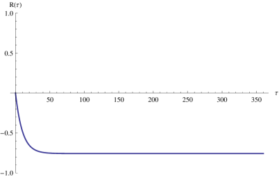
(b) $\theta_{1}=-0.075,\theta_{2}=0$

(c) $\theta_{1}=0,\theta_{2}=0.75$

(d) $\theta_{1}=0,\theta_{2}=-0.75$

Figure 1. Risk premium profiles when $L$ is a compound Poisson process with exponentially distributed jumps. Esscher transform: case $\bar{\beta}=(0,0).$ Arithmetic spot price model

Remark 4.8.

The previous Lemma shows that the risk premium $R_{a,Q}^{F}(t,\tau)$ vanishes with rate given by equation $\left(\ref{Equ_DRiskprem_Zero_Arithmetic}\right)$ at the short end of the forward curve, when $\tau$ converges to zero, and approaches the value given in equation $(\ref{Equ_RPremium_Infinity_Arithmetic})$ at long end of the forward curve, when $\tau$ tends to infinity. It follows that the sign of $R_{a,Q}^{F}(t,\tau)$ in the short end of the forward curve will be positive if $\left(\ref{Equ_DRiskprem_Zero_Arithmetic}\right)$ is positive and negative if $\left(\ref{Equ_DRiskprem_Zero_Arithmetic}\right)$ is negative. Hence, a sufficient condition to obtain the empirically observed risk premium profiles (with positive values in the short end and negative values in the long end of the forward curve) is to choose the values of the parameters $\bar{\theta}\in\bar{D}_{L}$ and $\bar{\beta}\in[0,1]^{2}$ such that the following two conditions are simultaneously satisfied

$$\frac{\theta_{1}}{\alpha_{X}(1-\beta_{1})}+\frac{\kappa_{L}^{\prime}(\theta_{2})-\kappa_{L}^{\prime}(0)}{\alpha_{Y}(1-\beta_{2})}+\frac{\kappa_{L}^{\prime}(0)}{\alpha_{Y}}\frac{\beta_{2}}{1-\beta_{2}} <0,$$

$$X(t)\alpha_{X}\beta_{1}+Y(t)\alpha_{Y}\beta_{2}+\theta_{1}+\kappa_{L}^{\prime}(\theta_{2})-\kappa_{L}^{\prime}(0) >0.$$

We also recall here that, according to Remark 2.2, $\kappa^{\prime}(\theta)$ is positive, increasing function, so the sign of $\kappa_{L}^{\prime}(\theta_{2})-\kappa_{L}^{\prime}(0)$ is equal to the sign of $\theta_{2}.$ Moreover, it is easy to see that

$$-\kappa_{L}^{\prime}(0)<\kappa_{L}^{\prime}(\theta_{2})-\kappa_{L}^{\prime}(0)<\kappa_{L}^{\prime}(\Theta_{L}/2)-\kappa_{L}^{\prime}(0)<\infty.$$

• Changing the level of mean reversion (Esscher transform), $\bar{\beta}=(0,0):$ Setting $\bar{\beta}=(0,0),$ the probability measure $Q$ only changes the level of mean reversion (which is assumed to be zero under the historical measure $P$). On the other hand, the risk premium is deterministic and cannot change with changing market conditions. From equation $\left(\ref{Equ_RPA_Esscher}\right),$ we get that if we set $\theta_{2}=0,$ which means that we just change the level of the regular factor $X,$ the sign of $R_{a,Q}^{F}(t,\tau)$ is the same for any time to maturity $\tau$ and it is equal to the sign of $\theta_{1},$ see Figures 1(a) and 1(b). The situation is similar if we set $\theta_{1}=0,$ then the sign of $R_{a,Q}^{F}(t,\tau)$ is constant over the time to maturity $\tau$ end equal to the sign of $\kappa_{L}^{\prime}(\theta_{2})-\kappa_{L}^{\prime}(0),$ that is to the sign of $\theta_{2},$ see Figures 1(c) and 1(d).

  

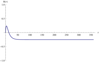
  (a) $\theta_{1}=-0.1,\theta_{2}=0.95$

  

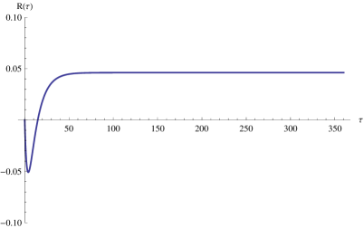
  (b) $\theta_{1}=0.02,\theta_{2}=-0.95$

  

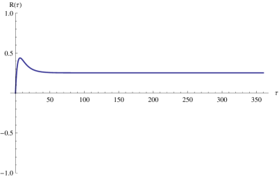
  (c) $\theta_{1}=-0.05,\theta_{2}=0.95$

  

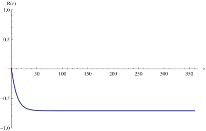
  (d) $\theta_{1}=-0.075,\theta_{2}=0.15$

  Figure 2. Risk premium profiles when $L$ is a compound Poisson process with exponentially distributed jumps. Esscher transform: case $\bar{\beta}=(0,0).$ Arithmetic spot price model

  When both $\theta_{1}$ and $\theta_{2}$ are different from zero the situation is more interesting, the sign of $R_{a,Q}^{F}(t,\tau)$ may change depending on the time to maturity. By Remark 4.8 it suffices to choose $\theta_{1}<0$ and $\theta_{2}>0$ satisfying

  $$\frac{\theta_{1}}{\alpha_{X}}+\frac{\kappa_{L}^{\prime}(\theta_{2})-\kappa_{L}^{\prime}(0)}{\alpha_{Y}} <0,$$ (4.10)

  $$\theta_{1}+\kappa_{L}^{\prime}(\theta_{2})-\kappa_{L}^{\prime}(0) >0,$$ (4.11)

  (these exist because $\alpha_{X}<\alpha_{Y}$ and $\kappa_{L}^{\prime}(\theta)$ is increasing) to get that $R_{a,Q}^{F}(t,\tau)>0$ for $\tau$ close to zero and $R_{a,Q}^{F}(t,\tau)<0$ for $\tau$ large enough, see Figure 2(a). This corresponds to the situation of a premium induced from consumers’ hedging pressure on short-term contracts and long term hedging of producers. We can also choose values for $\theta_{1}>0$ and $\theta_{2}<0$ such that equations 4.10 and 4.11 are satisfied but with inverted inequalities. In this way, we can get that $R_{a,Q}^{F}(t,\tau)<0$ for $\tau$ close to zero and $R_{a,Q}^{F}(t,\tau)>0$ for $\tau$ large enough, see Figure 2(b). Risk premium profiles with constant sign can also be generated, see Figures 2(c) and 2(d).

• Changing the speed of mean reversion, $\bar{\theta}=(0,0):$ Setting $\bar{\theta}=(0,0),$ the probability measure $Q$ only changes speed of mean reversion. Note that in this case the risk premium is stochastic and it changes with market conditions. By Lemma 4.7 we have that the risk premium is given by

  $$R_{a,Q}^{F}(t,\tau) =X(t)e^{-\alpha_{X}\tau}(e^{\alpha_{X}\beta_{1}\tau}-1)+Y(t)e^{-\alpha_{Y}\tau}(e^{\alpha_{Y}\beta_{2}\tau}-1)$$

  $$+\frac{\kappa_{L}^{\prime}(0)}{\alpha_{Y}}\Lambda(\alpha_{Y}\tau,1-\beta_{2}),$$

  and

  $$\lim_{\tau\rightarrow\infty}R_{a,Q}^{F}(t,\tau) =\frac{\kappa_{L}^{\prime}(0)}{\alpha_{Y}}\frac{\beta_{2}}{1-\beta_{2}}\geq 0,$$

  $$\lim_{\tau\rightarrow 0}\frac{\partial}{\partial\tau}R_{a,Q}^{F}(t,\tau) =X(t)\alpha_{X}\beta_{1}+Y(t)\alpha_{Y}\beta_{2}.$$

  Hence the risk premium will approach to a non negative value in the long end of the market. In the short end, it can be both positive or negative and stochastically varying with $X(t)$ and $Y(t),$ but $Y(t)$ will always contribute to a positive sign. Actually, as the function $\Lambda(x,y)$ is non-negative and $\kappa_{L}^{\prime}(0)$ is strictly positive, the only negative contribution to $R_{a,Q}^{F}(t,\tau)$ comes from the term due to the base component $X$. Hence, if $\beta_{1}=0$ or $X(t)\geq 0,$ then $R_{a,Q}^{F}(t,\tau)$ will be positive for all times to maturity. Some of the possible risk profiles that can be obtained are plotted in Figure 3.

  

  (a) $\beta_{1}=0.25,\beta_{2}=0.75,X(t)=2.5,Y(t)=2.5$

  

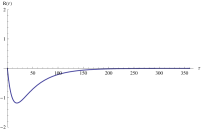
  (b) $\beta_{1}=0.75,\beta_{2}=0,X(t)=-2.5,Y(t)=2.5$

  

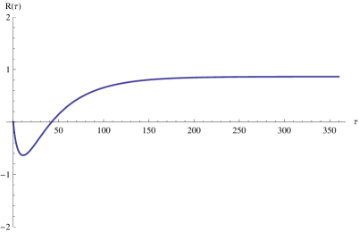
  (c) $\beta_{1}=0.75,\beta_{2}=0.75,X(t)=-2.5,Y(t)=0$

  

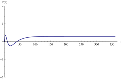
  (d) $\beta_{1}=0.5,\beta_{2}=0.5,X(t)=-2.5,Y(t)=2.5$

  Figure 3. Risk premium profiles when $L$ is a compound Poisson process with exponentially distributed jumps. Case $\bar{\theta}=(0,0).$ Arithmetic spot price model

  

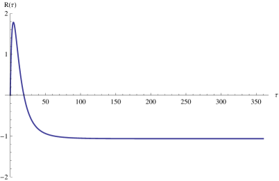
  (a) $\beta_{1}=0,\beta_{2}=0.88,\theta_{1}=-0.5,\theta_{2}=0.5,X(t)=\mathbb{R},Y(t)=5$

  Figure 4. Risk premium profiles when $L$ is a compound Poisson process with exponentially distributed jumps. Arithmetic spot price model

• Changing the level and speed of mean reversion simultaneously: The general case is quite complex to analyse. As we are more interested in how the change of measure $Q$ influence the component $Y(t)$, responsible for the spikes in the prices, we are going to assume that $\beta_{1}=0.$ This means that $Q$ may change the level of mean reversion of the regular component $X(t),$ but not the speed at which this component reverts to that level. The first implication of this assumption is that the possible stochastic component in $R_{a,Q}^{F}(t,\tau)$ due to $X(t)$ vanish. This simplifies the analysis as this term could be positive or negative. By Lemma 4.7 we get that

  $$R_{a,Q}^{F}(t,\tau) =Y(t)e^{-\alpha_{Y}\tau}(e^{\alpha_{Y}\beta_{2}\tau}-1)+\frac{\theta_{1}}{\alpha_{X}}(1-e^{-\alpha_{X}\tau})$$

  $$+\frac{\kappa_{L}^{\prime}(\theta_{2})}{\alpha_{Y}(1-\beta_{2})}(1-e^{-\alpha_{Y}(1-\beta_{2})\tau})-\frac{\kappa_{L}^{\prime}(0)}{\alpha_{Y}}(1-e^{-\alpha_{Y}\tau}).$$

  and

  $$\lim_{\tau\rightarrow\infty}R_{a,Q}^{F}(t,\tau) =\frac{\theta_{1}}{\alpha_{X}}+\frac{\kappa_{L}^{\prime}(\theta_{2})-\kappa_{L}^{\prime}(0)}{\alpha_{Y}(1-\beta_{2})}+\frac{\kappa_{L}^{\prime}(0)}{\alpha_{Y}}\frac{\beta_{2}}{1-\beta_{2}},$$ (4.12)

  $$\lim_{\tau\rightarrow 0}\frac{\partial}{\partial\tau}R_{a,Q}^{F}(t,\tau) =Y(t)\alpha_{Y}\beta_{2}+\theta_{1}+\kappa_{L}^{\prime}(\theta_{2})-\kappa_{L}^{\prime}(0).$$ (4.13)

  Note that we can make equation $\left(\ref{Equ_RPA_General_1}\right)$ negative by simply choosing $\theta_{1}$

  $$\theta_{1}<-\frac{\alpha_{X}}{\alpha_{Y}(1-\beta_{2})}\left(\kappa_{L}^{\prime}(\theta_{2})-\kappa_{L}^{\prime}(0)+\beta_{2}\kappa_{L}^{\prime}(0)\right).$$ (4.14)

  On the other hand, to make equation $(\ref{Equ_RPA_General_2})$ positive, we have to choose $\theta_{1}$ satisfying

  $$\theta_{1}>-(\kappa_{L}^{\prime}(\theta_{2})-\kappa_{L}^{\prime}(0))-Y(t)\alpha_{Y}\beta_{2}.$$ (4.15)

  Equations $\left(\ref{Equ_RPA_General_3}\right)$ and $\left(\ref{Equ_RPA_General_4}\right)$ are compatible if the following inequality is satisfied

  $$\kappa_{L}^{\prime}(\theta_{2})-\kappa_{L}^{\prime}(0)+Y(t)\alpha_{Y}\beta_{2}>\frac{\alpha_{X}}{\alpha_{Y}(1-\beta_{2})}\left(\kappa_{L}^{\prime}(\theta_{2})-\kappa_{L}^{\prime}(0)+\beta_{2}\kappa_{L}^{\prime}(0)\right).$$ (4.16)

  For any $\theta_{2}>0,$ which yields $\kappa_{L}^{\prime}(\theta_{2})-\kappa_{L}^{\prime}(0)>0$ (and $\theta_{1}<0$), we have that there exists $\beta_{2}^{\ast}\in(0,1)$ such that if $\beta_{2}<\beta_{2}^{\ast}$ equation $\left(\ref{Equ_RPA_General_5}\right)$ is satisfied. Actually, the larger the value of $Y(t),$ the larger the value of $\beta_{2}^{\ast}$. If $Y(t)$ is close to $\kappa_{L}^{\prime}(0)/\alpha_{Y},$ then $\beta_{2}^{\ast}$ is close to $(\alpha_{Y}-\alpha_{X})/\alpha_{Y}.$ This just says that if the speed of mean reversion of the spikes component is large (in absolute value and relatively to the speed of mean reversion of the base component) one can choose $\beta_{2}$ close to one. Even in the case that $Y(t)=0$, equation $\left(\ref{Equ_RPA_General_5}\right)$ is satisfied by choosing $\beta_{2}$ small enough. To sum up, we can create a measure $Q$ that can have a positive premium in the short end of the forward market due to sudden positive spikes in the price (that is, $Y$ increases), whereas in the long end of the market these spikes are not influential and we have a negative premium, see Figure 4.

4.2. Geometric spot price model

We assume in this section that the spot price $S(t)$ follows the geometric model $\eqref{Equ_Geom_Model}$ for $0\leq t\leq T^{\ast}$, $T^{\ast}>0$ and with the maturity of the forward contract being $0<T<T^{\ast}$. In our setting, the geometric model is harder to deal with than the arithmetic one. The results obtained are fair less explicit and some additional integrability conditions on $L$ are required. A first, natural, additional assumption on $L$ is that the constant $\Theta_{L}$ appearing in Assumption 1 to be bigger than $1.$ This condition is reasonable to expect because it just states that $\mathbb{E}[e^{L(t)}]<\infty,$ for all $t\in\mathbb{R}$ , and if we want $\mathbb{E}[e^{Y(t)}]$ to be finite it seems a minimal assumption. Note, however that this is not entirely obvious because the process $Y$ has a mean reversion structure that $L$ does not have. On the other hand, the complex probabilistic structure of the spike factor $Y$ under the new probability measure $Q,$ makes the computations much more difficult. Still, it is possible to compute the risk premium analytically in some cases. In general, one has to rely on numerical techniques.

In what follows, we shall compute the conditional expectations involved under $Q$ (note that $Q=P,$ when $\theta_{1}=\theta_{2}=\beta_{1}=\beta_{2}=0$). First, we show that the problem can be reduced to the study of the spike component $Y.$ Due to the independence of $X$ and $Y,$ we have that

$$\mathbb{E}_{Q}[S(T)] =\Lambda_{g}(T)\mathbb{E}_{Q}[\exp(X(T)+Y(T))]$$

$$=\Lambda_{g}(T)\mathbb{E}_{Q}[\exp(X(T))]\mathbb{E}_{Q}[\exp(Y(T))],$$

which is finite if and only $\mathbb{E}_{Q}[\exp(X(T))]<\infty$ and $\mathbb{E}_{Q}[\exp(Y(T))]<\infty.$ As $X(T)$ is a Gaussian random variable it has finite exponential moments. To determine whether $\mathbb{E}_{Q}[\exp(Y(T))]$ is finite or not is not as straightforward. Let us assume, for now, that it is finite. Then, it makes sense to compute the following conditional expectation

$$\mathbb{E}_{Q}[S(T)|\mathcal{F}_{t}] =\Lambda_{g}(T)\mathbb{E}_{Q}[\exp(X(T)+Y(T))|\mathcal{F}_{t}]$$

$$=\Lambda_{g}(T)\mathbb{E}_{Q}[\mathbb{E}_{Q}[\exp(X(T))|\mathcal{F}_{t}\vee\sigma(\{Y(t)\}_{0\leq t\leq T})]\exp(Y(T))|\mathcal{F}_{t}].$$

Using $\left(\ref{Equ_X_Explicit_Q}\right)$, the fact that $X$ is independent of $\sigma(\{Y(t)\}_{0\leq t\leq T})$ and basic properties of the conditional expectation we get that

$$\mathbb{E}_{Q}[\exp(X(T))|\mathcal{F}_{t}\vee\sigma(\{Y(t)\}_{0\leq t\leq T})]$$

$$=\exp\left(X(t)e^{-\alpha_{X}(1-\beta_{1})(T-t)}+\frac{\mu_{X}+\theta_{1}}{\alpha_{X}(1-\beta_{1})}(1-e^{-\alpha_{X}(1-\beta_{1})(T-t)})\right)$$

$$\qquad\times\mathbb{E}_{Q}[\exp\left(\sigma_{X}\int_{t}^{T}e^{-\alpha_{X}(1-\beta_{1})(T-s)}dW_{Q}(s)\right)]$$

$$=\exp\left(X(t)e^{-\alpha_{X}(1-\beta_{1})(T-t)}+\frac{\mu_{X}+\theta_{1}}{\alpha_{X}(1-\beta_{1})}(1-e^{-\alpha_{X}(1-\beta_{1})(T-t)})\right)$$

$$\qquad\times\exp\left(\frac{\sigma_{X}^{2}}{4\alpha_{X}(1-\beta_{1})}(1-e^{-2\alpha_{X}(1-\beta_{1})(T-t)})\right).$$

Hence, we have reduced the problem to the study of $\mathbb{E}_{Q}[\exp(Y(T))|\mathcal{F}_{t}].$

Let us start with the Esscher case $Q=Q_{\theta_{2},\beta_{2}}$ with $\theta_{2}\in D_{L}$ and $\beta_{2}=0.$ We have that

$$\mathbb{E}_{Q}[\exp(Y(T))] =\exp\left\{Y(0)e^{-\alpha_{Y}T}+\frac{\mu_{Y}+\kappa_{L}^{\prime}(\theta_{2})}{\alpha_{Y}}(1-e^{-\alpha_{Y}T})\right\}$$

$$\qquad\times\mathbb{E}_{Q}[\exp\left(\int_{0}^{T}\int_{0}^{\infty}ze^{-\alpha_{Y}(T-s)}\tilde{N}_{Q}^{L}(ds,dz)\right)]$$

$$=\exp\left\{Y(0)e^{-\alpha_{Y}T}+\frac{\mu_{Y}}{\alpha_{Y}}(1-e^{-\alpha_{Y}T})\right\}$$

$$\qquad\times\mathbb{E}_{Q}[\exp\left(\int_{0}^{T}\int_{0}^{\infty}ze^{-\alpha_{Y}(T-s)}N_{Q}^{L}(ds,dz)\right)]$$

$$=\exp\left\{Y(0)e^{-\alpha_{Y}T}+\frac{\mu_{Y}}{\alpha_{Y}}(1-e^{-\alpha_{Y}T})\right\}$$

$$\qquad\times\exp\left\{\int_{0}^{T}\int_{0}^{\infty}(e^{ze^{-\alpha_{Y}(T-s)}}-1)e^{\theta_{2}z}\ell(dz)ds\right\},$$

where we have used that the compensator of $L$ under $Q$ is $v_{Q}^{L}(ds,dz)=e^{\theta_{2}z}\ell(dz)ds$ (note that $e^{\theta_{2}z}\ell(dz)$ is a Lévy measure) and Proposition 3.6 in Cont and Tankov [8]. Of course, the previous result holds as long as the integral in the exponential is finite. A sufficient condition for the integrability of $\exp(Y(T))$ follows from

$$\int_{0}^{T}\int_{0}^{\infty}(e^{ze^{-\alpha_{Y}(T-s)}}-1)e^{\theta_{2}z}\ell(dz)ds$$

$$\qquad=\int_{0}^{T}\int_{0}^{\infty}ze^{-\alpha_{Y}(T-s)}\left(\int_{0}^{1}e^{\lambda ze^{-\alpha_{Y}(T-s)}}d\lambda\right)e^{\theta_{2}z}\ell(dz)ds$$

$$\qquad\leq\int_{0}^{T}\int_{0}^{\infty}ze^{-\alpha_{Y}(T-s)}e^{z\left(\theta_{2}+e^{-\alpha_{Y}(T-s)}\right)}\ell(dz)ds\leq T\kappa_{L}^{\prime}(\theta_{2}+1).$$

As $\theta_{2}\in D_{L},$ to have $\kappa_{L}^{\prime}(\theta_{2}+1)<\infty$ yields the condition

$$\theta_{2}\in D_{L}^{g}\triangleq D_{L}\cap(-\infty,\Theta_{L}-1)=(-\infty,(\Theta_{L}-1)\wedge(\Theta_{L}/2)).$$

Note that for $\theta_{2}\in D_{L}^{g}$ to be strictly positive and, therefore, include the case $Q=P$, we need to have $\Theta_{L}>1.$ This, of course, is a restriction on the structure of the jumps. For instance, if $L$ is a compound Poisson process with exponentially distributed jump sizes, Example 3.2 (Case 2), we have that the jump sizes must have a mean less than one. Note also that, if $\Theta_{L}>2$ then $D_{L}^{g}=D_{L}.$

Using expression $\left(\ref{Equ_Y_Explicit_Q}\right)$ and repeating the previous arguments we obtain

$$\mathbb{E}_{Q}[\exp(Y(T))|\mathcal{F}_{t}] =\exp\left\{Y(t)e^{-\alpha_{Y}(T-t)}+\frac{\mu_{Y}}{\alpha_{Y}}(1-e^{-\alpha_{Y}(T-t)})\right\}$$

$$\qquad\times\exp\left\{\int_{0}^{T-t}\int_{0}^{\infty}(e^{ze^{-\alpha_{Y}s}}-1)e^{\theta_{2}z}\ell(dz)ds\right\}.$$

Hence we have proved the following result:

Proposition 4.9.

In the Esscher case for the spike component $Y$, i.e., $\theta_{2}\in D_{L}^{g},$ $\beta_{2}=0$, and assuming $\Theta_{L}>1,$ the forward price $F_{Q}(t,T)$ in the geometric spot model $\left(\ref{Equ_Geom_Model}\right)$ is given by

$$F_{Q}(t,T) =\Lambda_{g}(T)\exp\left(X(t)e^{-\alpha_{X}(1-\beta_{1})(T-t)}+Y(t)e^{-\alpha_{Y}(T-t)}\right)$$

$$\qquad\times\exp\left(\frac{\mu_{X}+\theta_{1}}{\alpha_{X}(1-\beta_{1})}(1-e^{-\alpha_{X}(1-\beta_{1})(T-t)})+\frac{\mu_{Y}}{\alpha_{Y}}(1-e^{-\alpha_{Y}(T-t)})\right)$$

$$\qquad\times\exp\left(\frac{\sigma_{X}^{2}}{4\alpha_{X}(1-\beta_{1})}(1-e^{-2\alpha_{X}(1-\beta_{1})(T-t)})+\int_{0}^{T-t}\int_{0}^{\infty}(e^{ze^{-\alpha_{Y}s}}-1)e^{\theta_{2}z}\ell(dz)ds\right).$$

and the risk premium for the forward price $R_{g,Q}^{F}(t,T)$ is given by

$$R_{g,Q}^{F}(t,T) =\mathbb{E}_{P}[S(T)|\mathcal{F}_{t}]\{\exp(R_{a,Q}^{F}(t,T))$$

$$\qquad\times\exp\left(\frac{\sigma_{X}^{2}}{4\alpha_{X}(1-\beta_{1})}(1-e^{-2\alpha_{X}(1-\beta_{1})(T-t)}-\frac{\sigma_{X}^{2}}{4\alpha_{X}}(1-e^{-2\alpha_{X}(T-t)}\right)$$

$$\qquad\times\exp\left(-\frac{\kappa_{L}^{\prime}(\theta_{2})-\kappa_{L}^{\prime}(0)}{\alpha_{Y}}(1-e^{-\alpha_{Y}(T-t)})\right)$$

$$\qquad\times\exp\left(\int_{0}^{T-t}\int_{0}^{\infty}(e^{ze^{-\alpha_{Y}s}}-1)(e^{\theta_{2}z}-1)\ell(dz)ds\right)-1\},$$

where $R_{a,Q}^{F}(t,T)$ is also understood under the assumption $\beta_{2}=0.$

Corollary 4.10.

Setting $\theta_{2}=0$ in Proposition 4.9 we get

$$\mathbb{E}_{P}[S(T)|\mathcal{F}_{t}] =\Lambda_{g}(T)\exp\left(X(t)e^{-\alpha_{X}(T-t)}+Y(t)e^{-\alpha_{Y}(T-t)}\right)$$

$$\qquad\times\exp\left(\frac{\mu_{X}}{\alpha_{X}}(1-e^{-\alpha_{X}(T-t)})+\frac{\mu_{Y}}{\alpha_{Y}}(1-e^{-\alpha_{Y}(T-t)})\right)$$

$$\qquad\times\exp\left(\frac{\sigma_{X}^{2}}{4\alpha_{X}}(1-e^{-2\alpha_{X}(1-\beta_{1})(T-t)})+\int_{0}^{T-t}\int_{0}^{\infty}(e^{ze^{-\alpha_{Y}s}}-1)\ell(dz)ds\right).$$

The previous result is as far as one can go using ”basic” martingale techniques. In the general case, in order to find conditions under which $\mathbb{E}_{Q}[\exp(Y(T))]<\infty$, and also to compute $\mathbb{E}_{Q}[\exp(Y(T))|\mathcal{F}_{t}],$ it is convenient to look at $Y$ as an affine $Q$-semimartingale process with state space $\mathbb{R}_{+}$. In the sequel we follow the notation in Kallsen and Muhle-Karbe [15], but taking into account that in our case the Lévy characteristics do not depend on the time parameter. The Lévy-Kintchine triplets of $Y$ are

$$(\beta_{0}^{1},\gamma_{0}^{11},\varphi_{0}(dz)) =(\mu_{Y}+\kappa_{L}^{\prime}(\theta_{2}),0,\boldsymbol{1}_{(0,\infty)}e^{\theta_{2}z}\ell(dz))$$

$$(\beta_{1}^{1},\gamma_{1}^{11},\varphi_{1}(dz)) =(-\alpha_{Y}(1-\beta_{2}),0,\frac{\alpha_{Y}\beta_{2}}{\kappa_{L}^{\prime\prime}(\theta_{2})}\boldsymbol{1}_{(0,\infty)}ze^{\theta_{2}z}\ell(dz)),$$

which, according to Definition 2.4 in Kallsen and Muhle-Karbe [15], are (strongly) admissible. Note that, as the triplets do not depend on $t,$ we can choose any truncation function. Moreover, as $Y$ is a special $Q$-semimartingale, we choose the (pseudo) truncation function $h(x)=x.$ Associated to the previous Lévy-Kintchine triplets we have the following Lévy exponents

$$\Lambda_{0}^{\theta_{2},\beta_{2}}(u) =\left(\mu_{Y}+\kappa_{L}^{\prime}(\theta_{2})\right)u+\int_{0}^{\infty}(e^{uz}-1-uz)e^{\theta_{2}z}\ell(dz)$$

$$=\mu_{Y}u+\int_{0}^{\infty}(e^{uz}-1)e^{\theta_{2}z}\ell(dz)$$

$$=\mu_{Y}u+\kappa_{L}(u+\theta_{2})-\kappa_{L}(\theta_{2}),$$

$$\Lambda_{1}^{\theta_{2},\beta_{2}}(u) =-\alpha_{Y}(1-\beta_{2})u+\frac{\alpha_{Y}\beta_{2}}{\kappa_{L}^{\prime\prime}(\theta_{2})}\int_{0}^{\infty}(e^{uz}-1-uz)ze^{\theta_{2}z}\ell(dz)$$

$$=-\alpha_{Y}u+\frac{\alpha_{Y}\beta_{2}}{\kappa_{L}^{\prime\prime}(\theta_{2})}\int_{0}^{\infty}(e^{uz}-1)ze^{\theta_{2}z}\ell(dz)$$

$$=-\alpha_{Y}u+\frac{\alpha_{Y}\beta_{2}}{\kappa_{L}^{\prime\prime}(\theta_{2})}\left(\kappa_{L}^{\prime}(u+\theta_{2})-\kappa_{L}^{\prime}(\theta_{2})\right).$$

We have the following result.

Theorem 4.11.

Let $\bar{\beta}\in[0,1]^{2},\bar{\theta}\in\bar{D}_{L}^{g}\triangleq\mathbb{R}\times D_{L}^{g}$. Assume $\Theta_{L}>1,$ that $\Psi_{\theta_{2},\beta_{2}}^{0},\Psi_{\theta_{2},\beta_{2}}^{1}\in C^{1}([0,T],\mathbb{R})$ satisfy the ODE

$$\begin{array}[c]{ccc}\frac{d}{dt}\Psi_{\theta_{2},\beta_{2}}^{1}(t)=\Lambda_{1}^{\theta_{2},\beta_{2}}(\Psi_{\theta_{2},\beta_{2}}^{1}(t)),&&\Psi_{\theta_{2},\beta_{2}}^{1}(0)=1,\\ \frac{d}{dt}\Psi_{\theta_{2},\beta_{2}}^{0}(t)=\Lambda_{0}^{\theta_{2},\beta_{2}}(\Psi_{\theta_{2},\beta_{2}}^{1}(t)),&&\Psi_{\theta_{2},\beta_{2}}^{0}(0)=0,\end{array}$$ (4.17)

and that the integrability condition

$$\kappa_{L}^{\prime\prime}(\theta_{2}+\sup_{t\in[0,T]}\Psi_{\theta_{2},\beta_{2}}^{1}(t))=\int_{0}^{\infty}z^{2}\exp\{(\theta_{2}+\sup_{t\in[0,T]}\Psi_{\theta_{2},\beta_{2}}^{1}(t))z\}\ell(dz)<\infty,$$ (4.18)

holds. Then, we have that the forward price $F_{Q}(t,T)$ in the geometric spot model $\left(\ref{Equ_Geom_Model}\right)$ is given by

$$F_{Q}(t,T) =\Lambda_{g}(T)\exp\left(X(t)e^{-\alpha_{X}(1-\beta_{1})(T-t)}+Y(t)\Psi_{\theta_{2},\beta_{2}}^{1}(T-t)+\Psi_{\theta_{2},\beta_{2}}^{0}(T-t)\right)$$

$$\qquad\times\exp\left(\frac{\mu_{X}+\theta_{1}}{\alpha_{X}(1-\beta_{1})}(1-e^{-\alpha_{X}(1-\beta_{1})(T-t)})+\frac{\sigma_{X}^{2}}{4\alpha_{X}(1-\beta_{1})}(1-e^{-2\alpha_{X}(1-\beta_{1})(T-t)})\right),$$

and the risk premium for the forward price $R_{g,Q}^{F}(t,T)$ is given by

$$R_{g,Q}^{F}(t,T) =\mathbb{E}_{P}[S(T)|\mathcal{F}_{t}]\{\exp(X(t)e^{-\alpha_{X}(T-t)}(e^{\alpha_{X}\beta_{1}(T-t)}-1))$$

$$\qquad\times\exp(Y(t)(\Psi_{\theta_{2},\beta_{2}}^{1}(T-t)-e^{-\alpha_{Y}(T-t)}))$$

$$\qquad\times\exp\left(\frac{\mu_{X}+\theta_{1}}{\alpha_{X}(1-\beta_{1})}(1-e^{-\alpha_{X}(1-\beta_{1})(T-t)})-\frac{\mu_{X}}{\alpha_{X}}(1-e^{-\alpha_{X}(T-t)})\right)$$

$$\qquad\times\exp\left(\frac{\sigma_{X}^{2}}{4\alpha_{X}(1-\beta_{1})}(1-e^{-2\alpha_{X}(1-\beta_{1})(T-t)})-\frac{\sigma_{X}^{2}}{4\alpha_{X}}(1-e^{-2\alpha_{X}(T-t)})\right)$$

$$\qquad\times\exp\left(\Psi_{\theta_{2},\beta_{2}}^{0}(T-t)-\frac{\mu_{Y}}{\alpha_{Y}}(1-e^{-\alpha_{Y}(T-t)})-\int_{0}^{T-t}\int_{0}^{\infty}(e^{ze^{-\alpha_{Y}s}}-1)\ell(dz)ds\right)-1\}.$$

Proof.

We apply Theorem 5.1 in Kallsen and Muhle-Karbe [15]. Note that making the change of variable $t\rightarrow T-t$ the ODE $\left(\ref{Equ_ODE}\right)$ is reduced to the one appearing in items 2. and 3. of Theorem 5.1. The integrability assumption $\left(\ref{Equ_Integrability_ODE}\right)$ implies conditions 1. and 5., in Theorem 5.1, and condition 4. is trivially satisfied because $Y(0)$ is deterministic. Hence, the conclusion of that theorem, with $p=1,$ holds and we get

$$\mathbb{E}_{Q}[\exp(Y(T))|\mathcal{F}_{t}]=\exp\left(Y(t)\Psi_{\theta_{2},\beta_{2}}^{1}(T-t)+\Psi_{\theta_{2},\beta_{2}}^{0}(T-t)\right),\quad t\in[0,T].$$ (4.19)

The result now follows easily. ∎

Remark 4.12.

Equation $\left(\ref{Equ_ODE}\right)$ is called a generalised Riccati equation in the literature. Note that the equation for $\Psi_{\theta_{2},\beta_{2}}^{0}(t)$ is trivially solved, once we know $\Psi_{\theta_{2},\beta_{2}}^{1}(t),$ by

$$\Psi_{\theta_{2},\beta_{2}}^{0}(t)=\int_{0}^{t}\Lambda_{0}^{\theta_{2},\beta_{2}}(\Psi_{\theta_{2},\beta_{2}}^{1}(s))ds.$$

Hence, the problem is really reduced to study the equation for $\Psi_{\theta_{2},\beta_{2}}^{1}(t).$

Remark 4.13.

The Esscher case can be obtained from Theorem 4.11, as $\Psi_{\theta_{2},0}^{1}(t)=e^{-\alpha_{Y}t}$ and

$$\Psi_{\theta_{2},0}^{0}(t)=\frac{\mu_{Y}}{\alpha_{Y}}(1-e^{-\alpha_{Y}t})+\int_{0}^{t}\int_{0}^{\infty}(e^{ze^{-\alpha_{Y}s}}-1)e^{\theta_{2}z}\ell(dz)ds,$$

solve

$$\begin{array}[c]{ccc}\frac{d}{dt}\Psi_{\theta_{2},0}^{1}(t)=-\alpha_{Y}\Psi_{\theta_{2},0}^{1}(t),&&\Psi_{\theta_{2},0}^{1}(0)=1,\\ \frac{d}{dt}\Psi_{\theta_{2},0}^{0}(t)=\mu_{Y}\Psi_{\theta_{2},0}^{1}(t)+\kappa_{L}(\Psi_{\theta_{2},0}^{1}(t)+\theta_{2})-\kappa_{L}(\theta_{2}),&&\Psi_{\theta_{2},0}^{0}(0)=0.\end{array}$$

As $\sup_{t\in[0,T]}\Psi_{\theta_{2},0}^{1}(t)=1,$ the integrability condition $\left(\ref{Equ_Integrability_ODE}\right)$ is satisfied because $\theta_{2}\in D_{L}^{g}.$

In general, one cannot find explicit solutions for the non-linear differential equation $\left(\ref{Equ_ODE}\right)$ in Theorem 4.11 and has to rely on numerical techniques. However, the main problem that we find is that the maximal domain of definition of $\Psi_{\theta_{2},\beta_{2}}^{0}$ and $\Psi_{\theta_{2},\beta_{2}}^{1}$ may be a proper subset of $[0,\infty),$ in particular when $\beta_{2}$ is close to $1$. As we are particularly interested in the solution of $\left(\ref{Equ_ODE}\right)$ for large $T$, we shall give a general sufficient criterion for global (defined for any $t>0$) existence and uniqueness of the solution of $\left(\ref{Equ_ODE}\right)$. The next theorem classifies the behaviour of the solutions of $\left(\ref{Equ_ODE}\right)$.

Theorem 4.14.

Assume that $\Theta_{L}>1.$ For any $\delta>0,$ the system of ODEs (4.17) with $\beta_{2}\in(0,1)$ and

$$\theta_{2}\in D_{L}^{g}(\delta)\triangleq(-\infty,(\Theta_{L}-1-\delta)\wedge(\Theta_{L}/2))$$

admits a unique local solution $\Psi_{\theta_{2},\beta_{2}}^{0}(t)$ and $\Psi_{\theta_{2},\beta_{2}}^{1}(t)$. In addition, let $u^{\ast}(\theta_{2},\beta_{2})$ be the unique strictly positive solution of the following equation

$$u=\frac{\beta_{2}}{\kappa_{L}^{\prime\prime}(\theta_{2})}\left(\kappa_{L}^{\prime}(u+\theta_{2})-\kappa_{L}^{\prime}(\theta_{2})\right).$$ (4.20)

The behaviour of $\Psi_{\theta_{2},\beta_{2}}^{0}(t)$ and $\Psi_{\theta_{2},\beta_{2}}^{1}(t)$ is characterised as follows:

1. If $u^{\ast}(\theta_{2},\beta_{2})>1,$ then $\Psi_{\theta_{2},\beta_{2}}^{0}(t)$ and $\Psi_{\theta_{2},\beta_{2}}^{1}(t)$ are globally defined, satisfy

   $$0<\Psi_{\theta_{2},\beta_{2}}^{1}(t)\leq 1,\qquad 0\leq\Psi_{\theta_{2},\beta_{2}}^{0}(t)\leq\int_{0}^{\infty}\Lambda_{0}^{\theta_{2},\beta_{2}}(\Psi_{\theta_{2},\beta_{2}}^{1}(s))ds<\infty,$$

   and

   $$\lim_{t\rightarrow\infty}\frac{1}{t}\log(\Psi_{\theta_{2},\beta_{2}}^{1}(t)) =-\alpha_{Y}(1-\beta_{2}),$$ (4.21)

   $$\lim_{t\rightarrow\infty}\Psi_{\theta_{2},\beta_{2}}^{0}(t) =\int_{0}^{\infty}\Lambda_{0}^{\theta_{2},\beta_{2}}(\Psi_{\theta_{2},\beta_{2}}^{1}(s))ds<\infty.$$ (4.22)

2. If $u^{\ast}(\theta_{2},\beta_{2})=1,$ then $\Psi_{\theta_{2},\beta_{2}}^{1}(t)\equiv 1$ and $\Psi_{\theta_{2},\beta_{2}}^{0}(t)=\{\mu_{Y}+\kappa_{L}(1+\theta_{2})-\kappa_{L}(\theta_{2})\}t.$

3. If $u^{\ast}(\theta_{2},\beta_{2})<1$, then the maximal domain of definition of $\Psi_{\theta_{2},\beta_{2}}^{0}(t)$ and $\Psi_{\theta_{2},\beta_{2}}^{1}(t)$ is $[0,t_{\infty}),$ where

   $$0<t_{\infty}=\int_{1}^{\Theta_{L}-\theta_{2}}(\Lambda_{1}^{\theta_{2},\beta_{2}}(u))^{-1}du<\infty.$$

   In addition,

   $$\lim_{t\uparrow t_{\infty}}\Psi_{\theta_{2},\beta_{2}}^{1}(t)=\Theta_{L}-\theta_{2},\quad\lim_{t\uparrow t_{\infty}}\Psi_{\theta_{2},\beta_{2}}^{0}(t)=\int_{0}^{t_{\infty}}\Lambda_{0}^{\theta_{2},\beta_{2}}(\Psi_{\theta_{2},\beta_{2}}^{1}(s))ds,$$

   where the previous integral is non negative and may be finite or infinite.

Proof.

We have to study the vector field

$$\Lambda_{1}^{\theta_{2},\beta_{2}}(u)=-\alpha_{Y}u+\frac{\alpha_{Y}\beta_{2}}{\kappa_{L}^{\prime\prime}(\theta_{2})}\int_{0}^{\infty}(e^{uz}-1)ze^{\theta_{2}z}\ell(dz),\quad\beta_{2}\in[0,1],\theta_{2}\in D_{L}^{g}.$$

Consider

$$\mathcal{D}(\Lambda_{1}^{\theta_{2},\beta_{2}})\triangleq\mathrm{int}(\{u\in\mathbb{R}:\Lambda_{1}^{\theta_{2},\beta_{2}}(u)<\infty\})=\mathrm{int}(\{u\in\mathbb{R}:\kappa_{L}^{\prime}(u+\theta_{2})<\infty\})=(-\infty,\Theta_{L}-\theta_{2}),$$

and, for any $\delta>0,$ define

$$\mathcal{D}_{\delta} \triangleq\mathrm{int}({\displaystyle\bigcap\limits_{\beta_{2}\in[0,1],\theta_{2}\in D_{L}^{g}(\delta)}}\mathcal{D}(\Lambda_{1}^{\theta_{2},\beta_{2}}))=(-\infty,\Theta_{L}-((\Theta_{L}-1-\delta)\wedge(\Theta_{L}/2)))$$

$$=(-\infty,(1+\delta)\vee(\Theta_{L}/2))).$$

On the other hand, for $u,v\in\mathcal{D}(\Lambda_{1}^{\theta_{2},\beta_{2}}),$ one has that

$$\left|\Lambda_{1}^{\theta_{2},\beta_{2}}(u)-\Lambda_{1}^{\theta_{2},\beta_{2}}(v)\right|\leq\alpha_{Y}\left|u-v\right|+\frac{\alpha_{Y}\beta_{2}}{\kappa_{L}^{\prime\prime}(\theta_{2})}\int_{0}^{\infty}\left|e^{uz}-e^{vz}\right|ze^{\theta_{2}z}\ell(dz),$$

and

$$\int_{0}^{\infty}\left|e^{uz}-e^{vz}\right|ze^{\theta_{2}z}\ell(dz)\leq|u-v|\int_{0}^{\infty}e^{(u\vee v+\theta_{2})z}z^{2}\ell(dz),$$

Moreover, note that

$$\mathrm{int}(\{u\in\mathbb{R}:\int_{0}^{\infty}z^{2}e^{(u+\theta_{2})z}\ell(dz)<\infty\})=(-\infty,\Theta_{L}-\theta_{2})=\mathcal{D}(\Lambda_{1}^{\theta_{2},\beta_{2}}).$$

Hence, the vector field $\Lambda_{1}^{\theta_{2},\beta_{2}}(u),\theta_{2}\in D_{L}^{g}(\delta),\beta_{2}\in[0,1]$ is well defined (i.e., finite) and locally Lipschitz in $\mathcal{D}_{\delta}.$ As the initial condition for $\Psi_{\theta_{2},\beta_{2}}^{1}(t)$ is $\Psi_{\theta_{2},\beta_{2}}^{1}(0)=1$, it is natural to require that $1\in\mathcal{D}_{\delta}$ and this is precisely the role of $\delta>0.$ Then, by Picard-Lindelöf Theorem, see Theorem 3.1, pag. 18, in Hale [12], we have local existence and uniqueness for $\Psi_{\theta_{2},\beta_{2}}^{1}(t)$ and $\Psi_{\theta_{2},\beta_{2}}^{1}(0)\in\mathcal{D}_{\delta}.$ In addition, we have that $0\in\mathcal{D}_{\delta}$ and, hence, we have local existence and uniqueness for solutions of $\Psi_{\theta_{2},\beta_{2}}^{1}(t)$ with $\Psi_{\theta_{2},\beta_{2}}^{1}(0)=0.$ As $\Lambda_{1}^{\theta_{2},\beta_{2}}(0)=0,$ we have that $\Psi_{\theta_{2},\beta_{2}}^{1}(t)\equiv 0$ is the unique global solution of equation $\left(\ref{Equ_ODE}\right)$ starting at 0. As a consequence, it is sufficient to study the vector field $\Lambda_{1}^{\theta_{2},\beta_{2}}(u)$ for $u\geq 0,$ because any solution of equation $\left(\ref{Equ_ODE}\right)$ with $\Psi_{\theta_{2},\beta_{2}}^{1}(0)=1$ cannot cross to the negative real line without contradicting the uniqueness result at $0.$ The unicity of $\Psi_{\theta_{2},\beta_{2}}^{0}(t)$ trivially follows from that of $\Psi_{\theta_{2},\beta_{2}}^{1}(t).$ The next step is to study the zeros of $\Lambda_{1}^{\theta_{2},\beta_{2}}(u),u\in\mathcal{D}_{\delta}\cap[0,\infty).$ We have to solve the non-linear equation

$$0=\Lambda_{1}^{\theta_{2},\beta_{2}}(u)=-\alpha_{Y}u+\frac{\alpha_{Y}\beta_{2}}{\kappa_{L}^{\prime\prime}(\theta_{2})}\left(\kappa_{L}^{\prime}(u+\theta_{2})-\kappa_{L}^{\prime}(\theta_{2})\right).$$ (4.23)

Note that equation $\left(\ref{Equ_VectorField_Lamb1}\right)$ has the trivial solution $u=0.$ As the first and second derivatives of $\Lambda_{1}^{\theta_{2},\beta_{2}}(u)$ are

$$\frac{d}{du}\Lambda_{1}^{\theta_{2},\beta_{2}}(u) =-\alpha_{Y}+\frac{\alpha_{Y}\beta_{2}}{\kappa_{L}^{\prime\prime}(\theta_{2})}\kappa_{L}^{\prime\prime}(u+\theta_{2}),$$

$$\frac{d^{2}}{du^{2}}\Lambda_{1}^{\theta_{2},\beta_{2}}(u) =\frac{\alpha_{Y}\beta_{2}}{\kappa_{L}^{\prime\prime}(\theta_{2})}\kappa_{L}^{(3)}(u+\theta_{2})>0,$$

we have that there exists a unique $0<u^{\ast}(\theta_{2},\beta_{2})<\Theta_{L}-\theta_{2}$ for $\theta_{2}\in D_{L}^{g}(\delta)$ and $\beta_{2}\in(0,1)$ such that equation $\left(\ref{Equ_VectorField_Lamb1}\right)$ is satisfied. Moreover $\Lambda_{1}^{\theta_{2},\beta_{2}}(u)<0$ for $u\in(0,u^{\ast}(\theta_{2},\beta_{2}))$ and $\Lambda_{1}^{\theta_{2},\beta_{2}}(u)>0$ for $(u^{\ast}(\theta_{2},\beta_{2}),\Theta_{L}-\theta_{2}).$ When $\beta_{2}\downarrow 0,u^{\ast}(\theta_{2},\beta_{2})$ converges to $\Theta_{L}-\theta_{2}.$ On the other hand, when $\beta_{2}\uparrow 1,u^{\ast}(\theta_{2},\beta_{2})$ converges to zero. Therefore, we have three possible cases to discuss

• Case $\boldsymbol{1}:$ If $u^{\ast}(\theta_{2},\beta_{2})>1,$ then $\Psi_{\theta_{2},\beta_{2}}^{1}(t)$ will monotonically converge to $0$ and, by uniqueness of solutions, it will take an infinite amount of time to reach $0.$ Hence, $\Psi_{\theta_{2},\beta_{2}}^{1}(t)$ will be a globally defined bounded solution. The exponential rate of convergence of $\Psi_{\theta_{2},\beta_{2}}^{1}(t)$ to zero, equation 4.21, follows by applying Hôpital’s rule to

  $$\lim_{t\rightarrow\infty}t^{-1}\log(\Psi_{\theta_{2},\beta_{2}}^{1}(t)) =\lim_{t\rightarrow\infty}\frac{\frac{d}{dt}\Psi_{\theta_{2},\beta_{2}}^{1}(t)}{\Psi_{\theta_{2},\beta_{2}}^{1}(t)}$$

  $$=\lim_{t\rightarrow\infty}\frac{\Lambda_{1}^{\theta_{2},\beta_{2}}(\Psi_{\theta_{2},\beta_{2}}^{1}(t))}{\Psi_{\theta_{2},\beta_{2}}^{1}(t)}$$

  $$=\lim_{t\rightarrow\infty}\frac{-\alpha_{Y}\Psi_{\theta_{2},\beta_{2}}^{1}(t)+\frac{\alpha_{Y}\beta_{2}}{\kappa_{L}^{\prime\prime}(\theta_{2})}\{\kappa_{L}^{\prime}(\Psi_{\theta_{2},\beta_{2}}^{1}(t)+\theta_{2})-\kappa_{L}^{\prime}(+\theta_{2})\}}{\Psi_{\theta_{2},\beta_{2}}^{1}(t)}$$

  $$=-\alpha_{Y}+\frac{\alpha_{Y}\beta_{2}}{\kappa_{L}^{\prime\prime}(\theta_{2})}\lim_{t\rightarrow\infty}\frac{\int_{0}^{1}\kappa_{L}^{\prime\prime}(\theta_{2}+\lambda\Psi_{\theta_{2},\beta_{2}}^{1}(t))d\lambda\Psi_{\theta_{2},\beta_{2}}^{1}(t)}{\Psi_{\theta_{2},\beta_{2}}^{1}(t)}$$

  $$=-\alpha_{Y}(1-\beta_{2}).$$

  It follows that $\Psi_{\theta_{2},\beta_{2}}^{0}(t)$ will be also globally defined and, as $\Lambda_{0}^{\theta_{2},\beta_{2}}(u)=\mu_{Y}u+\int_{0}^{1}\kappa_{L}^{\prime}(\theta_{2}+\lambda u)d\lambda>0$ for $u\in(0,1),$ by monotone convergence

  $$\lim_{t\rightarrow\infty}\Psi_{\theta_{2},\beta_{2}}^{0}(t)=\int_{0}^{\infty}\Lambda_{0}^{\theta_{2},\beta_{2}}(\Psi_{\theta_{2},\beta_{2}}^{1}(s))ds.$$

  To show that the previous integral is actually finite, it suffices to prove that $\Lambda_{0}^{\theta_{2},\beta_{2}}(\Psi_{\theta_{2},\beta_{2}}^{1}(t))$ converges to zero faster than $t^{-(1+\varepsilon)},$ for some $\varepsilon>0,$ when $t$ tends to infinity. We have that

  $$\Lambda_{0}^{\theta_{2},\beta_{2}}(\Psi_{\theta_{2},\beta_{2}}^{1}(t)) =\mu_{Y}\Psi_{\theta_{2},\beta_{2}}^{1}(t)+\kappa_{L}(\Psi_{\theta_{2},\beta_{2}}^{1}(t)+\theta_{2})-\kappa_{L}(\theta_{2})$$

  $$=\{\mu_{Y}+\int_{0}^{1}\kappa_{L}^{\prime}(\theta_{2}+\lambda\Psi_{\theta_{2},\beta_{2}}^{1}(t))d\lambda\}\Psi_{\theta_{2},\beta_{2}}^{1}(t),$$

  and

  $$\frac{d}{dt}\left(\Lambda_{0}^{\theta_{2},\beta_{2}}(\Psi_{\theta_{2},\beta_{2}}^{1}(t))\right) =\left.\frac{d}{du}\Lambda_{0}^{\theta_{2},\beta_{2}}(u)\right|_{u=\Psi_{\theta_{2},\beta_{2}}^{1}(t)}\frac{d}{dt}\Psi_{\theta_{2},\beta_{2}}^{1}(t)$$

  $$=\{\mu_{Y}+\kappa_{L}^{\prime}(\theta_{2}+\Psi_{\theta_{2},\beta_{2}}^{1}(t))\}$$

  $$\qquad\times\{-\alpha_{Y}\Psi_{\theta_{2},\beta_{2}}^{1}(t)+\frac{\alpha_{Y}\beta_{2}}{\kappa_{L}^{\prime\prime}(\theta_{2})}\left(\kappa_{L}^{\prime}(\Psi_{\theta_{2},\beta_{2}}^{1}(t)+\theta_{2})-\kappa_{L}^{\prime}(\theta_{2})\right)\}$$

  $$=\{\mu_{Y}+\kappa_{L}^{\prime}(\theta_{2}+\Psi_{\theta_{2},\beta_{2}}^{1}(t))\}$$

  $$\qquad\times\{-\alpha_{Y}+\frac{\alpha_{Y}\beta_{2}}{\kappa_{L}^{\prime\prime}(\theta_{2})}\int_{0}^{1}\kappa_{L}^{\prime\prime}(\theta_{2}+\lambda\Psi_{\theta_{2},\beta_{2}}^{1}(t))d\lambda\}\Psi_{\theta_{2},\beta_{2}}^{1}(t).$$

  By Hôpital’s rule and equation $\left(\ref{Equ_Exp_Psi1}\right)$

  $$\lim_{t\rightarrow\infty}t^{(1+\varepsilon)}\Lambda_{0}^{\theta_{2},\beta_{2}}(\Psi_{\theta_{2},\beta_{2}}^{1}(t)) =\lim_{t\rightarrow\infty}(1+\varepsilon)t^{\varepsilon}\left(\frac{-\frac{d}{dt}\Lambda_{0}^{\theta_{2},\beta_{2}}(\Psi_{\theta_{2},\beta_{2}}^{1}(t))}{\left(\Lambda_{0}^{\theta_{2},\beta_{2}}(\Psi_{\theta_{2},\beta_{2}}^{1}(t))\right)^{2}}\right)^{-1}$$

  $$=(1+\varepsilon)\frac{\mu_{Y}+\kappa_{L}^{\prime}(\theta_{2})}{\alpha_{Y}(1-\beta_{2})}\lim_{t\rightarrow\infty}t^{\varepsilon}\Psi_{\theta_{2},\beta_{2}}^{1}(t)=0,$$

  and we can conclude that equation $\left(\ref{Equ_Infinity_Psi0}\right)$ holds.

• Case $\boldsymbol{2}:$ If $u^{\ast}(\theta_{2},\beta_{2})=1,$ then $\Psi_{\theta_{2},\beta_{2}}^{1}(t)\equiv 1,$ will be the unique global solution and

  $$\Psi_{\theta_{2},\beta_{2}}^{0}(t)=\int_{0}^{t}\Lambda_{0}^{\theta_{2},\beta_{2}}(\Psi_{\theta_{2},\beta_{2}}^{1}(s))ds=\{\mu_{Y}+\kappa_{L}(1+\theta_{2})-\kappa_{L}(\theta_{2})\}t.$$

• Case $\boldsymbol{3}:$ If $u^{\ast}(\theta_{2},\beta_{2})<1,$ then $\Psi_{\theta_{2},\beta_{2}}^{1}(t)$ will increase monotonically to $\Theta_{L}-\theta_{2},$ because the vector field $\Lambda_{1}^{\theta_{2},\beta_{2}}$ is strictly positive in $[1,\Theta_{L}-\theta_{2})$. Separating variables an integrating the equation for $\Psi_{\theta_{2},\beta_{2}}^{1}(t)$ with $\Psi_{\theta_{2},\beta_{2}}^{1}(0)=1$ we get that the maximal domain of definition of $\Psi_{\theta_{2},\beta_{2}}^{1}(t)$ is $[0,t_{\infty})$ with

  $$t_{\infty}\triangleq\int_{1}^{\Theta_{L}-\theta_{2}}(\Lambda_{1}^{\theta_{2},\beta_{2}}(u))^{-1}du.$$

  To show that $t_{\infty}$ is actually finite we have to distinguish between the case $\Theta_{L}<\infty$ and $\Theta_{L}=\infty.$ If $\Theta_{L}<\infty,$ then $(\Lambda_{1}^{\theta_{2},\beta_{2}}(u))^{-1}$ is bounded in $[1,\Theta_{L}-\theta_{2})$ and the integral is obviously finite. If $\Theta_{L}=\infty$ we have to ensure that $(\Lambda_{1}^{\theta_{2},\beta_{2}}(u))^{-1}$ converges to zero fast enough when $u$ tends to infinity. Note that, by monotone convergence, one has that

  $$\lim_{\theta\rightarrow\infty}\kappa_{L}(\theta) =\int_{0}^{\infty}\lim_{\theta\rightarrow\infty}(e^{\theta z}-1)\ell(dz)=\infty,$$

  $$\lim_{\theta\rightarrow\infty}\kappa_{L}^{(n)}(\theta) =\int_{0}^{\infty}\lim_{\theta\rightarrow\infty}z^{n}e^{\theta z}\ell(dz)=\infty,\quad n\geq 1.$$

  For any $0<\varepsilon<1,$ we have that

  $$\lim_{u\rightarrow\infty}u^{-(1+\varepsilon)}\Lambda_{1}^{\theta_{2},\beta_{2}}(u) =\lim_{u\rightarrow\infty}u^{-(1+\varepsilon)}\{-\alpha_{Y}u+\frac{\alpha_{Y}\beta_{2}}{\kappa_{L}^{\prime\prime}(\theta_{2})}(\kappa_{L}^{\prime}(u+\theta_{2})-\kappa_{L}^{\prime}(\theta_{2}))\}$$

  $$=\frac{\alpha_{Y}\beta_{2}}{\kappa_{L}^{\prime\prime}(\theta_{2})}\lim_{u\rightarrow\infty}\frac{\kappa_{L}^{\prime}(u+\theta_{2})}{u^{(1+\varepsilon)}}=\frac{\alpha_{Y}\beta_{2}}{(1+\varepsilon)\kappa_{L}^{\prime\prime}(\theta_{2})}\lim_{u\rightarrow\infty}\frac{\kappa_{L}^{\prime\prime}(u+\theta_{2})}{u^{\varepsilon}}$$

  $$=\frac{\alpha_{Y}\beta_{2}}{(1+\varepsilon)\varepsilon\kappa_{L}^{\prime\prime}(\theta_{2})}\lim_{u\rightarrow\infty}u^{1-\varepsilon}\kappa_{L}^{(3)}(u+\theta_{2})=\infty,$$

  which yields that the integral defining $t_{\infty}$ is finite. According to Remark 4.12, we have that

  $$\lim_{t\rightarrow t_{\infty}}\Psi_{\theta_{2},\beta_{2}}^{0}(t)=\int_{0}^{t_{\infty}}\Lambda_{0}^{\theta_{2},\beta_{2}}(\Psi_{\theta_{2},\beta_{2}}^{1}(s))ds,$$ (4.24)

  which may be finite or infinite depending, of course, on how fast $\Lambda_{0}^{\theta_{2},\beta_{2}}(\Psi_{\theta_{2},\beta_{2}}^{1}(s))$ diverges to infinity when $s$ approaches to $t_{\infty}.$

∎

As it does not seem possible to give simple conditions for the finiteness (or not) of the integral $\left(\ref{EquIntegralPsi0}\right)$ and it is not relevant in the discussion to follow, we do not proceed further in the analysis.

Remark 4.15.

If $\beta_{2}=0,$ then $\Psi_{\theta_{2},0}^{1}(t)=e^{-\alpha_{Y}t}$ and

$$\Psi_{\theta_{2},0}^{0}(t) =\int_{0}^{t}\mu_{Y}e^{-\alpha_{Y}s}ds+\int_{0}^{t}\kappa_{L}(e^{-\alpha_{Y}s}+\theta_{2})-\kappa_{L}(\theta_{2})ds$$

$$=\frac{\mu_{Y}}{\alpha_{Y}}(1-e^{-\alpha_{Y}t})+\int_{0}^{t}\int_{0}^{\infty}(e^{ze^{-\alpha_{Y}s}}-1)e^{\theta_{2}z}\ell(dz)ds.$$

Obviously $\lim_{t\rightarrow\infty}e^{\alpha_{Y}t}\Psi_{\theta_{2},0}^{1}(t)=1$ and

$$\lim_{t\rightarrow\infty}\Psi_{\theta_{2},0}^{0}(t)=\frac{\mu_{Y}}{\alpha_{Y}}+\int_{0}^{\infty}\int_{0}^{\infty}(e^{ze^{-\alpha_{Y}s}}-1)e^{\theta_{2}z}\ell(dz)ds<\infty.$$

Note that

$$\int_{0}^{\infty}\int_{0}^{\infty}(e^{ze^{-\alpha_{Y}s}}-1)e^{\theta_{2}z}\ell(dz)ds =\int_{0}^{\infty}\left(\int_{0}^{\infty}(e^{ze^{-\alpha_{Y}s}}-1)ds\right)e^{\theta_{2}z}\ell(dz)$$

$$\leq\int_{0}^{\infty}\left(\int_{0}^{\infty}\left(\int_{0}^{1}e^{\lambda ze^{-\alpha_{Y}s}}d\lambda\right)ze^{-\alpha_{Y}s}ds\right)e^{\theta_{2}z}\ell(dz)$$

$$\leq\frac{1}{\alpha_{Y}}\int_{0}^{\infty}ze^{(1+\theta_{2})z}\ell(dz)=\frac{\kappa_{L}^{\prime}(1+\theta_{2})}{\alpha_{Y}}<\infty.$$

If $\beta_{2}=1,$ we have that

$$\frac{d}{du}\Lambda_{1}^{\theta_{2},\beta_{2}}(u)=-\alpha_{Y}+\frac{\alpha_{Y}}{\kappa_{L}^{\prime\prime}(\theta_{2})}\kappa_{L}^{\prime\prime}(u+\theta_{2})=\alpha_{Y}(\frac{\kappa_{L}^{\prime\prime}(u+\theta_{2})}{\kappa_{L}^{\prime\prime}(\theta_{2})}-1)>0,$$

for $u\in(0,\Theta_{L}-\theta_{2}),$ which yields that $\Psi_{\theta_{2},1}^{1}(t)>1$ and monotonically diverges to infinity.

Although the previous result characterizes the behaviour of the solution of the ODE $\left(\ref{Equ_ODE}\right)$ for different values of $(\theta_{2},\beta_{2})$ in terms of $u^{\ast}(\theta_{2},\beta_{2}),$ usually one cannot find $u^{\ast}(\theta_{2},\beta_{2})$ analytically and, given $(\theta_{2},\beta_{2}),$ equation $\left(\ref{Equ_ZeroVecField_Lambda1}\right)$ must be solved numerically to know whether the solution associated to equation $\left(\ref{Equ_ODE}\right)$ is bounded or not. Hence, the following corollary of Theorem 4.14 may be helpful in practice.

Corollary 4.16.

Under the hypothesis of Theorem 4.14 and for $\theta_{2}\in D_{L}^{g}(\delta)$ fixed, a sufficient condition for $u^{\ast}(\theta_{2},\beta_{2})>1$ is that

$$\beta_{2}<\frac{\kappa_{L}^{\prime\prime}(\theta_{2})}{\kappa_{L}^{\prime}(1+\theta_{2})-\kappa_{L}^{\prime}(\theta_{2})}.$$ (4.25)

Proof.

Assume $\theta_{2}\in D_{L}^{g}(\delta)$ fixed. According to the discussion in the proof of Theorem 4.14, for any $\theta\in D_{L}^{g}(\delta)$ and $\beta_{2}\in(0,1)$ there exists a unique root $u^{\ast}=u^{\ast}(\theta_{2},\beta_{2})$ of the vector field $\Lambda_{1}^{\theta_{2},\beta_{2}}(u)$ defined by equation $\left(\ref{Equ_ZeroVecField_Lambda1}\right)$ and such that $\Lambda_{1}^{\theta_{2},\beta_{2}}(u)<0$ if $(0,u^{\ast}(\theta_{2},\beta_{2}))$ and $\Lambda_{1}^{\theta_{2},\beta_{2}}(u)>0$ if $(u^{\ast}(\theta_{2},\beta_{2}),\Theta_{L}-\theta_{2}).$ Now, note that

$$\beta_{2}^{\ast}(1)\triangleq\frac{\kappa_{L}^{\prime\prime}(\theta_{2})}{\kappa_{L}^{\prime}(1+\theta_{2})-\kappa_{L}^{\prime}(\theta_{2})},$$

is such that $1=u^{\ast}(\theta_{2},\beta_{2}^{\ast}(1)).$ If $\beta_{2}<\beta_{2}^{\ast}(1)$ one has that

$$\Lambda_{1}^{\theta_{2},\beta_{2}}(1)=\alpha_{Y}(-1+\frac{\beta_{2}}{\kappa_{L}^{\prime\prime}(\theta_{2})}\kappa_{L}^{\prime}(1+\theta_{2})-\kappa_{L}^{\prime}(\theta_{2}))<0,$$

which yields that the unique root $u^{\ast}=u^{\ast}(\theta_{2},\beta_{2})$ of the vector field $\Lambda_{1}^{\theta_{2},\beta_{2}}(u)$ must be strictly greater than one and, therefore, we are in the case (1) of Theorem 4.14. ∎

Next, we present two examples where we apply the previous results.

Example 4.17.

We start by the simplest possible case. Assume that the Lévy measure is $\delta_{\{1\}}(dz),$ that is, the Lévy process $L$ has only jumps of size $1.$ In this case $\Theta_{L}=\infty$ and, hence, $D_{L}^{g}=\mathbb{R}.$ We have that $\kappa_{L}(\theta_{2})=e^{\theta_{2}}-1$ and $\kappa_{L}^{(n)}(\theta_{2})=e^{\theta_{2}},n\in\mathbb{N}.$ Therefore,

$$\Lambda_{0}^{\theta_{2},\beta_{2}}(u) =\mu_{Y}u+\kappa_{L}(u+\theta_{2})-\kappa_{L}(\theta_{2})=\mu_{Y}u+(e^{u+\theta_{2}}-e^{\theta_{2}}),$$

$$\Lambda_{1}^{\theta_{2},\beta_{2}}(u) =-\alpha_{Y}u+\frac{\alpha_{Y}\beta_{2}}{\kappa_{L}^{\prime\prime}(\theta_{2})}\left(\kappa_{L}^{\prime}(u+\theta_{2})-\kappa_{L}^{\prime}(\theta_{2})\right)=-\alpha_{Y}u+\alpha_{Y}\beta_{2}(e^{u}-1).$$

First, we have to solve

$$\frac{d}{dt}\Psi_{\theta_{2},\beta_{2}}^{1}(t) =-\alpha_{Y}\Psi_{\theta_{2},\beta_{2}}^{1}(t)+\alpha_{Y}\beta_{2}(e^{\Psi_{\theta_{2},\beta_{2}}^{1}(t)}-1),$$ (4.26)

$$\quad\Psi_{\theta_{2},\beta_{2}}^{1}(0) =1.$$

and then integrate $\Lambda_{0}^{\theta_{2},\beta_{2}}(\Psi_{\theta_{2},\beta_{2}}^{1}(s))$ from $0$ to $t.$ Although equation $\left(\ref{Equ_Psi1_delta_1}\right)$ can be solved analytically, its solution is given in implicit form and a numerical method is easier to use. In this example, equation $\left(\ref{Equ_ZeroVecField_Lambda1}\right)$ reads

$$u=\frac{\beta_{2}}{e^{\theta_{2}}}\left(e^{u+\theta_{2}}-e^{\theta_{2}}\right)=\beta_{2}(e^{u}-1),$$ (4.27)

which can only be solved numerically. Heuristically, if $\beta_{2}$ is close to one the solution of the previous equation must be close to zero and, hence, the solution $\Psi_{\theta_{2},\beta_{2}}^{1}(t)$ diverges to $\infty.$ Applying Corollary 4.16 we can guarantee that $\Psi_{\theta_{2},\beta_{2}}^{1}(t)$ converges to zero if

$$\beta_{2}<\frac{\kappa_{L}^{\prime\prime}(\theta_{2})}{\kappa_{L}^{\prime}(1+\theta_{2})-\kappa_{L}^{\prime}(\theta_{2})}=\frac{e^{\theta_{2}}}{e^{1+\theta_{2}}-e^{\theta_{2}}}=(e-1)^{-1}.$$

Example 4.18.

Assume that the Lévy measure is $\ell(dz)=ce^{-\lambda z}\boldsymbol{1}_{(0,\infty)},$ that is, $L$ is a compound Poisson process with intensity $c/\lambda$ and exponentially distributed jumps with mean $1/\lambda.$ In this case $\Theta_{L}=\lambda$ and, hence, $D_{L}^{g}=\mathbb{(-\infty},(\lambda-1)\wedge(\lambda/2).$ We have that $\kappa_{L}(\theta_{2})=\frac{c\theta_{2}}{\lambda(\lambda-\theta_{2})}$ and $\kappa_{L}^{(n)}(\theta_{2})=\frac{cn!}{(\lambda-\theta_{2})^{n+1}},n\in\mathbb{N}.$ Therefore,

$$\Lambda_{0}^{\theta_{2},\beta_{2}}(u) =\mu_{Y}u+\kappa_{L}(u+\theta_{2})-\kappa_{L}(\theta_{2})$$

$$=\mu_{Y}u+\frac{c(u+\theta_{2})}{\lambda(\lambda-\theta_{2}-u)}-\frac{c\theta_{2}}{\lambda(\lambda-\theta_{2})},$$

$$\Lambda_{1}^{\theta_{2},\beta_{2}}(u) =-\alpha_{Y}u+\frac{\alpha_{Y}\beta_{2}}{\kappa_{L}^{\prime\prime}(\theta_{2})}\left(\kappa_{L}^{\prime}(u+\theta_{2})-\kappa_{L}^{\prime}(\theta_{2})\right)$$

$$=-\alpha_{Y}u+\frac{\alpha_{Y}\beta_{2}(\lambda-\theta_{2})^{3}}{2}\left\{\frac{1}{(\lambda-\theta_{2}-u)^{2}}-\frac{1}{(\lambda-\theta_{2})^{2}}\right\}.$$

Hence, we have to solve

$$\frac{d}{dt}\Psi_{\theta_{2},\beta_{2}}^{1}(t) =-\alpha_{Y}\Psi_{\theta_{2},\beta_{2}}^{1}(t)+\frac{\alpha_{Y}\beta_{2}(\lambda-\theta_{2})^{3}}{2}\left\{\frac{1}{(\lambda-\theta_{2}-\Psi_{\theta_{2},\beta_{2}}^{1}(t))^{2}}-\frac{1}{(\lambda-\theta_{2})^{2}}\right\},$$

$$\Psi_{\theta_{2},\beta_{2}}^{1}(0) =1,$$

and then integrate $\Lambda_{0}^{\theta_{2},\beta_{2}}(\Psi_{\theta_{2},\beta_{2}}^{1}(s))$ from $0$ to $t.$ As in the previous example, there is an analytic solution to this equation in implicit form, but it is easier to use a numerical method. In this example, equation $\left(\ref{Equ_ZeroVecField_Lambda1}\right)$ reads

$$u=\beta_{2}\frac{(\lambda-\theta_{2})^{3}}{2}\left(\frac{1}{(\lambda-\theta_{2}-u)^{2}}-\frac{1}{(\lambda-\theta_{2})^{2}}\right),$$

which has roots

$$(u_{0},u_{-},u_{+})=(0,\frac{\lambda-\theta_{2}}{4}\left(4-\beta_{2}-\sqrt{\beta_{2}^{2}+8\beta_{2}}\right),\frac{\lambda-\theta_{2}}{4}\left(4-\beta_{2}+\sqrt{\beta_{2}^{2}+8\beta_{2}}\right)).$$

We are just interested in the root $u_{-}\in(0,\lambda-\theta_{2}),$ note that $u_{+}>\lambda-\theta_{2}.$ The inequality $\lambda-\theta_{2}>u_{-}>1$ yields

$$0<\beta_{2}<2\frac{(\lambda-\theta_{2}-1)^{2}}{(\lambda-\theta_{2})(2(\lambda-\theta_{2})-1)}.$$ (4.28)

Hence, for any $\theta_{2}\in D_{L}^{g}(\delta)$ and $\beta_{2}$ satisfying $\left(\ref{Equ_Cond_Beta2_Example}\right)$ we can ensure global existence and boundedness of $\Psi_{\theta_{2},\beta_{2}}^{0}(t)$ and $\Psi_{\theta_{2},\beta_{2}}^{1}(t)$.

4.2.1. Discussion on the risk premium

For the study of the sign change we are going to abuse the notation, as in the arithmetic spot price model, and we will denote $R_{g,Q}^{F}(t,\tau)\triangleq R_{g,Q}^{F}(t,t+\tau),$ where $\tau=T-t$ is the time to maturity. We also fix the parameters of the model under the historical measure $P,$ i.e., $\mu_{X},\alpha_{X},\sigma_{X},\mu_{Y},$ and $\alpha_{Y},$ and study the possible sign of $R_{g,Q}^{F}(t,\tau)$ in terms of the change of measure parameters, i.e., $\bar{\beta}=(\beta_{1},\beta_{2})$ and $\bar{\theta}=(\theta_{1},\theta_{2})$ and the time to maturity $\tau.$ As in the arithmetic model, the present time just enters into the picture through the stochastic components $X$ and $Y.$ We are also going to assume $\mu_{X}=\mu_{Y}=0.$ Analogously to the arithmetic case, in this way the seasonality function $\Lambda_{g}$ accounts completely for the mean price level. We also assume that $\alpha_{X}<\alpha_{Y},$ which means that the component accounting for the jumps reverts the fastest. Finally, in the sequel, we are going to assume that we are in the Case 1 of Theorem 4.14, i.e., the values $\theta_{2},\beta_{2}$ are such that $u^{\ast}(\theta_{2},\beta_{2})>1,$ and $\Psi_{\theta_{2},\beta_{2}}^{0}$ and $\Psi_{\theta_{2},\beta_{2}}^{1}$ are globally defined and the exponential affine formula $\left(\ref{Equ_Exp_Affine_Formula}\right)$ holds.

The following lemma will help us in the discussion to follow.

Lemma 4.19.

If $\mu_{X}=\mu_{Y}=0$ and $\alpha_{X}<\alpha_{Y},$ we have that the sign of the risk premium $R_{g,Q}^{F}(t,\tau)$ will be the same as the sign of

$$\Sigma(t,\tau) \triangleq X(t)e^{-\alpha_{X}\tau}(e^{\alpha_{X}\beta_{1}\tau}-1)+Y(t)(\Psi_{\theta_{2},\beta_{2}}^{1}(\tau)-\Psi_{0,0}^{1}(\tau))$$ (4.29)

$$+\frac{\theta_{1}}{\alpha_{X}(1-\beta_{1})}(1-e^{-\alpha_{X}(1-\beta_{1})\tau})+\frac{\sigma_{X}^{2}}{4\alpha_{X}}\Lambda(2\alpha_{X}\tau,1-\beta_{2})$$

$$+\Psi_{\theta_{2},\beta_{2}}^{0}(\tau)-\Psi_{0,0}^{0}(\tau),$$

where $\Lambda(x,y)$ is the (non-negative) function defined in Lemma 4.7. Moreover,

$$\lim_{\tau\rightarrow\infty}\Sigma(t,\tau) =\frac{\theta_{1}}{\alpha_{X}(1-\beta_{1})}+\frac{\sigma_{X}^{2}}{4\alpha_{X}}\frac{\beta_{1}}{1-\beta_{1}}$$ (4.30)

$$+\int_{0}^{\infty}\kappa_{L}(\Psi_{\theta_{2},\beta_{2}}^{1}(t)+\theta_{2})-\kappa_{L}(\theta_{2})-\kappa_{L}(e^{-\alpha_{Y}t})dt$$

$$\lim_{\tau\rightarrow 0}\frac{\partial}{\partial\tau}\Sigma(t,\tau) =X(t)\alpha_{X}\beta_{1}+Y(t)\alpha_{Y}\beta_{2}\frac{\kappa_{L}^{\prime}(1+\theta_{2})-\kappa_{L}^{\prime}(\theta_{2})}{\kappa_{L}^{\prime\prime}(\theta_{2})}$$ (4.31)

$$+\theta_{1}+\kappa_{L}(1+\theta_{2})-\kappa_{L}(\theta_{2})-\kappa_{L}(1)$$

Proof.

The result follows easily from Theorem 4.11 and the following computations with $\Psi_{\theta_{2},\beta_{2}}^{1}(\tau)$ and $\Psi_{\theta_{2},\beta_{2}}^{0}(\tau)$. We have that

$$\lim_{\tau\rightarrow 0}\frac{d}{d\tau}\Psi_{\theta_{2},\beta_{2}}^{1}(\tau) =\lim_{\tau\rightarrow 0}\Lambda_{1}^{\theta_{2},\beta_{2}}(\Psi_{\theta_{2},\beta_{2}}^{1}(\tau))=\Lambda_{1}^{\theta_{2},\beta_{2}}(1)$$

$$=-\alpha_{Y}+\alpha_{Y}\beta_{2}\frac{\kappa_{L}^{\prime}(1+\theta_{2})-\kappa_{L}^{\prime}(\theta_{2})}{\kappa_{L}^{\prime\prime}(\theta_{2})},$$

and

$$\lim_{\tau\rightarrow 0}\frac{d}{d\tau}\Psi_{\theta_{2},\beta_{2}}^{0}(\tau) =\lim_{\tau\rightarrow 0}\Lambda_{0}^{\theta_{2},\beta_{2}}(\Psi_{\theta_{2},\beta_{2}}^{1}(\tau))=\Lambda_{0}^{\theta_{2},\beta_{2}}(1)$$

$$=\kappa_{L}(1+\theta_{2})-\kappa_{L}(\theta_{2}).$$

In Theorem 4.14, it is proved that $\Psi_{\theta_{2},\beta_{2}}^{1}(\tau)$ converges to $0$ when $\tau$ tends to infinity and

$$\lim_{\tau\rightarrow\infty}\Psi_{\theta_{2},\beta_{2}}^{0}(\tau)=\int_{0}^{\infty}\Lambda_{0}^{\theta_{2},\beta_{2}}(\Psi_{\theta_{2},\beta_{2}}^{1}(t))dt.$$

Hence, using the definitions of $\Lambda_{0}^{\theta_{2},\beta_{2}}(u)$ and $\Lambda_{0}^{0,0}(u),$ the fact that $\Psi_{0,0}^{1}(t)=e^{-\alpha_{Y}t}$ and $\kappa_{L}(0)=0$ we get

$$\lim_{\tau\rightarrow\infty}(\Psi_{\theta_{2},\beta_{2}}^{0}(\tau)-\Psi_{0,0}^{0}(\tau))=\int_{0}^{\infty}\kappa_{L}(\Psi_{\theta_{2},\beta_{2}}^{1}(t)+\theta_{2})-\kappa_{L}(\theta_{2})-\kappa_{L}(e^{-\alpha_{Y}t})dt.$$

∎

The sign of $\Sigma(t,\tau)$ is more complex to analyse than the sign of $R_{a,Q}^{F}(t,\tau),$ the risk premium in the arithmetic model. In the Esscher case the computations can be done quite explicitly. In the general case we shall make use of Lemma 4.19 to prove that one can generate the empirically observed risk premium profile. Moreover, some additional information on $\Sigma(t,\tau)$ can be deduced from classical results on comparison of solutions of ODEs. In order to graphically illustrate the discussion we plot the risk premium profiles obtained assuming that the subordinator $L$ is a compound Poisson process with jump intensity $c/\lambda>0$ and exponential jump sizes with mean $\lambda.$ That is, $L$ will have the Lévy measure given in Example $\left(\ref{Example_Subordinators}\right),$ $(1).$ We shall measure the time to maturity $\tau$ in days and plot $R_{g,Q}^{F}(t,\tau)$ for $\tau\in[0,360],$ roughly one year. We fix the values of the following parameters

$$\alpha_{X}=0.099,\sigma_{X}=0.0158,\alpha_{Y}=0.3466,c=0.4,\lambda=2.$$

The speed of mean reversion for the base component $\alpha_{X}$ yields a half-life of seven days, while the one for the spikes $\alpha_{Y}$ yields a half-life of two days. The value for $\sigma_{X}$ yields an annualised volatility of $30\%$. The values for $c$ and $\lambda$ give jumps with mean $0.5$ and frequency of $5$ spikes a month.

• Changing the level of mean reversion (Esscher transform), $\bar{\beta}=(0,0):$ Setting $\bar{\beta}=(0,0),$ the probability measure $Q$ only changes the level of mean reversion (which is assumed to be zero under the historical measure $P$). Moreover, as $R_{a,Q}^{F}(t,\tau)$ is deterministic when $\bar{\beta}=(0,0),$ we have that the randomness in $R_{g,Q}^{F}(t,\tau)$ comes into the picture through $\mathbb{E}_{P}[S(T)|\mathcal{F}_{t}],$ in particular through the levels of the driving factors $X$ and $Y.$ By Proposition 4.9 we have that

  $$R_{g,Q}^{F}(t,\tau) =\mathbb{E}_{P}[S(t+\tau)|\mathcal{F}_{t}]$$

  $$\qquad\times\left\{\exp\left(R_{a,Q}^{F}(t,\tau)-\frac{\kappa_{L}^{\prime}(\theta_{2})-\kappa_{L}^{\prime}(0)}{\alpha_{Y}}(1-e^{-\alpha_{Y}\tau})\right)\right.$$

  $$\qquad\times\left.\exp\left(\int_{0}^{\tau}\int_{0}^{\infty}(e^{\theta_{2}z}-1)(e^{ze^{-\alpha_{Y}s}}-1)\ell(dz)ds\right)-1\right\},$$

  and the sign of $R_{g,Q}^{F}(t,\tau)$ is the same as the sign of

  $$R_{a,Q}^{F}(t,\tau)-\frac{\kappa_{L}^{\prime}(\theta_{2})-\kappa_{L}^{\prime}(0)}{\alpha_{Y}}(1-e^{-\alpha_{Y}\tau})+\int_{0}^{\tau}\int_{0}^{\infty}(e^{\theta_{2}z}-1)(e^{ze^{-\alpha_{Y}s}}-1)\ell(dz)ds$$

  $$\qquad=\frac{\theta_{1}}{\alpha_{X}}(1-e^{-\alpha_{X}\tau})+\int_{0}^{\tau}\int_{0}^{\infty}(e^{\theta_{2}z}-1)(e^{ze^{-\alpha_{Y}s}}-1)\ell(dz)ds,$$

  which is equal to $\Sigma(t,\tau)$ in Lemma 4.19.

  

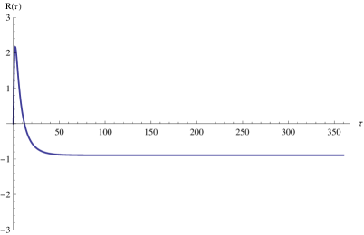
  (a) $\theta_{1}=-0.3,\theta_{2}=0.9,X(t)=-0.5,Y(t)=0.5$

  

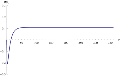
  (b) $\theta_{1}=0.03,\theta_{2}=-0.9,X(t)=0.5,Y(t)=0.5$

  

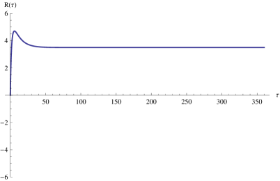
  (c) $\theta_{1}=-0.09,\theta_{2}=0.9,X(t)=-0.5,Y(t)=0.5$

  

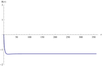
  (d) $\theta_{1}=-0.2,\theta_{2}=0.1,X(t)=0.5,Y(t)=0.5$

  Figure 5. Risk premium profiles when $L$ is a compound Poisson process with exponentially distributed jumps. Esscher transform: case $\bar{\beta}=(0,0).$ Geometric spot model

  If $\theta_{2}=0,$ then the sign of $R_{g,Q}^{F}(t,\tau)$ is the same as the sign of $\theta_{1}$ and it is constant over all times to maturity $\tau.$ Similarly, if $\theta_{1}=0,$ the sign $R_{g,Q}^{F}(t,\tau)$ is the same as the sign of $\theta_{2}$ and it is also constant. If both $\theta_{1}$ and $\theta_{2}$ are different from zero we can get risk premium profiles with non constant sign. By Lemma 4.19, we have that

  $$\lim_{\tau\rightarrow 0}\frac{\partial}{\partial\tau}\Sigma(t,\tau) =\theta_{1}+\kappa_{L}(1+\theta_{2})-\kappa_{L}(\theta_{2})-\kappa_{L}(1)$$

  $$=\theta_{1}+\int_{0}^{\infty}(e^{\theta_{2}z}-1)(e^{z}-1)\ell(dz).$$

  Hence, if we want the sign of $R_{g,Q}^{F}(t,\tau)$ to be positive when $\tau$ is close to zero we have to impose

  $$\theta_{1}+\int_{0}^{\infty}(e^{\theta_{2}z}-1)(e^{z}-1)\ell(dz)>0.$$ (4.32)

  For large times to maturity, Lemma 4.19 yields

  $$\lim_{\tau\rightarrow\infty}\Sigma(t,\tau) =\frac{\theta_{1}}{\alpha_{X}}+\int_{0}^{\infty}\kappa_{L}(e^{-\alpha_{Y}t}+\theta_{2})-\kappa_{L}(\theta_{2})-\kappa_{L}(e^{-\alpha_{Y}t})dt$$

  $$=\frac{\theta_{1}}{\alpha_{X}}+\int_{0}^{\infty}\int_{0}^{\infty}(e^{\theta_{2}z}-1)(e^{ze^{-\alpha_{Y}t}}-1)\ell(dz)dt.$$

  Using Fubini’s theorem we get that

  $$\int_{0}^{\infty}\int_{0}^{\infty}(e^{\theta_{2}z}-1)(e^{ze^{-\alpha_{Y}t}}-1)\ell(dz)dt$$

  $$=\int_{0}^{\infty}(e^{\theta_{2}z}-1)\int_{0}^{\infty}(e^{ze^{-\alpha_{Y}t}}-1)dt\ell(dz)$$

  $$=\int_{0}^{\infty}\frac{(e^{\theta_{2}z}-1)}{\alpha_{Y}}\left(\operatorname{Ei}(z)-\log(z)-\gamma\right)\ell(dz),$$

  where $\operatorname{Ei}(z)=\int_{-\infty}^{z}\frac{e^{t}}{t}dt$ is the exponential integral function and $\gamma$ is the Euler-Mascheroni constant. Hence, if we want $R_{g,Q}^{F}(t,\tau)$ to be negative when $\tau$ is large we have to impose

  $$\theta_{1}+\frac{\alpha_{X}}{\alpha_{Y}}\int_{0}^{\infty}(e^{\theta_{2}z}-1)\left(\operatorname{Ei}(z)-\log(z)-\gamma\right)\ell(dz)<0.$$ (4.33)

  Note that $\operatorname{Ei}(z)-\log(z)-\gamma\geq 0,\forall z\geq 0$ and $e^{z}-1-\frac{\alpha_{X}}{\alpha_{Y}}\left(\operatorname{Ei}(z)-\log(z)-\gamma\right)>0,$ for all $z>0$ and $\alpha_{X}<\alpha_{Y}.$Therefore, for all $\theta_{2}>0$ one has that

  $$0<\int_{0}^{\infty}(e^{\theta_{2}z}-1)\left(\operatorname{Ei}(z)-\log(z)-\gamma\right)\ell(dz)<\frac{\alpha_{Y}}{\alpha_{X}}\int_{0}^{\infty}(e^{\theta_{2}z}-1)\left(e^{z}-1\right)\ell(dz).$$ (4.34)

  Combining equations $\left(\ref{Equ_GeomSmallTau}\right)$, $\left(\ref{Equ_GeomLargeTau}\right)$ and $\left(\ref{Equ_inequality_IntegralsEi}\right)$ we can conclude that it is possible to choose $\theta_{1}<0$ and $\theta_{2}>0$ such that $R_{g,Q}^{F}(t,\tau)>0$ when the time to maturity is close to zero and $R_{g,Q}^{F}(t,\tau)<0$ when the time to maturity is large.

• Changing the speed of mean reversion, $\bar{\theta}=(0,0):$ Setting $\bar{\theta}=(0,0),$ the probability measure $Q$ only changes the speed of mean reversion. By Lemma 4.19 we have that the sign of $R_{g,Q}^{F}(t,\tau)$ will coincide with the sign of

  $$\Sigma(t,\tau) =X(t)e^{-\alpha_{X}\tau}(e^{\alpha_{X}\beta_{1}\tau}-1)+Y(t)\left(\Psi_{0,\beta_{2}}^{1}(\tau)-\Psi_{0,0}^{1}(\tau)\right)$$

  $$+\frac{\sigma_{X}^{2}}{4\alpha_{X}}\Lambda(2\alpha_{X}\tau,1-\beta_{2})+\left(\Psi_{0,\beta_{2}}^{0}(\tau)-\Psi_{0,0}^{0}(\tau)\right)$$

  $$\triangleq\Sigma_{1}(t,\tau)+\Sigma_{2}(t,\tau)+\Sigma_{3}(t,\tau)+\Sigma_{4}(t,\tau),$$

  and

  

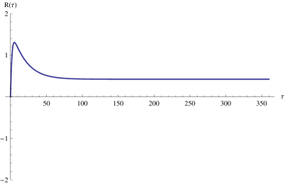
  (a) $\beta_{1}=0.4,\beta_{2}=0.2,X(t)=1.0,Y(t)=0.5$

  

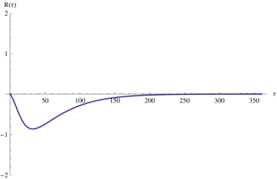
  (b) $\beta_{1}=0.75,\beta_{2}=0.0,X(t)=-2.5,Y(t)=0.5$

  

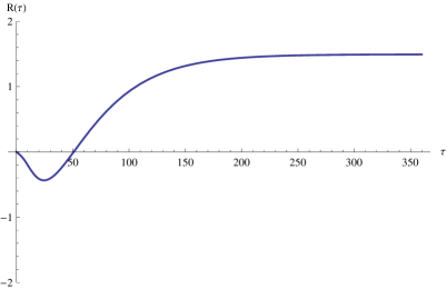
  (c) $\beta_{1}=0.75,\beta_{2}=0.3,X(t)=-2.5,Y(t)=0.0$

  

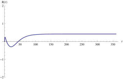
  (d) $\beta_{1}=0.5,\beta_{2}=0.2,X(t)=-2.5,Y(t)=2.5$

  Figure 6. Risk premium profiles when $L$ is a compound Poisson process with exponentially distributed jumps. Case $\bar{\theta}=(0,0).$ Geometric spot price model

  $$\lim_{\tau\rightarrow\infty}\Sigma(t,\tau) =\frac{\sigma_{X}^{2}}{4\alpha_{X}}\frac{\beta_{1}}{1-\beta_{1}}\geq 0$$

  $$\lim_{\tau\rightarrow 0}\frac{\partial}{\partial\tau}\Sigma(t,\tau) =X(t)\alpha_{X}\beta_{1}+Y(t)\alpha_{Y}\beta_{2}\frac{\kappa_{L}^{\prime}(1)-\kappa_{L}^{\prime}(0)}{\kappa_{L}^{\prime\prime}(0)},$$

  where $\kappa_{L}^{\prime}(1)-\kappa_{L}^{\prime}(0)$ and $\kappa_{L}^{\prime\prime}(0)$ are strictly positive. Hence the risk premium will approach to a non negative value in the long end of the market. In the short end, it can be both positive or negative and stochastically varying with $X(t)$ and $Y(t),$ but $Y(t)$ will always contribute to a positive sign. For any $\tau,$ the sign of $\Sigma_{1}(t,\tau)$ will be the sign of $X(t),$ that can be positive or negative. As the function $\Lambda(x,y)\$is positive, the term $\Sigma_{3}(t,\tau)$ is always positive. To analyse the sign of $\Sigma_{2}(t,\tau),$ note that

  $$\Lambda_{1}^{0,\beta_{2}}(u)-\Lambda_{1}^{0,0}(u)=\frac{\alpha_{Y}\beta_{2}}{\kappa_{L}^{\prime\prime}(0)}\int_{0}^{\infty}(e^{uz}-1)z\ell(dz)\geq 0,\quad u\geq 0,$$

  and $\Psi_{0,\beta_{2}}^{1}(1)=\Psi_{0,0}^{1}(\tau).$ Hence, applying a comparison theorem for ODEs, see Theorem 6.1, pag.31, in Hale [12], we have that $\Psi_{0,\beta_{2}}^{1}(\tau)-\Psi_{0,0}^{1}(\tau)\geq 0,$ for all $\tau,$ and, as $Y(t)$ is always positive, the term $\Sigma_{2}(t,\tau)$ is also always positive. Finally, as

  $$\Lambda_{0}(u)\triangleq\Lambda_{0}^{0,\beta_{2}}(u)=\Lambda_{0}^{0,0}(u)=\int_{0}^{\infty}(e^{uz}-1)\ell(dz),$$

  is an strictly increasing function and $\Psi_{0,\beta_{2}}^{1}(t)\geq\Psi_{0,0}^{1}(t)$ we get that

  $$\Sigma_{4}(t,\tau)=\Psi_{0,\beta_{2}}^{0}(\tau)-\Psi_{0,0}^{0}(\tau)=\int_{0}^{\tau}\{\Lambda_{0}(\Psi_{0,\beta_{2}}^{1}(t))-\Lambda_{0}(\Psi_{0,0}^{1}(t))\}dt\geq 0.$$

  Hence, if $\beta_{1}=0$ or $X(t)\geq 0,$ then $R_{g,Q}^{F}(t,\tau)$ will be positive for all times to maturity. Some of the possible risk profiles that can be obtained are plotted in Figure 6.

• Changing the level and speed of mean reversion simultaneously: We proceed as in the arithmetic case. As we are more interested in how the change of measure $Q$ influence the component $Y(t)$, responsible for the spikes in the prices, we are going to assume that $\beta_{1}=0.$ This means that $Q$ may change the level of mean reversion of the regular component $X(t),$ but not the speed at which this component reverts to that level. According to Lemma 4.19 we have that the sign of $R_{g,Q}^{F}(t,\tau)$ will coincide with the sign of

  $$\Sigma(t,\tau) =Y(t)(\Psi_{\theta_{2},\beta_{2}}^{1}(\tau)-e^{-\alpha_{Y}\tau})+\frac{\theta_{1}}{\alpha_{X}}(1-e^{-\alpha_{X}\tau})+\Psi_{\theta_{2},\beta_{2}}^{0}(\tau)$$

  $$-\int_{0}^{\tau}\int_{0}^{\infty}(e^{ze^{-\alpha_{Y}s}}-1)\ell(dz)ds$$

  $$=Y(t)\left(\Psi_{\theta_{2},\beta_{2}}^{1}(\tau)-\Psi_{0,0}^{1}(\tau)\right)+\frac{\theta_{1}}{\alpha_{X}}(1-e^{-\alpha_{X}\tau})+\left(\Psi_{\theta_{2},\beta_{2}}^{0}(\tau)-\Psi_{0,0}^{0}(\tau)\right)$$

  $$\triangleq\Sigma_{1}(t,\tau)+\Sigma_{2}(t,\tau)+\Sigma_{3}(t,\tau),$$

  and

  $$\lim_{\tau\rightarrow\infty}\Sigma(t,\tau) =\frac{\theta_{1}}{\alpha_{X}}+\int_{0}^{\infty}\kappa_{L}(\Psi_{\theta_{2},\beta_{2}}^{1}(t)+\theta_{2})-\kappa_{L}(\theta_{2})-\kappa_{L}(e^{-\alpha_{Y}t})dt$$ (4.35)

  $$=\frac{\theta_{1}}{\alpha_{X}}+\int_{0}^{\infty}\int_{0}^{1}\kappa_{L}^{\prime}(\theta_{2}+\lambda\Psi_{\theta_{2},\beta_{2}}^{1}(t))d\lambda\Psi_{\theta_{2},\beta_{2}}^{1}(t)dt$$

  $$-\int_{0}^{\infty}\int_{0}^{1}\kappa_{L}^{\prime}(\theta_{2}+\lambda e^{-\alpha_{Y}t})d\lambda e^{-\alpha_{Y}t}dt$$

  $$\lim_{\tau\rightarrow 0}\frac{\partial}{\partial\tau}\Sigma(t,\tau) =Y(t)\alpha_{Y}\beta_{2}\frac{\kappa_{L}^{\prime}(1+\theta_{2})-\kappa_{L}^{\prime}(\theta_{2})}{\kappa_{L}^{\prime\prime}(\theta_{2})}$$ (4.36)

  $$+\theta_{1}+\kappa_{L}(1+\theta_{2})-\kappa_{L}(\theta_{2})-\kappa_{L}(1)$$

  $$=Y(t)\alpha_{Y}\beta_{2}\frac{\kappa_{L}^{\prime}(1+\theta_{2})-\kappa_{L}^{\prime}(\theta_{2})}{\kappa_{L}^{\prime\prime}(\theta_{2})}+\theta_{1}$$

  $$+\int_{0}^{1}\kappa_{L}^{\prime}(\theta_{2}+\lambda)d\lambda-\kappa_{L}(1)$$

  

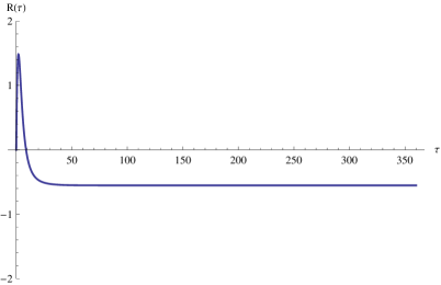
  (a) $\beta_{1}=0,\beta_{2}=0.2,\theta_{1}=-0.1,\theta_{2}=0.2,X(t)=1.0,Y(t)=1.0$

  Figure 7. Risk premium profiles when $L$ is a compound Poisson process with exponentially distributed jumps. Geometric spot model

  Note that we can make equation $\left(\ref{Equ_RPG_General_1}\right)$ negative by simply choosing $\theta_{1}$

  $$\theta_{1} <-\alpha_{X}\int_{0}^{\infty}\int_{0}^{1}\kappa_{L}^{\prime}(\theta_{2}+\lambda\Psi_{\theta_{2},\beta_{2}}^{1}(t))d\lambda\Psi_{\theta_{2},\beta_{2}}^{1}(t)dt$$ (4.37)

  $$+\alpha_{X}\int_{0}^{\infty}\int_{0}^{1}\kappa_{L}^{\prime}(\theta_{2}+\lambda e^{-\alpha_{Y}t})d\lambda e^{-\alpha_{Y}t}dt.$$

  On the other hand, to make equation $(\ref{Equ_RPG_General_2})$ positive, we have to choose $\theta_{1}$ satisfying

  $$\theta_{1}>-\int_{0}^{1}\kappa_{L}^{\prime}(\theta_{2}+\lambda)d\lambda+\kappa_{L}(1)-Y(t)\alpha_{Y}\beta_{2}\frac{\kappa_{L}^{\prime}(1+\theta_{2})-\kappa_{L}^{\prime}(\theta_{2})}{\kappa_{L}^{\prime\prime}(\theta_{2})}.$$ (4.38)

  Equations $\left(\ref{Equ_RPG_General_3}\right)$ and $\left(\ref{Equ_RPG_General_4}\right)$ are compatible if the following equation is satisfied

  $$U_{+}(\theta_{2},\beta_{2}) \triangleq\int_{0}^{1}\kappa_{L}^{\prime}(\theta_{2}+\lambda)d\lambda+\alpha_{X}\int_{0}^{\infty}\int_{0}^{1}\kappa_{L}^{\prime}(\theta_{2}+\lambda e^{-\alpha_{Y}t})d\lambda e^{-\alpha_{Y}t}dt$$

  $$+Y(t)\alpha_{Y}\beta_{2}\frac{\kappa_{L}^{\prime}(1+\theta_{2})-\kappa_{L}^{\prime}(\theta_{2})}{\kappa_{L}^{\prime\prime}(\theta_{2})}$$

  $$>\alpha_{X}\int_{0}^{\infty}\int_{0}^{1}\kappa_{L}^{\prime}(\theta_{2}+\lambda\Psi_{\theta_{2},\beta_{2}}^{1}(t))d\lambda\Psi_{\theta_{2},\beta_{2}}^{1}(t)dt+\kappa_{L}(1)\triangleq U_{-}(\theta_{2},\beta_{2}).$$ (4.39)

  As $e^{-\alpha_{Y}t}\leq 1,\Psi_{\theta_{2},\beta_{2}}^{1}(t)\leq 1,\kappa_{L}^{\prime}(\theta)>0$ and $\kappa_{L}^{\prime\prime}(\theta)>0$ we have that

  $$\frac{\kappa_{L}^{\prime}(1+\theta_{2})-\kappa_{L}^{\prime}(\theta_{2})}{\kappa_{L}^{\prime\prime}(\theta_{2})} =\frac{\int_{0}^{1}\kappa_{L}^{\prime\prime}(\theta_{2}+\lambda)d\lambda}{\kappa_{L}^{\prime\prime}(\theta_{2})}>1,$$

  $$\int_{0}^{\infty}\int_{0}^{1}\kappa_{L}^{\prime}(\theta_{2}+\lambda e^{-\alpha_{Y}t})d\lambda e^{-\alpha_{Y}t}dt \geq\frac{\kappa_{L}^{\prime}(\theta_{2})}{\alpha_{Y}},$$

  and

  $$\int_{0}^{\infty}\int_{0}^{1}\kappa_{L}^{\prime}(\theta_{2}+\lambda\Psi_{\theta_{2},\beta_{2}}^{1}(t))d\lambda\Psi_{\theta_{2},\beta_{2}}^{1}(t)dt\leq\int_{0}^{1}\kappa_{L}^{\prime}(\theta_{2}+\lambda)d\lambda\int_{0}^{\infty}\Psi_{\theta_{2},\beta_{2}}^{1}(t)dt,$$

  As $\Psi_{\theta_{2},\beta_{2}}^{1}(t)$ converges to zero exponentially fast, see equation $\left(\ref{Equ_Exp_Psi1}\right)$, we have that

  $$\int_{0}^{\infty}\Psi_{\theta_{2},\beta_{2}}^{1}(t)dt<\infty.$$

  Actually, as $\Lambda_{1}^{\theta_{2},\beta_{2}}(u)<\Lambda_{1}^{\theta_{2},\beta_{2}}(1)<0,0<u<1,$ we can use a comparison theorem for ODEs to obtain that

  $$\Psi_{\theta_{2},\beta_{2}}^{1}(t)\leq e^{\Lambda_{1}^{\theta_{2},\beta_{2}}(1)t}=\exp\left(-\alpha_{Y}(1-\frac{\beta_{2}}{\kappa_{L}^{\prime\prime}(\theta_{2})}(\kappa_{L}^{\prime}(1+\theta_{2})-\kappa_{L}^{\prime}(\theta_{2})))t\right),$$

  which yields

  $$\int_{0}^{\infty}\Psi_{\theta_{2},\beta_{2}}^{1}(t)dt\leq\frac{1}{\alpha_{Y}}(1-\beta_{2}\frac{\int_{0}^{1}\kappa_{L}^{\prime\prime}(\theta_{2}+\lambda)d\lambda}{\kappa_{L}^{\prime\prime}(\theta_{2})})^{-1}.$$

  Hence,

  $$U_{+}(\theta_{2},\beta_{2}) \geq\int_{0}^{1}\kappa_{L}^{\prime}(\theta_{2}+\lambda)d\lambda+\frac{\alpha_{X}}{\alpha_{Y}}\kappa_{L}^{\prime}(\theta_{2})+Y(t)\alpha_{Y}\beta_{2}\triangleq V_{+}(\theta_{2},\beta_{2}),$$

  $$U_{-}(\theta_{2},\beta_{2}) \leq\frac{\alpha_{X}}{\alpha_{Y}}\int_{0}^{1}\kappa_{L}^{\prime}(\theta_{2}+\lambda)d\lambda(1-\beta_{2}\frac{\int_{0}^{1}\kappa_{L}^{\prime\prime}(\theta_{2}+\lambda)d\lambda}{\kappa_{L}^{\prime\prime}(\theta_{2})})^{-1}+\kappa_{L}(1)\triangleq V_{-}(\theta_{2},\beta_{2}),$$

  and if we can find $\theta_{2}\in D_{L}^{g}(\delta)$ for some $\delta>0$ and $\beta_{2}\in(0,1)$ such that $V_{+}(\theta_{2},\beta_{2})>V_{-}(\theta_{2},\beta_{2})$ then equation $\left(\ref{Equ_RPG_General_5}\right)$ will be satisfied. Note that the larger the value of $Y(t)$ the easier to find such $\theta_{2}$ and $\beta_{2}.$ Even in the case that $Y(t)=0,$ by choosing $\beta_{2}$ close to zero and $\theta_{2}$ large enough we can get $V_{+}(\theta_{2},\beta_{2})>V_{-}(\theta_{2},\beta_{2}).$ This shows that we can create a change of measure $Q$ generating the empirically observed risk premium profile, see Figure 7.

References

- [1] Barndorff-Nielsen, O.E., Benth, F.E., and Veraart, A. (2010). Modelling energy spot prices by volatility modulated Levy-driven Volterra processes. Bernoulli 19 (3), pp. 803–845.
- [2] Benth, F.E., Šaltytė Benth, J. and Koekebakker, S. (2008). Stochastic Modelling of Electricity and Related Markets. World Scientific.
- [3] Benth, F.E., Cartea, A., and Kiesel, R. (2008). Pricing forward contracts in power markets by the certainty equivalence principle: explaining the sign of the market risk premium. Journal of Banking and Finance, 32(10), pp. 2006–2021.
- [4] Benth, F.E. and Sgarra, C. (2012). The Risk Premium and the Esscher Transform in Power Markets. Stochastic Analysis and Applications 30, pp. 20–43.
- [5] Bessembinder, H., and Lemon, M.L. (2002). Equilibrium pricing and optimal hedging in electricity forward markets. Journal of Finance, 57, pp. 1347–1382.
- [6] Bingham, N., and Kiesel, R. (1998). Risk-Neutral Valuation. Pricing and Hedging of Financial Derivatives. Springer-Verlag.
- [7] Cartea, A., and Figueroa, M.G. (2005). Pricing in electricity markets: a mean reverting jump diffusion model with seasonality. Applied Mathematical Finance, 12(3), pp. 313–335.
- [8] Cont, R. and Tankov, P. (2004). Financial Modelling with Jump Processes. Chapman & Hall/CRC
- [9] Geman, H. (2005). Commodities and Commodity Derivatives. Wiley-Finance.
- [10] Geman, H., and Vasicek, O. (2001). Forwards and futures on non storable commodities: the case of electricity. RISK, August.
- [11] Gibson, R., and Schwartz, E.S. (1990). Stochastic convenience yield and the pricing of oil contingent claims. Journal of Finance, 45, pp. 959–976.
- [12] Hale, J. (1969). Ordinary Differential Equations, Pure and Applied Mathematics, Vol. XXI. Wiley-Interscience.
- [13] Ikeda, N. and Watanabe, S. (1981). Stochastic Differential Equations and Diffusion Processes, North-Holland.
- [14] Jacod, J. and Shiryaev, A.N. (2003). Limit Theorems for Stochastic Processes, Springer.
- [15] Kallsen, J. and Muhle-Karbe J. (2010). Exponentially affine martingales, affine measure changes and exponential moments of affine processes. Stochastic Processes and their Applications 120, pp. 163–181.
- [16] Kallsen, J. and Shiryaev, A. (2002). The cumulant process and Esscher’s change of measure. Finance & Stochastics 6, pp. 397–428.
- [17] Kazamaki, N. (1977). On a problem of Girsanov. Tôhoku Math. J. 29 (4), pp. 597–600.
- [18] Klebaner, F. and Lipster, R. (2011). When a stochastic exponential is a true martingale. Extension of a method of Beneŝ. arXiv:1112.0430v1.
- [19] Lepingle, D. and Mémin, J. (1978). Sur l’intégrabilité uniforme des martingales exponentielles, Z. Wahrscheinlichkeitstheorie verw. Gebiete 42, pp. 175–203.
- [20] Lucia, J., and Schwartz, E.S. (2002). Electricity prices and power derivatives: evidence from the Nordic power exchange. Review of Derivatives Research, 5(1), pp. 5–50.
- [21] Novikov, A. (1980). On conditions for uniform integrability of continuous non-negative martingales. Theory of Probability and its Applications 24, pp. 820–824.
- [22] Sato, K. (1999). Lévy Processes and Infinitely Divisible Distributions. Cambridge Studies in Advanced Mathematics.
- [23] Schwartz, E.S., and Smith, J.E. (2000). Short-term variations and long-term dynamics in commodity prices. Management Science, 46(7), pp. 893–911.
- [24] Shiryaev, A. N. (1999). Essentials of Stochastic Finance, World Scientific.