Using Coordinated Observations in Polarised White Light and Faraday Rotation to Probe the Spatial Position and Magnetic Field of an Interplanetary Sheath

Abstract

Coronal mass ejections (CMEs) can be continuously tracked through a large portion of the inner heliosphere by direct imaging in visible and radio wavebands. White-light (WL) signatures of solar wind transients, such as CMEs, result from Thomson scattering of sunlight by free electrons, and therefore depend on both the viewing geometry and the electron density. The Faraday rotation (FR) of radio waves from extragalactic pulsars and quasars, which arises due to the presence of such solar wind features, depends on the line-of-sight magnetic field component $B_{\parallel}$, and the electron density. To understand coordinated WL and FR observations of CMEs, we perform forward magnetohydrodynamic modelling of an Earth-directed shock and synthesise the signatures that would be remotely sensed at a number of widely distributed vantage points in the inner heliosphere. Removal of the background solar wind contribution reveals the shock-associated enhancements in WL and FR. While the efficiency of Thomson scattering depends on scattering angle, WL radiance $I$ decreases with heliocentric distance $r$ roughly according to the expression $I\propto r^{-3}$. The sheath region downstream of the Earth-directed shock is well viewed from the L4 and L5 Lagrangian points, demonstrating the benefits of these points in terms of space weather forecasting. The spatial position of the main scattering site $\mathbf{r}_{\rm sheath}$ and the mass of plasma at that position $M_{\rm sheath}$ can be inferred from the polarisation of the shock-associated enhancement in WL radiance. From the FR measurements, the local $B_{\parallel{\rm sheath}}$ at $\mathbf{r}_{\rm sheath}$ can then be estimated. Simultaneous observations in polarised WL and FR can not only be used to detect CMEs, but also to diagnose their plasma and magnetic field properties.

1. Introduction

1.1. The Inner Heliosphere

The inner heliosphere is permeated with the magnetised solar wind from the Sun. At solar minimum, the solar wind is inherently bimodal (McComas et al. 2000), with slow flow tending to emanate from near the ecliptic and fast flow tending to emanate at higher latitudes. Several large-scale structures, which pervade interplanetary space, are associated with the “ambient” solar wind: (1) a spiralling interplanetary magnetic field (the Parker spiral) that forms as a result of solar rotation (Parker 1958), (2) corotating interacting regions (CIRs) that are formed at the interface between a preceding slow solar wind stream and a following fast solar wind stream (Gosling & Pizzo 1999), and (3) the heliospheric current sheet typically embedded in the heliospheric plasma sheet (Winterhalter et al. 1994; Crooker et al. 2004).

The background solar wind flow is frequently disturbed by coronal mass ejections (CMEs), large-scale expulsions of plasma and magnetic field from the solar atmosphere. CMEs typically expand during their propagation, because the total solar wind pressure decreases with heliocentric distance (Démoulin & Dasso 2009; Gulisano et al. 2010). The expansion speed of a CME depends on its spatial size, translation speed, and heliocentric distance, as well as the pre-existing solar wind conditions (Nakwacki et al. 2011; Gulisano et al. 2012). A number of popular models describe the motion of a CME as governed by two forces: a propelling Lorentz force (Chen 1989, 1996; Chen et al. 2006) and an aerodynamic drag force (Cargill et al. 1996; Vršnak & Gopalswamy 2002; Cargill 2004). According to these models, the drag force gradually becomes dominant in interplanetary space, and the CME speed finally adjusts to the ambient solar wind speed. The equalisation of the CME and solar wind speed occurs at very different heliospheric distances, from below 30 solar radii to beyond 1 AU, depending on the characteristics of the CME and the solar wind (Temmer et al. 2011). A CME can undergo significant, nonlinear, and irreversible evolution during its propagation, as it interacts with the ambient solar wind and other CMEs (e.g., Burlaga et al. 2002; Démoulin 2010). Coronagraph observations show that CME morphology is distorted rapidly and significantly in a structured solar wind (e.g., Savani et al. 2010, 2012; Feng et al. 2012a). Such a distortion occurs over a relatively short heliocentric distance. Interaction between multiple CMEs has been revealed by in-situ observations (e.g., Burlaga et al. 1987; Wang et al. 2003a; Steed et al. 2011; Möstl et al. 2012), radio burst observations (e.g., Gopalswamy et al. 2001; Oliveros et al. 2012), white-light (WL) imaging (e.g., Harrison et al. 2012; Liu et al. 2012; Lugaz et al. 2012; Temmer et al. 2012; Shen et al. 2012a; Bemporad et al. 2012), and numerical magnetohydrodynamic (MHD) simulation (e.g., Lugaz et al. 2005; Xiong et al. 2007, 2009; Shen et al. 2012b).

CMEs cause phenomena at Earth, such as geomagnetic storms and solar energetic particles, that can result in major space weather effects (Gopalswamy 2006; Webb & Howard 2012). Traditionally, a CME has been defined in terms of a three-part structure, involving a bright sheath, a dark cavity, and a bright filament. It is now accepted that the cavity component is an escaping magnetic flux rope that drives the CME (e.g., Rouillard et al. 2009b; DeForest et al. 2011). A high-speed flux rope can drive a fast shock ahead of itself that is much wider in angular extent than the flux rope itself. The region between the shock front and the flux rope is defined as a sheath. Within the sheath, (1) magnetic field lines are draped and compressed, and (2) a plasma flow is deviated, compressed, and turbulent (e.g., Gosling & McComas 1987; Owens et al. 2005; Liu et al. 2008). Precursor southward magnetic fields ahead of CMEs are generally compressed, making them particularly geoeffective (Tsurutani et al. 1992; Gonzalez et al. 1999). The magnetic fields in the sheath and in the flux rope can be equally important in driving major geomagnetic storms (Tsurutani et al. 1988, 1992; Szajko et al. 2013). In so-called two-dip storms, it is often the case that the first dip in the $Dst$ index is produced by the upstream sheath and the second is produced by the driving flux rope (Echer et al. 2004; Zhang et al. 2008; Möstl et al. 2012).

1.2. Heliospheric White Light Observations

Heliospheric imagers (HIs) detect WL that has been Thomson-scattered from free electrons. For resolved objects, such as CMEs, the power detected by an individual pixel depends linearly on the solid angle subtended by that pixel ($\delta\omega$) and the area subtended by the corresponding aperture ($\delta A$), and is proportional to the radiance (measured in W m^-2 SR^-1). The light from unresolved objects, such as stars, which are much narrower in angular extent, tends to fall within individual pixels. For a resolved heliospheric electron density feature, such as a CME, a single pixel provides a measure of its radiance (surface brightness), while summing contributions from all pixels over the entire extent of the feature provides a measure of its intensity (total brightness). The intensity is an integral of the radiance over the apparent feature size. Therefore, the feature’s intensity determines its detectability of an object, be it resolved or unresolved (Howard & DeForest 2012).

The background zodiacal and stellar signals detected by heliospheric imagers are much more intense than the signal due to Thomson-scattering from plasma features such as CMEs (Leinert & Pitz 1989). Fortunately, using an image-differencing technique, the much more stable background radiance can be removed, such that the more transient Thomson-scattering signal can be extracted. From such processed Thomson-scattering images, the sunlight-irradiated CMEs can be easily identified and tracked. According to theory, the heliospheric Thomson-scattering radiance is governed by the Thomson-scattering geometry factors and electron number density (Vourlidas & Howard 2006; Howard & Tappin 2009; Howard & DeForest 2012; Xiong et al. 2013). The CME detectability in WL is actually more limited by perspective and field-of-view (FOV) effects than by location relative to the Thomson-scattering sphere (Howard & DeForest 2012).

Heliospheric imaging from two vantage points, both off the Sun-Earth line, was made possible by the Heliospheric Imagers (HIs) onboard the Solar-TErrestrial RElations Observatory (STEREO) (Eyles et al. 2009). With the STEREO/SECCHI package, a CME can be imaged from its nascent stage in the inner corona all the way out to 1 AU and beyond (e.g., Harrison et al. 2008; Davies et al. 2009; Davis et al. 2009; Liu et al. 2010b; DeForest et al. 2011; Liu et al. 2013). In particular, images from STEREO/HI-2 have revealed detailed spatial structures within interplanetary CMEs, including leading-edge pileup, interior cavities, filamentary structure, and rear cusps (DeForest et al. 2011). Comparison with in-situ observations has revealed that the leading-edge pileup of solar wind material, which is evident as a bright arc in WL imaging, corresponds to the sheath region. However, the interpretation of the leading edge of the radiance pattern, especially at larger elongations, is fraught with ambiguity (e.g., Howard & Tappin 2009; Xiong et al. 2013). Elongation $\varepsilon$ is defined as the angle between the Sun-observer line and a line-of-sight (LOS). Because a CME occupies a significant three-dimensional (3D) volume, different parts of the CME will contribute to the radiance pattern imaged by observers situated at different heliocentric longitudes (Xiong et al. 2013). Even for an observer at a fixed longitude, a different part of the CME will contribute to the imaged radiance at any given time (Xiong et al. 2013). Various techniques have been developed that enable the spatial locations and propagation directions of CMEs to be inferred, based on the fitting of their moving radiance patterns (e.g., Sheeley et al. 2008; Rouillard et al. 2008; Thernisien et al. 2009; Liu et al. 2010b; Lugaz et al. 2010; Möstl et al. 2011; Davies et al. 2012). However, the determination of interplanetary CME kinematics, propagation direction in particular, are somewhat ambiguous (Howard & Tappin 2009; Davis et al. 2010; Davies et al. 2012; Howard & DeForest 2012; Xiong et al. 2013; Lugaz & Kintner 2013).

1.3. Faraday Rotation Measurement

Faraday rotation (FR) is the rotation of the plane of polarisation of an incident electromagnetic wave as it passes through a magnetised ionic medium. The FR observations of linearly polarised radio sources can be used to estimate magnetic field in the corona and interplanetary space (e.g., Levy et al. 1969; Bird et al. 1980; Sakurai & Spangler 1994; Liu et al. 2007; Jensen 2007; Jensen & Russell 2008; You et al. 2012; Jensen et al. 2013). The FR measurement of a radio signal corresponds to the path integral of the product of electron density $n$ and the projection of the magnetic field along the LOS, $B_{\parallel}$. The first FR experiment was conducted in 1968 by Levy et al. (1969), when solar plasma occulted the radio down-link from the Pioneer 6 spacecraft. As well as man-made radio sources, FR experiments can also exploit natural radio sources such as pulsars and quasars. The first FR experiments of this type were conducted by Bird et al. (1980) during the solar occultation of a pulsar. In terms of their locations on a sky map, many pulsars and quasars lie in the vicinity of the Sun. Therefore, simultaneous FR measurements along multiple beams can be used to map the inner heliosphere with a reasonable spatial resolution.

Additional observations, for example in WL, would generally be necessary to confirm whether an FR transient was indeed caused by a CME. For instance, the first FR event, reported by Levy et al. (1969), could not be attributed unambiguously to the presence of any particular solar wind structure. The FR signatures, observed by Levy et al. (1969), exhibited a W-shaped profile over a time period of $2-3$ hours, with rotation angles of up to 40^∘ relative to the quiescent baseline. Woo (1997) interpreted the FR signature as the result of a coronal streamer stalk of angular size $1^{\circ}-2^{\circ}$, whereas Pätzold & Bird (1998) argued that it was caused by the passage of a series of CMEs. However, by comparing observations from the Solwind coronagraph and measurements of Helios down-link radio signals, Bird et al. (1985) were able to identify the signatures of five CMEs simultaneously in WL and FR. Moreover, the electron density derived from WL imaging can be used to enable magnetic field magnitude to be inferred from FR measurements.

The heliospheric magnetic field can be remotely probed in FR, using low-frequency radio interferometers such as the Murchison Widefield Array (MWA) (Lonsdale, C. J., et. al. 2009), the LOw Frequency ARray (LOFAR) (de Vos et al. 2009), and the Very Large Array (VLA) (Thompson et al. 1980). Disturbance of the background solar wind by CMEs will cause the observed FR signatures to become variable (e.g., Levy et al. 1969; Bird et al. 1985; Jensen & Russell 2008). A change in either the electron density ($\delta n$) or the LOS magnetic field component ($\delta B_{\parallel}$), or indeed both, will contribute to the rotation in the plane of polarisation of the radio signal by $\delta\,\Omega_{\rm RM}$. Interplanetary magnetic clouds (MCs) in particular, which have a magnetic flux rope configuration (Burlaga et al. 1981; Klein & Burlaga 1982; Lepping et al. 1990), can be identified from WL images (Rouillard et al. 2009b; DeForest et al. 2011) and are expected to be easily identifiable in FR measurements. Moreover, $\delta n$ and $|\delta\mathbf{B}|$ are often enhanced simultaneously within the sheath ahead of a fast MC. The FR due to a MC-driven sheath can be comparable to that due to the MC itself (Jensen et al. 2010). It is expected that the orientation and helicity of a MC will be able to be determined unambiguously from multi-beam FR measurements (Liu et al. 2007; Jensen 2007; Jensen et al. 2010). In contrast, the in-situ detection of magnetic flux ropes can be significantly hindered by the location of the observing spacecraft (e.g., Hu & Sonnerup 2002; Möstl et al. 2012; Démoulin et al. 2013). FR imaging can be used to provide the magnetic orientation of a fast MC, and indeed its preceding sheath, prior to its arrival at Earth, which is crucial for predicting potential space weather effects at Earth.

1.4. Forward Magnetohydrodynamic Modelling

Forward modelling of WL and FR signatures is proving extremely useful for inferring the in-situ properties of interplanetary CMEs from remote-sensing data. Sophisticated numerical MHD models of the inner heliosphere (e.g., Groth et al. 2000; Lugaz et al. 2005; Hayashi 2005; Xiong et al. 2006a; Li et al. 2006; Wu et al. 2006; Li & Li 2008; Odstrčil & Pizzo 2009; Shen et al. 2012b) can serve as a digital laboratory, to enable the synthesis of a variety of observable remote-sensing signatures. In this paper, we perform a numerical MHD simulation of an interplanetary shock in the ecliptic, from which we synthesise the signatures of that feature that would be remotely sensed at visible and radio wavelengths. Details of the MHD model, and the formulae required to synthesise the remote-sensing observations, are given in Section 2. The resultant synthesised remote-sensing signatures of the sheath, which would be observed from vantage points at 0.5 and 1 AU, are described and compared in Section 3. In Section 4, we discuss the radiance patterns that are observed in the synthesised WL and FR sky maps. In Section 5, we explore the role that the vantage point of the observer plays in the “observability” of such WL and FR features. CME detection in the presence of background noise, and the heliospheric imaging of more complex interplanetary phenomena, are discussed in Section 6. The potentially important role that forward modelling can play in our understanding of coordinated WL and FR observations is summarised in Section 7.

2. Method

Forward MHD modelling can self-consistently establish the links between interplanetary dynamics and the resultant observable signatures. A complete flow chart of forward modelling is illustrated in Figure 8 from Xiong et al. (2011). The travelling fast shock studied by Xiong et al. (2013) is revisited here. Our methodology consists of three general steps: (1) forward modelling of the shock using the numerical Inner-Heliosphere MHD (IH-MHD) model (Xiong et al. 2006a, 2013), (2) calculation of its Thomson-scattered WL signature, in Section 2.1, and (3) calculation of its FR signature, in Section 2.2. Characterisation of the IH-MHD model, the background solar wind conditions, and the initial shock injection is summarised respectively in Tables 1, 2, and 3 of Xiong et al. (2013). The simulated electron density $n$ and magnetic field $\mathbf{B}$ are used to generate synthetic WL and FR images, which enable us to explore the WL and FR signatures of an interplanetary sheath.

A plasma parcel emitted from the Sun would be observed, at the same elongation and the same Thomson-scattering angle, firstly by an observer situated at a radial distance of 0.5 AU from the Sun centre, and subsequently by an observer at 1 AU (Figure 1a). Such a configuration was discussed qualitatively by Jackson et al. (2010) and is analysed quantitatively in Section 3 of this paper. Observations from STEREO/HI suggest that a travelling sheath can be approximated as an expanding bubble (e.g., Howard & Tappin 2009; Lugaz et al. 2010; Davies et al. 2012; Möstl & Davies 2013). In-situ observations indicate that CMEs undergo self-similar expansion, as the speed profiles within CMEs themselves tend to be a linear function of time (e.g., Farrugia et al. 1993; Gulisano et al. 2012). In the schematic Figures 1b-d, the sheath region following an Earth-directed interplanetary shock is represented as a self-similarly expanding bubble. The sheath can look quite different when viewed from different heliocentric distances (Figures 1b and 1c) and/or different heliospheric longitudes (Figures 1b and 1d).

2.1. Thomson-Scattering WL Formulae

A small parcel of free electrons, that is illuminated by a known intensity of incident sunlight (measured in W m^-2), will scatter a certain amount of power per unit solid angle (measured in W rad^-1). The effect of the Thomson-scattering geometry can be characterised by the so-called scattering angle $\chi$, as depicted in Figure 1 of Xiong et al. (2013). Scattering can be backward ($\chi<90^{\circ}$), perpendicular ($\chi=90^{\circ}$), and forward ($\chi>90^{\circ}$). All photons that are scattered into an optical cone defined by the point spread function of an individual pixel will be attributed to that pixel (Figure 1b, Xiong et al. 2013). The classic principles of WL Thomson-scattering, as applied to coronagraph observations (Billings 1966), have been adapted to heliospheric imaging (Vourlidas & Howard 2006; Howard & Tappin 2009; Jackson et al. 2010; Howard & DeForest 2012; Xiong et al. 2013). The transverse electric field oscillation $\delta\mathbf{E}$ of the Thomson-scattered radiance, which is inherently a continuum, can be considered in terms of its two orthogonal components, a tangential component $\delta\mathbf{E}_{\rm T}$ and a radial component $\delta\mathbf{E}_{\rm R}$. The amplitudes of these two orthogonal oscillations ($I_{\rm T}=|\delta\mathbf{E}_{\rm T}|^{2}$ and $I_{\rm R}=|\delta\mathbf{E}_{\rm R}|^{2}$) can be measured separately, using a polariser. The total radiance $I$ and degree of polarisation $p$ are defined as follows:

$$I=I_{\rm T}+I_{\rm R}$$ (1)

$$p=\frac{I_{\rm T}-I_{\rm R}}{I}$$ (2)

Although the incident sunlight is unpolarised ($p=0$), the scattered WL radiance remains unpolarised only when the scattering angle $|\chi-90^{\circ}|=90^{\circ}$. The scattered light is elliptically polarised ($0<p<1$) for $0^{\circ}<|\chi-90^{\circ}|<90^{\circ}$ and linearly polarised ($p=1$) for $\chi=90^{\circ}$. Each pixel of a detector records the LOS integral of local WL radiance.

$$\begin{array}[]{l}\left(\begin{array}[]{c}I\\ I_{\rm T}\\ I_{\rm R}\\ \end{array}\right)=\displaystyle\int^{\infty}_{0}\left(\begin{array}[]{c}i\\ i_{\rm T}\\ i_{\rm R}\\ \end{array}\right)dz=\displaystyle\int^{\infty}_{0}n\,z^{2}\left(\begin{array}[]{c}G\\ G_{\rm T}\\ G_{\rm R}\\ \end{array}\right)dz\end{array}$$ (3)

Here $z$ refers to a distance between the detector and the scattering site, as shown in Figure 1b of Xiong et al. (2013). The mathematical expressions for $G$, $G_{\rm R}$, and $G_{\rm T}$ are given by Equations 1 and 2 of Xiong et al. (2013). The observed WL radiance is determined jointly by the heliospheric distribution of electrons $n$ and Thomson-scattering geometry factors ($z^{2}G$, $z^{2}G_{\rm R}$, $z^{2}G_{\rm T}$).

As noted above, the efficiency of Thomson scattering depends significantly on the Thomson scattering angle $\chi$. The perpendicular scattering, $\chi=90^{\circ}$, received by an observer comes from the Thomson Sphere. The “Thomson sphere”, sometimes called the “Thomson surface”, is the sphere in which the Sun and observer lie at opposite ends of a diameter (e.g., Vourlidas & Howard 2006; Howard & DeForest 2012). The ecliptic cross sections of the Thomson scattering spheres for three observers are shown as dotted circles in Figures 1b-d. The LOS from an observer crosses its Thomson sphere at a so-called $p$ point (Figure 2, Tappin et al. 2004), where both the intensity of incident sunlight and local electron density are greatest, but the efficiency of Thomson scattering is least. Competition between these three effects results in the spread of local radiance ($i$, $i_{\rm T}$, $i_{\rm R}$ in Equation 3) to large distances from the Thomson surface, an effect that is greater at larger elongations $\varepsilon$ from the Sun. Howard & DeForest (2012) described this broad spreading effect, using the term “Thomson plateau”. Namely, along a single LOS, the radiance per unit electron density is virtually constant over a broad range of scattering angles $\chi$ centred at the $p$ point. The Thomson plateau, in terms of its relevance to heliospheric image, was discussed in detail by Howard & Tappin (2009), Howard & DeForest (2012), and Xiong et al. (2013).

A major milestone in stereoscopic WL imaging of interplanetary CMEs was achieved by the STEREO/HI instruments (e.g., Eyles et al. 2009; Davies et al. 2009; Davis et al. 2009; Harrison et al. 2009). This heliospheric imaging capability was built on the heritage of the Solar Mass Ejection Imager (SMEI) instrument on the Coriolis spacecraft (Eyles et al. 2003). The STEREO mission is comprised of two spacecraft, with one leading (STEREO A) and the other trailing (STEREO B) the Earth in its orbit. Both spacecraft separate from the Earth by $22.5^{\circ}$ per year. The HI instrument on each STEREO spacecraft consists of two cameras, HI-1 and HI-2, whose optical axes lie in the ecliptic. Elongation coverage in the ecliptic is $4^{\circ}$ – $24^{\circ}$ for HI-1 and $18.7^{\circ}$ – $88.7^{\circ}$ for HI-2. The field of view (FOV) is $20^{\circ}\times 20^{\circ}$ for HI-1 and $70^{\circ}\times 70^{\circ}$ for HI-2. The cadence of HI-1 is usually 40 minutes and that of HI-2 is 2 hours (Eyles et al. 2009). The current generation of heliospheric imagers do not have WL polarisers. Polarisation measurements have, up until now, only been made by coronagraphs (e.g., Poland & Munro 1976; Crifo et al. 1983; Moran & Davila 2004; Pizzo & Biesecker 2004; de Koning et al. 2009; Moran et al. 2010). For instance, Moran & Davila (2004) used polarisation measurements of WL radiance by the SOHO/LASCO coronagraph to reconstruct CME orientations near the Sun.

Sky maps, often presented in the Hammer-Aitoff projection, can be used to highlight and track WL transients (e.g., Tappin et al. 2004; Zhang et al. 2013). Time-elongation maps (J-maps) are usually constructed by stacking differenced radiance between observed sky maps along a fixed position angle (sometimes background subtracted images are used instead of difference images). Using such J-maps, transients such as CMEs are manifest as inclined streaks (e.g., Sheeley et al. 2008; Rouillard et al. 2008; Xiong et al. 2011; Harrison et al. 2012; Davies et al. 2012; Xiong et al. 2013). As a propagating transient is viewed along larger elongations, its WL signatures become fainter.

2.2. Faraday Rotation Formula

Due to a FR effect, the plane of polarisation of linearly polarised radio emission is continuously rotated as the radio wave passes through the heliosphere. For radio waves, the ubiquitous magnetised solar wind flow serves as a magneto-optical birefringence medium. The formulae for FR are expressed below:

$$\Omega=\Omega_{\rm RM}\cdot\lambda^{2}$$ (4)

$$\Omega_{\rm RM}=\int\omega_{\rm RM}\,dz$$ (5)

$$\omega_{\rm RM}=\frac{e^{3}}{8\,\pi^{2}\,\epsilon_{0}\,m_{\rm e}^{2}\,c^{3}}\,n\,B_{\parallel}$$

$$\quad\quad\,=\left[\,2.63\times 10^{-13}\,\,\frac{\mbox{rad}}{\mbox{T}}\,\right]\,\,n\,B_{\parallel}$$ (6)

$$\delta\,\omega_{\rm RM}\propto\delta\,(n\,B_{\parallel})$$ (7)

$$\delta\,\Omega_{\rm RM}\propto\int\delta\,\omega_{\rm RM}\,dz$$ (8)

Where $q$, $\epsilon$, $m_{\rm e}$, and $c$ represent the constants that are the electron charge, the permittivity of free space, the mass of an electron, and the speed of light, respectively. A FR measurement of $\Omega_{\rm RM}=1$ rad m^-2 corresponds to $\Omega=0.97^{\circ}$ at 2.3 GHz (wavelength $\lambda=0.13$ m), $\Omega=57.3^{\circ}$ at 300 MHz ($\lambda=1$ m), and $\Omega=1432^{\circ}$ at 60 MHz ($\lambda=5$ m). The calibration of ground-based FR observations is difficult, as the radio wave passes through the magnetised plasma of the ionosphere, magnetosphere (including the plasmasphere), and solar wind. Oberoi & Lonsdale (2012) surveyed and compared the FR signatures associated with each of these different regions.

A large portion of the inner heliosphere can be monitored, using FR imaging. Prime heliospheric targets measured in FR include interplanetary CMEs and CIRs (Oberoi & Lonsdale 2012). Because the low-frequency radio interferometers such as the MWA, LOFAR, and VLA feature a wide FOV, high sensitivity, and multi-beam forming capabilities, it is expected to be capable of mapping the magnetic field in the inner heliosphere with a remarkable sensitivity. The high sensitivity of FR measurements enables fluctuations in the heliospheric/interstellar magnetic field and plasma density, resulting from MHD turbulence, to be revealed (e.g., Jokipii & Lerche 1969; Goldshmidt & Rephaeli 1993; Hollweg et al. 2010). For instance, gradients in FR measurement have been observed across active Galactic Nuclei (AGN) jets, using the Very Long Baseline Array, which demonstrate that ordered helical magnetic fields are associated with these jets (e.g., Zavala & Taylor 2002; Gómez et al. 2008; Reichstein & Gabuzda 2012). The sheath region associated with a fast CME can be similarly probed. FR measurements of the sheath would provide a value for $\Omega_{\rm RM}$ in Equations 4-8. Any measured value of the FR, $\Omega_{\rm RM}$, would correspond to a statistical average, as the plasma and magnetic fields within such sheath regions are in a highly turbulent state.

3. White-Light and Faraday Rotation Signals Received at 0.5 and 1 AU

The remote imaging in WL and FR of an Earth-directed sheath from two vantage points, one at 0.5 AU and the other at 1 AU, is considered in Section 3.1. Section 3.2 demonstrates how spatial position and electron number density can be inferred from polarisation observations of WL radiance. Section 3.3 presents a means by which magnetic field can be diagnosed from FR measurements.

3.1. Comparing Remotely-Sensed WL and FR Observations from Different Vantage Points

Figure 2 shows the modelling results of an Earth-directed sheath propagating from the Sun to 1 AU. The travelling sheath is supposed to be imaged simultaneously by two observers at 0.5 and 1 AU. The WL and FR signatures of the sheath are synthesised, using the methods in Section 2. Representative LOSs, which cut through the sheath (LOS1–6), are denoted using arrows in Figure 2. The variations of various physical parameters along LOS1–3 are shown in Figure 3. LOS1, LOS2, LOS3, and LOS5 are approximately tangential to the left flank of the shock; LOS4 and LOS6 are tangential to the nose of the shock. LOS1 and LOS4 are directed towards the observer situated at 0.5 AU; all other LOSs are directed towards the observer at 1 AU. The viewing configuration for LOS1 (Figure 2a) is equivalent to that for LOS3 (Figure 2c), as the elongation of the shock front is the same for LOS1 and LOS3. Thus, the Thomson scattering geometry is identical for these two LOSs, leading to similar LOS profiles in Figure 3. Of course, the observed radiance along LOS1 is much stronger than that along LOS3 (Table 1). Similarly, the observations along LOS4 and LOS6 (Figures 2d and 2f) have identical Thomson scattering geometries. At any given time, the sheath is viewed at greater elongations from a vantage point closer to the Sun. For instance, at an elapsed time of 5.5 hours, the foremost elongation $\varepsilon$ of the sheath is $20^{\circ}$ for an observer at 1 AU (LOS1) compared with $7^{\circ}$ for an observer at 0.5 AU (LOS2). While the sheath is undetectable in WL along LOS2 (Figure 3g), it can be observed in FR (Figure 3l). The portion of an LOS that contributes most to the WL radiance broadens and flattens with increasing elongation, and shifts gradually towards the observer. At elongations beyond $90^{\circ}$, only back-scattered photons are received; electrons in the vicinity of the observer mainly contribute to remote-sensing signatures for elongations beyond $90^{\circ}$. Such observations for elongations of $\varepsilon\geq 90^{\circ}$ are less useful for the purposes of space weather prediction. In Figures 2d and 2f, the shock front has already reached the observer, and can be detected in-situ.

3.2. Inferences of Sheath Position from Polarised White Light

The WL radiance of CMEs is determined by both the electron number density distribution and the Thomson-scattering geometry (Equation 3). The total radiance at a scattering site ($i$), and its constituent radial ($i_{\rm R}$) and tangential ($i_{\rm T}$) components, are associated with Thomson-scattering factors $z^{2}\,G$, $z^{2}\,G_{\rm R}$, and $z^{2}\,G_{\rm T}$, respectively. Near the Thomson-scattering surface, $z^{2}\,G_{\rm T}$ is much larger than $z^{2}\,G_{\rm R}$. If a dense parcel of plasma, viewed at large elongations, approaches the Thomson surface, its WL signatures will comprise (1) an increase in $I$, (2) an increase in $I_{\rm T}$, (3) a decrease in $I_{\rm R}$, and (4) an increase in the degree of polarisation $p$. The variation of $p$ is largest, while that of $I$ is negligible. A plasma parcel’s distance from the Thomson sphere has a less significant effect on $I$ at larger elongations. However, the determination of the plasma parcel’s location will be more uncertain, if only unpolarised WL observations are available, as with current operational heliospheric imaging systems. Polarisation observations can provide an important clue to the primary scattering site. LOS1 in Figure 2 is used to demonstrate these inferences. The Thomson-scattering geometry is independent of the distribution of heliospheric electrons. The degree of polarisation ($p$) and the Thomson-scattering factors ($z^{2}\,G$, $z^{2}\,G_{\rm R}$, $z^{2}\,G_{\rm T}$), as presented in Figure 3b and 3d, only depend on the modified scattering angle $\chi^{*}=90^{\circ}-\chi$. The profiles of $p$, $z^{2}\,G$, $z^{2}\,G_{\rm R}$, and $z^{2}\,G_{\rm T}$ are symmetrical around $\chi^{*}=0^{\circ}$. The dependence of $\chi^{*}$, $z^{2}\,G$, and LOS distance $z$ on $p$ can be seen in Figure 4. $p=1$ corresponds to perpendicular scattering (i.e. $\chi^{*}=0^{\circ}$). $p\neq 1$ corresponds to two solutions for $\chi^{*}$: one resulting from forward scattering ($\chi^{*}<0^{\circ}$), and the other associated with backward scattering ($\chi^{*}>0^{\circ}$). In response to the passage of the shock, the initial radiance components at $t=0$, $I_{\rm T0}$ and $I_{\rm R0}$, are enhanced to values denoted by $I_{\rm T}$ and $I_{\rm R}$, respectively. The increase in the radiance components define a so-called modified degree of polarisation that we denote using $p^{*}$. $p^{*}$ is given by

$$p^{*}=\frac{I_{\rm T}-I_{\rm T0}-I_{\rm R}+I_{\rm R0}}{I-I_{0}}$$ (9)

$p$ is 0.62 along LOS1 at $t=0$ hours. This effectively defines the degree of polarisation associated with the background solar wind. During the sheath passage, at $t=5.5$ hours, $p$ is 0.58 along this LOS. The modified degree of polarisation $p^{*}$, derived using Equation 9, is therefore 0.29 at $t=5.5$ hours. The radiance enhancement is due to the presence of the sheath in the LOS. The sheath, which trails the shock front, occupies a relatively small volume of interplanetary space. The sheath occupies the portion of LOS1 bounded by $-55^{\circ}<\chi^{*}<-35^{\circ}$ (Figures 3a and 3c). Within this region, $p$ smoothly varies from 0.15 to 0.5 (Figure 3d). The average value of $p^{*}$ within the sheath is 0.29. In an inverse approach, $p^{*}$ can be used to estimate the scattering angle $\chi^{*}$ within the sheath. This is demonstrated in Figure 4a. $p^{*}=0.29$ corresponds to $\chi^{*}=\pm\,46^{\circ}$ and $\overline{z^{2}\,G}=6.5\times 10^{-29}$, where $\overline{z^{2}G}$ is the average value of $\ {z^{2}G}$ in the sheath. The solution of $\chi^{*}=46^{\circ}$ can be immediately excluded, as an Earth-directed CME can generally be identified (indeed much earlier) as being front-sided based on Extreme Ultraviolet (EUV) images of the full solar disk (e.g., Thompson et al. 1998; Plunkett et al. 1998). The other solution, $\chi^{*}=-46^{\circ}$, is physical and yields a value of $60\,R_{\rm S}$ for the distance, $z$, of the main scattering site (corresponding to the sheath) from the detector. How best to judge which solutions for $\chi^{*}$ are physical is explained in detail in Section 4. Once the Thomson-scattering factor $z^{2}\,G$ of the sheath has been inferred, its column-integrated electron number density can be estimated based on the following equation:

$$\delta N_{\rm sheath}=\int\delta n\,dz\simeq\frac{\int\delta n\,z^{2}\,G\,dz}{\overline{z^{2}\,G}}$$ (10)

It is clear that WL polarisation measurement can prove extremely valuable in the study of interplanetary CMEs and shocks.

3.3. Magnetic Field Inferred from Faraday Rotation

As discussed in Section 3.2, the column-integrated electron number density along any LOS can be inferred from its WL observations. Thus, if a radio beam lies within the FOV of a WL imager such that they remotely probe the same plasma volume, the WL density measurements can be used to retrieve magnetic field strength from the received FR signal. We demonstrate this, for LOS1, in Figure 5. After subtracting the background solar wind contribution, the enhancements in FR measurement and WL radiance, due to the presence of the sheath of the simulated Earth-directed shock, are given by $\delta\,\Omega_{\rm RM}$ and $\delta I$, respectively. The ratio of $\delta\,\Omega_{\rm RM}$ and $\delta I$ can be expressed as

$$\frac{\delta\,\Omega_{\rm RM}}{\delta\,I} =\frac{\int\delta\,\omega_{\rm RM}\,\,dz}{\int\delta\,i\,\,dz}=\frac{\int\delta\,(n\,B_{\parallel})\,\,dz}{\int z^{2}G\,\delta n\,\,dz}$$ (11)

$$\approx\frac{\int\delta\,(n\,B_{\parallel})\,\,dz}{\,\overline{z^{2}G}\,\int\delta n\,\,dz}\approx\frac{1}{\,\,\overline{z^{2}G}\,\,}\,\frac{\delta\,(n\,B_{\parallel})}{\delta\,n}$$

As discussed in Section 3.2, $\overline{z^{2}G}$ corresponds to the average value of $z^{2}G$ in the sheath. The derivable parameter $\frac{\delta\,(n\,B_{\parallel})}{\delta\,n}$, which we call $B_{\parallel}^{*}$, can be expressed in the form

$$B_{\parallel}^{*}\equiv\frac{\delta\,(n\,B_{\parallel})}{\delta\,n}=\delta B_{\parallel}+B_{\parallel 0}+n_{0}\frac{\delta B_{\parallel}}{\delta n}=B_{\parallel}+n_{0}\frac{\delta B_{\parallel}}{\delta n}>B_{\parallel}$$ (12)

where $B_{\parallel 0}$ and $n_{0}$ denote the initial background values of $B_{\parallel}$ and $n$, respectively. The inferred value of $B_{\parallel}^{*}$ serves as an upper limit for $B_{\parallel}$.

4. Radiance Patterns in J-Maps of White Light and Faraday Rotation

Shock propagation through the inner heliosphere can be identified through the inclined trace with which it is associated in a time-elongation map (J-map). J-maps of WL radiance ($I/I^{*}$, $I$) and degree of polarisation ($p$, $p^{*}$), and FR measurement $|\delta\,\Omega_{\rm RM}|$, as viewed from observers at 0.5 and 1 AU, are presented in Figure 6 and compared in Figure 7. The normalisation factor $I^{*}$ in Figure 6 corresponds to an electron number density distribution that varies according to $n\propto r^{-2}$. A radiance threshold of $I/I^{*}\geq 3.68\times 10^{-15}$ is used to demarcate the sheath region in time-elongation ($t-\varepsilon$) parameter space. The modified polarisation $p^{*}$ is only calculated, using Equation 9, inside the sheath (Figures 6g-h). The absolute values of $I$ and $|\delta\,\Omega_{\rm RM}|$ within the sheath region are much larger for the observer at 0.5 AU, whereas the sheath values of $I/I^{*}$, $p$, and $p^{*}$ are comparable when viewed from either vantage point. Over the elongation range $15^{\circ}\leq\varepsilon\leq 180^{\circ}$, the radiance ratio $\frac{\mbox{Max.}(I_{\rm 0.5AU})}{\mbox{Max.}(I_{\rm 1AU})}$ is limited to values between 8 and 11 (Figure 7c). This demonstrates that interplanetary CMEs and shocks are viewed better from a location closer to the Sun.

The position, mass, and magnetic field of the sheath can be inferred from those directly-measurable parameters presented in Figure 6, using the analytical methods presented in Sections 2.1 and 3.3. As shown in Figure 4, and explained in Section 3.2, the Thomson-scattering factors are symmetrical around $\chi^{*}=0^{\circ}$. As a result, a single value of degree of polarisation $p^{*}$ corresponds to two symmetrical solutions for the scattering angle $\chi^{*}$. The results shown in Figure 8 are derived from those in Figure 6 (for an observer at 0.5 AU) under the assumption of forward scattering, while those in Figure 9 assume backward scattering. For the forward-scattering situation, presented in Figure 8b, the inferred longitude of the sheath $\varphi_{\rm sheath}$ is $22^{\circ}$ at an elapsed time of 5 hours and $9^{\circ}$ at 11 hours. For the backward-scattering case, shown in Figure 9b, the sheath is at $\varphi_{\rm sheath}=140^{\circ}$ and $60^{\circ}$ at these times. So, an observer at 0.5 AU infers a longitude change $\Delta\varphi_{\rm sheath}$ of $13^{\circ}$ (Figure 8b) and $80^{\circ}$ (Figure 9b) for the forward and backward-scattering cases, respectively. The dramatic change in sheath longitude for the backward-scattering case might indicate that the shock is significantly deflected during its interplanetary propagation. However, such an abnormal degree of lateral deflection of $\Delta\varphi_{\rm sheath}=80^{\circ}$ would be highly unphysical, and may imply a “ghost trajectory” (Figure 6, DeForest et al. 2013). The east-west symmetry of the radiance pattern suggests that the shock is actually front-sided and Earth-directed, rendering the assumption of backward-scattering invalid (Figure 9). If we assume that the radiance pattern shown in Figure 6 is attributable to forward scattering, the inferred position of the sheath is shown as the solid white curve in Figure 2. This agrees very well with the actual position of the sheath. At any given time, only a certain portion of the sheath will be visible from a fixed observing location (Xiong et al. 2013). For example, at an elapsed time of 5.5 hours, it is the flank of the sheath (Figure 2a) that corresponds to the leading edge of the radiance pattern in 6a, while 6 hours later it is the nose (Figure 2d). So, in fact, the longitudinal change of $\Delta\varphi_{\rm sheath}=13^{\circ}$ inferred from Figure 8b is actually an artefact of the viewing geometry and does not represent an actual deflection of the shock front. Along with the inferred position of the sheath, the column-integrated electron number density, $\delta N_{\rm sheath}$, and the parallel magnetic field component, $B_{\parallel}$, are also presented in Figure 8. The derived value of $|B_{\parallel}|$ provides an upper limit for the actual magnetic field, as explained in Section 3.3. By making coordinated observations in WL and FR, CMEs can not only be continuously tracked, but quantitatively diagnosed as they propagate through interplanetary space.

5. Interplanetary Imaging from Different Observation Sites

An interplanetary CME looks different when viewed from different vantage points, but can be readily imaged from a wide range of longitudes. The observed WL radiance pattern depends not only on the longitude $\varphi_{\rm o}$ of the observer, as discussed by Xiong et al. (2013), but also on its heliocentric distance $r_{\rm o}$. In Section 3.1, we compare observations made from radial distances of 0.5 and 1 AU. In Section 5.1, we consider two particular observation sites that are often considered favourable in terms of WL imaging, the L4 and L5 Lagrangian points. In Section 5.2, we quantify more fully the dependence of WL imaging on $r_{\rm o}$.

5.1. Observing an Earth-Directed shock from the L4 and L5 Lagrangian Points

The L4 and L5 Lagrangian points of the Sun-Earth system are often considered advantageous for observing Earth-directed CMEs. There are five Lagrangian points, all in the ecliptic, i.e., L1-L5. A spacecraft at L1, L2, or L3 is metastable in terms of its orbital configuration, and hence must frequently use propulsion to remain in the same orbit. In contrast, a spacecraft at L4 or L5 is resistant to gravitational perturbations, and is believed to be more stable. The L4 and L5 points lie $60^{\circ}$ ahead of and behind the Earth in its orbit, respectively. STEREO A reached the L4 point in September 2009 and STEREO B reached L5 in October 2009. The twin STEREO spacecraft were pathfinders for future L4/L5 missions (Akioka et al. 2005; Biesecker et al. 2008; Gopalswamy et al. 2011). A spacecraft at either L4 or L5 can perform routine side-on imaging of Earth-directed CMEs, and hence is of great merit for space weather monitoring.

Figure 10a illustrates the imaging, be it in WL or FR, of an Earth-directed sheath from the L5 point. LOS7 intersects the nose of the shock at an elapsed time of 14.5 hours, when the shock nose lies on the Thomson-scattering sphere. The variation, along LOS7, of a number of salient physical parameters is shown in Figures 10 e–j. The interplanetary magnetic field lines are compressed and rotated within the sheath. This rotation results in the closer alignment of the field lines with LOS7, such that the magnetic field component along the LOS, $|B_{\parallel}|$, is greatly enhanced (Figure 10i). The enhancements of both $|B_{\parallel}|$ and electron number density $n$ within the sheath are responsible for the resultant increases in WL radiance $I$ and FR measurement $|\Omega_{\rm RM}|$. The degree of WL polarisation $p$, as viewed along LOS7 that is at an elongation of $34^{\circ}$, is 0.67 for the background solar wind and increases to 0.75 during the shock passage at 14.5 hours. This corresponds to a value of the modified WL polarisation $p^{*}$ of 0.98, based on Equation 9. As was done for LOS1 in Section 3, we evaluate the WL radiance along LOS7 (Figure 10a), from which we infer the shock position (Figure 10d). Again, a single value of $p^{*}$ corresponds to two symmetrical solutions for scattering angle $\chi^{*}$, i.e., $p^{*}=0.29$ and $\chi^{*}=\pm\,46^{\circ}$ for LOS1, and $p^{*}=0.98$ and $\chi^{*}=\pm\,5^{\circ}$ for LOS7. For LOS1, only one solution for $\chi^{*}=-46^{\circ}$ was deemed physical; for LOS7, both solutions for $\chi^{*}$ are potentially physical. The scattering sites corresponding to $\chi^{*}=\pm\,5^{\circ}$ are very close to one another, and both agree well with the actual position of the sheath (Figure 10a). The section of LOS7 bounded by $-5^{\circ}\leq\chi^{*}\leq 5^{\circ}$ lies within the sheath. Both forward scattering ($-5^{\circ}\leq\chi^{*}<0^{\circ}$) and backward scattering ($0^{\circ}<\chi^{*}\leq 5^{\circ}$) will contribute to the radiance $I$ observed along this LOS. The propagating sheath can be tracked continuously and easily in WL from the L5 vantage point, such that it leaves an obvious signature in the J-map of synthesised radiance (Figures 10b and 10c). This confirms previous assertions that the L4 and L5 points are very favourable in terms of space weather monitoring.

5.2. Dependence of White-Light Radiance on Heliocentric Distance

The background intensity at a fixed elongation in a WL sky map is greater for an observer closer to the Sun. For a heliospheric imager at any distance from the Sun, Jackson et al. (2010) proposed the following Thomson-scattering principles: (1) The WL radiance $I$ at a given solar elongation falls off with the heliocentric distance $r$ according to $r^{-3}$; (2) Such a dependence of $I\propto r^{-3}$ is valid for almost any viewing elongation, and for any radial distance from 0.1 AU out to 1 AU and beyond. The WL radiance $I$ depends on the heliospheric distribution of electron number density $n$. In interplanetary space, the background solar wind speed is nearly constant, and the background electron number density $n_{0}$ varies approximately with $r^{-2}$. However, the equilibrium defined by $n_{0}\propto r^{-2}$ is disturbed by the presence of interplanetary transients, such as CMEs and CIRs. A travelling shock can sweep up, and hence compress significantly, the background solar wind plasma. Figures 2 and 10a show a density enhancement of $\frac{n-n_{0}}{n_{0}}\approx 2.2$ within the sheath. The associated compression ratio $\frac{n}{n_{0}}\approx 3.2$ indicates that the shock is very strong. However, when viewed along elongations less than $60^{\circ}$, the strongest signatures of shock passage (characterised by Max.($I$)) vary very closely with $r^{-3}$ (Figures 11b and 11c). The relationship of Max.($I$) $\propto r^{-3}$ is slightly violated at large elongations $\varepsilon>60^{\circ}$. Figure 7c reveals that the ratio between Max.($I_{\rm 0.5AU}$) and Max.($I_{\rm 1AU}$) is close to 8 for $\varepsilon\leq 60^{\circ}$, increasing thereafter to 10.8 at $\varepsilon=180^{\circ}$. The premise that the WL radiance decreases with the third power of Sun-observer distance generally holds true for both the background solar wind and propagating CMEs.

6. Discussion

The detectability in WL of a particular electron density feature is determined by its signal above the noise background. In STEREO/HI-1 images, the dominant WL signal is zodiacal light due to scattering of sunlight from the F-corona, which is centred around the ecliptic. In the STEREO/HI-2 FOV, the noise floor is primarily determined by photon noise and the background star-field (DeForest et al. 2011). Away from the ecliptic, the background WL noise has a sharp radial gradient in coronal images, and is nearly constant in heliospheric images. The signal-to-noise ratio for heliospheric electron density features is discussed by Howard et al. (2013). We will address the detection of CMEs in the presence of background noise in future forward-modelling work.

If both a transient CME and background (Heliospheric Current Sheet (HCS) - Heliospheric Plasma Sheet (HPS)) plasma structures are present along the same LOS, both will contribute to the total LOS-integrated radiance. In this case, the interpretation of the data would clearly be more problematic. Moreover, if the LOS were to penetrate a HCS, the magnetic field vector would, at that point, rotate through 180^∘. Due to the mutual cancellation of $B_{\parallel}$ across the HCS, there may be no net FR signature according to Equations 4-6. Hence, even such a significant interplanetary structure may be associated with only a weak FR measurement. Conversely, the relatively dense plasma within a HPS can significantly contribute to WL radiance. Thus the potential effects of the presence of HCS-HPS structures need to be borne in mind in the remote imaging of CMEs. In the current work, however, we find that such effects are negligible. In our numerical simulation, there are two HCS-HPS structures, which are initially rooted at longitudes of $\varphi=\pm\,90^{\circ}$ at the inner boundary of our numerical simulation. The simulated shock emerges at a longitude of $\varphi=0^{\circ}$. The large longitudinal difference between the HCS-HPS and the shock means that the remote-sensing signatures are principally contributed by the sheath. Thus, in our forward-modelling work, the signal enhancements of synthesised imaging in WL and FR are unambiguously the result of the propagating sheath.

In general, the more complex the interplanetary dynamics, the more complex the resultant remote-sensing observations will be. For instance, a CME can interact with other CMEs and/or background solar wind structures such as CIRs, HCSs, and HPSs; mutual interaction between CMEs is, however, generally more perturbing than interactions between CMEs and such background structures. Interactions can result in the background solar wind structures becoming warped or distorted (e.g., Odstrčil et al. 1996; Hu & Jia 2001), and CMEs being accelerated/decelerated (e.g., Lugaz et al. 2005; Xiong et al. 2007; Shen et al. 2012b), deflected (e.g., Xiong et al. 2006b, 2009; Lugaz et al. 2012), distorted (e.g., Xiong et al. 2006b, 2009), or entrained (e.g., Rouillard et al. 2009a). In particular, during such interactions, the behavior of a sheath can become much more complex: the shock aphelion can be deflected, spatial asymmetries can develop along the shock front, and the shock front can potentially merge completely with other shock fronts. At an interaction site, both the plasma density and magnetic field would be compressed; this would lead to enhanced signatures in both WL and FR observations. For example, the interaction between two CMEs was manifest as a very bright arc in WL images (e.g., Harrison et al. 2012; Liu et al. 2012; Temmer et al. 2012). Different types of interaction would likely result in different WL radiance signatures; in fact, through a single interaction, the corresponding radiance pattern would evolve. The interpretation of such complex WL radiance patterns would be prone to large uncertainties, but can be rigorously constrained if interplanetary imaging was performed from multiple vantage points and complemented by numerical modelling. For stereoscopic WL imaging, ray-paths from one observer intersect those from the other observer. Thus the 3D distribution of electrons in the inner heliosphere can be reconstructed using a time-dependent tomography algorithm (Jackson et al. 2006; Bisi et al. 2008; Webb et al. 2013). With the aid of numerical modelling, coordinated imaging in WL and FR would enable the properties and evolution of complex interplanetary dynamics to be diagnosed.

7. Concluding Remarks

In this paper, we have investigated the WL and FR signatures of an interplanetary shock based on an approach of forward MHD modelling. The WL Thomson-scattering geometry is increasingly more significant at larger elongations. The degree of WL polarisation can be used to estimate the 3D location of the main scattering region, while FR measurement can be used to infer, to some extent, the magnetic configurations of CMEs. This work presented here demonstrates, as a proof-of-concept, that the availability of coordinated observations in polarised WL and FR measurement would enable the local LOS magnetic component to be estimated. Although the current generation of heliospheric WL imagers, such as the STEREO/HI instruments, do not have polarisers, there are advances underway in terms of FR imaging using Low-frequency radio arrays. Coordinated imaging in WL and FR would enable the inner heliosphere to be mapped in fine detail; the location, mass, and magnetic field of CMEs can be diagnosed on the basis of such combined observations. Forward modelling is crucial in establishing the causal link between interplanetary dynamics and observable signatures, and can provide valuable guidance for future coordinated WL and FR imaging.

Although not the methodology of the current work, numerical MHD models of the inner heliosphere can also be directly driven by photospheric observations (e.g., Hayashi 2005; Wu et al. 2006; Feng et al. 2012b). A comparison of synthesised and observed WL and FR sky maps, the former based on the use of such data-driven models, would prove highly beneficial in validating the forward modelling and interpreting the observations. Such an integration of observation data analysis and numerical forward modelling will be explored as the continuation of the preliminary modelling work presented in this paper.

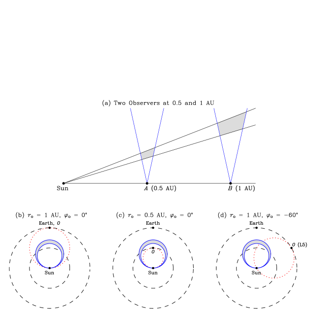
Figure 1.— Examples of the Thomson-scattering geometry for observers at different radial distances $r_{\rm o}$ and longitudes $\varphi_{\rm o}$. In panel (a), a radially-propagating solar wind parcel is viewed sequentially, but at the same scattering angle, by observers situated at radial distances of 0.5 AU (point $A$) and 1 AU (point $B$). Panels (b–d) illustrate the observation of an interplanetary sheath, denoted as a shaded region, by observers with different combinations of $r_{\rm o}$ and $\varphi_{\rm o}$. Longitude is defined to be positive (negative) for an observer situated to the west (east) of Earth.

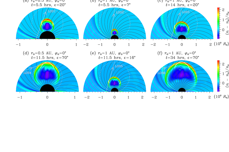
Figure 2.— Relative enhancement of electron number density, in the ecliptic, $(n-n_{0})/n_{0}$ within an Earth-directed interplanetary sheath. Red and black solid lines indicate sunward and anti-sunward interplanetary magnetic field lines, respectively. The sheath is imaged by two observers on the Sun-Earth line ($\varphi=0^{\circ}$), at heliocentric distances of $r_{\rm o}=0.5$ (left column) and 1 AU (central and right columns). For each observer, the ecliptic cross-section of its corresponding WL Thomson-scattering sphere is depicted as a dotted circle. Six lines-of-sight, LOS1–LOS6, are superimposed as straight arrows. All LOSs look westward. At any given time $t$, the two observers, both located on the Sun-Earth line, detect the sheath at different elongations $\varepsilon$ (compare panel a with panel b, and panel d with panel e). Conversely, when viewing along the same $\varepsilon$, the two observers detect the sheath at different $t$ (compare panel a with panel c, and panel d with panel f). Solid white curves overlaid on each panel indicate the position of the sheath inferred from polarised WL imaging.

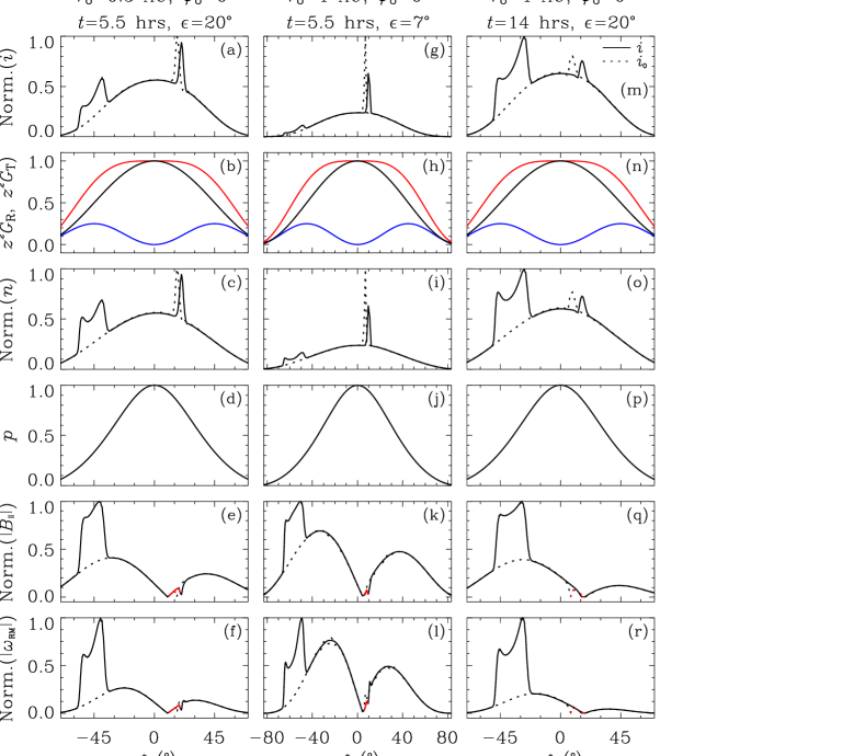
Figure 3.— WL radiance $i$, WL Thomson-scattering geometry factors ($z^{2}G$, $z^{2}G_{\rm R}$, $z^{2}G_{\rm T}$), electron number density $n$, degree of WL polarisation $p$, parallel magnetic field $|B_{\parallel}|$, and FR measurement $|\omega_{\rm RM}|$, plotted as a function of modified scattering angle $\chi^{*}=90-\chi$ along LOS1 (column A), LOS2 (column B), and LOS3 (column C). Each parameter is normalised to its maximum value along each LOS, as given in Table 1. Note that $i=n\,Z^{2}G$ and $\omega_{\rm RM}\propto n\,B_{\parallel}$. For the parameters $i$, $n$, $|B_{\parallel}|$, and $|\omega_{\rm RM}|$, initial and disturbed profiles are depicted as dashed and solid lines, respectively. The black and red sections of the $|B_{\parallel}|$ and $|\omega_{\rm RM}|$ profiles (two bottom rows) correspond to negative and positive values of $B_{\parallel}$, respectively.

Figure 4.— Dependence of the scattering angle $\chi^{*}$, the Thomson-scattering geometry factor $z^{2}G$, and the LOS depth $z$ on the degree of polarisation $p$ for LOS1 in Figure 2a. In response to shock passage, the initial radiance components, $I_{\rm T0}$ and $I_{\rm R0}$, are enhanced to values of $I_{\rm T}$ and $I_{\rm R}$, respectively. The enhancement in these radiance components determines the modified degree of polarisation $p^{*}$, according to the expression $p^{*}=\frac{I_{\rm T}-I_{\rm T0}-I_{\rm R}+I_{\rm R0}}{I-I_{0}}$. The vertical dashed line, demarking $p^{*}$, crosses the $\chi^{*}$ and $z$ profiles twice.

Figure 5.— The deviation of various parameters, from their initial values, plotted as a function of $z$ along LOS1. Note that $\frac{\delta\,(n\,B_{\parallel})}{\delta\,n}=\delta B_{\parallel}+B_{\parallel 0}+n_{0}\frac{\delta B_{\parallel}}{\delta n}=B_{\parallel}+n_{0}\frac{\delta B_{\parallel}}{\delta n}$. The parallel magnetic field component $B_{\parallel}^{*}$ (plotted as a horizontal dashed line in panel d) is calculated using the expression $\frac{\delta\,\Omega_{\rm RM}}{\delta\,I}=\frac{\int\delta\,\omega_{\rm RM}\,\,dz}{\int\delta\,i\,\,dz}=\frac{\int\delta\,(n\,B_{\parallel})\,\,dz}{\int z^{2}G\,\delta n\,\,dz}\approx\frac{1}{\,\,\overline{z^{2}G}\,\,}\,\frac{\delta\,(n\,B_{\parallel})}{\delta\,n}=\frac{1}{\,\,\overline{z^{2}G}\,\,}\,B_{\parallel}^{*}$.

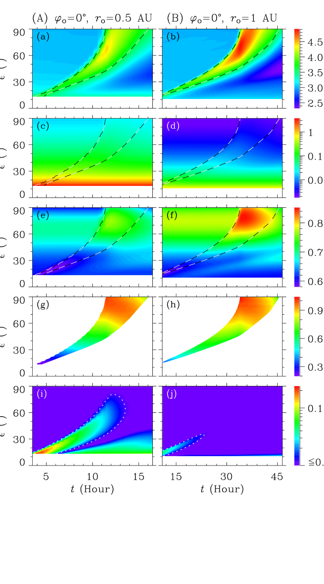
Figure 6.— Time-elongation maps of WL radiance (panels a and b: $I/I^{*}$, panels c and d: $I$), degree of WL polarisation (panels e and f: $p$, panels g and h: $p^{*}$), and FR measurement (panels i and j: $|\delta\,\Omega_{\rm RM}|$), as viewed by observers at longitude $\varphi_{\rm o}=0^{\circ}$ and at radii $r_{\rm o}=$ 0.5 AU (left column) and 1 AU (right column). $I^{*}$ is the normalisation factor for $I$, and corresponds to the radial variation of electron number density $n\propto r^{-2}$. The dotted lines in panels a–f correspond to $I/I^{*}=3.68\times 10^{-15}$. $p$ and $p^{*}$ are determined from the radiance and the enhancement in the radiance, respectively, as given by $p=\frac{I_{\rm T}-I_{\rm R}}{I}$ and $p^{*}=\frac{I_{\rm T}-I_{\rm T0}-I_{\rm R}+I_{\rm R0}}{I-I_{0}}$. Panels g and h only show $p^{*}$ within the sheath region.

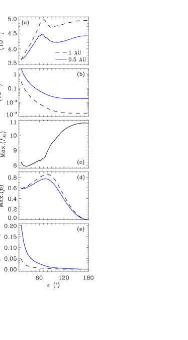
Figure 7.— A comparison of the WL radiance $I$ (panels a, b, and c), the degree of WL polarisation $p$ (panel d), and the FR measurement $\delta\,\Omega_{\rm RM}$ (panel e) over the elongation range from $15^{\circ}$ to $180^{\circ}$, as viewed by observers at 0.5 AU (solid line) and 1 AU (dashed line). The attribution “Max” refers to the strongest signal during the sheath passage.

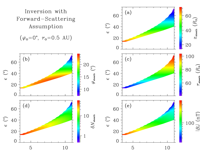
Figure 8.— Panels a–e present the location of the scattering site ($z_{\rm sheath}$, $\varphi_{\rm sheath}$, $r_{\rm sheath}$), the column-integrated electron number density $\delta N_{\rm sheath}$, and the parallel magnetic field $B_{\parallel}$, plotted as a function of time and elongation, derived by assuming forward-scattering ($\chi^{*}<0^{\circ}$).

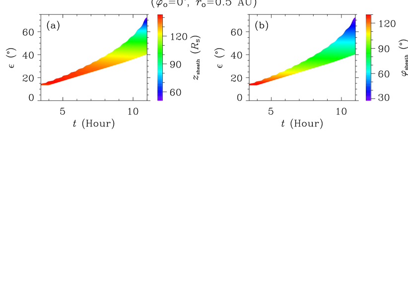
Figure 9.— Panels a–b present the location of the scattering site ($z_{\rm sheath}$, $\varphi_{\rm sheath}$), plotted as a function of time and elongation, derived by assuming backward-scattering ($\chi^{*}>0^{\circ}$).

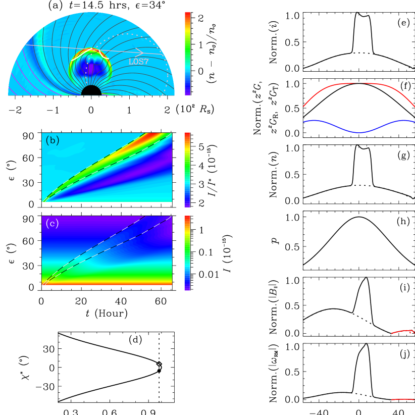
Figure 10.— Simulated results corresponding to the observation of an Earth-directed shock from the L5 vantage point, i.e., along LOS7 ($r_{\rm o}=1$ AU, $\varphi_{\rm o}=-60^{\circ}$): (panel a) relative enhancement of electron number density $(n-n_{0})/n_{0}$ in the ecliptic; (panels b and c) synthesised WL time-elongation maps of $I/I^{*}$ and $I$; (panel d) modified scattering angle $\chi^{*}$ as a function of the degree of polarisation $p$; (panels e–j) a number of synthesised WL and FR parameters, plotted as a function of $\chi^{*}$ along LOS7.

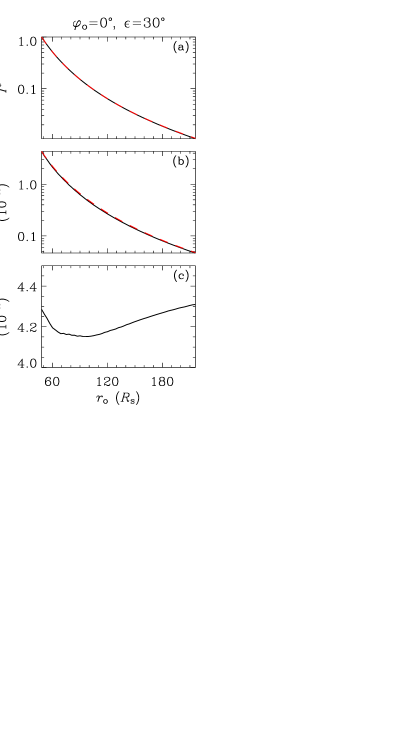
Figure 11.— Simulated WL radiance, as a function of $r_{\rm o}$, viewed along an elongation of $30^{\circ}$ by an observer on the Sun-Earth line ($\varphi_{\rm o}=0^{\circ}$, $50\,R_{\rm S}\leq r\leq 215\,R_{\rm S}$). Again, “Max” refers to the strongest signal associated with the sheath passage. The dashed red lines in the two upper panels show, for comparison, an $r^{-3}$ variation. Both $I^{*}$ and $\mbox{Max.}(I)$ are well described by such a variation.

Table 1Maximum values of the parameters $i$, $z^{2}G$, $z^{2}G_{\rm R}$, $z^{2}G_{\rm T}$, $n$, $|B_{\parallel}|$, and $|\omega_{\rm RM}|$ along LOS1, LOS2, LOS3, and LOS7, used for normalisation in Figures 3 and 10e-j. Each LOS is designated a time $t$, a radius $r_{\rm o}$, a longitude $\varphi_{\rm o}$, and an elongation $\varepsilon$ in columns 2-5; LOSs 1-6 are overlaid on Figure 2 and LOS7 is overlaid on Figure 10.

LOS	Time	Radii	Longitude	Elongation	WL radiance	WL Thomson-scattering	Electron	Parallel magnetic	FR measurement
	$t$	$r_{\rm o}$	$\varphi_{\rm o}$	$\varepsilon$	$i$	geometry factors	number	field
	(hour)	(AU)	(∘)	(∘)	($\times 10^{-27}$)	$z^{2}G$, $z^{2}G_{\rm R}$, $z^{2}G_{\rm T}$	density $n$	$|B_{\parallel}|$	$|\omega_{\rm RM}|$
						($\times 10^{-29}$)	(cm-3)	(nT)	($\times 10^{-12}$ rad m-3)
LOS1	5.5	0.5	0	20	36.3	9.33	392	207	14.4
LOS2	5.5	1	0	7	344	18.2	1893	223	18.2
LOS3	14	1	0	20	1.93	2.31	87	68.9	1.51
LOS7	14.5	1	-60	34	0.52	0.86	60.3	28.5	0.42

References

- Akioka et al. (2005) Akioka, M., Nagatsuma, T., Miyake, W., Ohtaka, K., & Marubashi, K. 2005, Advances in Space Research, 35, 65
- Bemporad et al. (2012) Bemporad, A., Zuccarello, F. P., Jacobs, C., Mierla, M., & Poedts, S. 2012, Sol. Phys., 281, 223
- Biesecker et al. (2008) Biesecker, D. A., Webb, D., & St. Cyr, O. 2008, Space Sci. Rev., 136, 45
- Billings (1966) Billings, D. E. 1966, A Guide to the Solar Corona (San Diego: Academic Press)
- Bird et al. (1980) Bird, M. K., Schrüfer, E., Volland, H., & Sieber, W. 1980, Nature, 283, 459
- Bird et al. (1985) Bird, M. K., Volland, H., Howard, R. A., et al. 1985, Sol. Phys., 98, 341
- Bisi et al. (2008) Bisi, M. M., Jackson, B. V., Hick, P. P., et al. 2008, J. Geophys. Res., 113, A00A11
- Burlaga et al. (1987) Burlaga, L. F., Behannon, K. W., & Klein, L. W. 1987, J. Geophys. Res., 92, 5725
- Burlaga et al. (2002) Burlaga, L. F., Plunkett, S. P., & Cyr, O. C. S. 2002, J. Geophys. Res., 107
- Burlaga et al. (1981) Burlaga, L. F., Sittler, E., Mariani, F., & Schwenn, R. 1981, J. Geophys. Res., 86, 6673
- Cargill (2004) Cargill, P. J. 2004, Sol. Phys., 221, 135
- Cargill et al. (1996) Cargill, P. J., Chen, J., Spicer, D. S., & Zalesak, S. T. 1996, J. Geophys. Res., 101, 4855
- Chen (1989) Chen, J. 1989, ApJ, 338, 453
- Chen (1996) —. 1996, J. Geophys. Res., 101, 27499
- Chen et al. (2006) Chen, Y., Li, G. Q., & Hu, Y. Q. 2006, ApJ, 649, 1093
- Crifo et al. (1983) Crifo, F., Picat, J. P., & Cailloux, M. 1983, Sol. Phys., 83, 143
- Crooker et al. (2004) Crooker, N. U., Huang, C. L., Lamassa, S. M., et al. 2004, J. Geophys. Res., 109, A03107
- Davies et al. (2009) Davies, J. A., Harrison, R. A., Rouillard, A. P., et al. 2009, Geophys. Res. Lett., 36, L02102
- Davies et al. (2012) Davies, J. A., Harrison, R. A., Perry, C. H., et al. 2012, ApJ, 750, 23
- Davis et al. (2009) Davis, C. J., Davies, J. A., Lockwood, M., et al. 2009, Geophys. Res. Lett., 36, L08102
- Davis et al. (2010) Davis, C. J., Kennedy, J., & Davies, J. A. 2010, Sol. Phys., 263, 209
- de Koning et al. (2009) de Koning, C. A., Pizzo, V. J., & Biesecker, D. A. 2009, Sol. Phys., 256, 167
- de Vos et al. (2009) de Vos, M., Gunst, A. W., & Nijboer, R. 2009, IEEE Proc., 97, 1431
- DeForest et al. (2011) DeForest, C., Howard, T., & Tappin, S. 2011, ApJ, 738, 103
- DeForest et al. (2013) DeForest, C. E., Howard, T. A., & Tappin, S. J. 2013, ApJ, 765, 44
- Démoulin (2010) Démoulin, P. 2010, in 12th International Solar Wind Conference, ed. M. Maksimovic, K. Issautier, N. Meyer-Vernet, M. Moncuquet, & F. Pantellini, Vol. 1216 (AIP Conference Proceedings), 329
- Démoulin & Dasso (2009) Démoulin, P., & Dasso, S. 2009, A&A, 498, 551
- Démoulin et al. (2013) Démoulin, P., Dasso, S., & Janvier, M. 2013, A&A, 550, A3
- Echer et al. (2004) Echer, E., Alves, M. V., & Gonzalez, W. D. 2004, Sol. Phys., 221
- Eyles et al. (2003) Eyles, C. J., Simnett, G. M., Cooke, M. P., et al. 2003, Sol. Phys., 217, 319
- Eyles et al. (2009) Eyles, C. J., Harrison, R. A., Davis, C. J., et al. 2009, Sol. Phys., 254, 387
- Farrugia et al. (1993) Farrugia, C. J., Burlaga, L. F., Osherovich, V. A., & et al. 1993, J. Geophys. Res., 98, 7621
- Feng et al. (2012a) Feng, L., Inhester, B., Wei, Y., et al. 2012a, ApJ, 751, 18
- Feng et al. (2012b) Feng, X., Jiang, C., Xiang, C., Zhao, X., & Wu, S. T. 2012b, ApJ, 758, 62
- Goldshmidt & Rephaeli (1993) Goldshmidt, O., & Rephaeli, Y. 1993, ApJ, 411, 518
- Gómez et al. (2008) Gómez, J., Marscher, A. P., Jorstad, S. G., Agudo, I., & Roca-Sogorb, M. 2008, ApJ, 681, L69
- Gonzalez et al. (1999) Gonzalez, W., Tsurutani, B., & Gonzalez, C. D. 1999, Space Sci. Rev., 88, 529
- Gopalswamy (2006) Gopalswamy, N. 2006, Space Sci. Rev., 124, 145
- Gopalswamy et al. (2001) Gopalswamy, N., Yashiro, S., Kaiser, M. L., Howard, R. A., & Bougeret, J. L. 2001, ApJ, 548, L91
- Gopalswamy et al. (2011) Gopalswamy, N., Davila, J. M., St. Cyr, O. C., et al. 2011, J. Atmos. Sol. Terr. Phys., 73, 658
- Gosling & McComas (1987) Gosling, J. T., & McComas, D. J. 1987, Geophys. Res. Lett., 14, 355
- Gosling & Pizzo (1999) Gosling, J. T., & Pizzo, V. J. 1999, Space Sci. Rev., 89, 21
- Groth et al. (2000) Groth, C. P. T., De Zeeuw, D. L., Gombosi, T. I., & Powell, K. G. 2000, J. Geophys. Res., 105, 25053
- Gulisano et al. (2012) Gulisano, A. M., Démoulin, P., Dasso, S., & Rodriguez, L. 2012, A&A, 543, A107
- Gulisano et al. (2010) Gulisano, A. M., Démoulin, P., Dasso, S., Ruiz, M. E., & Marsch, E. 2010, A&A, 509, A39
- Harrison et al. (2009) Harrison, R. A., Davies, J. A., & Rouillard, A. P. 2009, Sol. Phys., 256, 219
- Harrison et al. (2008) Harrison, R. A., Davis, C. J., Eyles, C. J., et al. 2008, Sol. Phys., 247, 171
- Harrison et al. (2012) Harrison, R. A., Davies, J. A., Möstl, C., et al. 2012, ApJ, 750, 45
- Hayashi (2005) Hayashi, K. 2005, Astrophys. J. Suppl. Ser., 161, 480
- Hollweg et al. (2010) Hollweg, J. V., Cranmer, S. R., & Chandran, B. D. G. 2010, ApJ, 722, 1495
- Howard & DeForest (2012) Howard, T. A., & DeForest, C. E. 2012, ApJ, 752, 130
- Howard & Tappin (2009) Howard, T. A., & Tappin, S. J. 2009, Space Sci. Rev., 147, 31
- Howard et al. (2013) Howard, T. A., Tappin, S. J., Odstrcil, D., & DeForest, C. E. 2013, ApJ, 765, 45
- Hu & Sonnerup (2002) Hu, Q., & Sonnerup, B. U. Ö. 2002, J. Geophys. Res., 107, 1142
- Hu & Jia (2001) Hu, Y. Q., & Jia, X. Z. 2001, J. Geophys. Res., 106, 29,299
- Jackson et al. (2010) Jackson, B., Buffington, A., Hick, P., Bisi, M., & Clover, J. 2010, Sol. Phys., 265, 257
- Jackson et al. (2006) Jackson, B. V., Buffington, A., Hick, P. P., & Webb, D. F. 2006, J. Geophys. Res., 111
- Jensen (2007) Jensen, E. A. 2007, High frequency Faraday rotation observations of the solar corona (Ph.D. Dissertation), University of California, Los Angeles, USA
- Jensen et al. (2010) Jensen, E. A., Hick, P. P., Bisi, M. M., et al. 2010, Sol. Phys., 265, 31
- Jensen et al. (2013) Jensen, E. A., Nolan, M., Bisi, M. M., Chashei, I., & Vilas, F. 2013, Sol. Phys., 285, 71
- Jensen & Russell (2008) Jensen, E. A., & Russell, C. T. 2008, Geophys. Res. Lett., 35, L02103
- Jokipii & Lerche (1969) Jokipii, J. R., & Lerche, I. 1969, ApJ, 157, 1137
- Klein & Burlaga (1982) Klein, L. W., & Burlaga, L. F. 1982, J. Geophys. Res., 87, 613
- Leinert & Pitz (1989) Leinert, C., & Pitz, E. 1989, A&A, 210, 399
- Lepping et al. (1990) Lepping, R. P., Burlaga, L. F., & Jones, J. A. 1990, J. Geophys. Res., 95, 11957
- Levy et al. (1969) Levy, G., Sato, T., Seidel, B. L., et al. 1969, Science, 166, 596
- Li & Li (2008) Li, B., & Li, X. 2008, ApJ, 682, 667
- Li et al. (2006) Li, B., Li, X., & Labrosse, N. 2006, J. Geophys. Res., 111, A08106
- Liu et al. (2010b) Liu, Y., Davies, J. A., Luhmann, J. G., et al. 2010b, ApJ, 710, L82
- Liu et al. (2013) Liu, Y., Luhmann, J. G., Lugaz, N., et al. 2013, ApJ, 769
- Liu et al. (2007) Liu, Y., Manchester IV, W. B., Kasper, J. C., Richardson, J. D., & Belcher, J. W. 2007, ApJ, 665, 1439
- Liu et al. (2008) Liu, Y., Manchester IV, W. B., Richardson, J. D., et al. 2008, J. Geophys. Res., 113, A00B03
- Liu et al. (2012) Liu, Y., Luhmann, J. G., Möstl, C., et al. 2012, ApJ, 746
- Lonsdale, C. J., et. al. (2009) Lonsdale, C. J., et. al. 2009, IEEE Proc., 97, 1497
- Lugaz et al. (2012) Lugaz, N., Farrugia, C. J., Davies, J. A., et al. 2012, ApJ, 759, 68
- Lugaz et al. (2010) Lugaz, N., Hernandez-Charpak, J. N., Roussev, I. I., et al. 2010, ApJ, 715, 493
- Lugaz & Kintner (2013) Lugaz, N., & Kintner, P. 2013, Sol. Phys., 285, 281
- Lugaz et al. (2005) Lugaz, N., Manchester IV, W. B., & Gombosi, T. I. 2005, ApJ, 634, 651
- McComas et al. (2000) McComas, D. J., Barraclough, B., Funsten, H., et al. 2000, J. Geophys. Res., 105, 10419
- Moran & Davila (2004) Moran, T. G., & Davila, J. M. 2004, Science, 305, 66
- Moran et al. (2010) Moran, T. G., Davila, J. M., & Thompson, W. T. 2010, ApJ, 712, 453
- Möstl & Davies (2013) Möstl, C., & Davies, J. A. 2013, Sol. Phys., 285, 411
- Möstl et al. (2011) Möstl, C., Rollett, T., Lugaz, N., et al. 2011, ApJ, 741
- Möstl et al. (2012) Möstl, C., Farrugia, C. J., Kilpua, E. K. J., et al. 2012, ApJ, 758
- Nakwacki et al. (2011) Nakwacki, M. S., Dasso, S., Démoulin, P., Mandrini, C. H., & Gulisano, A. M. 2011, A&A, 535
- Oberoi & Lonsdale (2012) Oberoi, D., & Lonsdale, C. J. 2012, Radio Science, 47, RS0K08
- Odstrčil & Pizzo (2009) Odstrčil, D., & Pizzo, V. J. 2009, Sol. Phys., 259, 297
- Odstrčil et al. (1996) Odstrčil, D., Smith, Z., & Dryer, M. 1996, Geophys. Res. Lett., 23, 2521
- Oliveros et al. (2012) Oliveros, J. C. M., Raftery, C. L., Bain, H. M., et al. 2012, ApJ, 748, 66
- Owens et al. (2005) Owens, M., Cargill, P., Pagel, C., Siscoe, G., & Crooker, N. 2005, J. Geophys. Res., 110, A01105
- Parker (1958) Parker, E. N. 1958, ApJ, 128, 664
- Pätzold & Bird (1998) Pätzold, M., & Bird, M. K. 1998, Geophys. Res. Lett., 25, 2105
- Pizzo & Biesecker (2004) Pizzo, V. J., & Biesecker, D. A. 2004, Geophys. Res. Lett., 31, L21802
- Plunkett et al. (1998) Plunkett, S. P., Thompson, B. J., Howard, R. A., et al. 1998, Geophys. Res. Lett., 25, 2477
- Poland & Munro (1976) Poland, A. I., & Munro, R. H. 1976, ApJ, 209, 927
- Reichstein & Gabuzda (2012) Reichstein, A., & Gabuzda, D. 2012, Journal of Physics: Conference Series 355; International Workshop on Beamed and Unbeamed Gamma-Rays from Galaxies, 012021
- Rouillard et al. (2008) Rouillard, A. P., Davies, J. A., Forsyth, R. J., et al. 2008, Geophys. Res. Lett., 35, L10110
- Rouillard et al. (2009a) Rouillard, A. P., Savani, N. P., Davies, J. A., et al. 2009a, Sol. Phys., 256, 307
- Rouillard et al. (2009b) Rouillard, A. P., Davies, J. A., Forsyth, R. J., et al. 2009b, J. Geophys. Res., 114, A07106
- Sakurai & Spangler (1994) Sakurai, T., & Spangler, S. R. 1994, ApJ, 434, 773
- Savani et al. (2010) Savani, N. P., Owens, M. J., Rouillard, A. P., Forsyth, R. J., & Davies, J. A. 2010, ApJ, 714, L128 CL132
- Savani et al. (2012) Savani, N. P., Davies, J. A., Davis, C. J., et al. 2012, Sol. Phys., 279, 517
- Sheeley et al. (2008) Sheeley, N. R., J., Herbst, A. D., Palatchi, C. A., et al. 2008, ApJ, 674, 109
- Shen et al. (2012a) Shen, C., Wang, Y., Wang, S., et al. 2012a, Nature Physics, 8, 923
- Shen et al. (2012b) Shen, F., Wu, S. T., Feng, X. S., & Wu, C. C. 2012b, J. Geophys. Res., 117, A11101
- Steed et al. (2011) Steed, K., Owen, C. J., Démoulin, P., & Dasso, S. 2011, J. Geophys. Res., 116, A01106
- Szajko et al. (2013) Szajko, N., Cristiani, G., Mandrini, C., & Dal Lago, A. 2013, Advances in Space Research, 51, 1842
- Tappin et al. (2004) Tappin, S. J., Buffington, A., Cooke, M. P., et al. 2004, Geophys. Res. Lett., 31, L02802
- Temmer et al. (2011) Temmer, M., Rollett, T., Möstl, C., et al. 2011, ApJ, 743, 101
- Temmer et al. (2012) Temmer, M., Vršnak, B., Rollett, T., et al. 2012, ApJ, 749, 57
- Thernisien et al. (2009) Thernisien, A., Vourlidas, A., & Howard, R. A. 2009, Sol. Phys., 256, 111
- Thompson et al. (1980) Thompson, A. R., Clark, B. G., Wade, C. M., & Napier, P. J. 1980, Astrophysical Journal Supplement Series, 44, 151
- Thompson et al. (1998) Thompson, B. J., Plunkett, S. P., Gurman, J. B., et al. 1998, Geophys. Res. Lett., 25, 2465
- Tsurutani et al. (1992) Tsurutani, B. T., Lee, Y. T., Gonzalez, W. D., & Tang, F. 1992, Geophys. Res. Lett., 19, 73
- Tsurutani et al. (1988) Tsurutani, B. T., Smith, E. J., Gonzalez, W. D., Tang, F., & Akasofu, S. I. 1988, J. Geophys. Res., 93, 8519
- Vourlidas & Howard (2006) Vourlidas, A., & Howard, R. A. 2006, ApJ, 642, 1216
- Vršnak & Gopalswamy (2002) Vršnak, B., & Gopalswamy, N. 2002, J. Geophys. Res., 107, SSH 2
- Wang et al. (2003a) Wang, Y. M., Ye, P. Z., & Wang, S. 2003a, J. Geophys. Res., 108, 1370
- Webb & Howard (2012) Webb, D. F., & Howard, T. A. 2012, Living Reviews in Solar Physics, 9
- Webb et al. (2013) Webb, D. F., Möstl, C., Jackson, B. V., et al. 2013, Sol. Phys., 285, 317
- Winterhalter et al. (1994) Winterhalter, D., Smith, E. J., Burton, M. E., Murphy, N., & McComas, D. J. 1994, J. Geophys. Res., 99, 6667
- Woo (1997) Woo, R. 1997, Geophys. Res. Lett., 24, 97
- Wu et al. (2006) Wu, S. T., Wang, A. H., Liu, Y., & Hoeksema, J. T. 2006, ApJ, 652, 800
- Xiong et al. (2011) Xiong, M., Breen, A., Bisi, M., et al. 2011, J. Atmos. Sol. Terr. Phys., 73, 1270
- Xiong et al. (2013) Xiong, M., Davies, J. A., Bisi, M. M., et al. 2013, Sol. Phys., 285, 369
- Xiong et al. (2009) Xiong, M., Zheng, H. N., & Wang, S. 2009, J. Geophys. Res., 114
- Xiong et al. (2006a) Xiong, M., Zheng, H. N., Wang, Y. M., & Wang, S. 2006a, J. Geophys. Res., 111
- Xiong et al. (2006b) —. 2006b, J. Geophys. Res., 111
- Xiong et al. (2007) Xiong, M., Zheng, H. N., Wu, S. T., Wang, Y. M., & Wang, S. 2007, J. Geophys. Res., 112
- You et al. (2012) You, X. P., Coles, W. A., Hobbs, G. B., & Manchester, R. N. 2012, MNRAS, 422, 1160
- Zavala & Taylor (2002) Zavala, R. T., & Taylor, G. B. 2002, ApJ, 566, L9
- Zhang et al. (2008) Zhang, J., Richardson, I. G., & Webb, D. F. 2008, J. Geophys. Res., 113, A00A12
- Zhang et al. (2013) Zhang, Y., Du, A. M., Sun, W., et al. 2013, Sol. Phys., accepted