Hole propagation in the Kitaev-Heisenberg model:
From quasiparticles in quantum Néel states to non-Fermi liquid in the Kitaev phase

Abstract

We explore with exact diagonalization the propagation of a single hole in four magnetic phases of the $t$-$J$-like Kitaev-Heisenberg model on a honeycomb lattice: the Néel antiferromagnetic, stripe, zigzag and Kitaev spin-liquid phase. We find coherent propagation of spin-polaron quasiparticles in the antiferromagnetic phase by a similar mechanism as in the $t$-$J$ model for high-$T_{c}$ cuprates. In the stripe and zigzag phases clear quasiparticles features appear in spectral functions of those propagators where holes are created and annihilated on one sublattice, while they remain largely hidden in those spectral functions that correspond to photoemission experiments. As the most surprising result, we find a totally incoherent spectral weight distribution for the spectral function of a hole moving in the Kitaev spin-liquid phase in the strong coupling regime relevant for iridates. At intermediate coupling the finite systems calculation reveals a well defined quasiparticle at the $\Gamma$ point, however, we find that the gapless spin excitations wipe out quasiparticles at finite momenta. Also for this more subtle case we conclude that in the thermodynamic limit the lightly doped Kitaev liquid phase does not support quasiparticle states in the neighborhood of $\Gamma$, and therefore yields a non-Fermi liquid, contrary to earlier suggestions based on slave-boson studies. These observations are supported by the presented study of the dynamic spin-structure factor for the Kitaev spin liquid regime.

I Introduction

Carrier propagation in Mott or charge-transfer insulators is a challenging problem particularly motivated by strongly correlated superconducting cuprates Dag94 ; Szc90 ; Eme97 ; Lee06 . While holes move incoherently in one-dimensional systems featuring charge and spin separation And90 as well as in systems with antiferromagnetic (AF) Ising interactions Bri70 ; Tru88 , the hole motion becomes coherent and quasiparticles (QPs) arise at low energy in the quantum AF $t$-$J$ model Mar91 . These QPs are indeed observed in angle-resolved photoemission (ARPES) experiments in cuprates And03 . In general, low-energy QPs coexist with incoherent processes at high energy, as in the AF phase on the square Mar91 or honeycomb lattice Sus06 . This is however not always the case as shown by ARPES experiments for the spin-orbit Mott insulator Na₂IrO₃ Com12 , without clear evidence for QPs at low energy Tro13 . In a recent study hole-doped Li₂Ir_1-xRu_xO₃ with honeycomb structure was found insulating at all doping levels Lei13 .

Electronic systems with honeycomb lattice include graphene Gra09 ; Pol13 , optical lattices Wun08 , topological insulators Hoh13 , and frustrated magnets Nor09 ; Bal10 ; Kit06 ; Nus13 ; Jac09 ; Mur10 ; Cha10 ; Tre11 . Interest in the latter was triggered by theoretical predictions Jac09 ; Shi09 that Na₂IrO₃ may host Kitaev model physics and quantum spin Hall effect. The ground state of this model is a Kitaev spin liquid (KSL) characterized by finite spin correlations only for nearest neighbor (NN) spins Bas07 . The KSL belongs to the spin disordered phases which are in the center of interest in quantum magnetism Nor09 ; Bal10 . In Mott insulators where the strong spin-orbit interaction generates a Kramers doublet from partly filled $t_{2g}$ orbitals Jac09 ; Cha10 , as in Na₂IrO₃, effective $S=1/2$ pseudospins stand for local, spin-orbital entangled $t_{2g}$ states which form orbital moments Hor03 . Both Kitaev and Heisenberg interactions emerge from the spin and orbital coupling on the honeycomb lattice of iridium ions and form the Kitaev-Heisenberg (KH) model Jac09 . Experimental observations revealed zigzag (ZZ) magnetic order in Na₂IrO₃ Liu11 ; Sin12 ; Ye12 — it may be explained within the KH model with next-nearest neighbor (NNN) $J_{2}$ and third NN (3NN) $J_{3}$ AF interactions Cha10 ; Tre11 . The phase diagram of the frustrated Heisenberg $J_{1}$-$J_{2}$-$J_{3}$ AF model Alb11 ; Gan13 includes the Néel AF, ZZ, and also stripy (ST) phase. These phases survive when more general spin interactions with symmetric off-diagonal exchange are considered Rau14 .

Doping the KSL is particularly exciting as the ground state is spin disordered and it is unclear whether QPs would form Sen03 . Moreover in the KSL interactions may emerge that lead to unexpected forms of superconductivity. Indeed, slave-boson studies found here $p$-wave superconductivity at intermediate doping Hya12 ; You12 ; Oka13 ; Bur11 , whereas Fermi liquid was claimed at light doping Mei12 . An important first step to explore hole doping is however the study of single hole motion and the existence of QPs. So far, spin-charge separation was shown for the kagome lattice, being a prototype of a spin liquid, while small QP peaks were found at some momenta in a frustrated checkerboard lattice Lau04 . The $t$-$J$-like KH model provides here a unique opportunity to investigate hole propagation in quite different magnetic phases emerging from frustrated interactions.

The purpose of this paper is: (i) to investigate the evolution of the spectral properties in the KH model under increasing frustration of magnetic interactions, (ii) to recognize the QP behavior in various magnetic phases of the frustrated KH model, and (iii) to establish whether the disordered KSL indeed realizes a paradigm of a Fermi liquid at light doping as suggested in Ref. Mei12 . In our study we employ exact diagonalization (ED) of finite periodic clusters which has the important advantage that no approximations have to be made, which is particularly important as the analytical theory of hole-motion in the KH model is notoriously difficult and largely unexplored. The possible problems with the ED approach are finite size effects and the difficulty to extrapolate to the thermodynamic limit (TL). As important results, we report the spectral functions of the different ordered phases and their respective quasiparticle features. Moreover we report a totally incoherent spectral weight distribution for a hole moving in the Kitaev spin-liquid phase in the strong coupling regime, i.e., relevant for the iridate systems. The absence of QPs in this case for finite systems clearly suggests that also in the TL there are no QPs at strong coupling. For this reason we conclude that then a dilute gas of holes (that are individually not QPs) will not turn into a Fermi liquid.

The paper is organized as follows: In the Sect. II we outline the KH model and discuss the calculation of various correlation functions that are used to determine the phase diagram of the KH-model. Section III deals with the motion of holes in the ordered phases of the model and discusses the different propagators and spectral functions used. In Sect. IV we address the hole motion in the KSL and analyse the spectral weight distribution. The latter is discussed in the intermediate and strong coupling limit. Moreover the dynamical spin structure factor is analysed for the KSL both for the Kitaev and the KH model in order to explore the different scattering channels for holes. Results are summarized in Sect. V.

II The Kitaev-Heisenberg Model

II.1 Frustrated spin interactions
and exact diagonalization

We consider the following $t$-$J$-like KH model ($t>0$), on the honeycomb lattice [Fig. 1(a)]:

$${\cal H}_{tJ} \,\equiv t\sum_{\langle ij\rangle\sigma}c^{\dagger}_{i\sigma}c_{j\sigma}+J_{K}\sum_{\langle ij\rangle\parallel\gamma}S_{i}^{\gamma}S_{j}^{\gamma}+J_{1}\sum_{\langle ij\rangle}\vec{S}_{i}\!\cdot\!\vec{S}_{j}$$ (1)

$$+ \!(1-\alpha)\,\Big{\{}J_{2}\!\!\sum_{\{ij\}\in{\rm NNN}}\!\!\vec{S}_{i}\!\cdot\!\vec{S}_{j}+J_{3}\!\!\sum_{\{ij\}\in{\rm 3NN}}\!\!\vec{S}_{i}\cdot\vec{S}_{j}\Big{\}}\,,$$

It consists of the kinetic energy term $\propto t$ of projected fermions with flavor $\sigma$ Tro13 ; Hya12 ; You12 which move in the restricted space without double occupancies as a result of large on-site Coulomb repulsion $U$. The spins $S=1/2$ are defined in terms of fermionic creation (annihilation) operators $c^{\dagger}_{i\sigma}$ ($c_{i\sigma}$) with flavor $\sigma$ at site $i$:

$$S_{i}^{\gamma}\equiv\frac{1}{2}\;c^{\dagger}_{i\sigma}\tau^{\gamma}_{\sigma\sigma^{\prime}}c_{i\sigma^{\prime}},$$ (2)

where $\tau^{\gamma}_{\sigma\sigma^{\prime}}$ are Pauli matrices, $\gamma=\{x,y,z\}$. We emphasize that already the Kitaev terms $\propto J_{K}$ with different Ising spin interactions that depend on bond direction introduce strong spin frustration in Eq. (1). In the following we shall assume ferromagnetic (FM) Kitaev ($J_{K}<0$) and AF Heisenberg ($J_{1}>0$) exchange,

$$J_{K}\equiv-2J\alpha\,,\hskip 19.91684ptJ_{1}\equiv J(1-\alpha)\,.$$ (3)

Here $J$ is the energy unit and $\alpha\!\in\![0,1]$ is a parameter that interpolates between the Heisenberg and Kitaev exchange couplings for NN spins $S=1/2$. The model Eq. (1) includes NNN $\propto J_{2}$ and 3NN $\propto J_{3}$ AF terms as well.

We use exact diagonalization (ED) within the Lanczos algorithm for a periodic cluster of $N=24$ sites which accomodates all point group symmetries of the infinite lattice. The momenta corresponding to allowed symmetry representations are presented in the first Brillouin zone (BZ) in Fig. 1(b). We introduce $M_{z}=(0,2\pi/\sqrt{3})$, $M_{x/y}=(\pi,\pm\pi/\sqrt{3})$, and $\pm P_{\gamma}$, where $M_{\gamma}\perp P_{\gamma}$ and $2P_{\gamma}\equiv K_{\gamma}$. Note that in absence of symmetry-breaking field, $K_{z}$ and $-K_{y}$ are identical and only two distinct representations exist, $\pm K_{z}$.

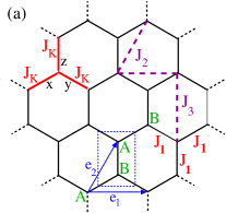
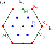
Figure 1: (Color online) (a) Periodic cluster of the honeycomb lattice (solid and dashed bonds) with $N=24$ sites and the elementary translations $\vec{e}_{1(2)}$ that connect atoms $A$ within one sublattice, i.e., connect unit cells consisting of one atom $A$ and one $B$ each. Heisenberg couplings between NN ($J_{1}$), NNN ($J_{2}$) and 3NN ($J_{3}$) in ${\cal H}_{tJ}$ (1) are indicated by solid and dashed lines; Kitaev couplings $J_{K}$ involve a single spin component for each bond direction, $\gamma\in\{x,y,z\}$. (b) First BZ with high symmetry $M_{\gamma}$ and $K_{\gamma}$ points (in absence of symmetry breaking these points are equivalent to one another).

II.2 Phase diagram

In the present ED approach of finite systems there is no spontaneous symmetry breaking, and the spin components $x$, $y$, and $z$ are equivalent. The intrinsic spin order parameter ${\cal S}_{\Phi}$ in the ground state can be determined by identifying and calculating the respective correlation functions that reflect the emerging long-range order Kap89 ; Kom94 ,

$${\cal S}_{\Phi}^{2}\equiv{\frac{12}{N^{2}}\sum_{i,j=1}^{N/2}e^{i\vec{k}\cdot\vec{R}_{ij}}\langle(S^{z}_{iA}\pm S^{z}_{iB})(S^{z}_{jA}\pm S^{z}_{jB})\rangle}\,,$$ (4)

for each phase $\Phi$, where $\langle\dots\rangle\equiv\langle 0|\dots|0\rangle$ is the average over the ground state $|0\rangle$. In this definition we select $"-"$ sign for the spin components $S_{jB}^{z}$ for the Néel AF phase and $"+"$ sign for the staggered and ZZ phase; $\vec{k}=\Gamma$ for the Néel ($\Phi={\rm AF}$), $\vec{k}=M_{z}$ for the ST ($\Phi={\rm ST}$), and either $\vec{k}=M_{x}$ or $\vec{k}=M_{y}$ for the ZZ ($\Phi={\rm ZZ}$) phase (these points are equivalent in this case). Here $i$ and $j$ label unit cells [Fig. 1(a)], and $\vec{R}_{ij}=\vec{r}_{i}-\vec{r}_{j}$. The order parameter ${\cal S}_{\Phi}$ (4) is large when spin correlations are close to the ones expected for a magnetic phase $\Phi$; in all other phases it is negligible. Two examples are shown in Fig. 2(a): (i) for $\alpha<0.5$ one finds large ${\cal S}_{\rm AF}\simeq 1$, and (ii) for $0.5<\alpha<0.85$ this order parameter drops to ${\cal S}_{\rm AF}\ll 1$ but ${\cal S}_{\rm ZZ}$ increases to ${\cal S}_{\rm ZZ}>0.6$. Indeed, a transition between the AF and ZZ phase is found here, see dotted line in Fig. 2(b), while the ST phase is unstable here and ${\cal S}_{\rm ST}$ is small.

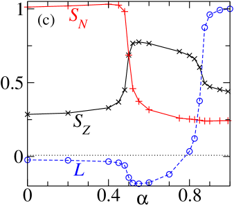
Figure 2: (Color online) (a) Order parameters ${\cal S}_{\Phi}$ (4) representing the Néel ($\Phi$=AF), the zigzag ($\Phi$=ZZ) and the Kitaev invariant ${\cal L}$ (5) obtained for $J_{2}=0$ and $J_{3}=0.4J$. (b) Phase diagram of the KH model Eq. (1) in $(\alpha,J_{3}/J)$ plane (points) for $J_{2}=0$, with AF, ST, ZZ and KSL phases The insets show types of magnetic order (arrows) or disorder (circles).

In the KSL phase spin correlations $\langle S^{\gamma}_{i}S^{\gamma}_{j}\rangle$ vanish beyond NN spins at $\alpha=1$ Kit06 ; Bas07 ; Tro11 , and further neighbor correlations remain small in the Kitaev liquid regime at $\alpha\neq 1$ Tro11 . This results in ${\cal S}_{\rm\Phi}\ll 1$ for all conventional spin order parameters SKl . To identify the KSL we introduce here an average of the Kitaev invariant Kit06 on a single hexagon ${\cal C}_{6}$,

$${\cal L}\equiv 2^{6}\left\langle\prod_{i\in{\cal C}_{6}}S^{\gamma}_{i}\right\rangle,$$ (5)

where $\gamma$ labels the spin component $S^{\gamma}_{i}$ interacting with a spin at site $j$ along the outgoing bond $\langle ij\rangle\notin{\cal C}_{6}$ via $J_{K}S^{\gamma}_{i}S^{\gamma}_{j}$. One finds that ${\cal L}\to 1$ when the ground state of the Kitaev model is approached at $\alpha\to 1$, see Fig. 2(a).

The phase diagram in the $J_{3}$ versus $\alpha$ plane is displayed in Fig. 2(b). We recognize the AF phase at small $\alpha$, the intermediate ST phase, and at large $\alpha>0.8$ — the Kitaev liquid phase. At large further neighbor exchange interaction $J_{3}$ the zigzag phase emerges in the intermediate range of $\alpha$. Theses phases were identified by the order parameters discussed above, while the phase boundaries were determined by a different powerful tool, namely the study of the fidelity susceptibility You07 ; Gu10 , i.e., the changing rate of the overlap between ground states at adjacent points. Note that the AF$\leftrightarrow$ZZ transition at $\alpha=0.5$ follows from symmetry arguments and as such is independent of the cluster size.

III Carrier propagation in quantum antiferromagnetic phases

In the following we shall analyze the spectral properties of a hole inserted into the ordered ground state $|0\rangle$, being the quantum Néel AF, ST, or ZZ phase. The KSL phase will be explored in detail in the subsequent Section. We use here the standard numerical Lanczos algorithm which spans efficiently the relevant Krylov space and yields spectral functions in form of a continued fraction Szc90 ; Gb87 . The calculation begins with the determination of the ground state $|0\rangle$ and the subsequent addition of a hole, that is the annihilation of an electron as in a photoemission experiment. Therefore we consider in the following the hole creation operator, $c_{{\vec{k}}\uparrow}$, in form of a plane wave that includes all sites of the honeycomb lattice equally, and alternatively a hole creation operator, $d_{{\vec{k}}\uparrow}$, where holes are created only on one sublattice Sus06 , namely sublattice $A$,

$$c_{{\vec{k}}\uparrow}=\frac{1}{\sqrt{N}}\sum_{i}e^{i\vec{k}\cdot\vec{r}_{i}}c_{i\uparrow},\hskip 8.5359ptd_{{\vec{k}}\uparrow}\!\equiv\sqrt{\frac{2}{N}}\sum_{i\in A}e^{i\vec{k}\cdot\vec{r}_{i}}c_{i\uparrow}.$$ (6)

When a hole is created in the ground state $|0\rangle$, the spectral functions,

$$A_{c}(\vec{k},\omega)\! = \frac{1}{\pi}\Im\langle 0|c^{\dagger}_{{\vec{k}}\uparrow}\,\frac{1}{\omega-i\eta+E_{0}(N)-{\cal H}_{tJ}}\,c_{{\vec{k}}\uparrow}|0\rangle,$$ (7)

$$A_{d}(\vec{k},\omega)\! = \frac{1}{\pi}\Im\langle 0|d^{\dagger}_{{\vec{k}}\uparrow}\,\frac{1}{\omega-i\eta+E_{0}(N)-{\cal H}_{tJ}}\,d_{{\vec{k}}\uparrow}|0\rangle,$$ (8)

correspond to the physical Green’s function $G_{c}({\vec{k}},\omega)$ that is measured in ARPES experiments (7), or to the sublattice Green’s function $G_{d}({\vec{k}},\omega)$ (8). In the definition of the spectral functions Eqs. (7) and (8) excitation energies are measured relative to the ground state energy $E_{0}(N)$ of a Mott insulator with $N$ electrons.

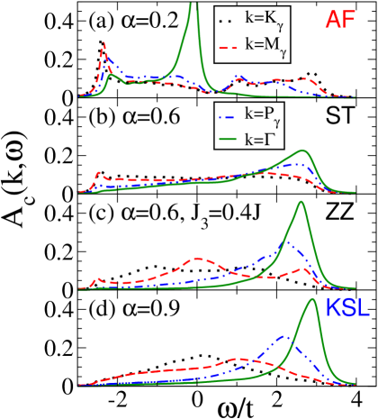
Figure 3: (Color online) Spectral function $A_{c}(\vec{k},\omega)$ (7) for one hole excitations notear at strong coupling, $t=5J$, obtained by ED at four distinct momenta $\vec{k}$ (solid, dashed, dashed-dotted and dotted lines) for: (a) the Néel phase at $\alpha=0.2$, (b,c) ST and ZZ phases at $\alpha=0.6$, and (d) the KSL phase at $\alpha=0.9$. Parameters: $J_{2}=0$, $\eta=0.1t$, and $J_{3}=0$, except in (c) where $J_{3}=0.4J$.

In all phases the spectra $A_{c}(\vec{k},\omega)$ and $A_{d}(\vec{k},\omega)$ shown in Figs. 3 and 4, respectively, have the total width $W\simeq 6t$ as for free hole motion on the honeycomb lattice. For small $\alpha<0.4$ the model (1) is weakly frustrated and $|0\rangle$ is the quantum AF Néel state, see Fig. 2(b). Taking $t/J=5$, a value representative for strong coupling ($t>J$) noteir , i.e., when the kinetic energy of a hole is larger than the energy of a magnetic bond, one finds that the spectral function $A_{c}(\vec{k},\omega)$ has a QP at low energy and its spectral weight is large at the $K_{\gamma}$ and much weaker at the $\Gamma$ point, see Fig. 3(a). In this phase no qualitative differences between $A_{c}(\vec{k},\omega)$ and $A_{d}(\vec{k},\omega)$ functions are observed, see Figs. 3(a) and 4(a), except near $\omega=0$ for the $\Gamma$ point.

The sublattice spectral function, $A_{d}(\vec{k},\omega)$, where holes are injected/removed on the same sublattice, reveals large spectral weight at low energy. For the ST and ZZ phases the low energy features in $A_{d}(\vec{k},\omega)$ can indeed be identified as QPs accompanied by incoherent spectral weight — they are more pronounced in the ZZ phase, cf. Figs. 4(b) and 4(c). Yet, the QP features are suppressed at the $\Gamma$ and $P$ points in these phases in the physical spectral function $A_{c}(\vec{k},\omega)$, cf. Figs. 3(b) and 3(c). As shown before Tro13 , this is consistent with the observed absence of QPs in ARPES for Na₂IrO₃ Com12 .

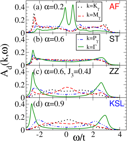
Figure 4: (Color online) Spectral function $A_{d}(\vec{k},\omega)$ (8) for a hole excitation created on one sublattice notear . The method, lines and parameters are the same as in Fig. 3.

The momentum $\vec{k}$ dependence of the low energy QPs shown in Fig. 5 reveals the strong dependence of hole dispersion on the magnetic order. As in cuprates Mar91 , the QP dispersion in the Néel AF phase is narrowed from the free (unconstrained) fermionic band width $\propto 6t$ by strong correlations and is determined by the magnetic exchange $\propto J_{1}$. The dispersion has a minimum (maximum) at the $K$ ($\Gamma$) point and is further reduced when frustration of magnetic exchange increases from $\alpha=0$ to $\alpha=0.2$ [Fig. 5(a)]. At finite $J_{3}$ the hole energy decreases at the $P$ point, but otherwise the dispersions at $\alpha=0.2$ are quite similar, cf. Figs. 5(a) and 5(b).

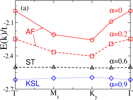
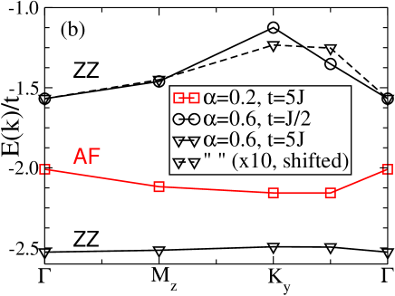
Figure 5: (Color online) Dispersion of lowest single hole energy obtained for the KH model Eq. (1) by ED for $t/J=5$, $J_{2}=0$, and increasing $\alpha$: (a) $J_{3}=0$, and (b) $J_{3}=0.5J$. Hole energies are respective to the ground state energy $E_{0}(N)$.

In contrast, the dispersion is absent in the ST phase, see Fig. 5(a), as coherent hole propagation is hindered here due to the alternating AF and FM bonds. Instead, for FM chains in the ZZ phase the dispersion appears reversed with respect to that found for the Néel phase — now a minimum (maximum) is at the $\Gamma$ ($K$) point. While this dispersion decreases from weak ($t=J/2$) to strong ($t=5J$) coupling, its shape remains the same [dashed line in Fig. 5(b)].

At first glance one might conclude from the spectral functions for the KSL, displayed in Figs. 3(d) and 4(d), that hole propagation in the KSL is similar to that in the ZZ phase [Figs. 5(a) and 5(b)]. In this case the lowest excitation energy is found at the $\Gamma$ point. Again, one finds a distinct peak in $A_{d}(\Gamma,\omega)$ which is absent in $A_{c}(\Gamma,\omega)$, suggesting also here a hidden QP. As shall see below that the fine structure of the low energy peaks in the spectral function shown in Fig. 4(d) does not represent well defined QPs in the case of the KSL.

IV Carrier propagation in the Kitaev spin-liquid phase

IV.1 Spectral weight distribution

Next we show that the KSL phase is manifestly different from all the ordered phases discussed so far. We address the nature of low energy states by analyzing first the intermediate coupling regime of $t/J=0.25$. Again one finds distinct low energy peaks in $A_{d}(\Gamma,\omega)$ note1 , see Fig. 6(b), missing in $A_{c}({\vec{k}},\omega)$ [Fig. 6(a)]. In contrast, both spectral functions are rigorously identical at the $K$ point, cf. $A_{c}(K,\omega)$ and $A_{d}(K,\omega)$ in Figs. 6(a) and 6(b). We note that for the honeycomb lattice $K$ corresponds to the Dirac point which is the degeneracy point of noninteracting electrons Gra09 .

A surprise comes when the fine structure of the sublattice spectral function is analyzed in absence of spectral broadening [at $\eta=0$ in Eq. (8)],

$$A_{d}^{(0)}(\vec{k},\omega)=\lim_{\eta\rightarrow 0}A_{d}(\vec{k},\omega),$$ (9)

which may be rewritten using spectral weights:

$$A_{d}^{(0)}(\vec{k},\omega)=\sum_{n}\alpha_{d}({\vec{k}},\omega_{n})\delta(\omega-\omega_{n})\,.$$ (10)

In the following we shall see the advantage of studying the single-particle propagation directly in terms of the spectral weight distribution,

$$\alpha_{d}({\vec{k}},\omega_{n})=|\langle\psi_{\vec{k},n}{(N-1)}|d_{\vec{k},\uparrow}|0\rangle|^{2},$$ (11)

at excitation energies

$$\omega_{n}=E_{\vec{k},n}{(N-1)}-E_{0}(N),$$ (12)

and $|\psi_{\vec{k},n}(N-1)\rangle$ is an excited state in the space with one extra hole and total momentum $\vec{k}$ that contributes with a finite spectral weight. We stress, that $\alpha_{d}({\vec{k}},\omega_{n})$ is in mathematical terms a distribution and not a function, although in the TL it may contain parts that can be represented by continuous curves, in some cases.

When looking at the spectral weight distribution in Fig. 6(c) we recognize a robust QP, that is, a well separated bound state at lowest energy, only at the $\Gamma$ point with large spectral weight $\alpha_{d}(\Gamma,\omega_{0})\simeq 0.45$. At all other ${\vec{k}}$ points no bound states exist but instead rather continuous distributions of weights $\alpha_{d}({\vec{k}},\omega_{n})$ is found in the range of the lowest eigenvalues $\omega_{n}$ (11). From the spectral weight distribution displayed in Fig. 6(c) it is clear that for example at the $P$ point the spectra are represented by a superposition of several many-body states in the $(N-1)$-particle sector with slightly different energies and there is no dominant pole that could be considered as a QP state. On the other hand, simply by looking at the spectral function $A_{d}(\vec{k},\omega)$ in Fig. 6(b) one may easily overlook the breakdown of the QP picture. We stress that in all cases there is substantial incoherent spectral weight at higher energies that extends to the upper edge of the spectrum at $6t$.

To understand this striking difference of the character of the spectra at low energy at $\Gamma$ and $P,M,K$, respectively, we need to investigate the spin excitations in the Kitaev liquid regime. Finally it is the scattering of carriers from spin excitations that determines whether they can propagate as QPs or whether they are completely overdamped.

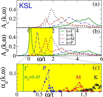
Figure 6: (Color online) Spectral functions for the KSL phase obtained by ED in the intermediate coupling regime $t/J=0.25$ at four nonequivalent momenta ${\vec{k}}$ (solid, dashed, dashed-dotted and dotted lines) with $\eta=0.1t$: (a) full spectral function $A_{c}(\vec{k},\omega)$, and (b) sublattice function $A_{d}(\vec{k},\omega)$. Panel (c) shows the spectral weights $\alpha_{d}({\vec{k}},\omega)$ (11) (symbols) larger than $3\times 10^{-3}$ at low energy (shaded) for different ${\vec{k}}$ values; dashed lines are guides to the eye. Parameters: $\alpha=0.9$, $J_{2}=J_{3}=0$.

IV.2 Spin excitations in Kitaev spin liquid

Our aim here is to explore the spin excitations of the KH model in the KSL regime. However, our discussion will be more transparent when we first focus on the pure Kitaev model at $\alpha=1$ and subsequently analyze by numerical simulation the changes of the spin structure factor for the KH case in the KSL regime ($0.8<\alpha<1.0$).

We shall employ here the usual representation of the Kitaev model in terms of $\sigma^{\gamma}_{i}=2S^{\gamma}_{i}$ spin operators

$$H_{K}=-\frac{1}{2}J\sum_{\langle ij\rangle\parallel\gamma}\sigma_{i}^{\gamma}\sigma_{j}^{\gamma},$$ (13)

where $J_{K}=-2J\alpha$ and $\alpha=1$, according to Eq. (1). Spin excitations are most easily understood by transforming the Kitaev model into the Majorana representation Kit06 . Kitaev introduced a representation for the spin algebra $[\sigma_{i}^{a},\sigma_{j}^{b}]=i\epsilon_{abc}\sigma_{i}^{c}\delta_{ij}$ in terms of four Majorana operators $\eta_{i}^{\gamma}$, $\gamma=0,x,y,z$, per lattice site which obey the anticommutation relations, $\{\eta^{\gamma},\eta^{\gamma^{\prime}}\}=2\delta_{\gamma,\gamma^{\prime}}$.

Here each spin operator component is expressed by a product of two Majorana fermions,

$$\sigma_{i}^{\alpha}=i\eta_{i}^{0}\eta_{i}^{\alpha},\hskip 14.22636pt\alpha=x,y,z,$$ (14)

where $\eta_{i}^{\alpha}$ is associated with the bond direction and $\eta_{i}^{0}=\eta_{i}$, with the respective vertex (at site $i$). We suppress the upper index in $\eta_{i}^{0}$ further on. Using this representation one can write the Hamiltonian as follows,

$$H_{K}=-\frac{1}{2}J\sum_{\langle ij\rangle_{\gamma}}i\eta_{i}u_{\langle ij\rangle}^{\gamma}\eta_{j},$$ (15)

where $u_{\langle ij\rangle}^{\alpha}$ are the bond operators,

$$u_{\langle ij\rangle}^{\alpha}=i\eta_{i}^{a}\eta_{j}^{\alpha}.$$ (16)

To take care of the fermionic property $u_{\langle ij\rangle}^{\alpha}=-u_{\langle ji\rangle}^{\alpha}$ we adopt a notation where $i(j)$ is on the $A(B)$ sublattice, respectively. The important point is now, that the so-defined bond operators (16) commute with the Hamiltonian,

$$[H_{K},u_{\langle ij\rangle}^{\alpha}]=0.$$ (17)

Hence they are conserved quantities and due to their definition as products of two Majoranas, see Eq. (16), these operators can only take the values $u_{\langle ij\rangle}^{\alpha}=\pm 1$.

In the ground state sector all $u_{\langle ij\rangle}^{\alpha}$ have the same sign on all bonds, either $+1$ or $-1$. A change of a bond variable leads to a vortex pair excitation with a gap $\Delta_{P}\simeq 0.26|J_{K}|$. In addition there is a second class of spin excitations which result from the motion of the $\eta$ Majorana particles described by the Hamiltonian in Eq. (15). Here we concentrate on the symmetric case, with equal exchange constants along three directions in the honeycomb lattice, $J_{x}=J_{y}=J_{z}$; in this case the Majorana excitations are gapless Kit06 .

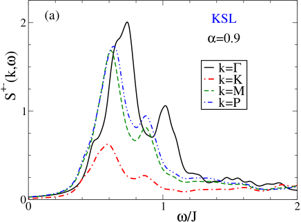
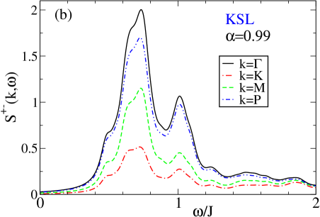
Figure 7: (Color online) Dynamic spin-structure factor $S^{+-}({\vec{k}},\omega)$ (18) for the undoped KSL in the case of the Kitaev-Heisenberg model Eq. (1) at four distinct momenta, for: (a) $\alpha=0.9$, and (b) $\alpha=0.99$. The curves are obtained by exact diagonalization of a 24-site cluster with periodic boundary conditions and are smoothened using a Lorentzian broadening $\eta=0.05J$.

Next we shall investigate the dynamic spin-structure factor in the Kitaev limit $\alpha\rightarrow 1$ by exact diagonalization and explore the changes in the Kitaev-liquid regime of the KH model for $\alpha\neq 1$, which cannot be solved analytically. This is demonstrated by a calculation of the dynamic spin-structure factor $S^{+-}({\vec{k}},\omega)$ defined as follows Toh95 ,

$$S^{+-}({\vec{k}},\omega)=\frac{1}{N}\sum_{\nu}|\langle{\nu}|S^{+}_{\vec{k}}|0\rangle|^{2}\delta(\omega-E_{\nu}+E_{0}),$$ (18)

where $S^{\gamma}_{\vec{k}}=\sum_{\vec{r}}e^{i{\vec{k}}\cdot{\vec{r}}}S_{\vec{r}}^{\gamma}$, and $\gamma=+,-$ denotes spin raising (lowering) operators, respectively. Here $|0\rangle$ and $|\nu\rangle$ are the ground and excited state, with energies $E_{0}$ and $E_{\nu}$, respectively. The spin quantization axis is chosen parallel to the $z$-th spin axis of the Kitaev term for convenience.

Figure 7(a) shows $S({\vec{k}},\omega)$ for the KH model Eq. (1) in the KSL regime at $\alpha=0.9$ for four different $\vec{k}$ points: $\Gamma$, $K$, $M$ and $P$. The numerical calculations were performed for a 24-site cluster with periodic boundary conditions. The main weight of the spin structure factor is concentrated between the vortex type spin gap at $\Delta_{s}\sim 0.4J$ and $\omega\sim 1.2J$. We observe a moderate momentum dependence with the vortex spin gap at $\Gamma$, $\Delta_{s}\sim 0.46J$ slightly larger than at $K$, $M$, and $P$, where we find $\Delta_{s}\sim 0.40J$. Moreover, we can conclude that the dispersion of the gap and of the peak structures is due to the Heisenberg terms in the Hamiltonian and disappears when one approaches the Kitaev limit Kno13 , as seen in Fig. 7(b).

Thus we find here that the main contributions to the spin-response as measured by dynamical spin-structure factor (18) come from the gapped vortex excitations. Furthermore the classification of spin excitations obtained for the pure Kitaev model as well as the spin gap due to vortex excitations appears still relevant for the KSL phase of the KH model Eq. (1) at $\alpha=0.9$.

IV.3 Hole motion in the Kitaev spin liquid:
Intermediate coupling

Our central argument why QPs at finite momentum are destroyed at intermediate coupling, as shown in Fig. 6(c), will be outlined next. Our explanation rests on the fact that there are two distinct types of elementary spin excitations from which the holes can scatter in the KSL. These excitations can be classified according to the exact solution given by Kitaev Kit06 as: (i) gapped vortex spin excitations with minimal gap $\Delta_{s}$, and (ii) gapless Majorana excitations.

We consider as intermediate coupling regime the range $0.1J<t<J$, where the kinetic energy of holes is comparable with the magnetic energy on the bonds, and not much larger as in the strong coupling regime, $J\ll t$. An important aspect of the spectral functions at intermediate coupling, as in the case of Fig. 6(c) which was calculated for $J=4t$, is the large size of the spin gap, $\Delta\simeq 0.4J\simeq 1.6t$ in units of the $t$-scale. As the excitation energies $\omega_{n}$ of the low energy states of holes at $P$, $M$ and $K$ relative to the bottom of the band at the $\Gamma$ point $\omega_{0}(\Gamma)$, are much smaller than the vortex spin gap $\Delta\simeq 1.6t$ at $J=4t$, no decay via vortex excitations Kit06 can occur. Therefore, we conclude that the destruction of QPs is due to the scattering of gapless Majorana fermion excitations, and that Fig. 6(c) has to be seen as a fingerprint of fractionalization of electrons into holons and gapless Majorana fermions of the Kitaev model Kit06 . Because of the dominant role of scattering from gapless spin-excitations we expect that in larger clusters with a denser $\vec{k}$-mesh, hole pockets near the $\Gamma$ point are not protected against strong scattering, and in consequence the KSL does not turn into a Fermi liquid at low doping.

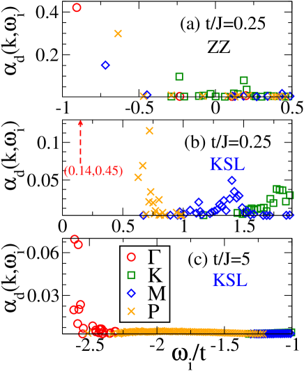
Figure 8: (Color online) Spectral weight distribution $\alpha_{d}(k,\omega)$, as obtained for: (a) the ZZ phase and (b) the KSL phase, both at intermediate coupling $t=0.25J$, and (c) the KSL phase at strong coupling $t=5J$. Parameters: (a) $\alpha=0.4$ and $J_{3}=0.5$; (b) and (c) $\alpha=0.9$ and $J_{3}=0$ in Eq. (1).

Before moving to the strong coupling regime $t\gg J$ we shall highlight the striking difference of the spectral weight distribution $\alpha_{d}(\vec{k},\omega_{n})$ (11) at low energy in the ZZ and the KSL phase, respectively, at $t=0.25J$. In Fig. 8(a) the spectral weight distribution $\alpha_{d}(\vec{k},\omega_{n})$ for the ZZ phase shows well defined QP bound states. Although the spectral weights of these QPs are significantly reduced, the bound states are well separated from the continuum (of incoherent states) at higher energy, except for $\vec{k}=K$ where this binding energy is much weaker. In the KSL phase Fig. 8(b), on the other hand, a well defined bound state is seen only at the $\Gamma$ point. Because of the size of the vortex gap $\Delta_{s}\simeq 1.6t$ the absence of QPs in Fig. 8(b) at $P$, $M$ and $K$ is a smoking gun for the important role played by scattering by gapless Majorana excitations. This is consistent with the spectral shape of $\alpha(\vec{k},\omega)$ which is reminiscent of a continuum, that may result from a convolution of holons and gapless Majorana fermions.

IV.4 Hole motion in the Kitaev spin liquid:
Strong coupling

We turn now to the strong coupling regime. In the strong coupling case of $t/J=5$, i.e., relevant for the iridates Com12 and displayed in Fig. 8(c), the vortex spin gap becomes small (in units of $t$), i.e., $\Delta_{s}=0.08$t. Thus the strong coupling result in Fig. 8(c) highlights the effect of the additional vortex excitations which form a new decay channel and damp the excitations at the $K$, $M$, and $P$ points even further. Compared to the result at intermediate coupling at $t=J/4$ [Fig. 8(b)] where the vortex gap is $\Delta_{s}=0.4J=1.6t$, at strong coupling one finds a spin gap to the vortex excitations which is 20 times smaller, that is $\Delta_{s}=0.08t$.

Furthermore, it may be instructive to go back to the spectral function $A_{d}(k,\omega)$ in Fig. 4(d) which basically contains the same information for the strong coupling case ($t=5J$) of the KSL as the spectral weight distribution shown in Fig. 8(c). The fine structure seen in $\alpha_{d}(\vec{k},\omega_{n})$ can only be resolved in $A_{d}(k,\omega)$ when the resolution parameter $\eta$ is taken small enough. For ARPES experiments, where actually $A_{c}(k,\omega)$ is measured, this implies that a sufficient momentum and energy resolution is required.

We conclude, that the peak at $\Gamma$, which appeared as a separate bound state at intermediate coupling in Fig. 8(b), appears now at strong coupling, see Fig. 8(c), rather as the edge of the continuum than as an isolated bound state. Moreover, when a single hole does not propagate as a QP, then a dilute gas of holes will not form a Fermi liquid. Therefore we stress, that the absence of a well defined separate bound state is a new qualitative feature which speaks against QPs and Fermi liquid behavior at low doping, and this time the argument emerges from a diagnosis at the $\Gamma$ point itself!

V Summary

We have shown that hole propagation is modified in a remarkable way as increasing Kitaev interactions drive the system from the Néel order via other ordered antiferromagnetic phases towards the Kitaev spin liquid. Quasiparticles are found in the Néel phase, whereas coherent hole propagation is hindered in stripe and zigzag phases, where hidden quasiparticles with weak dispersion result from coexisting ferromagnetic and antiferromagnetic bonds. As the most unexpected result, in the Kitaev liquid phase we have found unprecedented spectral weight distribution at low energy that signals the absence of quasiparticles, both at intermediate and strong coupling. Thus, it appears clearly that carrier motion in the lightly doped Kitaev liquid is non-Fermi liquid like.

The above conclusion follows from the short-range nature of spin correlations in the Kitaev spin liquid Bas07 . Unlike in a quantum antiferromagnet on a square Mar91 or honeycomb Sus06 lattice where spin-flip processes couple to a moving hole and generate new energy scale for coherent hole propagation, the Kitaev spin-liquid phase is characterized by Ising-like nearest neighbor spin correlations of one spin component. Such correlations are insufficient to generate coherent hole propagation. They are well captured by the present cluster size of $N=24$ sites, and qualitative changes of the described scenario are therefore unexpected when the cluster size is increased.

Summarizing, we have given clear arguments that shed serious doubts on the claim from a slave-boson approximation, namely that the low doped Kitaev spin-liquid phase is a Fermi liquid Mei12 . The first of these arguments rests on the exact solution for the spin excitations in the Kitaev model in the intermediate coupling regime, and on our finding that gapless Majorana excitations are responsible for the absence of QPs away from the $\Gamma$ point. From the gaplessness we conclude that also states in the closer vicinity of $\Gamma$ are not protected.

Our second argument emerges in the strong coupling case from the result for the spectral distribution $\alpha_{d}(\vec{k},\omega)$ at the $\Gamma$ point itself, which in this case has no similarity to a QP but appears rather as the edge of a continuum. We consider this as evidence that at strong coupling there are no QPs in the single hole case near the $\Gamma$ point, and from this finding we can safely conclude that Fermi liquid behavior is absent in the low doping regime.

- (1) Elbio Dagotto, Rev. Mod. Phys. 66, 763 (1994).
- (2) K. J. von Szczepanski, P. Horsch, W. Stephan, and M. Ziegler, Phys. Rev. B 41, 2017 (1990).
- (3) V. J. Emery, S. A. Kivelson, and O. Zachar, Phys. Rev. B 56, 6120 (1997).
- (4) P. A. Lee, N. Nagaosa, and X.-G. Wen, Rev. Mod. Phys. 78, 17 (2006); M. Ogata and H. Fukuyama, Rep. Prog. Phys. 71, 036501 (2008).
- (5) P. W. Anderson, Phys. Rev. Lett. 64, 1839 (1990); Z. Y. Weng, D. N. Sheng, Y.-C. Chen, and C. S. Ting, Phys. Rev. B 55, 3894 (1997).
- (6) W. F. Brinkman and T. M. Rice, Phys. Rev. B 2, 1324 (1970).
- (7) S. A. Trugman, Phys. Rev. B 37, 1597 (1988); C. D. Batista and G. Ortiz, Phys. Rev. Lett. 85, 4755 (2000); M. Daghofer, K. Wohlfeld, A. M. Oleś, E. Arrigoni, and P. Horsch, ibid. 100, 066403 (2008); K. Wohlfeld, M. Daghofer, A. M. Oleś, and P. Horsch, Phys. Rev. B 78, 214423 (2008); K. Wohlfeld, A. M. Oleś, and P. Horsch, ibid. 79, 224433 (2009); W. Brzezicki, M. Daghofer, and A. M. Oleś, ibid. 89, 024417 (2014); A. M. Oleś, J. Phys.: Condens. Matter 24, 313201 (2012).
- (8) C. L. Kane, P. A. Lee, and N. Read, Phys. Rev. B 39, 6880 (1989); G. Martinez and P. Horsch, ibid. 44, 317 (1991); A. Ramšak and P. Horsch, ibid. 57, 4308 (1998); Z. P. Liu and E. Manousakis, ibid. 44, 2414 (1991); 45, 2425 (1992); P. Wróbel and R. Eder, ibid. 58, 15160 (1998); J. Bonča, S. Maekawa, and T. Tohyama, ibid. 76, 035121 (2007); I. J. Hamad, A. E. Trumper, A. E. Feiguin, and L. O. Manuel, ibid. 77, 014410 (2008).
- (9) A. Damascelli, Z. Hussain, and Z.-X. Shen, Rev. Mod. Phys. 75, 473 (2003).
- (10) A. Lüscher, A. Läuchli, W. Zheng, and O. P. Sushkov, Phys. Rev. B 73, 155118 (2006).
- (11) R. Comin et al., Phys. Rev. Lett. 109, 266406 (2012).
- (12) F. Trousselet, M. Berciu, A. M. Oleś, and P. Horsch, Phys. Rev. Lett. 111, 037205 (2013).
- (13) H. Lei, W.-G. Yin, Z. Zhong, and H. Hosono, Phys. Rev. B 89, 020409(R) (2014).
- (14) A. H. Castro Neto, F. Guinea, N. M. R. Peres, K. S. Novoselov, and A. K. Geim, Rev. Mod. Phys. 81, 109 (2009).
- (15) M. Polini, F. Guinea, M. Lewenstein, H. C. Manoharan, and V. Pellegrini, Nature Nanotechnology 8, 625 (2013).
- (16) C. Wu, D. Bergman, L. Balents, and S. Das Sarma, Phys. Rev. Lett. 99, 070401 (2007); B. Wunsch, F. Guinea, and F. Sols, New J. Phys. 10, 103027 (2008).
- (17) M. Hohenadler and F. F. Assaad, J. Phys.: Condens. Matter 25, 143201 (2013).
- (18) Bruce Normand, Cont. Phys. 50, 533 (2009).
- (19) Leon Balents, Nature (London) 464, 199 (2010).
- (20) A. Y. Kitaev, Ann. Phys. (N.Y.) 321, 2 (2006).
- (21) Z. Nussinov and J. van den Brink, arXiv:1303.5922 (unpublished).
- (22) G. Jackeli and G. Khaliullin, Phys. Rev. Lett. 102, 017205 (2009).
- (23) Z. Y. Meng, T. C. Lang, S. Wessel, F. F. Assaad, and A. Muramatsu, Nature (London) 464, 847 (2010); S. Sorella, Y. Otsuka, and S. Yunoki, Sci. Rep. 2, 992 (2012).
- (24) J. Chaloupka, G. Jackeli, and G. Khaliullin, Phys. Rev. Lett. 105, 027204 (2010); 110, 097204 (2013).
- (25) H.-C. Jiang, Z.-C. Gu, X.-L. Qi, and S. Trebst, Phys. Rev. B 83, 245104 (2011); J. Reuther, R. Thomale, and S. Trebst, ibid. 84, 100406 (2011); R. Schaffer, S. Bhattacharjee, and Y. B. Kim, ibid. 86, 224417 (2012); I. Kimchi and Y. Z. You, ibid. 84, 180407 (2011); Y. Yu, L. Liang, Q. Niu, and S. Qin, ibid. 87, 041107 (2013).
- (26) A. Shitade, H. Katsura, J. Kuneš, X.-L. Qi, S.-C. Zhang, and N. Nagaosa, Phys. Rev. Lett. 102, 256403 (2009).
- (27) G. Baskaran, S. Mandal, and R. Shankar, Phys. Rev. Lett. 98, 247201 (2007); S. R. Hassan, P. V. Sriluckshmy, S. K. Goyal, R. Shankar, and D. Sénéchal, ibid. 110, 037201 (2013).
- (28) P. Horsch, G. Khaliullin, and A. M. Oleś, Phys. Rev. Lett. 91, 257203 (2003).
- (29) Y. Singh and P. Gegenwart, Phys. Rev. B 82, 064412 (2010); X. Liu, T. Berlijn, W.-G. Yin, W. Ku, A. Tsvelik, Y.-J. Kim, H. Gretarsson, Y. Singh, P. Gegenwart, and J. P. Hill, ibid. 83, 220403 (2011).
- (30) Y. Singh, S. Manni, J. Reuther, T. Berlijn, R. Thomale, W. Ku, S. Trebst, and P. Gegenwart, Phys. Rev. Lett. 108, 127203 (2012); S. K. Choi et al., ibid. 108, 127204 (2012).
- (31) F. Ye, S. Chi, H. Cao, B. C. Chakoumakos, J. A. Fernandez-Baca, R. Custelcean, T. F. Qi, O. B. Korneta, and G. Cao, Phys. Rev. B 85, 180403 (2012).
- (32) A. F. Albuquerque, D. Schwandt, B. Hetényi, S. Capponi, M. Mambrini, and A.M. Laüchli, Phys. Rev. B 84, 024406 (2011); D. C. Cabra, C. A. Lamas, and H. D. Rosales, ibid. 83, 094506 (2011); H. D. Rosales, D. C. Cabra, C. A. Lamas, P. Pujol, and M.E. Zhitomirsky, ibid. 87, 104402 (2013); A. Kalz, M. Arlego, D. Cabra, A. Honecker, and G. Rossini, ibid. 85, 104505 (2012).
- (33) R. Ganesh, J. van den Brink, and S. Nishimoto, Phys. Rev. Lett. 110, 127203 (2013); R. Ganesh, S. Nishimoto, and J. van den Brink, Phys. Rev. B 87, 054413 (2013); Z. Zhu, D.A. Huse, and S. R. White, Phys. Rev. Lett. 110, 127205 (2013).
- (34) J. G. Rau, E. K.-H. Lee, and H.-Y. Kee, Phys. Rev. Lett. 112, 077204 (2014).
- (35) T. Senthil, S. Sachdev, and M. Vojta, Phys. Rev. Lett. 90, 216403 (2003).
- (36) T. Hyart, A. R. Wright, G. Khaliullin, and B. Rosenow, Phys. Rev. B 85, 140510 (2012).
- (37) Y.-Z. You, I. Kimchi, and A. Vishwanath, ibid. 86, 085145 (2012).
- (38) S. Okamoto, Phys. Rev. Lett. 110, 066403 (2013); Phys. Rev. B 87, 064508 (2013).
- (39) F. J. Burnell and C. Nayak, Phys. Rev. B 84, 125125 (2011).
- (40) Jin-Wei Mei, Phys. Rev. Lett. 108, 227207 (2012).
- (41) A. Läuchli and D. Poilblanc, Phys. Rev. Lett. 92, 236404 (2004).
- (42) T. A. Kaplan, P. Horsch, and W. von der Linden, J. Phys. Soc. Jpn. 58, 3894 (1989).
- (43) T. Koma and H. Tasaki, J. Stat. Phys.76, 745 (1994).
- (44) F. Trousselet, G. Khaliullin, and P. Horsch, Phys. Rev. B 84, 054409 (2011).
- (45) The relatively large value seen for is due to the smallness of the cluster and consistent with spin correlations calculated in Ref. Bas07 .
- (46) W.-L. You, Y.-W. Li, and S.-J. Gu, Phys. Rev. E 76, 022101 (2007).
- (47) Shi-Jian Gu, Int. J. Mod. Phys. B 24, 4371 (2010).
- (48) E. R. Gagliano and C. A. Balseiro, Phys. Rev. Lett. 59, 2999 (1987).
- (49) Strong coupling regime is expected for Na2IrO3 Tro13 .
- (50) Spectral function is similar at low for .
- (51) In our definition of Eq. (7), we plot increasing ARPES excitation energies from left to right.
- (52) T. Tohyama, P. Horsch, and S. Maekawa, Phys. Rev. Lett. 74, 980 (1995).
- (53) J. Knolle, D. L. Kovrizhin, J. T. Chalker, and R. Moessner, arXiv:1308.4336.