Guiding synchrony through random networks

Abstract

Sparse random networks contain structures that can be considered as diluted feed-forward networks. Modeling of cortical circuits has shown that feed-forward structures, if strongly pronounced compared to the embedding random network, enable reliable signal transmission by propagating localized (sub-network) synchrony. This assumed prominence, however, is not experimentally observed in local cortical circuits. Here we show that nonlinear dendritic interactions as discovered in recent single neuron experiments, naturally enable guided synchrony propagation already in random recurrent neural networks exhibiting mildly enhanced, biologically plausible sub-structures.

I Introduction

Cortical neural networks generate a ground state of highly irregular spiking activity whose dynamics is sensitive to small perturbations such as missing or additional spikes [1, 2, 3, 4]. A robust, reliable transmission of information in the presence of such perturbations and noise is nonetheless assumed to be essential for neural computation. It has been hypothesized that this might be achieved by propagation of pulses of synchronous spikes along feed-forward chains [5]. In current models, functionally relevant chains require a dense connectivity between the neuronal layers of the network [6] or strongly enhanced synapses and specifically modified response properties of neurons within the chain [7]. Such highly distinguished large-scale structures however are not observed experimentally.

Can less structured networks also guide synchrony? Recently, single neuron experiments have revealed a mechanism that nonlinearly promotes synchronous inputs. Upon synchronous dendritic stimulation, neurons are capable of generating fast dendritic spikes. In the soma, these induce rapid, strong depolarizations [8] that are nonlinearly enhanced compared to depolarizations expected from linear summation of single inputs. If the dendritic spike induces an action potential in the soma, the latter occurs at a fixed time after the stimulation, with sub-millisecond precision. Other experiments have found slow dendritic spikes which are comparably insensitive to input synchrony [9]. These slow dendritic spikes endow single neurons with computational capabilities comparable to multi-layered feed-forward networks of simple rate neurons [10]. Furthermore, they provide a possible mechanism underlying neural bursting and its propagation, which have been shown to enhance reliability and temporal precision of signal propagation [11, 12]. The impact of fast dendritic spikes that induce non-additive coupling, on collective circuit dynamics has not been systematically investigated so far in a general setting.

In this article, we show that and how fast dendritic nonlinearities may support guided synchrony propagation in neural circuits. First, we develop an analytical approach to describe such propagation in linearly and nonlinearly coupled networks. In particular, we derive an expression for the critical connectivity above which propagation occurs and for the size of the propagating pulse. We quantify how dendritic nonlinearities compensate for dense anatomical connections and thereby promote propagation of synchrony. Finally, using large-scale simulations of more detailed recurrent network models, we show that feed-forward networks that occur naturally as part of random circuits enable persistent guided synchrony propagation due to dendritic nonlinearities.

II Models and Methods

II.1 Analytically tractable model

Model with linear summation of inputs. As a basis model we consider networks of conventional leaky integrate-and-fire neurons that interact by sending and receiving spikes via directed connections. The membrane potential $V_{l}$ of a neuron $l$ satisfies

$$\dot{V}_{l}(t)=-\gamma_{l}V_{l}(t)+I_{l}\left(t\right),$$ (1)

where $\gamma_{l}$ is the inverse membrane time constant and $I_{l}(t)$ is the total input current at time $t$. In addition to inputs from the network, the neurons receive excitatory and inhibitory random inputs which emulate an embedding network, i.e.

$$I_{l}(t)=I_{l}^{0}+I_{l}^{\text{ext,ex}}(t)+I_{l}^{\text{ext,in}}(t)+I_{l}^{\text{net}}(t),$$ (2)

where $I_{l}^{0}$ is a constant input current modeling slow external (from outside the chain) and internal (from the chain) currents, $I_{l}^{\text{ext,ex}}(t)$ and $I_{l}^{\text{ext,in}}(t)$ are the contributions due to arriving external excitatory and inhibitory spikes (that are modeled as independent random (Poissonian) spike trains with rate $\nu^{\text{ext,ex}}$ and $\nu^{\text{ext,in}}$ respectively) and $I_{l}^{\text{net}}(t)$ are the contributions originating from spikes of neurons of the network. In the absence of any spiking activity, the membrane potential will exponentially converge towards its asymptotic value $V_{l}^{\infty}:=I_{l}^{0}/\gamma_{l}$. When the neuron’s membrane potential reaches or exceeds its threshold $\Theta_{l}$, its membrane potential is reset to $V_{l}^{\text{reset}}$ and a spike is emitted, which arrives at the postsynaptic neuron $j$ after a delay time $\tau_{jl}$. For a refractory period $t_{l}^{\text{ref}}$ after the reset, all incoming spikes to neuron $l$ are ignored and the membrane potential is kept at $V_{l}^{\text{reset}}$.

We model the fast rise of the membrane potential upon the arrival of a presynaptic spike by an instantaneous jump, such that the contributions of the arriving external spikes to the total input current are given by

$$I_{l}^{\text{ext,ex}}(t) = \sum_{k\in\mathbb{Z}}\epsilon^{\text{ext,ex}}\cdot\delta\left(t-t_{l,k}^{\text{ext,ex}}\right),$$ (3)

$$I_{l}^{\text{ext,in}}(t) = \sum_{k\in\mathbb{Z}}\epsilon^{\text{ext,in}}\cdot\delta\left(t-t_{l,k}^{\text{ext,in}}\right),$$ (4)

where $t_{l,k}^{\text{ext,ex}}$ ($t_{l,k}^{\text{ext,in}}$) are the arrival times of the $k$th excitatory (inhibitory) external spike at neuron $l$, $\epsilon^{\text{ext,ex}}>0$ or $\epsilon^{\text{ext,in}}<0$ are the strengths of single external spikes and $\delta(\cdot)$ is the Dirac $\delta$-distribution. Analogously the contribution of spikes received from neurons of the network is given by

$$I_{l}^{\text{net}}\left(t\right)=\sum_{j}\sum_{k}\epsilon_{lj}\delta\left(t-t_{j,k}^{f}-\tau_{lj}\right),$$ (5)

where $\epsilon_{lj}$ is the coupling strength from neuron $j$ to $l$ and $t_{j,k}^{f}$ is the $k$th spike time of neuron $j$.

Model with nonlinear summation of inputs. In the above model without nonlinear dendrites, the strengths of synchronous inputs are summed up linearly (cf. Eq. (5)). We incorporate nonlinear dendrites by modulating this sum for excitatory inputs by a nonlinear function $\sigma$, that can be directly read off from experimental results [8]: $\sigma$ equals the identity for small excitatory input, increases steeply when the input exceeds a threshold $\Theta_{b}$ and saturates for larger inputs. We define the dendritic modulation function as

$$\sigma\left(\epsilon\right)=\begin{cases}\epsilon&\text{for }\epsilon\leq\Theta_{b}\\ \kappa&\text{otherwise}\end{cases}.$$ (6)

For simplicity, we consider only exactly simultaneous spikes as synchronous. Accordingly, conduction delays are chosen homogeneously, $\tau_{ij}\equiv\tau$, so that synchronous presynaptic spiking can be amplified. In this scenario the detection of synchronous events is straightforward. However, systems with heterogeneous delays and finite dendritic integration window exhibit qualitatively the same phenomena [13]. The contribution of spikes received from the network is then given by

$$I_{l}^{\text{net}}(t) = \sum_{t^{f}}\left[\sigma\left(\sum_{j\in M_{ex}\left(t^{f}\right)}\epsilon_{lj}\right)+\sum_{j\in M_{in}\left(t^{f}\right)}\epsilon_{lj}\right]$$ (7)

$$\quad\times\delta\left(t-t^{f}-\tau\right),$$

where $t^{f}$ are all firing times in the network. The sets $M_{ex}(t^{f})$ and $M_{in}(t^{f})$ denote the sets of indices of neurons sending an excitatory and inhibitory spike at time $t^{f}$, respectively. Networks with linear dendrites can be described by setting $\sigma(\epsilon)=\epsilon$.

II.2 Biologically more detailed model

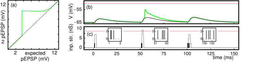
Figure 1: (color) Example dynamics of a conductance-based leaky integrate-and-fire neuron with dendritic spike generation (the neuron is initially at resting membrane potential $V^{\text{rest}}=-65$mV, there are no external inputs and $I^{0}=0$). Panel (a) shows the pEPSP after a stimulation versus the expected pEPSP, i.e. the pEPSP for a neuron without dendritic spike generation. For inputs corresponding to a pEPSP larger than $\approx 3.8$mV, a dendritic spike is generated which leads to a higher depolarization than expected from additive integration. Panel (b) shows the time course of the membrane potential of a neuron with (green) and without (black) nonlinear dendritic interaction in response to different excitatory inputs sequences (red horizontal line: somatic spike threshold). Panel (c) shows the input sequences (black lines, strength: $g^{\text{ex}}=2.3$nS, closeups given by insets) and the sum $g_{l,\Delta t}(t)$ of excitatory inputs received within the dendritic integration window $[t-\Delta t,t]$ (gray), cf. Eq. (9). At the first spike arrival around $t=1$ms, three inputs are received within $\Delta t$ such that $g_{l,\Delta t}(t)$ reaches $6.9$nS. The sum is smaller than the dendritic threshold $g^{\Theta}=8.65$nS (red horizontal line in c), so no dendritic spike is generated and there is no difference between the membrane potential for a neuron with and without a mechanism for dendritic spike generation. Around $t=50$ms, four spikes arrive within $\Delta t$, $g_{l,\Delta t}(t)$ exceeds the dendritic threshold and a dendritic spike is generated. Around $t=100$ms four spikes arrive at the neuron, but the temporal difference between the last and the first spike is slightly larger than $\Delta t$. Consequently, $g_{l,\Delta t}(t)$ does not exceed the dendritic threshold and no dendritic spike is initiated.

Conductance based model. In the last part of the article we employ a biologically more detailed neuron model to highlight the generality of our findings on propagation enhancement. The neuron model is a conductance-based leaky integrate-and-fire neuron that is augmented by terms introducing the impact of dendritic spikes (see also [14]). The subthreshold dynamics of the membrane potential $V_{l}$ of neuron $l$ obeys the differential equation

$$C_{l}^{\text{m}}\frac{dV_{l}(t)}{dt}=g_{l}^{L}\left(V_{l}^{\text{rest}}-V_{l}(t)\right)+g_{l}^{A}(t)\left(E^{\text{Ex}}-V_{l}(t)\right)+g_{l}^{G}(t)\left(E^{\text{In}}-V_{l}(t)\right)+I_{l}^{\text{DS}}(t)+I_{l}^{0}.$$ (8)

Here, $C_{l}^{\text{m}}$ is the membrane capacity, $g_{l}^{L}$ is the resting conductance and $V_{l}^{\text{rest}}$ is the resting membrane potential, $E^{\text{Ex}}$ and $E^{\text{In}}$ are the reversal potentials, and $g_{l}^{A}(t)$ and $g_{l}^{G}(t)$ are the conductances of excitatory and inhibitory synaptic populations, respectively. $I_{l}^{\text{DS}}(t)$ models the current pulses caused by dendritic spikes and $I_{l}^{0}$ is a constant current gathering slow external and internal currents. The time course of single synaptic conductances contributing to $g_{l}^{A}(t)$ and $g_{l}^{G}(t)$ is given by the difference between two exponential functions (e.g. [15]). Whenever the membrane potential reaches the spike threshold $\Theta_{l}$, the neuron sends a spike to its postsynaptic neurons, is reset to $V_{l}^{\text{reset}}$ and becomes refractory for a period $t_{l}^{\text{ref}}$.

To account for dendritic spike generation, we consider the sum $g_{l,\Delta t}$ of excitatory input strengths (characterized by the coupling strengths) arriving at an excitatory neuron $l$ within the time window $\Delta t$ for nonlinear dendritic interactions,

$$g_{l,\Delta t}(t)=\sum_{j}\sum_{k}g_{lj}^{\text{max}}\chi_{\left[t,t-\Delta t\right]}(t_{j,k}^{f}+\tau),$$ (9)

where $\chi_{\left[t,t-\Delta t\right]}$ is the characteristic function of the interval $[t,t-\Delta t]$, $t_{j,k}^{f}$ is the $k$th firing time of excitatory neuron $j$ and $\tau$ denotes the synaptic delay. We denote the peak conductance (coupling strength) for a connection from neuron $j$ to neuron $l$ by $g_{lj}^{\text{max}}$. If $g_{l,\Delta t}$ exceeds a threshold $g_{\Theta}$, a dendritic spike is initiated and the dendrite becomes refractory for a time window $t^{\text{DS,ref}}$. The effect of the dendritic spike is incorporated into the model by the current pulse that reaches the soma a time $\tau^{\text{DS}}$ thereafter. This current pulse is modeled as the sum of three exponential functions,

$$I_{l}^{\text{DS}}(t)=c(g_{\Delta t})\left[-Ae^{-\frac{t}{\tau^{\text{DS,1}}}}+Be^{-\frac{t}{\tau^{\text{DS,2}}}}-Ce^{-\frac{t}{\tau^{\text{DS,3}}}}\right],$$ (10)

with prefactors $A>0$, $B>0$, $C>0$, decay time constants $\tau^{\text{DS,1}}$, $\tau^{\text{DS,2}}$, $\tau^{\text{DS,3}}$ and a dimensionless correction factor $c\left(g_{\Delta t}\right)$, where $g_{\Delta t}$ is the summed excitatory input at the initiation time of the dendritic spike as given by Eq. (9). The factor $c\left(g_{\Delta t}\right)$ modulates the pulse strength, ensuring that the peak of the excitatory postsynaptic potential (pEPSP) reaches the experimentally observed region of saturation. At very high excitatory inputs, the conventionally generated depolarization exceeds the level of saturation, and the pEPSP increases (cf. Fig. (1)a).

Detection probability. In the last part of the article we investigate recurrent networks, where a feed-forward subnetwork consisting of a certain number of layers (groups) is created by modifying strengths of existing synaptic connections of the network. To decide whether propagation of synchrony in recurrent networks is successful, we consider the signal to noise ratio (SNR): We pick $\omega$ neurons, randomly selected from the network, to be a first group. After initiation of synchronous activity in this group, we count the number of spikes from neurons of the $i^{\text{th}}$ group (for details on how the $i^{\text{th}}$ group is defined, see section on recurrent networks), $S_{i}$, within a time window $\left[t_{i}^{\text{exp}}-\frac{t^{w}}{2},t_{i}^{\text{exp}}+\frac{t^{w}}{2}\right]$. Here $t_{i}^{\text{exp}}$ is the expected time for the synchronous pulse to reach layer $i$ and $t^{w}$ is the expected width of the synchronous pulse. We consider all spikes within the time window of size $t^{w}$ centered at $t_{i}^{\text{exp}}$ as part of the synchronous pulse. We assume that $t_{i}^{\text{exp}}=t_{1}^{\exp}+\left(i-1\right)\Delta t^{\text{exp}}$, where $\Delta t^{\text{exp}}$ itself is chosen after simulation such that $\sum_{i}S_{i}$ becomes maximal,

$$S_{i}=\sum_{k}\sum_{j\in\text{Gr}\left(i\right)}\chi_{\left[t_{i}^{\text{exp}}-\frac{t^{w}}{2},t_{i}^{\exp}+\frac{t^{w}}{2}\right]}\left(t_{j,k}^{f}\right).$$ (11)

Here, $\text{Gr}\left(i\right)$ are the indices of neurons of group $i$, $t_{j,k}^{f}$ is the $k^{\text{th }}$ firing time of neuron $j$ and $\chi$ denotes the characteristic function, as before.

To determine the noise level of group $i$, we measure the probability $P_{\Delta t^{\text{obs}},t^{w}}^{i}(k)$ of finding $k$ spikes from neurons of group $i$ within time windows $t^{w}$ over a control time interval where no synchronous activity is initiated. The noise level $N_{i}$ of group $i$ is the minimal value satisfying

$$\sum_{k=0}^{N_{i}}P_{\Delta t^{\text{obs}},t^{w}}^{i}\left(k\right)\geq a,$$ (12)

with a constant $a\lesssim 1.$

Finally, we denote the propagation of synchrony up to the $i^{\text{th}}$ layer as successful, if the SNR is larger than b,

$$\text{SNR}_{i}:=\min_{j=1,\dots,i}\left\{\frac{S_{j}}{N_{j}}\right\}>b,$$ (13)

where $b\geq 1.$ This means in particular that we can distinguish the background (spontaneous) activity from the signal induced by propagation of synchrony in all layers $1,\ldots,i$.

III Results

III.1 Feed-forward chains with linear coupling

How can diluted feed-forward networks (FFNs) propagate synchrony? FFNs consist of a sequence of layers, each composed of $\omega$ excitatory neurons, and forward connections to neurons in the subsequent layer randomly present with probability $p$. Present connections have strength $\epsilon$. Synchronous spiking activity is initiated by exciting neurons of the first layer to spike simultaneously. In the second layer they excite a certain subgroup of neurons to spike simultaneously that in turn generates a synchronous input to layer three, etc.

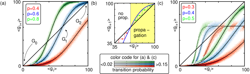
Figure 2: (color online) Emergence of propagation of synchrony. (a) Analytically derived iterated maps approximating the time evolution of the synchronous pulse (solid line, cf. Eq. (16)) and transition probability obtained from network simulations (color code). (b) The basin of attraction of the stable fixed point $G_{2}$ is illustrated: Initial pulses within the range $\left(G_{1},\omega\right]$ will propagate with an average pulse size around $G_{2}$. (c) Iterated maps for FFNs with linear (solid) and nonlinear dendritic interactions (dashed). Nonlinear interactions reduce the connectivity required for propagation and allow for smaller fractions of active neurons.

To understand the collective dynamics analytically, we consider networks of leaky integrate-and-fire neurons in the limit of fast synaptic currents (cf. Section “Models and Methods”). In the absence of synchronous activity, each neuron of the FFN receives a large number of inputs from an emulated external network and only very few inputs from the previous layer, such that its dynamics is practically identical to the ground state of balanced networks. If the connections within the FFN are weak and/or the connection probability is low, the spontaneous spiking activity is only weakly influenced by spiking activity of the FFN. Therefore, we assume that the ground state activity is exclusively governed by the external inputs, effectively setting couplings within the chain to $\epsilon_{ij}=0$. The external input is balanced, i.e. the mean input is subthreshold and spontaneous spiking is caused by fluctuations in the input. The network’s neurons thus spike in an asynchronous and irregular manner [2, 1] and the stationary distribution of membrane potentials $P_{V}(V)$ can be calculated analytically in diffusion approximation [2, 16].

$$p_{f}(x):=\int_{\Theta-x}^{\Theta}P_{V}(V)dV$$ (14)

is the probability of finding a neuron’s membrane potential in the interval $\left[\Theta-x,\Theta\right]$. We model the fast rise of the membrane potential upon the arrival of (possibly nonlinear enhanced) presynaptic spikes by an instantaneous jump in the membrane potential (cf. Section “Models and Methods”), thus $p_{f}\left(\sigma\left(h\epsilon\right)\right)$ specifies the spiking probability of a single neuron, after receiving $h$ input spikes of strength $\epsilon$ from the preceding layer.

To assess the propagation of synchrony, we consider the average number of neurons which are activated in each layer in response to the initial synchronous pulse (cf. also [17]). When $g_{i}$ neurons spike synchronously in layer $i$,

$$p^{\text{sp}}(g_{i}):=\sum_{h=0}^{g_{i}}\binom{g_{i}}{h}p^{h}\left(1-p\right){}^{g_{i}-h}p_{f}\left(\sigma\left(h\epsilon\right)\right)$$ (15)

is the probability of spiking of a particular neuron in layer $i+1$, where the number of simultaneous inputs $h$ is binomially distributed, $h\sim B(g_{i},p)$. Thus, for layers of size $\omega$, the average number of neurons spiking in layer $i+1$ is

$$\left\langle g_{i+1}\right\rangle=\omega p^{\text{sp}}\left(g_{i}\right).$$ (16)

Substituting the average group size $\left\langle g_{i}\right\rangle$ for the actual size $g_{i}$ yields the interpolated map $\left\langle g_{i+1}\right\rangle=\omega p^{\text{sp}}\left(\left\langle g_{i}\right\rangle\right),$ whose fixed points qualitatively determine the propagation of synchronous activity, cf. Fig. 2.

The trivial, absorbing fixed point $G_{0}=0$, defining a state of extinguished activity always exists. For sufficiently small $p$, $\epsilon$ and $\omega$, this is the only fixed point. With increasing connectivity and layer size, a pair of fixed points ($G_{1}$, unstable, and $G_{2}$, stable) appears via a tangent bifurcation. Initial pulses in the basin of $G_{2}$ (i.e. those larger than $G_{1}$) typically initiate stable propagation of synchrony with group sizes around $G_{2}$. For given layer size $\omega$ and connection strength $\epsilon$, the critical connectivity $p^{\ast}$ for which $G_{1}=G_{2}$ marks the minimal connectivity that supports stable propagation of synchrony.

To elaborate the influence of nonlinear dendritic interactions, we derive the critical connectivity for FFNs. The mechanisms underlying propagation of synchrony are different for networks with and without nonlinear dendritic interactions and thus require different analytical approaches to derive $p^{\ast}$. We first consider feed-forward chains with conventional, linear coupling, i.e. $\sigma(x)=x$. To obtain $p^{\ast}$, we first expand $p_{f}(x)$ into a Taylor series up to first order around the mean of the binomial distribution specifying the average number $pg_{i}$ of active neurons in each layer, such that Eq. (16) simplifies to

$$\left\langle g_{i+1}\right\rangle = \omega\sum_{h=0}^{g_{i}}\binom{g_{i}}{h}p^{h}\left(1-p\right){}^{g_{i}-h}p_{f}\left(h\epsilon\right)$$ (17)

$$\stackrel{{\scriptstyle\cdot}}{{=}} \omega\sum_{h=0}^{g_{i}}\binom{g_{i}}{h}p^{h}\left(1-p\right){}^{g_{i}-h}$$ (19)

$$\quad\times\left(p_{f}\left(g_{i}p\epsilon\right)+p_{f}^{\prime}(g_{i}p\epsilon)(h\epsilon-g_{i}p\epsilon)\right)$$

$$= \omega p_{f}(g_{i}p\epsilon).$$ (20)

The linear approximation becomes exact in the limit of large layer sizes $\omega$ and small couplings $\epsilon$, where the product $\epsilon\omega$ is kept constant. We obtain an interpolated map from Eq. (20) by replacing $g_{i}$ by its mean value $\left\langle g_{i}\right\rangle$. At the fixed point $G:=\left\langle g_{i+1}\right\rangle=\left\langle g_{i}\right\rangle$, the function

$$F(G,p^{\dagger},\omega,\epsilon):=G-\omega p_{f}(p^{\dagger}G\epsilon)=0$$ (21)

vanishes. Here, the values $G$ and $p^{\dagger}$ are the average group size and the connection probability at the fixed point for given layer size $\omega$ and coupling strength $\epsilon$. Furthermore, $F$ has a double root at the bifurcation point, so the derivative

$$\frac{\partial F(G,p^{\ast},\omega,\epsilon)}{\partial G}=1-\omega p^{\ast}\epsilon p_{f}^{\prime}(p^{\ast}G\epsilon)=0$$ (22)

also vanishes such that the derivative of $p_{f}$ at the bifurcation point is given by

$$p_{f}^{\prime}\left(p^{\ast}G\epsilon\right)=\frac{1}{\omega p^{\ast}\epsilon}.$$ (23)

Combining the above equations, we express the derivatives of $F$ at the bifurcation point by

$$\frac{\partial F(G,p^{\ast},\omega,\epsilon)}{\partial p^{\ast}} = -\omega G\epsilon p_{f}^{\prime}(p^{\ast}G\epsilon)=-\frac{G}{p^{\ast}},$$ (24)

$$\frac{\partial F(G,p^{\ast},\omega,\epsilon)}{\partial\omega} = -p_{f}(p^{\ast}G\epsilon)=-\frac{G}{\omega},$$ (25)

$$\frac{\partial F(G,p^{\ast},\omega,\epsilon)}{\partial\epsilon} = -\omega Gp^{\ast}p_{f}^{\prime}(p^{\ast}G\epsilon)=-\frac{G}{\epsilon}.$$ (26)

Applying the implicit function theorem yields the set of derivatives of $p^{\ast}$,

$$\frac{\partial p^{\ast}(G,\omega,\epsilon)}{\partial G} = -\left(\frac{\partial F(G,p^{\ast},\omega,\epsilon)}{\partial p^{\ast}}\right)^{-1}\cdot\frac{\partial F(G,p^{\ast},\omega,\epsilon)}{\partial G}$$ (27)

$$= 0,$$

$$\frac{\partial p^{\ast}(G,\omega,\epsilon)}{\partial\omega} = -\left(\frac{\partial F(G,p^{\ast},\omega,\epsilon)}{\partial p^{\ast}}\right)^{-1}\cdot\frac{\partial F(G,p^{\ast},\omega,\epsilon)}{\partial\omega}$$ (28)

$$= -\frac{p^{\ast}(G,\omega,\epsilon)}{\omega},$$

$$\frac{\partial p^{\ast}(G,\omega,\epsilon)}{\partial\epsilon} = -\left(\frac{\partial F(G,p^{\ast},\omega,\epsilon)}{\partial p^{\ast}}\right)^{-1}\cdot\frac{\partial F(G,p^{\ast},\omega,\epsilon)}{\partial\epsilon}$$ (29)

$$= -\frac{p^{\ast}(G,\omega,\epsilon)}{\epsilon},$$

which are solved by

$$p_{L}^{\ast}:=p^{\ast}=\frac{1}{\lambda\epsilon\omega},$$ (30)

where $\lambda$ is a constant independent of $\omega$ and $\epsilon$. We note that we did not make explicit assumptions on the distribution of membrane potentials $P_{V}(V)$, which is determined by the setup of the external network, i.e. the external input current $I^{0}$, the coupling strengths $\epsilon^{\text{ext,ex}}$ and $\epsilon^{\text{ext,in}}$ as well as the firing rates $\nu^{\text{ext,ex}}$ and $\nu^{\text{ext,in}}$. With a different, lengthier approach based on a second order expansion of $p_{f}$ one can derive an analytical estimate of $\lambda$ [13]. Fig. 3 displays this analytical approximation for $p_{\text{L}}^{\ast}$ and its agreement with numerical simulations. For connectivity larger than $p_{\text{L}}^{\ast}$ there is stable propagation of synchrony even in networks with linear dendritic interactions and the size of the propagating pulse fluctuates around the stable fixed point $G_{2}$ of Eq. (16). (For very large connectivity pathological high-frequency spiking activity can emerge due to spontaneous chain activation.)

III.2 Feed-forward chains with nonlinear coupling

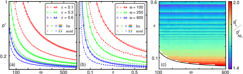
Figure 3: (color online) Critical connectivity in isolated FFNs. (a,b) Network simulations (symbols) agree well with analytical predictions (lines) (30) and (45). The critical connectivity decays with layer size and coupling strength. (c) The reduction factor $c=p_{\text{L}}^{\ast}/p_{\text{NL}}^{\ast}>1$ shows that nonlinear dendritic interaction compensates for reduced connectivity. In both scenarios, with linear and nonlinear coupling, we find that $p^{\ast}\propto\omega^{-1}$, such that the reduction factor is independent of the layer size. In networks with linear couplings the critical connectivity is $p^{\ast}\propto\epsilon^{-1}$, whereas in networks with nonlinear coupling the dependence on $\epsilon^{-1}$ is nonlinear. Therefore the reduction factor increases with decreasing coupling strength. Dashed horizontal lines indicate jumps in the reduction factor where the number of inputs needed for dendritic spike generation changes.

We now consider networks incorporating nonlinear dendritic interactions and show that and how the connectivity and number of active neurons required for propagation of synchrony is smaller. In such networks, the mechanism underlying propagation of synchrony is different, because it is supported predominantly by nonlinearly enhanced inputs. This implies that the maximal input is bounded by $\kappa$, leading to a saturation in the return map (16) (cf. Fig. 2c). The saturation enables propagating pulses of a size substantially smaller than $\omega$, in contrast to linearly coupled networks. The discontinuity in the modulation function $\sigma$ induces a discontinuity in $p_{f}\left(\sigma\left(x\right)\right)$ which prevents our previous analytical method. We thus determine the critical connectivity by a self-consistency approach. When a synchronous pulse arrives at a specific layer, the summed excitatory input strength $x$ is either smaller or larger than the dendritic threshold $\Theta_{b}$. For sufficiently small $\Theta_{b}$, the spiking probability of a neuron due to a subthreshold input is much smaller than due to a suprathreshold input, i.e. $p_{f}(\Theta_{b})\ll p_{f}(\kappa)$. Thus only a small fraction of neurons receive an input smaller than $\Theta_{b}$ and is elicited to spike. We approximate $p_{f}(x)=0$ for $x\leq\Theta_{b}$. When there is persistent propagation of synchrony, $p_{\gamma}$, which denotes the fraction of neurons that receive sufficiently strong input to reach the dendritic threshold, is constant throughout the layers. The total spiking probability of a single neuron upon the arrival of the synchronous pulse is then given by the product $p_{\gamma}p_{f}(\kappa)$. The probability

$$p^{\#}(g)=\binom{\omega}{g}\left(p_{\gamma}p_{f}(\kappa)\right)^{g}\left(p_{\gamma}p_{f}(\kappa)\right)^{\omega-g}$$ (31)

for $g$ neurons to spike synchronously follows a binomial distribution. By combining the total spiking probability and the topological connection probability $p$, we compute the probability

$$P\left(k\right) = \sum_{g=k}^{\omega}\binom{g}{k}p^{k}(1-p)^{g-k}p^{\#}(g)$$ (32)

$$= \binom{\omega}{k}\left(p_{\gamma}pp_{f}(\kappa)\right)^{k}\left(1-p_{\gamma}pp_{f}(\kappa)\right)^{\omega-k}$$ (33)

that a neuron of the subsequent layer receives exactly $k$ synchronous spikes. Thus, $k$ itself is binomially distributed and we denote its mean value by $\delta$ and its standard deviation by $\sigma_{\delta}$. Using a Gaussian approximation of the Binomial distribution yields the self-consistent equation

$$p_{\gamma} = \sum_{k=\left\lceil\Theta_{b}/\epsilon\right\rceil}^{\omega}P(k)$$ (34)

$$\approx \int_{\frac{\Theta_{b}}{\epsilon}}^{\infty}\frac{1}{\sqrt{2\pi}\sigma_{\delta}}\exp\left(-\frac{1}{2}\left(\frac{k-\delta}{\sigma_{\delta}}\right)^{2}\right)dk$$ (35)

$$= \frac{1}{2}\left(1-\mbox{Erf}\left[\frac{\frac{\Theta_{b}}{\epsilon}-\delta}{\sqrt{2}\sigma_{\delta}}\right]\right)$$ (36)

$$=: \frac{1}{2}\left(1+\mbox{Erf}\left(\frac{n}{\sqrt{2}}\right)\right),$$ (37)

where we defined

$$n := \frac{\delta-\Theta_{b}/\epsilon}{\sigma_{\delta}}$$ (38)

$$= \frac{\omega\cdot p_{\gamma}\cdot p\cdot p_{f}(\kappa)-\Theta_{b}/\epsilon}{\sqrt{\omega\cdot p_{\gamma}\cdot p_{f}(\kappa)\cdot p\cdot(1-p_{\gamma}\cdot p_{f}(\kappa)\cdot p)}}$$ (39)

as the distance between the average number of inputs and the number needed to reach the onset of the nonlinearity, measured in units of $\sigma_{\delta}$. Solving definition (38) for $p$ that occurs as an argument of $\delta$ and $\sigma_{\delta}$ and using Eq. (37) yields the connection probability in terms of $n$,

$$p_{\text{NL}}=\frac{n^{2}\epsilon+2\text{$\Theta_{b}$}+n\sqrt{n^{2}\epsilon^{2}+4\Theta_{b}\left(\epsilon-\frac{\text{$\Theta_{b}$}}{\omega}\right)}}{p_{f}(\kappa)\epsilon(n^{2}+\omega)\left(1+\mbox{Erf}\left(\frac{n}{\sqrt{2}}\right)\right)}.$$ (40)

For a certain setup of the FFN with variable connectivity, $p_{\text{NL}}\left(n\right)$ is the connectivity for which a stationary propagation of synchrony occurs with a certain $n$. Any $p_{\text{NL}}$ above the critical connectivity $p_{\text{NL}}^{\ast}$, has two preimages $n$, corresponding to the group sizes $G_{1}$ and $G_{2}$, $p_{\text{NL}}^{\ast}$ has one preimage, and any $p_{\text{NL}}$ below $p_{\text{NL}}^{\ast}$ has none, cf. Fig. 2c. Thus, $p_{\text{NL}}(n)$ has one global minimum at $n=n^{\ast}$ where $\left.\frac{dp_{\text{NL}}(n)}{dn}\right|_{n=n^{\ast}}=0$ and the critical connectivity is $p_{\text{NL}}(n^{\ast})=p_{\text{NL}}^{\ast}$.

The comparison of the results for linearly and nonlinearly coupled FFNs is particularly enlightening in the limit of large layer size ($\omega\gg 1$) and small coupling strengths ($\epsilon\ll\Theta-V^{\textsf{reset}}$). We fix the maximal input to a neuron from the previous layer, $\epsilon\omega=\text{const}$, to preserve the network state and expand Eq. (40) in a power series around $\omega\rightarrow\infty$ and $\epsilon\rightarrow 0$. Considering the leading terms we find

$$p_{\text{NL}}\approx 2\frac{\Theta_{b}+n\sqrt{\Theta_{b}\left(\epsilon-\frac{\Theta_{b}}{\omega}\right)}}{p_{f}\left(\kappa\right)\epsilon\omega\left(1+\mbox{Erf}\left(\frac{n}{\sqrt{2}}\right)\right)}.$$ (41)

We note that propagation of synchrony mediated by dendritic spikes is enabled if a sufficiently large fraction of neurons of each layer receives a total input larger or equal $\Theta_{b}$; this implies in particular $\Theta_{b}<\omega\epsilon$. Moreover, if the connectivity within the FFN is low, stable propagation even requires $\Theta_{b}\ll\omega\epsilon$ and $p_{\text{NL}}$ further simplifies to

$$p_{\text{NL}}\approx\frac{2\Theta_{b}}{p_{f}(\kappa)\epsilon\omega}\frac{1+n\sqrt{\frac{\epsilon}{\Theta_{b}}}}{1+\text{Erf}\left(\frac{n}{\sqrt{2}}\right)}.$$ (42)

As described above, the critical connectivity is given by the minimum of $p_{\text{NL}}$ as a function of $n$, which is assumed at $n=n^{*}$. $\left.\frac{dp_{\text{NL}}(n)}{dn}\right|_{n=n^{\ast}}=0$ yields $n^{*}$ as an implicit function of $\frac{\Theta_{b}}{\epsilon}$,

$$\sqrt{\frac{\Theta_{b}}{\epsilon}}=\sqrt{\frac{\pi}{2}}\exp\left(\frac{n^{\ast^{2}}}{2}\right)\left(1+\mbox{Erf}\left(\frac{n^{\ast}}{\sqrt{2}}\right)\right)-n^{\ast}.$$ (43)

For better readability, we define

$$\beta\left(\frac{\Theta_{b}}{\epsilon}\right): = \frac{1}{2}\left(1+\text{Erf}\left[\frac{n^{\ast}}{\sqrt{2}}\right]\right)-n^{\ast}\frac{e^{-\frac{n^{\ast^{2}}}{2}}}{\sqrt{2\pi}},$$ (44)

where $n^{*}=n^{*}\left(\frac{\Theta_{b}}{\epsilon}\right)$ as given by Eq. (43). Combining Eqs. (42-44) enables to simplify the critical connectivity to

$$p_{\text{NL}}^{\ast}=\frac{\Theta_{b}}{p_{f}(\kappa)\epsilon\omega}\cdot\frac{1}{\beta\left(\Theta_{b}/\epsilon\right)},$$ (45)

which depends nonlinearly on the number of spikes needed to reach the dendritic threshold ($\Theta_{b}/\epsilon$) through the function $1/\beta\left(\cdot\right)$. One can show that $\beta(\Theta_{b}/\epsilon)$ increases with decreasing coupling strength $\epsilon$ from $\beta(\Theta_{b}/\epsilon)=0.5$ for large $\epsilon$ and becomes maximal in the limit of small couplings, $\lim_{\epsilon\rightarrow 0}\beta(\Theta_{b}/\epsilon)=1$. Fig. 3 displays the results for $p_{\text{NL}}^{\ast}$ together with numerical simulations. As in the linearly coupled network the critical connectivity decays with layer size and coupling strength, but the dependence on $1/\epsilon$ is nonlinear. The factor

$$c:=\frac{p_{\text{L}}^{\ast}}{p_{\text{NL}}^{\ast}}=\frac{p_{f}(\kappa)}{\lambda\Theta_{b}}\cdot\beta\left(\frac{\Theta_{b}}{\epsilon}\right),$$ (46)

by which the nonlinear dendritic interactions reduce the required network connectivity increases with decreasing threshold $\Theta_{b}$ and increasing enhancement $\kappa$. Fig. 3c illustrates the numerically obtained reduction of connectivity: The critical connectivity $p_{\text{NL}}^{\ast}$ is smaller over the whole parameter range; the reduction is most effective for small $\epsilon$ and largely independent of $\omega$.

Nonlinear dendrites thus foster propagation of synchrony. We remark that our model still overestimates the capability of linearly coupled networks to propagate synchrony: Upon synchronous input linearly coupled groups of neurons generate synchronous output (if they generate output at all). This is a consequence of the infinitesimally short synaptic currents. In neurons with extended synaptic currents the timing of the output strongly depends on the neurons’ state and input strength. In contrast the timing of somatic action potentials elicited by dendritic spikes is largely independent thereof. We therefore expect the effect of nonlinear dendrites to be even stronger in networks of biologically more detailed neurons as considered in the next section.

III.3 Recurrent networks

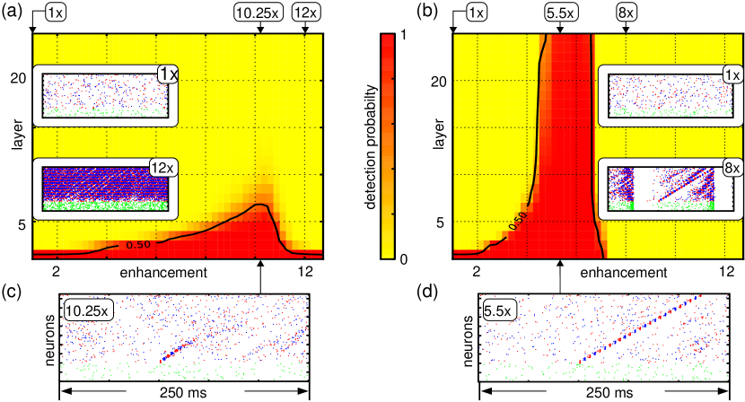
Figure 4: (color online) Nonlinear dendritic interactions enable guided propagation of synchrony in random networks ($N=10.000$, $p=0.03$, $\omega=30$). (a,b): Detection probability of induced synchronous activity in conventional networks (a) and networks with nonlinear dendrites (b). Insets of (a,b), and (c,d): Typical examples of network activity for different synaptic enhancement factors (red and blue: spikes of neurons within the FFN, green: spikes of neurons randomly sampled from the remaining neurons).

The main findings generalize in two ways, to FFNs occurring in recurrent random networks and to biologically more detailed models. For such systems, we show that in nonlinearly coupled networks stable propagation naturally emerges where it is difficult to achieve in linearly coupled networks. In contrast to isolated FFNs studied above, we now account for effects of the FFN on the surrounding network and its feedback. Further, we choose a more detailed neuron model (see section “Models and Methods”) to assure that main assumptions underlying the analytically tractable model are not crucial for stable propagation of synchrony. In particular, we show that systems with temporally extended postsynaptic responses and temporally extended nonlinear dendritic interaction window exhibit qualitatively the same phenomena as found above.

We consider networks of randomly connected conductance-based leaky integrate-and-fire neurons (cf. Eqs. (8)-(10)). The networks consist of $N^{\text{E}}$ excitatory and $N^{\text{I}}$ inhibitory neurons. A directed connection between two neurons is present with probability $p$. As for the isolated FFNs considered above, we construct the network such that the ground state in the absence of synchronous activity is characterized by balanced excitatory and inhibitory input, which results in an asynchronous irregular spiking activity. For simplicity, all neurons have the same parameters, e.g $C_{l}^{\text{m}}=C^{\text{m}}$, $g_{l}^{L}=g^{L}$, etc.

First we set up a model network, where the total excitation and inhibition to the neurons is balanced such that the spiking activity is asynchronous irregular. The external constant current $I^{0}$ determines together with the leak conductance $g^{L}$ and the resting potential $V^{\text{rest}}$ the asymptotic membrane potential in the absence of incoming spikes,

$$V^{\infty}=V^{\text{rest}}+\frac{I^{0}}{g^{L}}.$$ (47)

Additionally, each neuron receives excitatory and inhibitory random Poissonian spike trains. The frequencies are denoted by $\nu^{\text{ext,ex}}$ and $\nu^{\text{ext,in}}$ and the ratio between them is chosen such that it equals the ratio of the number of excitatory and inhibitory neurons in the network,

$$\frac{\nu^{\text{ext,ex}}}{\nu^{\text{ext,in}}}=\frac{N^{\text{E}}}{N^{\text{I}}}.$$ (48)

This ensures that each neuron receives the same ratio of excitatory and inhibitory input from both the network and external sources when neurons in the excitatory and inhibitory network populations spike on average with the same mean rate. All excitatory as well as all inhibitory connections have the same strength, i.e. $g_{lj}^{\text{max}}=g^{\text{ex}}$ for excitatory and $g_{lj}^{\text{max}}=g^{\text{in}}$ for inhibitory connections. The ratio of the peak postsynaptic potentials due to an inhibitory and an excitatory input at the asymptotic membrane potential $V^{\infty}$ is approximately given by

$$g^{\text{rat}}:=\frac{g^{\text{in}}\left|V^{\infty}-E^{\text{in}}\right|}{g^{\text{ex}}\left|V^{\infty}-E^{\text{ex}}\right|}.$$ (49)

We set

$$g^{\text{rat}} \stackrel{{\scriptstyle!}}{{=}} \frac{N^{\text{E}}}{N^{\text{I}}}=\frac{\nu^{\text{ext,ex}}}{\nu^{\text{ext,in}}}$$ (50)

$$g^{\text{in}} = \frac{\left|V^{\infty}-E^{\text{ex}}\right|}{\left|V^{\infty}-E^{\text{in}}\right|}\cdot\frac{N^{\text{E}}}{N^{\text{I}}}\cdot g^{\text{ex}}$$ (51)

to obtain balanced activity.

In contrast to the model considered in the first sections, now excitatory neurons have a non-zero time window $\Delta t$ for nonlinear dendritic modulation. When the strength of the excitatory input within $\Delta t$ exceeds a threshold, a current pulse is injected into the soma, modeling the effect of a dendritic spike. The neuron parameters for this phenomenological model are chosen according to experimental findings to reproduce the time course of the membrane potential in response to a dendritic spike quantitatively (see section “Models and Methods”).

Considering a random network we detect naturally occurring weak feed-forward-structures suitable for signal transmission in the following way: We randomly choose a group of $x$ neurons to be the first layer. The second layer is composed of $x$ neurons out of those receiving the largest numbers of connections from the initial group. By repeating this selection process $l$ times, we identify a FFN consisting of $l$ layers. In each selection step, we exclude the $x$ neurons of the previous layer, but allow to choose neurons which are members of the layers preceding the previous one. The high-connectivity subnetwork selected from an existing random network as described above by construction has a slightly higher than average connection probability. Therefore this structure is particularly well suited to enable propagation of synchrony. Alternatively one can assign neurons randomly to the different layers and compensate for smaller connectivity by, e.g., larger layer sizes according to Eq. (45).

The measurements start after an equilibration phase (initially the network is at rest). In the ground state, the network generates balanced irregular activity. Propagation of synchrony is initiated by exciting the neurons of the first layer to spike within a short time interval, which is smaller than the time window of dendritic integration, $\Delta t$. This leads to an increased input to the second layer after a delay time $\tau$. This, in turn, may lead to highly synchronous spiking of a certain number of neurons of the second layer (possibly supported by dendritic spikes) and therewith to synchronous spiking after another delay time $\tau$ in the third layer etc. Propagation of synchrony requires that (i) the total input of a layer to its successor within the FFN is sufficiently strong and (ii) that the input to the remaining network is sufficiently weak to avoid excitation of too many neurons to synchronous spiking. Requirement (ii) prevents pathological activity such as “synfire-explosions” [6].

After initiating a propagation of synchrony by exciting the neurons of the first group to spike within a short time interval, we measure the probability of detecting a synchronous pulse in the subsequent groups (see section “Models and Methods”), cf. Fig. 4a,b. Although the average connectivity within the identified FFN is significantly larger than the overall connectivity $p$, it is still small and propagation of synchronous activity is very unlikely (upper insets of Fig. 4a,b). We find that it is not sufficient to choose high-connectivity subnetworks as FFNs (as described above) to obtain a stable propagation of synchrony, but that the synapses within the FFN have to be strengthened. To study the transition to propagation we strengthen the synapses within the FFN gradually. As suggested by the results on isolated chains, we observe a propagation of synchrony over more and more layers for moderate enhancements (Fig. 4c,d). For very strong enhancements the feedback from the network becomes important: The synaptic amplification leads to an increased spontaneous activity within the FFN and this in turn results in an increased background activity. The overall increased spiking activity causes spontaneous synchronous pulses and a separation of the induced synchronous signal from the background activity is not possible anymore (the detection probability decreases, see Fig. 4a,b and lower insets).

In agreement with previous studies (cf. [7]), we find that in the linearly coupled networks considered a synchronous pulse propagates only over a few layers, even in the optimal enhancement range (Fig. 4a). In contrast, networks incorporating nonlinear dendrites support stable propagation of synchrony (Fig. 4b) in a substantial region of parameter space. In addition the propagation is enabled for enhancements considerably smaller than the optimal enhancement for networks with linear dendrites.

IV Discussion

In conclusion, we have analyzed strongly diluted networks with linear and nonlinear dendritic interactions. We have shown that and how nonlinear dendritic interactions may enhance and stabilize synchrony propagation in both isolated feed-forward chains and in recurrent network structures. Moreover, our results show that such local nonlinear interactions support the separation of propagating synchrony and asynchronous background activity. Earlier works [6, 7] did not take into account supralinear amplification of synchronous activity. There is one study [7] using existing connections in recurrent networks to create diluted chains assuming strongly enhanced synapses and at the same time specifically tuned neuron properties; still synchrony could propagate only over a few groups. In contrast, the results presented above indicate that a reliable propagation is achieved by only mildly adapted synapses and without specifically tuning or changing neuron properties or rewiring the network.

In a recent study [18] incorporating nonlinear dendrites it has been shown that synchronous activity can propagate in purely random networks without modified connections. There are no specific propagation paths but neurons are recruited in a quasi-random manner. Our results above now indicate that specific feed-forward chains that naturally occur in random neural circuits are capable of persistently propagating synchronous signals if their synaptic strengths are increased. The strengths required in the presence of nonlinear interactions are common in biological neural circuits [19] and may well be generated by learning, e.g. through spike-timing-dependent plasticity.

Dendritic (coupling) nonlinearities therefore offer a viable mechanism for guiding synchrony through weakly structured random topologies.

Recently [12] feed-forward chains with slow dendritic (probably calcium) spikes have been simulated to check the possibility of the occurrence of specific spike patterns that are experimentally observed in the higher vocal center of song birds. Our theoretical work now yields analytic insights about the collective dynamics of circuits with fast dendritic (sodium) spikes. Fast dendritic spikes have been found in the hippocampus and in the neocortex and may thus be involved in hippocampal replay, memory formation and other computational processes. Experimentally, the influence of fast dendritic spikes could be directly checked by selectively blocking dendritic sodium channels (e.g. [20] indicates that the types of sodium channels in the dendrite and soma are different) and thereby distinguishing effects coming from non-additive coupling via fast dendritic spikes from those induced by other mechanisms. During the last decade, the number of neurons simultaneously accessible has multiplied from a few to the order of $10^{2}$ neurons, with this rapid trend further ongoing. When recording the activity of a substantial fraction of neurons of a local circuit synchrony propagation should be clearly detectable and analyzable. Our results suggest that synchrony propagation and thus spike patterns should be influenced if dendritic sodium channels and thus fast dendritic spikes are blocked. Specifically, in the hippocampus, the precision of (replayed) spike patterns will decrease or the patterns vanish after blocking. Such experiments would thus provide a direct test of how non-additive coupling is exploited for the collective dynamics of neural circuits. Once the connectome, i.e. the structural synaptic connectivity, of neural circuits becomes available in the future [21], the relative impact of synaptic, structural to dynamic features of single neurons on circuit dynamics may be well distinguishable.

The basis model of pulse-coupled units considered here is applicable to a range of systems in nature, not only neural circuits but also, e.g., earthquakes emerging from abruptly relaxing tectonic plates, and fireflies interacting by exchanging light flashes (e.g. [22]). We have now studied the impact of nonlinear input modulation on collective network dynamics and derived methods for their analysis that may be useful also in a non-neuronal setting. Interestingly, very recent results [23] have shown that fireflies are more prone to respond to synchronous flashes rather than to asynchronous ones suggesting a direct application of our model.

V Acknowledgments

Supported by the BMBF (grant no. 01GQ1005B), the DFG (grant no. TI 629/3-1) and the Swartz Foundation. Simulation results were partly obtained using the simulation software NEST [24].

VI Appendix

VI.1 Parameters for Figs. 2 and 3

The single neuron parameters and the coupling delay are $\tau^{\text{m}}=1/\gamma=14$ms, $\Theta=15$mV, $V^{\text{reset}}=0$mV, $t^{\text{ref}}=2$ms and $\tau=10$ms [25, 15]. The external input is characterized by $\epsilon^{\text{ext,ex}}=-\epsilon^{\text{ext,in}}=0.5$mV [19, 27], $\nu^{\text{ext}}=\nu^{\text{ext,ex}}=\nu^{\text{ext,in}}=3$kHz and $V^{\infty}=5$mV. The parameters of the dendritic modulation function were chosen according to single neuron measurements as $\Theta_{b}=4$mV and $\kappa=11$mV [8].

The maps and transition matrices presented in Fig. 2 are derived for $\omega=100$ and $\epsilon_{ij}=\epsilon=0.3\text{mV}$. To obtain the distribution of active neurons $g_{i+1}$ in layer $i+1$, we excite $g_{i}$ neurons of the first layer to spike simultaneously and measure the number of active neurons in the following layer. For each value of $g_{i}$ we calculate the distribution for $m=1000$ different realizations of the FFN and initial conditions.

In Fig. 3, existing connections within the FFN have strengths $\epsilon_{ij}=\epsilon$. We determine the critical connectivity for $\epsilon\in\left[0.05\text{mV},0.6\text{mV}\right]$ and layer sizes $\omega\in\left[50,600\right]$ as follows: We construct a FFN consisting of $20$ layers, with $\omega$ neurons in each layer and connect neurons of successive layers with probability $p\in\left[0,1\right]$. After an equilibration time $t^{\text{init}}$ (initially the network is at rest), we initiate propagation of synchrony by exciting all neurons of the first layer to spike simultaneously. We then check whether the synchronous pulse propagates up to layer $i$, i.e. whether there is synchronous activity in layer $i$ at time $t_{i}^{\text{exp}}=t^{\text{init}}+(i-1)\cdot\tau.$ We consider the propagation for a certain setup specified by $\epsilon,$ $\omega$ and $p$ as ‘successful’, if a synchronous pulse propagates along the whole FFN in more than $50\%$ of $o=31$ realizations of the FFN with different initial conditions. We derive the critical connectivities $p_{\text{L}}^{\ast}$ and $p_{\text{NL}}^{\ast}$ up to a resolution of $\frac{\Delta p}{p}=5\cdot 10^{-3}$ by repeatedly bisecting the interval $[0,1]$ and testing the success of propagation.

VI.2 Parameters for Fig. 4

For the network simulations, we employed the simulation software NEST [24], by the NEST Initiative, available at www.nest-initiative.org. The networks had a total number of $N=10.000$ neurons with $N^{\text{E}}=8.000$ and $N^{\text{I}}=2.000$. For simplicity all neurons are considered identical, i.e. $C_{l}^{\text{m}}=C^{\text{m}}$, $g_{l}^{L}=g^{L}$, $V_{l}^{\text{rest}}=V^{\text{rest}}$, $I_{l}^{0}=I^{0}$, $\Theta_{l}=\Theta$, $t_{l}^{\text{ref}}=t^{\text{ref}}$ and $V_{l}^{\text{reset}}=V^{\text{reset}}$. The single neuron parameters are $C^{\text{m}}=400$pF, $V^{\text{rest}}=V^{\text{reset}}=-65$mV, $g^{L}=25$nS, $\Theta=-50$mV, $t^{\text{ref}}=3$ms [25, 26], $I^{0}=250$pA, and the frequencies of the external inputs are $\nu^{\text{ext,ex}}=2.4$kHz and $\nu^{\text{ext,in}}=0.6$kHz. The recurrent connectivity in cortical and hippocampal networks is sparse: Connection probabilities between $1\%$ and $10\%$, depending on the distance and the region have been estimated (e.g. [25, 19, 27]), for our simulations we choose $p=0.03$.

The time constants of the excitatory (AMPA) conductances are $\tau^{\text{A,1}}=2.5$ms and $\tau^{\text{A,2}}=0.5$ms [28]. For simplicity, we choose the same time constants for the inhibitory (GABA${}_{\text{A}}$) conductances, $\tau^{\text{G,1}}=2.5$ms and $\tau^{\text{G,2}}=0.5$ms. The reversal potentials are $E^{\text{ex}}=0$mV and $E^{\text{in}}=-75$mV [15, 25]. The strengths of experimentally observed pEPSPs due to single inputs range from small values like $0.1$mV to larger values like $2$mV [25, 19, 27]. For non-enhanced couplings, we set $g^{\text{ex}}=0.6$nS, which corresponds to a pEPSP of approximately $0.3$mV at rest. According to Eq. (51), the coupling strength of the inhibitory synapses are $g^{\text{in}}=-6.6$nS to maintain balanced input. This configuration results in an asynchronous irregular ground state with a spontaneous firing rate $\nu\approx 1.8$Hz.

The parameters of the dendritic spike current are chosen according to single neuron measurements in hippocampal cells: $\Delta t=2$ms [8], $g^{\Theta}=8.65$nS (corresponding to a pEPSP of about $3.8$mV at rest [8]), $\tau^{\text{DS}}=2.7$ms (such that $\tau+\tau_{DS}=4.7$ms and the peak of the depolarization is reached approximately $5$ms after presynaptic spiking), $A=55$nA, $B=64$nA, $C=9$nA, $\tau^{\text{DS,1}}=0.2$ms, $\tau^{\text{DS,2}}=0.3$ms, $\tau^{\text{DS,3}}=0.7$ms and $t^{\text{ref,DS}}=5.2$ms. The correction factor, which modulates the strength of the dendritic spike, is found by fitting a linear correction function, $c(g)=\max\left\{1.5-g\cdot 0.053\text{nS}^{-1},0\right\}$, such that the experimentally observed region of saturation is obtained. The dynamics of the neuron model incorporating the mechanism for dendritic spike generation is illustrated in Fig. 1.

For calculating the SNR we use an $a=0.99$ and $b=2$ and an expected width of the synchronous pulse $t^{w}=10$ms; the result is insensitive to changes in these parameters. The expected interval between successive synchronous active layers,$\Delta t^{\text{exp}}$, is chosen from the interval $\left[2\text{ms},7\mbox{\text{ms}}\right]$ such that the signal, $\sum_{i}S_{i}$, is maximized (cf. section “Models and Methods”). The control interval time interval for the estimation of the noise level is $\Delta t^{obs}=15$s. The detection probability shown in Fig. 4a,b is the fraction of successful propagations obtained from $10$ different network realizations, where for each network setup propagation of synchrony was tested for $20$ initial conditions.

All measurements start after an initial equilibrium phase of $t{}^{0}=4000$ms.

References

- [1] C. v. Vreeswijk and H. Sompolinsky, Chaos in neuronal networks with balanced excitatory and inhibitory activity, Science 274, 1724 (1996).
- [2] N. Brunel, Dynamics of sparsely connected networks of excitatory and inhibitory spiking neurons, J. Comput. Neurosci. 8, 183 (2000).
- [3] S. Jahnke, R.-M. Memmesheimer, and M. Timme, Stable irregular dynamics in complex neural networks, Phys. Rev. Lett. 100, 048102 (2008); S. Jahnke, R.-M. Memmesheimer, and M.Timme, How chaotic is the balanced state?, Front. Comp. Neurosci. 3, 13 (2009).
- [4] M. London, A. Roth, L. Beeren, M. Häusser, and P. Latham, Sensitivity to perturbations in vivo implies high noise and suggests rate coding in cortex, Nature 466, 123 (2010).
- [5] M. Abeles, Local Cortical Circuits: An Electrophysiological Study, Springer, Berlin (1982); M. Diesmann, M.-O. Gewaltig, and A. Aertsen, Stable propagation of synchronous spiking in cortical neural networks, Nature 402, 529 (1999).
- [6] C. Mehring, U. Hehl, M. Kubo, M. Diesmann, and A. Aertsen, Activity dynamics and propagation of synchronous spiking in locally connected random networks, Biol. Cybern. 88, 395 (2003); Y. Aviel, C. Mehring, and D. Horn, On embedding synfire chains in a balanced network, Neural Comput 15, 1321 (2003); A. Kumar, S. Rotter, and A. Aertsen, Conditions for Propagating Synchronous Spiking and Asynchronous Firing Rates in a Cortical Network Model, J. Neurosci. 28, 5268 (2008).
- [7] T. Vogels and L. Abbott, Signal Propagation in Networks of Integrate-and-Fire Neurons, J. Neurosci. 25, 10786 (2005).
- [8] G. Ariav, A. Polsky, and J. Schiller, Submillisecond precision of the input-output transformation function mediated by fast sodium dendritic spikes in basal dendrites of CA1 pyramidal neurons, J. Neurosci. 23, 7750 (2003); S. Gasparini, M. Migliore, and J.C. Magee, On the initiation and propagation of dendritic spikes in CA1 pyramidal neurons, J. Neurosci. 24, 11046 (2004); A. Polsky, B.W. Mel, and J. Schiller, Computational subunits in thin dendrites of pyramidal cells, Nat. Neurosci. 7, 621 (2004); S. Gasparini and J.C. Magee, State-dependent dendritic computation in hippocampal CA1 pyramidal neurons, J. Neurosci. 26, 2088 (2006).
- [9] M. Häusser, N. Spruston, and G. Stuart, Diversity and dynamics of dendritic signaling, Science 290, 739 (2000).
- [10] B. Mel, The clusteron: Toward a simple abstraction for a complex neuron, Advances in neural information processing systems (NIPS) 4 (1991); B. Mel, Why have dendrites? A computational perspective, in Dendrites (2nd edition), edited by G. Stuart et. al, Oxford University Press (2007); P. Poirazi, T. Brannon, and B. Mel, Arithmetic of subthreshold synaptic summation in a model CA1 pyramidal cell, Neuron 37, 989 (2003).
- [11] R. Traub and R. Wong, Cellular mechanism of neuronal synchronization in epilepsy, Science 216, 745 (1982); D. Jin, F. Ramazanoglu, and H. Seung, Intrinsic bursting enhances the robustness of a neural network model of sequence generation by avian brain area HVC, J. Comp. Neurosc. 23, 283 (2007).
- [12] M. Long, D. Jin, and M. Fee, Support for a synaptic chain model of neuronal sequence generation, Nature 468, 394 (2010).
- [13] S. Jahnke, R.-M. Memmesheimer, and M. Timme, in preparation.
- [14] R.-M. Memmesheimer, Quantitative prediction of intermittent high-frequency oscillations in neural networks with supralinear dendritic interactions, Proc. Natl Acad. Sci. U.S.A 107, 11092, (2010).
- [15] P. Dayan and L. Abbott, TheoreticalNeuroscience: Computational and Mathematical Modeling of Neural Systems, MIT Press, Cambridge (2001).
- [16] N. Brunel and V. Hakim, Fast global oscillations in networks of integrate-and-fire neurons with low firing rates, Neural Comput. 11, 1621 (1999); M. Helias, M. Deger, S. Rotter, and M. Diesmann, Instantaneous non-linear processing by pulse-coupled threshold units, PLoS Comput. Biol. 6, e1000929 (2010).
- [17] M. Abeles, G. Hayon, and D. Lehmann, Modeling compositionality by dynamic binding of synfire chains, J. Comp. Neurosci. 17, 179 (2004); S. Goedeke and M. Diesmann, The mechanism of synchronization in feed-forward neuronal networks, New J. Phys. 10, 015007 (2008).
- [18] R.-M. Memmesheimer, and M. Timme, Non-additive coupling enables propagation of synchronous spiking activity in purely random networks, PLoS Comput. Biol. 8, e1002384 (2012)
- [19] C. Holmgren, T. Harkany, B. Svennenfors, and Y. Zilberter, Pyramidal cell communication within local networks in layer 2/3 of rat neocortex, J. Physiol. 551, 139 (2003); S. Song, P. Sjöström, M. Reigl, S. Nelson, and D. Chklovskii, Highly nonrandom features of synaptic connectivity in local cortical circuits, PLoS Biology 3, e68 (2005).
- [20] N. Golding, W. Kath, and N. Spruston, Dichotomy of action-potential backpropagation in CA1 pyramidal neuron dendrites, J. Neurophysiol. 86, 2998 (2001); V. Menon, N. Spruston, and W. Kath, A state-mutating genetic algorithm to design ion-channel models, Proc. Natl Acad. Sci. U.S.A. 106, 16829 (2009).
- [21] S. Smith, Circuit reconstruction tools today, Curr. Opin. Neurobiol. 17, 601 (2007); J. Lichtman, J. Livet, and J. Sanes, A technicolour approach to the connectome, Nature Rev. Neurosci. 9, 417 (2008).
- [22] R. Mirollo and S. Strogatz, Synchronization of pulse-coupled biological oscillators, SIAM J. Appl. Math 50, 1645 (1990); A. Herz and J. Hopfield, Earthquake cycles and neural reverberations: Collective oscillations in systems with pulse-coupled threshold elements, , Phys. Rev. Lett. 75, 1222 (1995).
- [23] A. Moiseff and J. Copeland, Firefly synchrony: a behavioral strategy to minimize visual clutter, Science 329, 181 (2010).
- [24] M.-O. Gewaltig and M. Diesmann, NEST (Neural Simulation Tool), Scholarpedia 2, 1430 (2007).
- [25] P. Andersen, R. Morris, D. Amaral, T. Bliss, and J. O’Keefe, The Hippocampus Book, Oxford University Press, Oxford (2007).
- [26] N. Staff,H. Jung,T. Thiagarajan, M. Yao, and N. Spruston, Resting and active properties of pyramidal neurons in subiculum and CA1 of rat hippocampus, J. Neurophysiol. 84, 2398 (2000).
- [27] R. Miles and R.K. Wong, Excitatory synaptic interactions between CA3 neurones in the guinea-pig hippocampus, J. Physiol. 373, 397 (1986); J. Deuchars and A.M. Thomson, CA1 pyramid-pyramid connections in rat hippocampus in vitro: dual intracellular recordings with biocytin filling, Neuroscience 74, 1009 (1996).
- [28] P. Jonas, G. Major, and B. Sakmann, Quantal components of unitary EPSCs at the mossy fibre synapse on CA3 pyramidal cells of rat hippocampus, J. Physiol. 472, 615 (1993); G. Liu and R.W. Tsien, Properties of synaptic transmission at single hippocampal synaptic boutons, Nature 375, 404 (1995).