An improved maximal inequality for 2D fractional order Schrödinger operators

Abstract.

The local maximal inequality for the Schrödinger operators of order $\alpha>1$ is shown to be bounded from $H^{s}(\mathbb{R}^{2})$ to $L^{2}$ for any $s>\frac{3}{8}$. This improves the previous result of Sjölin on the regularity of solutions to fractional order Schrödinger equations. Our method is inspired by Bourgain’s argument in case of $\alpha=2$. The extension from $\alpha=2$ to general $\alpha>1$ confronts three essential obstacles: the lack of Lee’s reduction lemma, the absence of the algebraic structure of the symbol and the inapplicable Galilean transformation in the deduction of the main theorem. We get around these difficulties by establishing a new reduction lemma at our disposal and analyzing all the possibilities in using the separateness of the segments to obtain the analogous bilinear $L^{2}-$estimates. To compensate the absence of Galilean invariance, we resort to Taylor’s expansion for the phase function. The Bourgain-Guth inequality in [BG] is also rebuilt to dominate the solution of fractional order Schrödinger equations.

1. Introduction and the main result

For $\alpha>1$, we define the $\alpha$-th order Schrödinger evolution operator by

$$U(t)f(x)\mathrel{\mathop{=}^{\rm def}}(2\pi)^{-\frac{d}{2}}\int_{\mathbb{R}^{d}}e^{i[\,x\cdot\xi+t\,|\xi|^{\alpha}]}\widehat{f}(\xi)\,d\xi,$$

and consider the following local maximal inequality

$$\Bigl{\|}\sup_{0<t<1}|U(t)f|\Bigr{\|}_{L^{2}(B(0,1))}\leq C_{\alpha,s,d}\|f\|_{H^{s}(\mathbb{R}^{d})},\;s\in\mathbb{R}\,,$$ (1)

where $H^{s}(\mathbb{R}^{d})$ is the usual inhomogeneous Sobolev space defined via Fourier transform, and $B(0,1)$ is the unit ball centered at the origin. As a consequence of (1), we have the following point-wise convergence phenomenon from a standard process of approximation and Fatou’s lemma

$$\lim_{t\rightarrow 0}U(t)f(x)=f(x),\quad\text{a.e.}\;x,\quad\forall\,f\in H^{s}(\mathbb{R}^{d}).$$

If $s>\frac{d}{2}$, we obtain (1) immediately from Sobolev’s embedding. Thus, it is natural to ask what the minimal $s$ is to ensure $\eqref{1}$.

First of all, let us briefly review the known results about (1) in the case when $\alpha=2$. This problem was raised by Carleson in [Cr], where he answered the 1D case with $s\geq\frac{1}{4}$. This result was shown to be optimal by Dahlberg and Kenig [DK]. The higher dimensional cases of (1) were established independently by Sjölin [S] and Vega [V] with $s>\frac{1}{2}$. In particular, the result can be strengthened to $s=\frac{1}{2}$ by Sjölin [S] when $d=2$. Meanwhile, Vega [V] demonstrated that (1) fails in any dimension if $s<\frac{1}{4}$. It is then conjectured that $s\geq\frac{1}{4}$ should be sufficient for all dimensions.

The breakthrough was achieved by Bourgain [B1, B2], where he showed that (1) holds with $\alpha=2$ for some $s<\frac{1}{2}$ when $d=2$. His work was carried over and improved subsequently by many authors, including Moyua, Vargas, Vega [MVV], Tao and Vargas [TV1, TV2], Lee [L] and Shao [Sh], where the best result hitherto is $s>\frac{3}{8}$ due to Lee [L].

Previous to [B3], the results about $d\geq 3$ remained $s>\frac{1}{2}$, and $s\geq\frac{1}{4}$ was still believed to be the correct condition for (1) in every dimension. The study on this problem stagnated for several years until the recent work [B3], where the $\frac{1}{2}-$barrier was broken for all dimensions. More surprisingly, Bourgain also discovered some counterexamples to disprove the widely believed assertion on the $\frac{1}{4}-$threshold. Specifically, he showed that $s\geq\frac{1}{2}-\frac{1}{d}$ is necessary for (1) if $d\geq 4$. These examples originated essentially from an observation on arithmetical progressions.

Now, let us come to the fractional order case. Sjölin proved $\eqref{1}$ with $s=\frac{1}{2}$, $d=2$ for all $\alpha>1$ in [S]. His proof involves a $TT^{*}$ argument, which reduces the problem to a dispersive estimate of a specific oscillatory integral. After localizing the integral to the high and low frequencies, the author employed a classical result by Miyachi [M] to treat the high frequency part. The other part is estimated by means of the following inequality

$$\int_{\mathbb{R}^{2}}|y|^{-1}(1+|x-y|^{4})^{-1}dy\leq\,c\,|x|^{-1},$$

where the decay rate in the right hand side can not be improved. A crucial fact which Sjölin’s proof relied heavily on is the factor $|t(x)-t(y)|^{\frac{1}{\alpha}}$ can be canceled at the end of the computation exactly for $s=\frac{1}{2}$. This is usually referred as the Kolmogoroff-Seliverstoff-Plessner method, see [Cr] and [S] for more details. Due to these reasons, it seems very difficult to pursue Sjölin’s original approach to improve this result. In this paper, we prove

Theorem 1.1.

If $d=2$ and $\alpha>1$, then (1) is valid for all $s>\frac{3}{8}$.

Remark 1.

As noted in [B3], one may modify the method to treat a general multiplier operator $\Phi(D)$ having the property that for some constants $C,\,c>0$ and all multi-indices $\gamma$

$$|\partial^{\gamma}\Phi(\xi)|\leq\,C|\xi|^{2-|\gamma|},\quad|\nabla\Phi(\xi)|\geq c\,|\xi|.$$

However, this does not concern the fractional order case.

As a consequence, we get some improvement on the higher dimensional results by using the scheme of induction on dimensions formulated in [B3].

Corollary 1.2.

For $d\geq 3$ and $\alpha>1$, there exists a $\theta_{d}$ such that (1) is valid for all $s>\theta_{d}$ with

$$\theta_{d}=\frac{1}{2}-\sigma\Big{(}\frac{1}{2}-\theta_{d-1}\Big{)},$$

for some $\sigma\in(0,\frac{1}{2})$. In particular, $\theta_{d}<\frac{1}{2}$ for every $d\geq 2$ since $\theta_{2}<\frac{1}{2}$.

Remark 2.

This improves Theorem 2 in [S] in higher dimensions. Noting that the induction argument in [B3] is independent of the order $\alpha$, we may apply it verbatim to obtain Corollary 1.2.

As in [B3], the proof is based on the multilinear restriction theorem in [BCT]. To achieve this, an important observation introduced by Bourgain and Guth [BG] is that up to an $R^{\varepsilon}$ factor and a well behaved remainder, one successfully control the free solution of the Schrödinger equation with a summation of triple products fulfilling the transversality condition for which the multilinear restriction estimate can be used. Roughly speaking, one gains structures by losing $R^{\varepsilon}$, however this is acceptable if we do not intend to solve the end-point problem. These triple products, which we will call type I terms in Section 5, are generated by iteration with respect to scales. As a result, they are used to collect the contributions obtained at different scales. In this sense, it is also reminiscent of Wolff’s induction on scale argument in [W]. In this paper, we call this robust device as Bourgain-Guth’s inequality.

Let us take this opportunity to try to moderately clarify several points in Bourgain’s argument reserving the notations in [BG] and [B3]. Of course, we do not have the ambition to present a complete clarification of Bourgain’s treatment since that will be far beyond our reach. Instead, we focus only on the points which are directly relevant to this paper. First, a crucial input is the Bourgain-Guth inequality for oscillatory integrals from [BG]. It collects the contributions of the transversal triple products from all dyadic scales between $R^{-\frac{1}{2}}$ and one, so that we can use the multilinear restriction theorem in [BCT] to evaluate the contributions at each scale. Since we are dealing with dyadic scales in $(R^{-\frac{1}{2}},1)$, we can safely consider items from all scales by taking an $\ell^{2}$ sum losing at most a factor $\log R$. To obtain this inequality, they tactically used a “ local constant trick” in [BG] according to the following principle. By writing the oscillatory integral into trigonometric sums with variable coefficients $T_{\alpha}f(x)$, one may regard $T_{\alpha}f(x)$ as a constant on each ball of radius $K$ thanks to the uncertainty principle, where these “constants” certainly depend on the position of the ball. This heuristic point is justified by convolving $T_{\alpha}f$ with some suitable bump functions. However, to carry out further manipulations especially the iterative process, it is awkward to write it out explicitly and repeatedly. Instead of this, one prefers doing formal calculation for brevity and clarity. Based on this observation, one may insert/extract the factor $T_{\alpha}f(x)$ into/from an integral over a ball of radius $K$, or more generally over a tile in suitable shape and size. All the judgements are made according to the uncertainty principle. This simple and important observation is very efficient in simplifying various explicit calculations in the context so that the Bourgain-Guth inequality can be established in [BG] by iteration. Let us say more about the establishment of Bourgain-Guth’s inequality before turning to the argument for the Schrödinger maximal function. The brilliant novelty in [BG], which we will follow in Section 5, embodied in the way of using Bonnet-Carbery-Tao’s multiplier restriction theorem. The idea might be roughly described as after writing $Tf(x)$ into a variable coefficient trigonometric sum, one may estimate for each $x\in B_{R}$ in three different manners, where only a small portion of the members in $\{T_{\alpha}f(x)\}_{\alpha}$ would dominate the behavior of $Tf(x)$. As can be seen in [BG] and Section 5, these members correspond respectively to three different scenarios which covers all the possibilities for a particular $x\in B_{R}(0)$ to encounter. According to [BG], they are titled as non-coplanar interaction, non-transverse interaction and transverse coplanar interaction. We refer to Section 5 for more detailed discussions about this classifications. Now we turn to Bourgain’s treatment on Schrödinger maximal function. The idea is that by using Bourgain-Guth’s inequality, one is reduced to controlling each item in the $\ell^{2}$ summation with desired bound. To achieve this, one tiles $\mathbb{R}^{3}$ with translates of polar sets of the cap $\tau$, which contains a triple of transversal subcaps $\tau_{1},\tau_{2},\tau_{3}$. This provides a decomposition of $B_{R}\subset\mathbb{R}^{3}$. Invoking the local constant principle, one may raise and lower the moment exponents on each tile so that the favorite trilinear restriction in [BCT] can be used. During this calculation, Galilean’s transform is employed to shift the center of the square where the frequency is localized to the center. Although we have compressed Bourgain’s argument into as few words as possible, it is far more difficult and subtle in concrete manipulations as in [B3, BG]. We confine ourselves with this brief investigation on Bourgain’s approach and turn to our situation below.

To use the strategy in [B3], we need rebuild the Bourgain-Guth inequality for general $\alpha>1$. Although this inequality is invented in [BG] for $\alpha=2$, it is rather non-trivial to generalize this result to $\alpha>1$ as will be seen in Section 5. One of the obstructions is the absence of the algebraic structure of $|\xi|^{\alpha}$ when $\alpha$ is not an integer. This fact leads to the distinctions of our argument from [B3] and [BG] in almost every aspects, especially in the proof of the bilinear $L^{2}-$estiamte in Subsection 5.2 where we introduce a new argument.

Besides the reestablishment of Bourgain-Guth’s inequality, we need a fractional order version of Lee’s reduction lemma in [L] for general $\alpha>1$. In Section 4, we establish this result using a different method. This extends the result in [L] to a more general setting. We will use the method of stationary phase in spirit of [Sh]. However, to justify the proof, we involve a localization argument which eliminates Schwartz tails by losing $R^{\varepsilon}$. To be precise, we separate the Poisson summation to a relatively large and small scales, where either the rapid decreasing property of Schwartz functions or the stationary phase argument can be used to handle the error terms. This principle is also used in the proof of the main theorem. The essence of this argument is exploiting the orthogonality in “phase space” via stationary phase and Poisson summation formula. In doing this, one only needs to afford an $R^{\varepsilon}$ loss but one may sum the pieces that are well-estimated efficiently. See Section 3 and Section 4 for more details.

At the end of this section, let us say a word about the potential of Bourgain-Guth’s approach to oscillatory integrals. In doing harmonic analysis, one of the most important principles is that structures are favorable conditions to help us use deep results in mathematics. For instance, Whitney’s decomposition was employed by the authors in [TV1, TV2, TVV] to generate the transversality conditions for the use of bilinear estimates. On the other hand, the proof of Bourgain and Guth’s inequality enlightened a new approach to generate structures by means of logical classification, i.e. exploiting the intrinsic structures implicitly involved in the the summation of large number of elements creatively using logical division. The idea is fairly new and the argument is really a tour de force, bringing in ideas and techniques from combinatorics as will be seen in Section 5. We believe this approach is very promising to get improvements on the open questions in classical harmonic analysis. In particular, the result in this paper might be improved further by refining this method.

This paper is organized as follows. In Section 2, we introduce some preliminaries and the basic lemmas. In Section 3, we prove the main result. Section 4 is devoted to the proof of Lemma 2.5 and Section 5 is devoted to the proof of Lemma 2.3.

2. Preliminaries

This section includes the list of the frequently used notations, the statement of the crucial lemma which plays the key role in deducing the main result as well as the primary reduction for the proof of Theorem 1.1.

2.1. Notations

Throughout this paper the following notations will be used.
$\diamond$ $\Omega=[-1/2,1/2]\times[-1/2,1/2]$
$\diamond$ $[r]$ is the greatest integer not exceeding $r$.
$\diamond$ If $\Omega$ is a subset of $\mathbb{R}^{d}$, we define $\displaystyle\Omega^{c}=\mathbb{R}^{d}\setminus\Omega$.
$\diamond$ $\chi_{\Omega}$ denotes the characteristic function of a set $\Omega\subset\mathbb{R}^{d}$.
$\diamond$ Suppose $\xi$ is a vector in $\mathbb{R}^{d}$, we define $\overline{\xi}=\frac{\xi}{|\xi|}$.
$\diamond$ We define $\mathcal{I}=\{\xi\in\mathbb{R}^{d}\mid 1/2\leq|\xi|\leq 2\}$ and, except Lemma 2.5 below, we always assume $d=2$.
$\diamond$ For $f(x)$ a measurable function and $a\in\mathbb{R}^{d}$, we define $\displaystyle\tau_{a}f(x)=f(x-a)$.
$\diamond$ Denote by $\mathcal{S}(\mathbb{R}^{d})$ the Schwartz class on $\mathbb{R}^{d}$ and by $\mathcal{S}^{\prime}(\mathbb{R}^{d})$ the space of tempered distributions.
$\diamond$ We use $\mathcal{F}_{x\rightarrow\xi}f$ or $\widehat{f}(\xi)$ to denote the Fourier transform of a tempered distribution $f(x)$ and

$$\widehat{f}(\xi)=(2\pi)^{-\frac{d}{2}}\int_{\mathbb{R}^{d}}f(x)e^{-ix\cdot\xi}dx.$$

$\diamond$ Denote by $B(a,K)$ or $B_{a,K}$ a ball centered at $a$ in $\mathbb{R}^{d}$ of radius $K$.
$\diamond$ Suppose $B$ is a convex body in $\mathbb{R}^{d}$ and $\lambda>0$, we use $\lambda B$ to denote the convex set having the same center with $B$ but enlarged in size by $\lambda.$
$\diamond$ The capital letter $C$ stands for a constant which might be different from line to line and $c\ll C$ means $c$ is far less than $C$. This is clear in the context.
$\diamond$ The notion $A\lesssim B$ means $A\leq CB$ for some constant $C$, and $A\simeq B$ means both $A\lesssim B$ and $B\lesssim A$.
$\diamond$ By $A\lesssim_{\eta,\zeta,\ldots}B$, we mean there is a constant $C=C(\eta,\zeta,\ldots)$ depending on $\eta,\zeta,...$ such that $A\leq CB$, where the reliance of $C$ on the parameters will be clear from the context.
$\diamond$ By $\zeta=\mathcal{O}_{\alpha}(\eta)$, we mean there is an estimate $\zeta\lesssim_{\alpha}\eta$.

2.2. Caps, tiles and the Bourgain-Guth inequality

Now we introduce some terminologies. Let $R\gg 2^{5\alpha}>1$ and $\frac{1}{\sqrt{R}}<\delta<1$. Partition $\mathbb{R}^{2}$ into $\cup_{\tau}\Omega_{\tau}$ where $\Omega_{\tau}$ is a $\delta\times\delta$ square centered at $\xi_{\tau}\in\delta\mathbb{Z}^{2}$ such that the edges of $\Omega_{\tau}$ are parallel to the abscissas and vertical axis respectively. Let $\overrightarrow{n}_{\tau}$ be the exterior unit normal vector of the immersed surface $(\xi,\,|\xi|^{\alpha})$ at the point $(\xi_{\tau},\,|\xi_{\tau}|^{\alpha})$. We define the following sets

$$\Pi^{\delta}_{\tau} =(\xi_{\tau},\,|\xi_{\tau}|^{\alpha})+\left\{z\in\mathbb{R}^{3}\mid|\langle z,\overrightarrow{n}_{\tau}\rangle|\leq\delta^{\alpha}\right\},$$

$$\mathcal{C}_{\tau} =\Pi^{\delta}_{\tau}\cap\left\{z\in\mathbb{R}^{3}\mid\,z=(z_{1},z_{2},z_{3}),\,(z_{1},\,z_{2})\in\Omega_{\tau}\right\}.$$

Obviously,  $\mathcal{C}_{\tau}$ is a parallelopiped with dimensions $\sim\delta,\,\delta,\,\delta^{\alpha}$.

Definition 2.1.

The parallelopiped $\mathcal{C}_{\tau}$ is called a $\delta-$cap associated to $\Omega_{\tau}$.

Definition 2.2.

The polar set of $\mathcal{C}_{\tau}$ is defined as

$$\mathcal{C}^{*}_{\tau}=\Bigl{\{}z\in\mathbb{R}^{3}\;\Big{|}\;|\langle z,\,w\rangle|\leq 1,\,\forall\,w\in\mathcal{C}_{\tau}-(\xi_{\tau},\,|\xi_{\tau}|^{\alpha})\Bigr{\}},$$

It is easy to see that $\mathcal{C}^{*}_{\tau}$ is essentially a $\frac{1}{\delta}\times\frac{1}{\delta}\times\frac{1}{\delta^{\alpha}}$-rectangle centered at the origin, with the longest side in the direction of $\overrightarrow{n}_{\tau}$. Moreover, we may tile $\mathbb{R}^{3}$ with boxes of the translations of $\mathcal{C}^{*}_{\tau}$. This decomposes $\mathbb{R}^{3}$ naturally into the union of essentially disjoint $\mathcal{C}^{*}_{\tau}-$boxes. We call this decomposition a tiling of $\mathbb{R}^{3}$ with $\mathcal{C}^{*}_{\tau}-$boxes. Define an oscillatory integral by

$$Tf(x)=\int_{\mathcal{I}}e^{i[x_{1}\xi_{1}+x_{2}\xi_{2}+x_{3}|\xi|^{\alpha}]}\widehat{f}(\xi)\,d\xi,$$

where $x=(x_{1},\,x_{2},\,x_{3})\in\mathbb{R}^{3}$ and $\xi=(\xi_{1},\xi_{2})\in\mathbb{R}^{2}$. Setting $x^{\prime}=(x_{1},x_{2})$ and regarding $x_{3}$ as the temporal variable $t=x_{3}$, we have

$$U(t)f(x^{\prime})=Tf(x).$$ (2)

Remark 3.

The notion in (2) for general $d-$dimensional counterpart is defined in the same way, with $x_{d+1}$ in place of $x_{3}$, and $(x_{1},x_{2})$ as well as $(\xi_{1},\xi_{2})$ replaced by $(x_{1},\ldots,x_{d})$ and $(\xi_{1},\ldots,\xi_{d})$. This will only be used for Lemma 2.5 below, which is proved for general dimensions.

Now we can state Bourgian-Guth’s inequality which will be used to control the oscillatory integral $Tf(x)$ in terms of $\{Tf_{\tau}\}_{\tau}$, where $\widehat{f}_{\tau}$ is supported in a much smaller region $\Omega_{\tau}\subset\mathcal{I}$.

Lemma 2.3.

If $\text{supp}\widehat{f}\subset\mathcal{I}$ and $1\ll K\ll R$, then for any $\varepsilon>0$ we have the following estimate on the cylinder $B(0,R)\times[0,R]\subset\mathbb{R}^{2+1}$

$$|Tf(x)| \lesssim R^{\varepsilon}\max_{\frac{1}{K}\geq\delta>\frac{1}{\sqrt{R}}}\max_{\mathcal{E}_{\delta}}\biggl{[}\sum_{\Omega_{\tau}\in\mathcal{E}_{\delta}}\Bigl{(}\psi_{\tau}\,\prod^{3}_{j=1}|Tf_{\tau_{j}}|^{\frac{1}{3}}\Bigr{)}^{2}\biggr{]}^{1/2}$$ (3)

$$\quad\quad+R^{\varepsilon}\max_{\mathcal{E}_{\frac{1}{\sqrt{R}}}}\bigg{[}\sum_{\Omega_{\tau}\in\mathcal{E}_{\frac{1}{\sqrt{R}}}}\Bigl{(}\psi_{\tau}\,|Tf_{\tau}|\Bigr{)}^{2}\bigg{]}^{1/2},$$ (4)

where $\widehat{f}_{\tau_{j}}$ is supported in $\Omega_{\tau_{j}}$ for $j=1,\,2,\,3$, and

• $\mathcal{E}_{\delta}$ consists of at most $\left(\frac{1}{\delta}\right)^{1+\varepsilon}$ disjoint $\delta\times\delta$ squares $\Omega_{\tau}$;

• $\{\Omega_{\tau_{j}}\}^{3}_{j=1}$ is a triple of non-collinear $\frac{\delta}{K}\times\frac{\delta}{K}$ squares inside $\Omega_{\tau}$;

• For each $\tau$, $\psi_{\tau}$ is a non-negative function on $\mathbb{R}^{3}$ which is constant on unit cubes and satisfies

  $$\frac{1}{|B|}\int_{B}\psi^{4}_{\tau}(x)dx\lesssim R^{\varepsilon},$$ (5)

  for all $B$ taken in a tiling of $\mathbb{R}^{3}$ with $\mathcal{C}^{*}_{\tau}-$boxes.

Remark 4.

A triplet $\bigl{(}\Omega_{\tau_{1}},\,\Omega_{\tau_{2}},\,\Omega_{\tau_{3}}\bigr{)}$ in $\Omega_{\tau}$ is said to be non-collinear if

$$|\xi_{\tau_{1}}-\xi_{\tau_{2}}|\geq|\xi_{\tau_{1}}-\xi_{\tau_{3}}|\geq\text{dist}\left(\xi_{\tau_{3}},\,\ell(\xi_{\tau_{1}},\xi_{\tau_{2}})\right)>10^{3}\frac{\alpha 2^{\alpha}}{K},$$ (6)

where $\xi_{j}$ is the center of $\Omega_{\tau_{j}}$ for $j=1,\,2,\,3$. Consequently, the caps $\mathcal{C}_{\tau_{1}},\,\mathcal{C}_{\tau_{2}},\,\mathcal{C}_{\tau_{3}}$ are transversal, that is, the exterior normal vectors associated to these three caps are linearly independent, uniformly with respect to the variables belonging to $\Omega_{\tau_{j}}$ for $j=1,2,3$. We refer to [BCT] for the precise description of the transversality condition, see also Section 3. This condition is ready for the multi-linear restriction estimate established in [BCT], as frequently used in [B3, BG].

Remark 5.

This lemma is established in the spirit of Bourgain and Guth, where it differs from [BG] in two aspect. First, the non-collinear condition is reformulated in (6) to handle general $\alpha>1$. Second, the scales of the caps and dual caps have depended on $\alpha$ already. The absence of the algebraic structure of the symbol $|\xi|^{\alpha}$ for general $\alpha>1$ will lead to some difficulties in the deduction of (3) (4) as well as the application of this inequality to the proof of Theorem 1.1. These obstacles make our argument more complicated than [B3].

Remark 6.

If $\widehat{f}_{\tau}$ is supported in a square $\Omega_{\tau}$ of size $\delta$, $|Tf_{\tau}|(x)$ can be regarded essentially as a constant on each $\mathcal{C}^{*}_{\tau}-$box. We call this the local constancy property indicated in [BG].

The advantage of this inequality allows us to gain the transversality condition in each term of the summation (3) by losing only an $R^{\varepsilon}$ factor. This is favorable especially in proving some non-endpoint estimates. We also point out that the precise cardinality of $\mathcal{E}_{\delta}$ will not be used in the proof of Theorem 1.1. We will prove Lemma 2.3 in Section 5.

2.3. A primary reduction of the problem

By Littlewood-Paley’s theory, Sobolev embedding and Hölder’s inequality, Theorem 1.1 amounts to showing for any $\varepsilon>0$, there is a $C_{\alpha,\varepsilon}$ such that

$$\Bigl{\|}\sup_{0<x_{3}<1}|Tf(\cdot,x_{3})|\Bigr{\|}_{L^{2}(B(0,1))}\leq C_{\alpha,\,\varepsilon}\,R^{\frac{3}{8}+\varepsilon}\|f\|_{2},$$ (7)

for $\widehat{f}(\xi)$ supported in $\{\xi\in\mathbb{R}^{2}\mid R/2\leq|\xi|\leq 2R\}$ with $R$ large enough.

After a re-scaling, we reduce (7) to

$$\Bigl{\|}\sup_{0<x_{3}<R^{\alpha}}|Tf(\cdot,x_{3})|\Bigr{\|}_{L^{2}(B(0,R))}\leq C_{\alpha,\varepsilon}\,R^{\frac{3}{8}+\varepsilon}\|f\|_{2},\quad\text{supp}\widehat{f}\subset\mathcal{I}.$$ (8)

When $\alpha=2$, it is observed by Lee [L] that to get (8), it suffices to prove it with the supremum taken only for $0<x_{3}<R$. This fact simplifies the problem significantly so that the result of $s>\frac{3}{8}$ can be deduced for $d=2$. This reduction is also necessary for the argument in [B3]. We extend this result to all $\alpha>1$ by proving the following lemma.

Lemma 2.4.

Suppose for any $\varepsilon>0$, there exists some $C_{\varepsilon}>0$ such that

$$\Bigl{\|}\sup_{0<x_{3}<R}|Tf(\cdot,x_{3})|\Bigr{\|}_{L^{2}(B(0,R))}\leq C_{\varepsilon}R^{\frac{3}{8}+\varepsilon}\|f\|_{2},$$ (9)

for $R$ sufficient large and $\text{supp}\widehat{f}\subset\{\xi\in\mathbb{R}^{2}\mid\frac{3}{8}\leq|\xi|\leq\frac{17}{8}\}$. Then (8) holds.

Remark 7.

Intuitively, one might expect that the interval over which the supremum is taken for $x_{3}$ in (9) should be $(0,\,R^{\frac{\alpha}{2}})$. Although this can be deduced easily by modifying our argument slightly, we will lose more derivatives in Theorem 1.1 if we use (9) with $0<x_{3}<R^{\frac{\alpha}{2}}$. The loss of derivatives forces the $s$ in (1) relies heavily on $\alpha$ and this will confine $\alpha$ in a small range in order to improve Sjölin’s result. However, our result can be strengthened so that $s$ is independent of $\alpha$ thanks to Lemma 2.4. We point out that the global maximal inequality is $\alpha-$dependent. See [R] for details.

Remark 8.

Heuristically speaking, the idea behind this lemma can be interpreted in terms of the propagation speed. If the frequency of the initial data $f$ is localized at $\mathcal{I}$, then the propagation speed of $U(t)f$ can be morally regarded as finite. Suppose $R$ is large enough so that $f$ is mainly concentrated in the ball $B(0,\,R)$. If one waits at a position in $B(0,\,R)$ for the maximal amplitude of the solution during the time period $0<t<R^{\alpha}$ to occur, then by the finite speed of propagation, this maximal amplitude can be expected to happen before the time at $R$. This heuristic intuition is justified by the following lemma.

Lemma 2.5.

Let $\displaystyle\text{supp}\,\widehat{f}(\xi)\subset\mathcal{I}$ and $j=0,1,\ldots,[R^{\alpha-1}]$, $t_{j}=jR$. Set $I_{j}=[t_{j},\,t_{j+1})$ for $j<[R^{\alpha-1}]$ and $I_{[R^{\alpha-1}]}=[t_{[R^{\alpha-1}]},R^{\alpha})$. Denote $x=(x^{\prime},x_{d+1})$ where $x^{\prime}=(x_{1},\ldots,x_{d})$ and take a smooth function $\varphi\in C^{\infty}_{0}(B(0,\,2R))$ so that $\varphi(x^{\prime})=1$ on the ball $B(0,\,R)$. Then for any $\varepsilon>0$, there is a $C_{\alpha,\,\varepsilon}>0$ and a family of functions $\{f_{j}\}_{j}$ satisfying

$$\text{supp}\widehat{f}_{j}\subset\Bigl{\{}\xi\in\mathbb{R}^{d}\,\Big{|}\;\frac{1}{2}-\frac{1}{R}\leq|\xi|\leq 2+\frac{1}{R}\Bigr{\}}\mathrel{\mathop{=}^{\rm def}}\mathcal{I}_{\frac{1}{R}},$$

so that for $x_{d+1}\in I_{j}$,

$$\varphi(x^{\prime})Tf(x)=\varphi(x^{\prime})\chi_{I_{j}}(x_{d+1})Tf_{j}(x^{\prime},\,x_{d+1}-t_{j})+\mathcal{O}_{\alpha,\varepsilon}(R^{-99d}\|f\|_{2}),$$ (10)

or equivalently, viewing $x_{d+1}=t\in I_{j}$,

$$\varphi(x^{\prime})U(t)f(x^{\prime})=\varphi(x^{\prime})\chi_{I_{j}}(t)U(t-t_{j})f_{j}(x^{\prime})+\mathcal{O}_{\alpha,\varepsilon}(R^{-99d}\|f\|_{2}),$$ (11)

Moreover, there exists a positive constant $c_{d}>0$ such that

$$\Bigl{\|}\Bigl{(}\sum^{[R^{\alpha-1}]}_{j=0}|f_{j}|^{2}\Bigr{)}^{\frac{1}{2}}\Bigr{\|}_{2}\leq\,C_{\alpha,\,\varepsilon}\,R^{\varepsilon c_{d}}\|f\|_{2}.$$ (12)

To prove this lemma, we introduce a localization argument which allows us to regard a Schwartz function with compact Fourier frequencies as a smooth cut-off function by losing $R^{\varepsilon}$. That is why we have to lose $R^{\varepsilon c_{d}}$ in (12), but this is adequate for our purpose.

Remark 9.

In our proof, $f_{j}$ is constructed by localizing $Tf(x,t_{j})$ with Schwartz functions. This leads to a loss of $\frac{1}{R}-$enlargement of $\mathcal{I}$ in the frequency space, but this does not affect the use of this lemma.

We end up this section by showing Lemma 2.4 follows from Lemma 2.5.

Proof of Lemma 2.4.

In view of (11), we have for $d=2$

$$\varphi(x^{\prime})|Tf(x^{\prime},x_{3})|\lesssim_{\alpha,\varepsilon}\varphi(x^{\prime})\sum^{[R^{\alpha-1}]}_{j=0}|\chi_{I_{j}}(x_{3})Tf_{j}(x^{\prime},x_{3}-t_{j})|+R^{-198}\|f\|_{2}.$$

Choosing $R$ large enough and neglecting $R^{-198}\|f\|_{2}$, we obtain

$$\sup_{0<x_{3}<R^{\alpha}}|\varphi(x^{\prime})Tf(x)|^{2}\lesssim_{\alpha,\varepsilon}\sum^{[R^{\alpha-1}]}_{j=0}\sup_{0<x_{3}-t_{j}<R}|\varphi(x^{\prime})Tf_{j}(x^{\prime},x_{3}-t_{j})|^{2}.$$

Integrating both sides of the above inequality on $B(0,\,R)$, we may estimate the left side of (8) by

$$\Bigl{(}\sum^{[R^{\alpha-1}]}_{j=0}\Bigl{\|}\sup_{0<x_{3}-t_{j}<R}|\varphi(x^{\prime})Tf_{j}(x^{\prime},x_{3}-t_{j})|\Bigr{\|}^{2}_{2}\Bigr{)}^{\frac{1}{2}}.$$

Using (9) and (12), we obtain

$$\eqref{2}\lesssim_{\alpha,\varepsilon}R^{\frac{3}{8}+\varepsilon}\|f\|_{2}.$$

∎

Remark 10.

In proving (9), we always fix an $\varepsilon>0$ first and then take $R$ large, which may depend possibly on $\varepsilon$, $\alpha$ and $\|f\|_{2}$. This allows us to eliminate as many error terms as possible by repeatedly using the localization argument.

Remark 11.

In fact, the original proof of [L, Lemma 2.1] for the classical Schrödinger equation works for the generalized case as well. Moreover, the proof of [LR, Lemma 2.1] can be used to get rid of the $\varepsilon$ loss.

3. Proof of the main result

Now we are in the position to prove Theorem 1.1. For any fixed $\varepsilon>0$, we normalize $\|f\|_{2}=1$. In light of Lemma 2.3 and 2.4, (9) amounts to obtaining the following two estimates for $R$ large enough

$$\sum_{\begin{subarray}{c}\frac{1}{\sqrt{R}}<\delta<\frac{1}{K}\\ \delta\,\text{dyadic}\end{subarray}} \Bigl{[}\sum_{\Omega_{\tau}:\delta\times\delta}\bigl{\|}\psi_{\tau}\prod^{3}_{j=1}|Tf_{\tau_{j}}|^{\frac{1}{3}}\bigr{\|}^{2}_{L^{2}(|x^{\prime}|<R)L^{\infty}(|x_{3}|<R)}\Bigr{]}^{\frac{1}{2}}\lesssim R^{\frac{3}{8}+\varepsilon},$$ (13)

$$\Bigl{[} \sum_{\Omega_{\tau}:\frac{1}{\sqrt{R}}\times\frac{1}{\sqrt{R}}}\bigl{\|}\psi_{\tau}|Tf_{\tau}|\bigr{\|}^{2}_{L^{2}(|x^{\prime}|<R)L^{\infty}(|x_{3}|<R)}\Bigr{]}^{\frac{1}{2}}\lesssim R^{\frac{3}{8}+\varepsilon},$$ (14)

where $x^{\prime}=(x_{1},\,x_{2})$ and $\Omega_{\tau}:\delta\times\delta$ refers to the partition of $\mathcal{I}_{\frac{1}{8}}$ into the union of $\delta\times\delta-$squares.

By orthogonality, it suffices to prove

$$\int_{|x^{\prime}|<R}\sup_{|x_{3}|<R}\Bigl{|}\psi_{\tau}\prod^{3}_{j=1}|Tf_{\tau_{j}}|^{\frac{1}{3}}\Bigr{|}^{2}(x^{\prime},x_{3})dx^{\prime}\lesssim_{\varepsilon}R^{\frac{3}{4}+2\varepsilon}\|f_{\tau}\|^{2}_{2},$$ (15)

and

$$\int_{|x^{\prime}|<R}\sup_{|x_{3}|<R}\bigl{(}\psi_{\tau}|Tf_{\tau}|\bigr{)}^{2}(x^{\prime},x_{3})dx^{\prime}\lesssim_{\varepsilon}R^{\frac{3}{4}+2\varepsilon}\|f_{\tau}\|^{2}_{2},$$ (16)

where $f_{\tau}$ is defined as $\widehat{f}_{\tau}=\widehat{f}\chi_{\Omega_{\tau}}$.

3.1. The proof of (15)

For brevity, we denote $G_{\tau_{1},\tau_{2},\tau_{3}}=\prod^{3}_{j=1}|Tf_{\tau_{j}}|^{\frac{1}{3}}$ in (15), where $(\tau_{1},\,\tau_{2},\,\tau_{3})$ corresponds to the squares $(\Omega_{\tau_{1}},\Omega_{\tau_{2}},\Omega_{\tau_{3}})$ with the properties in Lemma 2.3. Let $\xi^{\tau}$ be the center of $\Omega_{\tau}$. Then we may assume $\xi^{\tau}=(0,\,|\xi^{\tau}|)$ due to the invariance of (15) under orthogonal transformations. Let $\mathcal{C}_{\tau}$ be the $\delta-$cap associated to $\Omega_{\tau}$ and $\mathcal{C}^{*}_{\tau}$ be the polar set of $\mathcal{C}_{\tau}$. After tiling $B(0,R)\times[0,R]\subset\mathbb{R}^{3}$ with $\mathcal{C}^{*}_{\tau}-$boxes, we have

$$B(0,R)\times[0,R]\subset\bigcup_{k,j}B_{j,k}$$

where $B_{j,k}$ is a $\mathcal{C}^{*}_{\tau}-$box labeled by $j$ and $k$, with $j$ corresponding to the horizontal translation and $k$ to the vertical (see Figure.1). Adopting the notations in [B3], we denote the projection of each $B_{j,k}$ to the $(x_{1},\,x_{2})-$variables by $I_{j}=\pi_{x^{\prime}}(B_{j,k})$. Let $\mathcal{P}_{x^{\prime}}$ be the plane through the point $(x^{\prime},0)$ and perpendicular to the $x_{2}-$direction. We define $J^{x^{\prime}}_{k}=\pi_{x_{3}}(B_{j,k}\cap\mathcal{P}_{x^{\prime}})$. Then $|J^{x^{\prime}}_{k}|\sim\frac{1}{\delta}$ for all $x^{\prime}$ and $k$ . For $I_{j}$, it is easy to see that the length of the side in direction of $x_{1}$ is approximately $\frac{1}{\delta}$ and the side in the $x_{2}-$direction has length $\frac{1}{\delta^{\alpha}}$.

    $$x_{1} O \mathcal{P}_{x^{\prime}} x_{3} B_{j,k} J^{x^{\prime}}_{k} I_{j}=\pi_{x^{\prime}}(B_{j,k}) x_{2}$$

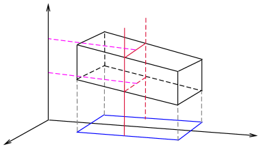
Figure 1. The $\mathcal{C}^{*}_{\tau}-$box $B_{j,k}$.

By Hölder’s inequality and the relation $\ell^{3}\hookrightarrow\ell^{\infty}$, we have

$$\sum_{j}\|\psi_{\tau}G_{\tau_{1},\,\tau_{2},\,\tau_{3}}\|^{2}_{L^{2}_{x^{\prime}}(I_{j})L^{\infty}(|x_{3}|<R)}$$

$$\leq \delta^{-\frac{1+\alpha}{3}}\sum_{j}\|\psi_{\tau}G_{\tau_{1},\,\tau_{2},\,\tau_{3}}\|^{2}_{L^{3}_{x^{\prime}}(I_{j})L^{\infty}(|x_{3}|<R)}$$

$$\leq \delta^{-\frac{1+\alpha}{3}}\sum_{j}\max_{k}\|\psi_{\tau}G_{\tau_{1},\,\tau_{2},\,\tau_{3}}\|^{2}_{L^{3}_{x^{\prime}}(I_{j})L^{\infty}_{x_{3}}(J^{x^{\prime}}_{k})}$$

$$\leq \delta^{-\frac{1+\alpha}{3}}\sum_{j}\Bigl{[}\sum_{k}\|\psi_{\tau}G_{\tau_{1},\,\tau_{2},\,\tau_{3}}\|^{3}_{L^{3}_{x^{\prime}}L^{\infty}_{x_{3}}(B_{j,k})}\Bigr{]}^{\frac{2}{3}}.$$ (17)

Using the property (5) and Remark 6, we have

$$\quad\|\psi_{\tau}G_{\tau_{1},\,\tau_{2},\,\tau_{3}}\|_{L^{3}_{x^{\prime}}L^{\infty}_{x_{3}}(B_{j,k})}$$

$$\lesssim\|\psi_{\tau}\|_{L^{3}_{x^{\prime}}L^{\infty}_{x_{3}}(B_{j,k})}\Bigl{(}\frac{1}{|I_{j}|}\int_{I_{j}}\bigl{(}\frac{1}{|J^{x^{\prime}}_{k}|}\int_{J^{x^{\prime}}_{k}}|G_{\tau_{1},\,\tau_{2},\,\tau_{3}}(x^{\prime},x_{3})|^{3}dx_{3}\bigr{)}^{\frac{2}{3}}dx^{\prime}\Bigr{)}^{\frac{1}{2}}$$

$$\lesssim|I_{j}|^{-\frac{1}{2}}|J_{k}|^{-\frac{1}{3}}\|\psi_{\tau}\|_{L^{3}_{x^{\prime}}L^{4}_{x_{3}}(B_{j,k})}\|G_{\tau_{1},\,\tau_{2},\,\tau_{3}}\|_{L^{2}_{x^{\prime}}L^{3}_{x_{3}}(B_{j,k})}$$

$$\lesssim|I_{j}|^{\frac{1}{3}-\frac{1}{4}-\frac{1}{2}}|J_{k}|^{-\frac{1}{3}}\|\psi_{\tau}\|_{L^{4}(B_{j,k})}\|G_{\tau_{1},\,\tau_{2},\,\tau_{3}}\|_{L^{2}_{x^{\prime}}L^{3}_{x_{3}}(B_{j,k})}$$

$$\lesssim\delta^{-(1+\alpha)(\frac{1}{3}-\frac{3}{4})+\frac{1}{3}}R^{\varepsilon}|B_{j,k}|^{\frac{1}{4}}\|G_{\tau_{1},\,\tau_{2},\,\tau_{3}}\|_{L^{2}_{x^{\prime}}L^{3}_{x_{3}}(B_{j,k})}$$

$$\lesssim R^{\varepsilon}\delta^{\frac{1}{4}+\frac{\alpha}{6}}\|G_{\tau_{1},\,\tau_{2},\,\tau_{3}}\|_{L^{2}_{x^{\prime}}L^{3}_{x_{3}}(B_{j,k})},$$

where, in the second inequality, we used the fact that $\psi_{\tau}$ is constant on the unit cubes. This allows us to control the $L^{\infty}$ norm of $\psi_{\tau}$ with respect to the $x_{3}$ variable on $J^{x^{\prime}}_{k}$ by $L^{4}$ norm.

Plugging this into (3.1), we get by Minkowski’s inequality

$$|\eqref{jia 1}| \lesssim\delta^{-\frac{1+\alpha}{3}}\sum_{j}\Bigl{[}\sum_{k}R^{3\varepsilon}\delta^{\frac{3}{4}+\frac{\alpha}{2}}\|G_{\tau_{1},\,\tau_{2},\,\tau_{3}}\|^{3}_{L^{2}_{x^{\prime}}L^{3}_{x_{3}}(B_{j,k})}\Bigr{]}^{\frac{2}{3}}$$

$$\lesssim R^{2\varepsilon}\delta^{\frac{1}{6}}\sum_{j}\int_{I_{j}}\Bigl{(}\sum_{k}\int_{J^{x^{\prime}}_{k}}|G_{\tau_{1},\,\tau_{2},\,\tau_{3}}|^{3}(x^{\prime},x_{3})dx_{3}\Bigr{)}^{\frac{2}{3}}dx^{\prime}$$

$$\lesssim R^{2\varepsilon}\delta^{\frac{1}{6}}\|G_{\tau_{1},\,\tau_{2},\,\tau_{3}}\|^{2}_{L^{2}(|x^{\prime}|<R)L^{3}(|x_{3}|<R)}.$$ (18)

Remark 12.

In (18), $\alpha$ is absent from the exponent of $\delta$ and $R$. However, the role of $\alpha$ is enrolled in the estimation of

$$\|G_{\tau_{1},\,\tau_{2},\,\tau_{3}}\|^{2}_{L^{2}(|x^{\prime}|<R)L^{3}(|x_{3}|<R)}.$$ (19)

To handle this expression, Bourgain used Galilean’s transformation to shift the center of the domain for the integral $Tf_{\nu}$ to the origin when $\alpha=2$. We can not directly use this due to the absence of the algebraic structure of $|\xi|^{\alpha}$ for general $\alpha>1$. To adapt his strategy, we get around this obstacle by using Taylor’s expansion. We also use a localization argument as in the proof of Lemma 2.5.

It remains to evaluate (19). Let us introduce some notations. Define

$$\mathcal{T}_{\delta,\,\tau}h(x_{1},\,x_{2},\,x_{3})=\int_{\mathbb{R}^{2}}e^{i[x_{1}\eta_{1}+x_{2}\eta_{2}+x_{3}\Phi\,(\xi^{\tau},\lambda_{0},\alpha,\delta,\eta)]}\chi(\eta)\widehat{h}(\eta)d\eta,$$

where $\chi(\eta)$ is a smooth function adapted to the unit square $\Omega$ and

$$\Phi(\xi^{\tau},\lambda_{0},\alpha,\delta,\eta)=\frac{\alpha}{2}|\xi^{\tau}|^{\alpha-2}\big{(}\eta^{2}_{1}+(\alpha-1)\eta^{2}_{2}\big{)}+\Theta(\eta)\delta|\eta|^{3},$$

$$\Theta(\eta)=\frac{\alpha(\alpha-2)}{6}|\xi^{\tau}+\delta\eta\lambda_{0}|^{\alpha-3}\Big{[}3\langle\overline{\xi^{\tau}+\delta\eta\lambda_{0}},\overline{\eta}\rangle+(\alpha-4)\langle\overline{\xi^{\tau}+\delta\eta\lambda_{0}},\overline{\eta}\rangle^{3}\Big{]},$$

with $\lambda_{0}\in(0,1)$.

Let $\widehat{g^{\delta}_{\tau_{\nu}}}(\eta)=\delta\widehat{f_{\tau_{\nu}}}(\xi^{\tau}+\delta\eta)$ and consider Taylor’s expansion of $|\xi^{\tau}+\delta\eta|^{\alpha}$ at $\xi^{\tau}$ up to the third order. We have for some $\lambda_{0}\in(0,1)$

$$|Tf_{\tau_{\nu}}(x_{1},\,x_{2},\,x_{3})|=\delta\Big{|}\mathcal{T}_{\delta,\,\tau}(g^{\delta}_{\tau_{\nu}})\Bigl{(}\delta x_{1},\,\delta(x_{2}+x_{3}\alpha|\xi^{\tau}|^{\alpha-1}),\,\delta^{2}x_{3}\Bigr{)}\Big{|}.$$

Using Hölder’s inequality in $x_{2}$ then making change of variables as

$$(x_{1},\,x_{2},\,x_{3})\rightarrow(\delta^{-1}y_{1},\,\delta^{-1}y_{2},\,\delta^{-2}y_{3}),$$

we get

$$\|G_{\tau_{1},\,\tau_{2},\,\tau_{3}}\|^{2}_{L^{2}(|x^{\prime}|<R)L^{3}(|x_{3}|<R)}$$

$$\lesssim \int\limits_{|x^{\prime}|<R}\Big{(}\int\limits_{|x_{3}|<R}\prod^{3}_{\nu=1}\delta\Big{|}\mathcal{T}_{\delta,\tau}(g^{\delta}_{\tau_{\nu}})\big{(}\delta x_{1},\delta(x_{2}+\alpha x_{3}|\xi^{\tau}|^{\alpha-1}),\delta^{2}x_{3}\big{)}\Big{|}dx_{3}\Big{)}^{\frac{2}{3}}dx^{\prime}$$

$$\lesssim \delta^{2}R^{\frac{1}{3}}\int\limits_{|x_{1}|<2R}\Bigg{(}\iint\limits_{\begin{subarray}{c}|x_{3}|<R\\ |x_{2}|<\alpha 2^{\alpha}R\end{subarray}}\prod^{3}_{\nu=1}\Big{|}\mathcal{T}_{\delta,\tau}(g^{\delta}_{\tau_{\nu}})(\delta x_{1},\delta x_{2},\delta^{2}x_{3})\Big{|}dx_{2}dx_{3}\Bigg{)}^{\frac{2}{3}}dx_{1}$$

$$\lesssim \delta^{2}R^{\frac{1}{3}}\int\limits_{|y_{1}|<2\delta R}\Bigg{(}\iint\limits_{\begin{subarray}{c}|y_{3}|<\delta^{2}R\\ |y_{2}|<\alpha 2^{\alpha}\delta R\end{subarray}}\prod^{3}_{\nu=1}\Big{|}\mathcal{T}_{\delta,\tau}(g^{\delta}_{\tau_{\nu}})(y_{1},y_{2},y_{3})\Big{|}\frac{dy_{2}}{\delta}\frac{dy_{3}}{\delta^{2}}\Bigg{)}^{\frac{2}{3}}\frac{dy_{1}}{\delta}.$$

Partitioning the range for $y_{1}$ into consecutive intervals $I_{\mu}$ as follows

$$(-2\delta R,\,2\delta R)=\bigcup_{\mu}I_{\mu}\,,\quad|I_{\mu}|=\delta^{2}R,$$

we get

$$\|G_{\tau_{1},\,\tau_{2},\,\tau_{3}}\|^{2}_{L^{2}(|x^{\prime}|<R)L^{3}(|x_{3}|<R)}$$

$$\lesssim R^{\frac{1}{3}}\delta^{-1}\sum_{\mu}\int_{I_{\mu}}\Big{\|}\prod^{3}_{\nu=1}\mathcal{T}_{\delta,\tau}(g^{\delta}_{\tau_{\nu}})(y_{1},\cdot,\cdot)\Big{\|}^{\frac{2}{3}}_{L^{1}(|y_{2}|<\alpha 2^{\alpha}\delta R;|y_{3}|<\delta^{2}R)}dy_{1}.$$

Applying Hölder’s inequality with respect to $y_{1}$ on each $I_{\mu}$ and then decomposing the interval for $y_{2}$ similarly as

$$(-2\delta R,\,2\delta R)=\bigcup_{\mu^{\prime}}I_{\mu^{\prime}}\,,\quad\;|I_{\mu^{\prime}}|=\delta^{2}R,$$

we obtain

$$\|G_{\tau_{1},\,\tau_{2},\,\tau_{3}}\|^{2}_{L^{2}(|x^{\prime}|<R)L^{3}(|x_{3}|<R)}$$

$$\lesssim R^{\frac{2}{3}}\delta^{-\frac{1}{3}}\sum_{\mu}\Big{(}\sum_{\mu^{\prime}}\int\limits_{y_{2}\in I_{\mu^{\prime}}}dy_{2}\iint\limits_{\begin{subarray}{c}y_{1}\in I_{\mu}\\ |y_{3}|<\delta^{2}R\end{subarray}}\prod^{3}_{\nu=1}\Big{|}\mathcal{T}_{\delta,\tau}(g^{\delta}_{\tau_{\nu}})(y_{1},y_{2},y_{3})\Big{|}dy_{1}dy_{3}\Big{)}^{\frac{2}{3}}$$

$$\lesssim R^{\frac{2}{3}}\delta^{-\frac{1}{3}}\sum_{\mu,\,\mu^{\prime}}\Big{\|}\prod^{3}_{\nu=1}\mathcal{T}_{\delta,\tau}(g^{\delta}_{\tau_{\nu}})\Big{\|}^{\frac{2}{3}}_{L^{1}(Q_{\mu,\mu^{\prime}}\times[-\delta^{2}R,\delta^{2}R])},$$ (20)

where $Q_{\mu,\mu^{\prime}}=I_{\mu}\times I_{\mu^{\prime}}$ is a $\delta^{2}R\times\delta^{2}R-$square. To evaluate

$$\Bigl{\|}\prod^{3}_{\nu=1}\mathcal{T}_{\delta,\tau}(g^{\delta}_{\tau_{\nu}})\Bigr{\|}_{L^{1}(Q_{\mu,\mu^{\prime}}\times[\delta^{2}R,\,\delta^{2}R])},$$

we need to introduce a localization argument based on Poisson summation, with respect to the $(y_{1},\,y_{2})-$variables. Denote the center of $Q_{\mu,\,\mu^{\prime}}$ by $y^{\prime}_{\mu,\mu^{\prime}}$, which belongs to $\displaystyle\delta^{2}R\,\mathbb{Z}^{2}\mathrel{\mathop{=}^{\rm def}}\mathcal{Z}.$ Choose a Schwartz function $\beta\geq 0$ such that supp $\widehat{\beta}\subset B(0,1/2)\subset\mathbb{R}^{2}$ and $\widehat{\beta}(0)=1$. We have for all $z\in\mathbb{R}^{2}$

$$\delta^{2\varepsilon}\sum_{y^{\prime}_{\mu,\mu^{\prime}}\in\mathcal{Z}}\beta\Bigg{(}\frac{y^{\prime}_{\mu,\mu^{\prime}}-z}{\delta^{2-\varepsilon}R}\Bigg{)}=1.$$ (21)

Fix $y^{\prime}_{\mu_{0},\,\mu^{\prime}_{0}}\in\mathcal{Z}$ and define

$$K(y^{\prime},\,y_{3},\,z)=\int_{\mathbb{R}^{2}_{\eta}}e^{i[\langle y^{\prime}-z,\,\eta\rangle+y_{3}\Phi(\xi^{\tau},\,\lambda_{0},\,\alpha,\,\delta,\,\eta)]}\chi_{Q_{\mu_{0},\mu^{\prime}_{0}}}(y^{\prime})\chi(\eta)d\eta.$$

Then

$$\Big{|}\chi_{Q_{\mu_{0},\mu^{\prime}_{0}}}(y^{\prime})\mathcal{T}_{\delta,\tau}(g^{\delta}_{\tau_{\nu}})(y^{\prime},y_{3})\Big{|}\lesssim F_{1}+F_{2},$$ (22)

where

$$F_{1}= \delta^{2\varepsilon}\Big{|}\int K(y^{\prime},y_{3},z)\sum_{\begin{subarray}{c}y^{\prime}_{\mu,\mu^{\prime}}\in\mathcal{Z}\\ |y^{\prime}_{\mu,\mu^{\prime}}-y^{\prime}_{\mu_{0},\mu^{\prime}_{0}}|\leq\delta^{2}R^{1+\varepsilon}\end{subarray}}\beta\Bigg{(}\frac{y^{\prime}_{\mu,\mu^{\prime}}-z}{\delta^{2-\varepsilon}R}\Bigg{)}g^{\delta}_{\tau_{\nu}}(z)dz\Big{|},$$

$$F_{2}= \delta^{2\varepsilon}\Big{|}\int K(y^{\prime},y_{3},z)\sum_{\begin{subarray}{c}y^{\prime}_{\mu,\mu^{\prime}}\in\mathcal{Z}\\ |y^{\prime}_{\mu,\mu^{\prime}}-y^{\prime}_{\mu_{0},\mu^{\prime}_{0}}|>\delta^{2}R^{1+\varepsilon}\end{subarray}}\beta\Bigg{(}\frac{y^{\prime}_{\mu,\mu^{\prime}}-z}{\delta^{2-\varepsilon}R}\Bigg{)}g^{\delta}_{\tau_{\nu}}(z)dz\Big{|}.$$

First, we estimate $F_{2}$ in the following manner

$$F_{2}\leq\mathfrak{F}_{2,1}+\mathfrak{F}_{2,2},$$

where

$$\mathfrak{F}_{2,1}=\delta^{2\varepsilon}\int\limits_{\begin{subarray}{c}|z-y^{\prime}_{\mu_{0},\mu^{\prime}_{0}}|\\ \leq\alpha 2^{4\alpha}\delta^{2}R^{1+\varepsilon_{1}}\end{subarray}}|K(y,z)|\sum_{\begin{subarray}{c}z_{\mu,\mu^{\prime}}\in\mathbb{Z}^{2}\\ \Big{|}z_{\mu,\mu^{\prime}}-\frac{y^{\prime}_{\mu_{0},\mu^{\prime}_{0}}}{\delta^{2}R}\Big{|}>R^{\varepsilon}\end{subarray}}\beta\Big{(}\delta^{\varepsilon}\bigl{(}z_{\mu,\mu^{\prime}}-\frac{z}{\delta^{2}R}\bigr{)}\Big{)}|g^{\delta}_{\tau_{\nu}}|(z)dz,$$

$$\mathfrak{F}_{2,2}=\delta^{2\varepsilon}\int\limits_{\begin{subarray}{c}|z-y^{\prime}_{\mu_{0},\mu^{\prime}_{0}}|\\ >\alpha 2^{4\alpha}\delta^{2}R^{1+\varepsilon_{1}}\end{subarray}}|K(y,z)|\sum_{\begin{subarray}{c}z_{\mu,\mu^{\prime}}\in\mathbb{Z}^{2}\\ \Big{|}z_{\mu,\mu^{\prime}}-\frac{y^{\prime}_{\mu_{0},\mu^{\prime}_{0}}}{\delta^{2}R}\Big{|}>R^{\varepsilon}\end{subarray}}\beta\Big{(}\delta^{\varepsilon}\bigl{(}z_{\mu,\mu^{\prime}}-\frac{z}{\delta^{2}R}\bigr{)}\Big{)}|g^{\delta}_{\tau_{\nu}}|(z)dz,$$

with $z_{\mu,\mu^{\prime}}=y^{\prime}_{\mu,\mu^{\prime}}\delta^{-2}R^{-1}$ and $\varepsilon_{1}=0.01\varepsilon$.

Since $R$ can be chosen large enough so that $R^{\varepsilon}\gg\alpha 2^{4\alpha}>1$, we have in $\mathfrak{F}_{2,1}$

$$\bigl{|}z_{\mu,\mu^{\prime}}-\frac{z}{\delta^{2}R}\bigr{|}\geq\Bigl{|}z_{\mu,\mu^{\prime}}-\frac{y^{\prime}_{\mu_{0},\mu^{\prime}_{0}}}{\delta^{2}R}\Bigr{|}-\Bigl{|}\frac{z}{\delta^{2}R}-\frac{y^{\prime}_{\mu_{0},\mu^{\prime}_{0}}}{\delta^{2}R}\Bigr{|}\geq\frac{R^{0.9\varepsilon}}{2}.$$

Hence

$$\sum_{\Big{|}z_{\mu,\mu^{\prime}}-\frac{y^{\prime}_{\mu_{0},\mu^{\prime}_{0}}}{\delta^{2}R}\Big{|}>R^{\varepsilon}}\delta^{2\varepsilon}\beta\Big{(}\delta^{\varepsilon}\bigl{(}z_{\mu,\mu^{\prime}}-\frac{z}{\delta^{2}R}\bigr{)}\Big{)}$$ (23)

is bounded by

$$\delta^{2\varepsilon}\int_{|z|>\frac{R^{0.9\varepsilon}}{2}}\beta(\delta^{\varepsilon}z)dz\lesssim_{N} \int_{|z|>0.5(\delta R^{0.9})^{\varepsilon}}(1+|z|)^{-N}dz.$$

Noting that $\delta>R^{-\frac{1}{2}}$, we have for suitably large $N$ depending on $\varepsilon$

$$\eqref{outbetasum}\lesssim_{\varepsilon}R^{-2000}.$$

By Cauchy-Schwarz’s inequality in $z-$variables and the boundedness of $\|K(y,\cdot)\|_{2}$, we obtain

$$\mathfrak{F}_{2,1}\lesssim_{\varepsilon}R^{-2000}\int\bigl{|}K(y^{\prime},y_{3},z)g^{\delta}_{\tau_{\nu}}(z)\bigr{|}dz\lesssim_{\varepsilon}R^{-2000}\|g^{\delta}_{\tau_{\nu}}\|_{2}.$$

To estimate $\mathfrak{F}_{2,2}$, we write in view of (21)

$$\mathfrak{F}_{2,2}\leq\int_{|z-y^{\prime}_{\mu_{0},\mu^{\prime}_{0}}|>\alpha 2^{4\alpha}\delta^{2}R^{1+\varepsilon_{1}}}|K(y^{\prime},y_{3},z)|\cdot|g^{\delta}_{\tau_{\nu}}|(z)dz.$$ (24)

Since $y^{\prime}$ is restricted in a $2\delta^{2}R-$nieghborhood of $y^{\prime}_{\mu_{0},\mu_{0}^{\prime}}$, we have

$$|y^{\prime}-z|-|y_{3}\nabla_{\eta}\Phi(\xi^{\tau},\lambda_{0},\alpha,\delta\eta)|$$

$$\geq |z-y^{\prime}_{\mu_{0},\mu^{\prime}_{0}}|-|y^{\prime}-y^{\prime}_{\mu_{0},\mu^{\prime}_{0}}|-|y_{3}\nabla_{\eta}\Phi(\xi^{\tau},\lambda_{0},\alpha,\delta\eta)|$$

$$\gtrsim \alpha 2^{4\alpha}\delta^{2}R^{1+\varepsilon_{1}}-2\delta^{2}R-\alpha 2^{3\alpha}\delta^{2}R$$

$$\gtrsim \alpha 2^{\alpha-1}\delta^{2}R^{1+\varepsilon_{1}}.$$

By introducing the differential operator

$$\mathfrak{D}=\frac{y^{\prime}-z+y_{3}\nabla_{\eta}\Phi}{|y^{\prime}-z+y_{3}\nabla_{\eta}\Phi|^{2}}\cdot\nabla_{\eta},$$

we may estimate $K(y^{\prime},y_{3},z)$ in $\mathfrak{F}_{2,2}$ using integration by parts to get

$$K(y^{\prime},y_{3},z)\lesssim_{N}|y^{\prime}-z|^{-N}.$$

Inserting this to (24) and using Cauchy-Schwarz, we have for suitable $N=N(\varepsilon_{1})$

$$\mathfrak{F}_{2,2}\lesssim_{\alpha,\varepsilon}R^{-2000}\|g^{\delta}_{\tau_{\nu}}\|_{2}.$$

Consequently, the contribution of $F_{2}$ to (22) is negligible.

Now, let us evaluate the contribution of $F_{1}$. For brevity, we denote

$$B_{\mu_{0},\mu^{\prime}_{0}}(z)=\sum_{\begin{subarray}{c}y^{\prime}_{\mu,\mu^{\prime}}\in\mathcal{Z}\\ |y^{\prime}_{\mu,\mu^{\prime}}-y^{\prime}_{\mu_{0},\mu^{\prime}_{0}}|\leq\delta^{2}R^{1+\varepsilon}\end{subarray}}\beta\Bigg{(}\frac{y^{\prime}_{\mu,\mu^{\prime}}-z}{\delta^{2-\varepsilon}R}\Bigg{)}.$$

From the definition of $\widehat{g^{\delta}_{\tau_{\nu}}}$, we have

$$\text{supp }\widehat{B_{\mu_{0},\mu^{\prime}_{0}}g^{\delta}_{\tau_{\nu}}}\subset\frac{1}{\delta}(\Omega_{\tau_{\nu}}-\xi^{\tau})+\mathcal{O}(\frac{1}{R^{\frac{\varepsilon}{2}}}).$$

Note that we may choose $K\ll R^{\frac{\varepsilon}{2}}$, the non-collinear condition is still fulfilled by the supports of $\{\widehat{B_{\mu_{0},\mu^{\prime}_{0}}g^{\delta}_{\tau_{\nu}}}\}^{3}_{\nu=1}$. In the meantime, the main contribution of

$$\|\prod^{3}_{\nu=1}\mathcal{T}_{\delta,\tau}(g^{\delta}_{\tau_{\nu}})\|_{L^{1}(Q_{\mu,\,\mu^{\prime}}\times[-\delta^{2}R,\,\delta^{2}R])}$$

comes from

$$\delta^{2\varepsilon}\Big{\|}\prod^{3}_{\nu=1}\mathcal{T}_{\delta,\tau}(B_{\mu,\,\mu^{\prime}}g^{\delta}_{\tau_{\nu}})\Big{\|}_{L^{1}(Q_{\mu,\mu^{\prime}}\times[-\delta^{2}R,\,\delta^{2}R])}.$$ (25)

For the $\varepsilon>0$ at the beginning of this section, we claim

$$\Big{\|}\prod^{3}_{\nu=1}\mathcal{T}_{\delta,\tau}(B_{\mu,\mu^{\prime}}g^{\delta}_{\tau_{\nu}})\Big{\|}_{L^{1}(Q_{\mu,\mu^{\prime}}\times[-\delta^{2}R,\,\delta^{2}R])}\lesssim_{\varepsilon}R^{\varepsilon}\prod^{3}_{\nu=1}\|B_{\mu,\mu^{\prime}}g^{\delta}_{\tau_{\nu}}\|_{L^{2}}.$$ (26)

We postpone the proof of (26) to Subsection 3.3. At present, we show how (26) implies (15). Using (20), (26) and Hölder’s inequality, we obtain

$$\eqref{crux}\lesssim R^{\frac{2}{3}+3\varepsilon}\delta^{\frac{1}{6}-\frac{1}{3}}\prod^{3}_{\nu=1}\Big{(}\sum_{\mu,\mu^{\prime}}\|B_{\mu,\mu^{\prime}}g^{\delta}_{\tau_{\nu}}\|^{2}_{L^{2}}\Big{)}^{\frac{1}{3}}.$$

From the definition of $B_{\mu.\mu^{\prime}}$, we have by Cauchy-Schwarz

$$\sum_{\mu,\mu^{\prime}}\int|B_{\mu,\mu^{\prime}}(z)g^{\delta}_{\tau_{\nu}}(z)|^{2}dz$$ (27)

$$\leq R^{2\varepsilon}\sum_{\mu,\mu^{\prime}}\sum_{\begin{subarray}{c}y^{\prime}_{0}\in\mathcal{Z}\\ |y^{\prime}_{0}-y^{\prime}_{\mu,\mu^{\prime}}|\leq\delta^{2}R^{1+\varepsilon}\end{subarray}}\int_{\mathbb{R}^{2}}\Big{|}\beta\Big{(}\frac{y^{\prime}_{0}-z}{\delta^{2-\varepsilon}R}\Big{)}g^{\delta}_{\tau_{\nu}}(z)\Big{|}^{2}dz$$

$$\leq R^{2\varepsilon}\sum_{y^{\prime}_{0}\in\mathcal{Z}}r_{y^{\prime}_{0}}\int_{\mathbb{R}^{2}}\Big{|}\beta\Big{(}\frac{y^{\prime}_{0}-z}{\delta^{2-\varepsilon}R}\Big{)}g^{\delta}_{\tau_{\nu}}(z)\Big{|}^{2}dz,$$

where

$$r_{y^{\prime}_{0}}=\#\bigl{\{}y^{\prime}_{\mu,\mu^{\prime}}\in\mathcal{Z}\mid\bigl{|}y^{\prime}_{0}-y^{\prime}_{\mu,\mu^{\prime}}\bigr{|}\leq\delta^{2}R^{1+\varepsilon}\bigr{\}}\lesssim R^{2\varepsilon}.$$

Invoking $\frac{1}{\delta}<\sqrt{R}$, we get

$$\eqref{local1}\lesssim R^{4\varepsilon}\delta^{-4\varepsilon}\int\Big{[}\delta^{2\varepsilon}\sum_{y^{\prime}_{0}\in\mathcal{Z}}\beta\Big{(}\frac{y^{\prime}_{0}-z}{\delta^{2-\varepsilon}R}\Big{)}|g^{\delta}_{\tau_{\nu}}(z)|\Big{]}^{2}dz$$

$$\lesssim \left(\frac{R}{\delta}\right)^{4\varepsilon}\|g^{\delta}_{\tau_{\nu}}\|^{2}_{2}$$

$$\lesssim R^{6\varepsilon}\|f_{\tau}\|^{2}_{2}.$$

As a consequence, we have

$$\eqref{crux}\lesssim_{\varepsilon}\,R^{\frac{3}{4}+9\varepsilon}\|f_{\tau}\|^{2}_{2}.$$

This implies (15) since $\varepsilon>0$ can be taken arbitrarily small.

3.2. The proof of (16)

Letting $\delta=\frac{1}{\sqrt{R}}$, we adopt the same argument as in Subsection 3.1 to obtain (18) with $Tf_{\tau}$ in place of $G_{\tau_{1},\,\tau_{2},\,\tau_{3}}$ such that

$$\int_{|x^{\prime}|<R}\sup_{|x_{3}|<R}\bigl{(}\psi_{\tau}|Tf_{\tau}|\bigr{)}^{2}(x^{\prime},x_{3})dx^{\prime}\lesssim_{\varepsilon}R^{\varepsilon}\delta^{\frac{1}{6}}\|Tf_{\tau}\|^{2}_{L^{2}(|x^{\prime}|<R)L^{3}(|x_{3}|<R)},$$

where $\Omega_{\tau}$ is a $\frac{1}{\sqrt{R}}\times\frac{1}{\sqrt{R}}-$square.

Denoting $\widehat{g^{\delta}_{\tau}}(\eta)=\delta\widehat{f_{\tau}}(\xi^{\tau}+\delta\eta)$ and performing the previous argument, we have

$$\int_{|x^{\prime}|<R}\sup_{|x_{3}|<R}\bigl{(}\psi_{\tau}|Tf_{\tau}|\bigr{)}^{2}(x^{\prime},x_{3})dx^{\prime}\lesssim_{\varepsilon}R^{\frac{1}{12}+\varepsilon}\sum_{\mu,\,\mu^{\prime}}\|\mathcal{T}_{\delta,\tau}(g^{\delta}_{\tau})\|^{2}_{L^{3}(Q_{\mu,\,\mu^{\prime}}\times[-1,1])},$$

where $Q_{\mu,\,\mu^{\prime}}$ is a square with unit length. Invoking the definition of $\mathcal{T}_{\delta,\tau}(g^{\delta}_{\tau})$, we have

$$\|\mathcal{T}_{\delta,\tau}(g^{\delta}_{\tau})\|_{L^{\infty}(Q_{\mu,\mu^{\prime}}\times[-1,1])}\leq\|g^{\delta}_{\tau}\|_{2}\leq\|f_{\tau}\|_{2}.$$

By Hölder’s inequality and Plancherel’s theorem, we obtain

$$\sum_{\mu,\mu^{\prime}}\|\mathcal{T}_{\delta,\tau}(g^{\delta}_{\tau})\|^{2}_{L^{3}(Q_{\mu,\mu^{\prime}}\times[-1,1])}$$

$$\lesssim \|f_{\tau}\|^{\frac{2}{3}}_{2}\sum_{\mu,\mu^{\prime}}\|\mathcal{T}_{\delta,\tau}(g^{\delta}_{\tau})\|^{\frac{4}{3}}_{L^{2}(Q_{\mu,\mu^{\prime}}\times[-1,1])}$$

$$\lesssim \;\|f_{\tau}\|^{\frac{2}{3}}_{2}\bigl{(}\sum_{\mu,\mu^{\prime}}1\bigr{)}^{\frac{1}{3}}\Bigl{(}\sum_{\mu,\mu^{\prime}}\|\mathcal{T}_{\delta,\tau}(g^{\delta}_{\tau})\|^{2}_{L^{2}(Q_{\mu,\mu^{\prime}}\times[-1,1])}\Bigr{)}^{\frac{2}{3}}$$

$$\lesssim \;R^{\frac{2}{3}}\|f_{\tau}\|^{\frac{2}{3}}_{2}\|\mathcal{T}_{\delta,\tau}(g^{\delta}_{\tau})\|^{\frac{4}{3}}_{L^{\infty}(|x_{3}|<1)L^{2}(|x^{\prime}|\leq R)}$$

$$\lesssim \;R^{\frac{2}{3}}\|f_{\tau}\|^{2}_{2}.$$

Therefore (16) follows. Collecting (15) and (16), we conclude that (26) implies (9). We shall prove (26) in the next subsection.

3.3. The proof of (26)

To prove (26), we need the multilinear restriction theorem in [BCT]. Since a special form of this theorem is adequate for our purpose, we formulate it only in this form and one should consult [BCT] for the general statement.

Now we introduce some base assumptions. Let $U\subset\mathbb{R}^{d-1}_{\eta}$ be a compact neighborhood of the origin and $\Sigma:U\rightarrow\mathbb{R}^{d}$ be a smooth parametrisation of a $(d-1)$ hypersurface of $\mathbb{R}^{d}$. For $U_{\nu}\subset U$ and $g_{\nu}$ supported in $U_{\nu}\subset\mathbb{R}^{d-1}$ with $1\leq\nu\leq d$, assume that there is a constant $\mu>0$ such that,

$$\text{det}\Bigl{(}X(\eta^{(1)}),\ldots,X(\eta^{(d)})\Bigr{)}>\mu$$ (28)

for all $\eta^{(1)}\in U_{1},\ldots,\eta^{(d)}\in U_{d}$, where

$$X(\eta)=\bigwedge^{d-1}_{k=1}\frac{\partial}{\partial\eta_{k}}\Sigma(\eta),\;\eta=(\eta_{1},\ldots,\eta_{d-1}).$$

Assume also that there is a constant $A\geq 0$

$$\|\Sigma\|_{C^{2}(U_{\nu})}\leq A\,,\quad\text{for all}\;1\leq\nu\leq d.$$ (29)

For each $1\leq\nu\leq d$, define for $g_{\nu}\in L^{p}(U_{\nu})$, $p\geq 1$

$$\mathcal{S}g_{\nu}(x)=\int_{U_{\nu}}e^{ix\cdot\Sigma(\eta)}g_{\nu}(\eta)d\eta.$$

Theorem 3.1.

Under the assumption of (28) and (29), we have for each $\varepsilon>0$, $q\geq\frac{2d}{d-1}$ and $p^{\prime}\leq\frac{d-1}{d}q$, there is a constant $C>0$, depending only on $A,\varepsilon,p,q,d,\mu$, for which

$$\Bigl{\|}\prod^{d}_{\nu=1}\mathcal{S}g_{\nu}\Bigr{\|}_{L^{\frac{q}{d}}(B(0,R))}\leq C_{\varepsilon}R^{\varepsilon}\prod^{d}_{\nu=1}\|g_{\nu}\|_{L^{p}(U_{\nu})},$$ (30)

for all $g_{1},\ldots,g_{d}\in L^{p}(\mathbb{R}^{d-1})$ and all $R\geq 1$.

Remark 13.

We shall use (30) below with $d=q=3$ and $p=2$.

The proof of (26) amounts to show

$$\Big{\|}\prod^{3}_{\nu=1}|\mathcal{T}_{\delta,\tau}(g^{\delta}_{\tau_{\nu}})|\Big{\|}_{L^{1}(B(0,\lambda))}\leq C_{\varepsilon}\lambda^{\varepsilon}\prod^{3}_{\nu=1}\|g^{\delta}_{\tau_{\nu}}\|_{L^{2}},\;\forall\,\lambda>0.$$ (31)

To prove (31), we use (30) with

$$\mathcal{S}=\mathcal{T}_{\delta,\tau},$$

$$U_{\nu}=\delta^{-1}(\Omega_{\tau_{\nu}}-\xi^{\tau})+\mathcal{O}(\frac{1}{R^{\frac{\varepsilon}{2}}}),\,\nu=1,2,3$$

$$g_{\nu}=\widehat{g^{\delta}_{\tau_{\nu}}}$$

and

$$\Sigma:(\eta_{1},\eta_{2})\rightarrow\bigl{(}\eta_{1},\eta_{2},\Phi(\xi^{\tau},\,\lambda_{0},\,\alpha,\,\delta,\,\eta)\bigr{)}.$$

If $\Sigma$ satisfies (28) and (29), then (31) follows immediately. Since the smoothness condition (29) is clear from the definition of $\Phi$, we only need to show the transversality condition (28).

A simple calculation yields

$$\begin{cases}&\partial_{\eta_{1}}\Sigma=(1,\,0,\,\partial_{\eta_{1}}\Phi(\xi^{\tau},\,\lambda_{0},\,\alpha,\,\delta,\,\eta)\,)\\ &\partial_{\eta_{2}}\Sigma=(0,\,1,\,\partial_{\eta_{2}}\Phi(\xi^{\tau},\,\lambda_{0},\,\alpha,\,\delta,\,\eta)\,)\end{cases}$$

where

$$\begin{cases}&\partial_{\eta_{1}}\Phi=\alpha|\xi^{\tau}|^{\alpha-2}\eta_{1}+\delta\partial_{\eta_{1}}\big{(}\Theta(\eta)|\eta|^{3}\big{)}\\ &\partial_{\eta_{2}}\Phi=\alpha(\alpha-1)|\xi^{\tau}|^{\alpha-2}\eta_{2}+\delta\partial_{\eta_{2}}\big{(}\Theta(\eta)|\eta|^{3}\big{)}.\end{cases}$$

Since

$$\Theta(\eta)=\frac{\alpha(\alpha-2)}{6}|\xi^{\tau}+\delta\eta\lambda_{0}|^{\alpha-3}\Big{[}3\langle\overline{\xi^{\tau}+\delta\eta\lambda_{0}},\overline{\eta}\rangle+(\alpha-4)\langle\overline{\xi^{\tau}+\delta\eta\lambda_{0}},\overline{\eta}\rangle^{3}\Big{]},$$

we have

$$\nabla_{\eta}\big{(}\Theta(\eta)|\eta|^{3}\big{)}=\mathcal{O}_{\alpha}(1).$$

This along with $\delta\leq\frac{1}{K}\ll 1$ allows us to write

$$X(\eta)=\Bigl{(}\alpha(\alpha-1)|\xi^{\tau}|^{\alpha-2}\eta_{1},\,\alpha|\xi^{\tau}|^{\alpha-2}\eta_{2},\,-1\Bigr{)}+\mathcal{O}_{\alpha}(1)\Bigl{(}\frac{1}{K},\,\frac{1}{K},\,0\Bigr{)},$$

hence we have

$$\text{det}\Bigl{(}X(\eta^{\tau_{1}}),\,X(\eta^{\tau_{2}}),\,X(\eta^{\tau_{3}})\Bigr{)}$$

$$= \alpha^{2}(\alpha-1)|\xi^{\tau}|^{2(\alpha-2)}\text{det}\left(\begin{array}[]{ccc}-1&-1&-1\\ \eta^{\tau_{1}}_{1}&\eta^{\tau_{2}}_{1}&\eta^{\tau_{3}}_{1}\\ \eta^{\tau_{1}}_{2}&\eta^{\tau_{2}}_{2}&\eta^{\tau_{3}}_{2}\end{array}\right)+\mathcal{O}_{\alpha}\Bigl{(}\frac{1}{K}\Bigr{)}.$$ (35)

In view of the non-collinear condition fulfilled by $\Omega_{\tau_{1}},\,\Omega_{\tau_{2}},\,\Omega_{\tau_{3}}$, we see the area of the triangle formed by $\eta^{\tau_{1}}$, $\eta^{\tau_{2}}$ and $\eta^{\tau_{3}}$ is uniformly away from zero, or equivalently, there is a $C>0$ such that

$$\left|\text{det}\Biggl{(}\begin{array}[]{ccc}-1&-1&-1\\ \eta^{\tau_{1}}_{1}&\eta^{\tau_{2}}_{1}&\eta^{\tau_{3}}_{1}\\ \eta^{\tau_{1}}_{2}&\eta^{\tau_{2}}_{2}&\eta^{\tau_{3}}_{2}\end{array}\Biggr{)}\right|\geq C$$

for all $\eta^{\tau_{\nu}}\in U_{\nu},\,\nu=1,2,3$. Therefore, we can rearrange the order of the columns in (35) to ensure

$$\text{det}\Biggl{(}\begin{array}[]{ccc}-1&-1&-1\\ \eta^{\tau_{1}}_{1}&\eta^{\tau_{2}}_{1}&\eta^{\tau_{3}}_{1}\\ \eta^{\tau_{1}}_{2}&\eta^{\tau_{2}}_{2}&\eta^{\tau_{3}}_{2}\end{array}\Biggr{)}\geq C>0.$$

Next, we take $K$ large enough so that

$$\eqref{trans}\geq\alpha^{2}(\alpha-1)|\xi^{\tau}|^{\alpha-2}\frac{C}{2}>0.$$

Consequently, we have (31) and this completes the proof of Theorem 1.1.

4. Proof of Lemma 2.5

In this section, we prove Lemma 2.5. Take $\eta\in\mathcal{S}(\mathbb{R}^{d})$ such that $\eta\geq 0$ and $\widehat{\eta}$ is supported in the ball $B(0,\,1/2)$ with $\widehat{\eta}(0)=1$. Denoting by $\mathfrak{X}=R\,\mathbb{Z}^{d}$, we have Poisson’s summation formula

$$\sum_{x^{\sigma}\in\mathfrak{X}}\eta\Bigl{(}\frac{x-x^{\sigma}}{R}\Bigr{)}=1,\quad\forall\,x\in\mathbb{R}^{d}.$$

We adopt the notions in Lemma 2.5. First, noting that

$$U(t)f(x^{\prime})=U(t-t_{j})U(t_{j})f(x^{\prime}),$$

we may write, for $x_{d+1}\in(0,R^{\alpha})$

$$\psi(x^{\prime})Tf(x)=\sum^{[R^{\alpha-1}]}_{j=0}\int_{\mathbb{R}^{d}}\chi_{I_{j}}(x_{d+1})\,K(x,y;t_{j})\,Tf(y,t_{j})\,dy,$$ (36)

with $K(x,y;t_{j})$ defined by

$$K(x,y;t_{j})=\int_{\mathbb{R}^{d}}e^{i[(x^{\prime}-y)\cdot\xi+(x_{d+1}-t_{j})|\xi|^{\alpha}]}\,\psi(x^{\prime})\,\chi(\xi)\,d\xi,$$

where $\chi\in C^{\infty}_{c}(\mathbb{R}^{d})$ such that $\chi(\xi)\equiv 1$ for $\xi\in\mathcal{I}_{\frac{1}{R}}$. Without loss of generality, we may assume $x_{d+1}$ belongs to $I_{j}$ for some $j\in\{0,\ldots,\,[R^{\alpha-1}]\}$. Using Poisson’s summation formula, we have

$$\eqref{2.1}=J_{1}+J_{2}$$

where

$$J_{1}=\sum_{\begin{subarray}{c}y^{\sigma}\in\mathfrak{X},\\ |y^{\sigma}|\geq 10R^{1+\varepsilon}\end{subarray}}\int_{\mathbb{R}^{d}}K(x,y;t_{j})\,\eta\Bigl{(}\frac{y-y^{\sigma}}{R}\Bigr{)}\,Tf(y,t_{j})dy$$

$$J_{2}=\sum_{\begin{subarray}{c}y^{\sigma}\in\mathfrak{X},\\ |y^{\sigma}|<10R^{1+\varepsilon}\end{subarray}}\int_{\mathbb{R}^{d}}K(x,y;t_{j})\,\eta\Bigl{(}\frac{y-y^{\sigma}}{R}\Bigr{)}\,Tf(y,t_{j})dy$$

4.1. The estimation of $J_{1}$.

Divide the integral $J_{1}$ into two parts as follows

$$J_{1}\leq J_{1,1}+J_{1,2},$$

where

$$J_{1,1}\mathrel{\mathop{=}^{\rm def}} \int_{|y|\leq\alpha 2^{\alpha+2}R}\bigl{|}K(x,y;t_{j})\bigr{|}\sum_{y^{\sigma}\in\mathfrak{X},|y^{\sigma}|\geq 10R^{1+\varepsilon}}\eta\Bigl{(}\frac{y-y^{\sigma}}{R}\Bigr{)}|Tf(y,t_{j})|\,dy,$$

$$J_{1,2}\mathrel{\mathop{=}^{\rm def}} \int_{|y|>\alpha 2^{\alpha+2}R}\bigl{|}K(x,y;t_{j})\bigr{|}\,|Tf(y,t_{j})|dy.$$

We show $J_{1}$ is negligible by estimating the contribution of $J_{1,1}$ and $J_{1,2}$, separately.

$\bullet$ Estimation of $J_{1,1}$. It is easy to see that

$$|J_{1,1}|\leq\int_{|y|\leq\alpha 2^{\alpha+2}R}\sum_{z\in\mathbb{Z}^{d},|z|\geq 10R^{\varepsilon}}\eta\Bigl{(}\frac{y}{R}-z\Bigr{)}\bigl{|}K(x,y;t_{j})\bigr{|}\,|Tf(y,t_{j})|\,dy.$$

Since $R^{\varepsilon}\gg\alpha 2^{\alpha+1}>1$, $|y|\leq\alpha 2^{\alpha+2}R$ and $\eta\in\mathcal{S}(\mathbb{R}^{d})$, we have

$$\sum_{z\in\mathbb{Z}^{d},|z|\geq 10R^{\varepsilon}}\eta\Bigl{(}\frac{y}{R}-z\Bigr{)}\lesssim_{N}\int_{|x|>5R^{\varepsilon}}\Bigl{(}1+\left|\frac{y}{R}-x\right|\Bigr{)}^{-N}dx\lesssim_{N}R^{-\varepsilon(N-d)}.$$

Choosing $N\thickapprox\frac{100d}{\varepsilon}+d$, we obtain

$$\Big{|}\sum\limits_{|z|\geq 10R^{\varepsilon}}\eta\left(\frac{y}{R}-z\right)\Big{|}\lesssim_{\varepsilon}R^{-100d}.$$

By Cauchy-Schwarz and (2), we have

$$|J_{1,1}|\lesssim_{\varepsilon}R^{-100d}\|\mathcal{F}_{y\rightarrow\xi}K(x,\cdot,t_{j})\|_{L^{2}_{\xi}}\|Tf(\cdot,t_{j})\|_{L^{2}_{y}}\lesssim_{\varepsilon}R^{-100d}\|f\|_{2}.$$

Thus $J_{1,1}$ is negligible.

$\bullet$ Estimation of $J_{1,2}$. Notice first that the phase function of $K(x,y;t_{j})$ reads

$$\Phi(x,\,y,\,\xi,\,t_{j})\mathrel{\mathop{=}^{\rm def}}(x^{\prime}-y)\cdot\xi+(x_{d+1}-t_{j})|\xi|^{\alpha}.$$

Thus the critical points of $\Phi(x,\,y,\,\xi,\,t_{j})$ occurs only when

$$y=x^{\prime}+(x_{d+1}-t_{j})\alpha|\xi|^{\alpha-2}\xi.$$

Since $R^{\varepsilon}\gg\alpha 2^{\alpha+1}>1$ and

$$|x^{\prime}|\leq 2R,\,0<x_{d+1}-t_{j}<R,\,|y|\geq\alpha 2^{\alpha+2}R,$$

we have by triangle inequality

$$\big{|}\nabla_{\xi}\Phi\big{|}\geq|y|-|x^{\prime}|-\alpha 2^{\alpha-1}|x_{d+1}-t_{j}|\geq\,|y|-\alpha 2^{\alpha+1}R\geq R.$$

Using integration by parts, we may estimate $K(x,y;t_{j})$ in $J_{1,2}$ by

$$|K(x,\,y;\,t_{j})|\lesssim_{\alpha}\psi(x^{\prime})(|y|-\alpha 2^{\alpha+1}R)^{-100d}.$$

As a consequence, we have

$$|J_{1,2}|\lesssim_{\alpha}\psi(x^{\prime})R^{-99d}\|f\|_{2}.$$

Hence this term is also negligible.

4.2. The estimation of $J_{2}$.

Now, let us start to estimate $J_{2}$. Rewrite $J_{2}$ as

$$J_{2}=\psi(x^{\prime})\int e^{i[x^{\prime}\cdot\xi+(x_{d+1}-t_{j})|\xi|^{\alpha}]}\chi(\xi)\widehat{f_{j}}(\xi)d\xi=\psi(x^{\prime})Tf_{j}(x^{\prime},x_{d+1}-t_{j}),$$

where we have adopted the following notion

$$f_{j}(y)\mathrel{\mathop{=}^{\rm def}}\sum_{y^{\sigma}\in\mathfrak{X},\,|y^{\sigma}|<10R^{1+\varepsilon}}\eta\Bigl{(}\frac{y-y^{\sigma}}{R}\Bigr{)}Tf(y,t_{j}).$$ (37)

This gives the first term on the right side of (11). In the sequel, it suffices to show the $f_{j}$’s, defined by (37), satisfy (12).

To do this, we perform some reductions first. Let $\{\xi^{(k)}\}_{k}$ be a family of maximal $R^{1-\alpha}-$separated points of $\mathcal{I}_{\frac{1}{R}}$ and cover $\mathcal{I}_{\frac{1}{R}}$ with essentially disjoint balls $B(\xi^{(k)},\,R^{1-\alpha})$. This covering admits a partition of unit as follows

$$\sum_{k}\varphi_{k}(\xi)=1,$$

where $\varphi_{k}$ is a smooth function supported in the ball $B(\xi^{(k)},R^{1-\alpha})$. On account of this, we may write $f=\sum\limits_{k}f_{(k)}$ and $f_{j}=\sum\limits_{k}f_{j,\,(k)}$ for $j\in\{0,\ldots,\,[R^{\alpha-1}]\}$, where

$$\widehat{f}_{(k)}(\xi)=\widehat{f}(\xi)\varphi_{k}(\xi),\,\text{and}\quad\widehat{f}_{j,\,(k)}(\xi)=\widehat{f}_{j}(\xi)\varphi_{k}(\xi),$$

are all supported in $B(\xi^{(k)},\,R^{1-\alpha})$. By Plancherel’s theorem and almost orthogonality, it suffices to find some $c_{d}>0$ such that

$$\sum^{[R^{\alpha-1}]}_{j=0}\|f_{j,\,(k)}\|^{2}_{2}\leq C_{\varepsilon}R^{\varepsilon c_{d}}\|f_{(k)}\|^{2}_{2},$$ (38)

with $C_{\varepsilon}>0$ independent of $k$.

Without loss of generality, we only deal with the case when $k=0$ and suppress the subscript $k$ in $f_{(k)}$ and $f_{j,\,(k)}$ for brevity. As a result, we may assume $\text{supp }\widehat{f}\subset B(\xi^{(0)},\,R^{1-\alpha})$ in the following argument and normalize $\|f\|_{2}=1$. By Cauchy-Schwarz, we have

$$|f_{j}(y)|^{2}\lesssim R^{2d\varepsilon}\sum_{y^{\sigma}\in\mathfrak{X},|y^{\sigma}|<10R^{1+\varepsilon}}\eta^{2}\Bigl{(}\frac{y-y^{\sigma}}{R}\Bigr{)}\bigl{|}Tf(y,t_{j})\bigr{|}^{2}.$$

Integrating both sides with respect to $y$ and summing up over $j$, we obtain

$$\sum_{j}\|f_{j}\|^{2}_{2}\lesssim R^{2d\varepsilon}\sum_{j}\sum_{y^{\sigma}\in\mathfrak{X},|y^{\sigma}|<10R^{1+\varepsilon}}\int\eta^{2}\Bigl{(}\frac{y-y^{\sigma}}{R}\Bigr{)}|Tf(y,t_{j})|^{2}dy.$$ (39)

Invoking the definition of $Tf(y,t_{j})$, we can write

$$Tf(y,t_{j})=I_{1}+I_{2},$$

where

$$I_{1}\mathrel{\mathop{=}^{\rm def}} \int_{\Omega^{c}_{y,\,j}}\mathfrak{K}(y,z;t_{j})f(z)\,dz,$$

$$I_{2}\mathrel{\mathop{=}^{\rm def}} \int_{\Omega_{y,\,j}}\mathfrak{K}(y,z;t_{j})f(z)\,dz,$$

$$\mathfrak{K}(y,z;t_{j})\mathrel{\mathop{=}^{\rm def}} \int e^{i[(y-z)\cdot\xi+t_{j}|\xi|^{\alpha}]}\chi(\xi)\,d\xi,$$

$$\Omega_{y,\,j}\mathrel{\mathop{=}^{\rm def}} \bigl{\{}z\in\mathbb{R}^{d}\mid\;\bigl{|}z-y-\alpha t_{j}|\xi^{(0)}|^{\alpha-2}\xi^{(0)}\bigr{|}<\alpha 2^{\alpha+2}R\bigr{\}}.$$

Thus, it suffices to evaluate the contribution of $I_{1}$ and $I_{2}$ to (39).

$\bullet$ The contribution of $I_{1}$. Since $|\xi-\xi^{(0)}|\leq R^{1-\alpha}$ and $|t_{j}|\leq R^{\alpha}$, we have

$$\Big{|}\nabla_{\xi}\big{[}(y-z)\cdot\xi+t_{j}|\xi|^{\alpha}\big{]}\Big{|}$$

$$\geq \big{|}z-(y+\alpha t_{j}|\xi^{(0)}|^{\alpha-2}\xi^{(0)})\big{|}-\alpha 2^{\alpha}R$$

$$\geq \alpha 2^{\alpha+1}R.$$

This allows us to use integration by parts to evaluate $\mathfrak{K}(y,z;t_{j})$

$$\big{|}\mathfrak{K}(y,z;t_{j})\big{|}\lesssim_{N}\big{|}z-(y+\alpha t_{j}|\xi^{(0)}|^{\alpha-2}\xi^{(0)})\big{|}^{-N}.$$

Choosing $N$ large enough, we see the contribution of $I_{1}$ to (39) is bounded by

$$R^{2\varepsilon d}\sum_{j}\sum_{y^{\sigma}\in\mathfrak{X},|y^{\sigma}|\leq 10R^{1+\varepsilon}}\int_{\mathbb{R}^{d}}\eta\Big{(}\frac{y-y^{\sigma}}{R}\Big{)}^{2}\big{|}I_{1}\big{|}^{2}\,dy$$

$$\lesssim_{N}\, R^{3\varepsilon d}\sum_{j}\sup_{y^{\sigma}}\int_{\mathbb{R}^{d}}\eta\Big{(}\frac{y-y^{\sigma}}{R}\Big{)}^{2}\int_{\Omega_{y,j}^{c}}\big{|}z-(y+\alpha t_{j}|\xi^{(0)}|^{\alpha-2}\xi^{(0)})\big{|}^{-2N}dzdy$$

$$\lesssim_{N}\, R^{3\varepsilon d-2N+2d+\alpha-1}\lesssim_{\varepsilon}\,R^{-200d}.$$

$\bullet$ The contribution of $I_{2}$. We use Poisson’s summation formula with respect to $z-$variable in $I_{2}$ to get

$$\sum_{j}\sum_{y^{\sigma}\in\mathfrak{X},|y^{\sigma}|\leq 10R^{1+\varepsilon}}\int_{\mathbb{R}^{d}}\eta\Big{(}\frac{y-y^{\sigma}}{R}\Big{)}^{2}\biggl{|}\int_{\Omega_{y,j}}\mathfrak{K}(y,z;t_{j})f(z)dz\biggr{|}^{2}dy\leq L_{1}+L_{2},$$

where

$$L_{1}= \sum_{j}\sum_{\begin{subarray}{c}y^{\sigma}\in\mathfrak{X}\\ |y^{\sigma}|\leq 10R^{1+\varepsilon}\end{subarray}}\int_{\mathbb{R}^{d}}\eta\Big{(}\frac{y-y^{\sigma}}{R}\Big{)}^{2}\biggl{|}\sum_{\begin{subarray}{c}z_{0}\in\mathfrak{X}\\ z_{0}\notin\mathfrak{A}(y)\end{subarray}}\int_{\Omega_{y,j}}\eta\Big{(}\frac{z-z_{0}}{R}\Big{)}\mathfrak{K}(y,z;t_{j})f(z)dz\biggr{|}^{2}dy$$

$$L_{2}= \sum_{j}\sum_{\begin{subarray}{c}y^{\sigma}\in\mathfrak{X}\\ |y^{\sigma}|\leq 10R^{1+\varepsilon}\end{subarray}}\int_{\mathbb{R}^{d}}\eta\Big{(}\frac{y-y^{\sigma}}{R}\Big{)}^{2}\bigg{|}\sum_{\begin{subarray}{c}z_{0}\in\mathfrak{X}\\ z_{0}\in\mathfrak{A}(y)\end{subarray}}\int_{\Omega_{y,j}}\eta\Big{(}\frac{z-z_{0}}{R}\Big{)}\mathfrak{K}(y,z;t_{j})f(z)dz\bigg{|}^{2}dy,$$

$$\mathfrak{A}(y)\mathrel{\mathop{=}^{\rm def}}\bigl{\{}z_{0}\in\mathfrak{X}\mid|z_{0}-(y+\alpha\,t_{j}|\xi^{(0)}|^{\alpha-2}\xi^{(0)})|\leq 10R^{1+\varepsilon}\bigr{\}}.$$

Now, we show $L_{1}$ is also negligible. In fact, since

$$|z_{0}-(y+\alpha t_{j}|\xi^{(0)}|^{\alpha-2}\xi^{(0)})|>10R^{1+\varepsilon},$$

and

$$\big{|}z-(y+\alpha t_{j}|\xi^{(0)}|^{\alpha-2}\xi^{(0)})\big{|}<\alpha 2^{\alpha+2}R,$$

we have by letting $R$ sufficiently large such that $R^{\varepsilon}\gg\alpha 2^{\alpha+2}$

$$|z-z_{0}|\geq\frac{1}{2}|z_{0}-(y+\alpha t_{j}|\xi^{(0)}|^{\alpha-2}\xi^{(0)})|.$$

Under the above conditions, we obtain

$$\sum_{z_{0}\in\mathfrak{X}\setminus\mathfrak{A}(y)}\eta\Big{(}\frac{z-z_{0}}{R}\Big{)} \lesssim_{N}R^{N}\sum_{z_{0}\in\mathfrak{X}\setminus\mathfrak{A}(y)}|z_{0}-(y+\alpha t_{j}|\xi^{(0)}|^{\alpha-2}\xi^{(0)})|^{-N}$$

$$\lesssim_{N}R^{-(N-d)(1+\varepsilon)}.$$

Choosing

$$N\approx\frac{1}{2\varepsilon}(200d+\alpha+1),$$

and using Cauchy-Schwarz as before, we get

$$L_{1}\lesssim_{N} R^{-2\varepsilon N+2d(1+\varepsilon)}\sum_{j}\sum_{|y^{\sigma}|\leq 10R^{1+\varepsilon}}\int_{\mathbb{R}^{d}}\eta\Big{(}\frac{y-y^{\sigma}}{R}\Big{)}^{2}\bigg{(}\int_{\Omega_{y,j}}\big{|}\mathfrak{K}(y,z;t_{j})f(z)\big{|}dz\bigg{)}^{2}\,dy$$

$$\lesssim_{N} R^{-2\varepsilon N+5d+\alpha-1}\lesssim_{\varepsilon}R^{-100d}.$$

Thus the contribution of $L_{1}$ is negligible. Next, we turn to the evaluation of $L_{2}$. This term contains the nontrivial contribution of (39). First, applying Cauchy-Schwarz’s inequality to the summation with respect to $z_{0}$, we have

$$L_{2}\lesssim\,R^{\varepsilon d}(H_{1}+H_{2}),$$

where $H_{\gamma}$ is defined as follows, for $\gamma=1,2$

$$H_{\gamma}=\sum_{j}\sum_{|y^{\sigma}|\leq 10R^{1+\varepsilon}}\sum_{z_{0}\in\mathfrak{A}(y)}\int_{\mathbb{R}^{d}}\eta\Big{(}\frac{y-y^{\sigma}}{R}\Big{)}^{2}\bigg{|}\int_{\Omega^{\gamma}_{y,j,z_{0}}}\eta\Big{(}\frac{z-z_{0}}{R}\Big{)}\mathfrak{K}(y,z;t_{j})f(z)dz\bigg{|}^{2}dy$$

with

$$\Omega^{1}_{y,j,z_{0}}=\Omega_{y,j}\cap B(z_{0},\,R^{1+\varepsilon}),\;\Omega^{2}_{y,j,z_{0}}=\Omega_{y,j}\setminus B(z_{0},\,R^{1+\varepsilon}).$$

$\bullet$ The evaluation of $H_{1}$: In view of Fubini’s theorem and

$$|t_{j}-t_{j+1}|=R,\,\quad j=0,\ldots,[R^{\alpha-1}]-1,$$

there are at most $R^{\varepsilon}$ many $\Omega_{y,j}$’s to intersect with $B(z_{0},R^{1+\varepsilon})$. Denote by $\chi_{1}(z)$ the characteristic function of $B(z_{0},\,R^{1+\varepsilon})$. Applying Plancherel’s theroem to $H_{1}$ yields

$$H_{1}\lesssim R^{\varepsilon}\max_{j}\sum_{z_{0}\in\mathfrak{X}}\int_{\mathbb{R}^{d}}\bigg{|}\iint e^{i[(y-z)\cdot\xi+t_{j}|\xi|^{\alpha}]}\chi_{\Omega_{y,j}}\eta\Big{(}\frac{z-z_{0}}{R}\Big{)}\chi_{1}(z)f(z)dzd\xi\bigg{|}^{2}dy$$

$$\lesssim R^{\varepsilon}\max_{j}\sum_{z_{0}\in\mathfrak{X}}\int_{\mathbb{R}^{d}}\Bigg{|}\int e^{i(y\cdot\xi+t_{j}|\xi|^{\alpha})}\mathcal{F}_{z\rightarrow\xi}\bigg{(}\chi_{\Omega_{y,j}}\eta\Big{(}\frac{\cdot-z_{0}}{R}\Big{)}\chi_{1}f(\cdot)\bigg{)}(\xi)d\xi\Bigg{|}^{2}dy$$

$$\lesssim R^{\varepsilon}\sum_{z_{0}\in\mathcal{X}}\int_{\mathbb{R}^{d}}\Bigl{[}\eta\Bigl{(}\frac{z-z_{0}}{R}\Bigr{)}\chi_{1}(z)|f(z)|\Bigr{]}^{2}dz\lesssim R^{\varepsilon}.$$

$\bullet$ The evaluation of $H_{2}$: Since $\eta(x)\in\mathcal{S}(\mathbb{R}^{d})$, we have

$$H_{2}\lesssim_{N} R^{2\varepsilon d}\sup_{y^{\sigma}}\sum_{j}\int_{\mathbb{R}^{d}}\eta\Big{(}\frac{y-y^{\sigma}}{R}\Big{)}\sup_{z_{0}}\bigg{|}\int_{|z-z_{0}|\geq R^{1+\varepsilon}}\Big{|}\frac{z-z_{0}}{R}\Big{|}^{-N}|f(z)|dz\bigg{|}^{2}dy$$

$$\lesssim_{N} R^{-\varepsilon(N-d)+d+\alpha-1}\lesssim_{\varepsilon}R^{\varepsilon d}.$$

Collecting all the estimations on $I_{1}$, $L_{1}$ and $H_{1}$, we get eventually (12), and this completes the proof of Lemma 2.5.

Remark 14.

After finishing this work, we are informed by Professor Sanghyuk Lee that Lemma 2.5 can be deduced without losing $R^{\varepsilon}$ by adapting the argument for the temporal localization Lemma 2.1 in [CLV]. We have however decided to include our method since it exhibits different techniques which are interesting in its own right.

5. Proof of Lemma 2.3

This section is devoted to the proof of Lemma 2.3, which is divided into three parts. First, we establish an auxiliary result Lemma 5.1. Second, we deduce an inductive formula with respect to different scales by exploiting the self-similarity of Lemma 5.1. Finally, we iterate this inductive formula to get Lemma 2.3.

5.1. An auxiliary lemma

Let us begin with an outline of the main steps. First, we partition the support of $\widehat{f}$ into the union of $\frac{1}{K}\times\frac{1}{K}-$ squares with $K\ll R$. Then, we rewrite $Tf(x)$ as the superposition of the solutions of the linear Schrödinger equation, where each of the initial datum is frequency-localized in one of these squares. This oscillatory integral $Tf(x)$ can be transferred into an exponential sum, where the fluctuations of the coefficients on every box $Q_{a,K}$ of size $K^{1-\varepsilon}\times K^{1-\varepsilon}\times K^{1-\varepsilon}$ are so slight that they can be viewed essentially as a constant on each of such boxes.

Next, we partition $B(0,R)\times[0,\,R]\subset\mathbb{R}^{3}$ into the union of disjoint $Q_{a,K}$ and estimate the exponential sum on each $Q_{a,K}$. In doing so, we encounter three possibilities. For the first one, we will have the transversality condition so that the multilinear restriction theorem in [BCT] can be applied. To handle the case when the transversality fails, we consider the other two possibilities. For this part, we use more information from geometric structures along with Cordorba’s square functions [Co]. Now, let us turn to details.

Partition $\mathcal{I}$ into the union of disjoint $\frac{1}{K}\times\frac{1}{K}$ squares $\Omega_{\nu}$, centered at $\xi_{\nu}$

$$\mathcal{I}\subset\bigcup\limits_{\nu}\Omega_{\nu}.$$

Then, we rewrite $Tf(x)$ into an exponential sum

$$Tf(x)=\sum_{\nu}T_{\nu}f(x)e^{i\phi(x,\xi_{\nu})},$$

where $\phi(x,\xi)=x_{1}\xi_{1}+x_{2}\xi_{2}+x_{3}|\xi|^{\alpha}$ and

$$T_{\nu}f(x)=\int_{\Omega_{\nu}}e^{i[\phi(x,\,\xi)-\phi(x,\,\xi_{\nu})]}\widehat{f}(\xi)\,d\xi.$$

$\bullet$ The local constant property of $T_{\nu}f(x)$.

From a direct computation, we see $\widehat{T_{\nu}f}(y)$ is supported in the following set

$$\left\{y\in\mathbb{R}^{3}\;\Big{|}\;y=(y_{1},y_{2},y_{3}),\,|y_{j}|\leq\frac{1}{K},j=1,2,3\right\}.$$

If we take a smooth radial function $\hat{\eta}(\omega)$ such that $\hat{\eta}(\omega)=1$ for $|\omega|<2$ and $\hat{\eta}(\omega)=0$ for $|\omega|>4,\omega\in\mathbb{R}^{3}$, then

$$\widehat{T_{\nu}f}(\omega)=\widehat{T_{\nu}f}(\omega)\widehat{\eta_{K}}(\omega),$$

for $\eta_{K}(x)=K^{-3}\eta(K^{-1}x)$. Consequently, $T_{\nu}f=T_{\nu}f*\eta_{K}$.

Let $Q_{a}=Q_{a,K}$ be a $K^{1-\varepsilon}\times K^{1-\varepsilon}\times K^{1-\varepsilon}$ box centered at $a\in K^{1-\varepsilon}\mathbb{Z}^{3}$. Then, we have

$$B(0,R)\times[0,\,R]\subset\bigcup_{a}Q_{a},$$

where the union is taken over all $a$ such that $Q_{a}\cap(B(0,R)\times[0,\,R])\neq\emptyset$. Denote by $\chi_{a}=\chi_{Q_{a}}(x)$ the characteristic function of $Q_{a}$. Restricting $x\in Q_{a}$ and making change of variables $x=\tilde{x}+a$ with $\tilde{x}\in Q_{0,K}$, we have

$$|T_{\nu}f(x)|= \Bigl{|}\int\tau_{-a}(T_{\nu}f)(z)\eta_{K}(\tilde{x}-z)dz\Bigr{|}$$

$$\leq \int\bigl{|}\tau_{-a}(T_{\nu}f)(z)\bigr{|}\sup_{\tilde{x}\in Q_{0,K}}|\eta_{K}(\tilde{x}-z)|dz\mathrel{\mathop{=}^{\rm def}}c_{a,\nu}.$$

Thus, we associate to any $Q_{a}$ a sequence of $\{c_{a,\nu}\}_{\nu}$.

Noting that

$$|\nabla_{x}\phi(x,\xi)-\nabla_{x}\phi(x,\xi_{\nu})|\leq\frac{1}{K},\;\forall\,\xi\in\Omega_{\nu},$$

one easily derives the following uniform estimate

$$|T_{\nu}f(x^{\prime})-T_{\nu}f(x^{\prime\prime})|\leq\frac{\|f_{\nu}\|_{2}}{K},\;\forall\,|x^{\prime}-x^{\prime\prime}|<K.$$

In particular, $|T_{\nu}f(x)|$ deviates from $c_{a,\nu}$ by only $\frac{\|f_{\nu}\|_{2}}{K}$ whenever $x\in Q_{a}$.

The local constant trick can also be regarded as an extension of the Shannon-Nyquist sampling theorem in [T1]. From

$$T_{\nu}f(x)=\int T_{\nu}f(x-Ky)\eta(y)dy,$$

and that $\int\eta=1$, we see that $T_{\nu}f(x)$ is essentially an average on the ball $B(x,K)$ up to Schwartz tails. From the uncertainty principle, $|T_{\nu}f(x)|$ is essentially constant on the boxes $Q_{a,K}$. We refer to [T1] for standard exposition on this issue. Thus, whenever $x$ belongs to $Q_{a}$, we may regard $T_{\nu}f(x)$ as $c_{\nu,a}$.

In the preparations, we set $K^{1-\varepsilon}$ to be the side length of $Q_{a,K}$ where $\varepsilon$ is necessary for a technical reason so that the local constant property holds. However, to simplify the notations, we will suppress this small $\varepsilon$ in the following context. Keeping this in mind, we next classify these $Q_{a}$’s into three categories.

$\bullet$ The classification of $\{Q_{a}\}_{a}$. Let $\mathcal{A}$ consist of all $a$ associated to the boxes $Q_{a}$ as above. We will write $\mathcal{A}$ into the union of $\mathcal{A}_{j}$ for $j=1,2,3$ with $\mathcal{A}_{j}\subset\mathcal{A}$ defined as follows.

Let $c^{*}_{a}=\max\limits_{\nu}c_{a,\,\nu}$ and $\xi_{\nu^{*}_{a}}$ be the center of the square $\Omega_{\nu^{*}}$ associated to $c^{*}_{a}$. We define $\mathcal{A}_{1}\subset\mathcal{A}$ to be such that $a\in\mathcal{A}_{1}$ if and only if there exist $\nu_{1},\,\nu_{2},\,\nu_{3}\in\{1,\ldots,\sim K^{2}\}$ with the property that

$$\min\{c_{a,\,\nu_{1}},\,c_{a,\,\nu_{2}},\,c_{a,\,\nu_{3}}\}>K^{-4}c^{*}_{a},$$

and $\xi_{\nu_{1}},\,\xi_{\nu_{2}},\,\xi_{\nu_{3}}$ are non-collinear in the sense of

$$|\xi_{\nu_{1}}-\xi_{\nu_{2}}|\geq|\xi_{\nu_{1}}-\xi_{\nu_{3}}|\geq\text{dist}(\xi_{\nu_{3}},\,\ell\,(\nu_{1},\,\nu_{2}))>10^{3}\frac{\alpha 2^{\alpha}}{K},$$ (40)

where $\ell(\nu_{1},\,\nu_{2})$ is the straight line through $\xi_{\nu_{1}}$, $\xi_{\nu_{2}}$.

Next, we take $1\ll K_{1}\ll K\ll R$ and define $\mathcal{A}_{2}\subset\mathcal{A}$ such that $a\in\mathcal{A}_{2}$ if and only if the following statement holds

$$|\xi_{\nu}-\xi_{\nu^{*}_{a}}|>4/K_{1}\Longrightarrow c_{a,\,\nu}\leq K^{-4}c^{*}_{a}.$$ (41)

Let $\mathcal{A}_{3}=(\mathcal{A}\setminus\mathcal{A}_{1})\cap(\mathcal{A}\setminus\mathcal{A}_{2})$. Then $\displaystyle\mathcal{A}\subset\mathcal{A}_{1}\cup\mathcal{A}_{2}\cup\mathcal{A}_{3}.$

We claim that if $a\in\mathcal{A}_{3}$, then there exists a $\nu^{**}_{a}$ such that $c_{a,\nu^{**}_{a}}>K^{-4}c^{*}_{a}$ and

$$|\xi_{\nu^{**}_{a}}-\xi_{\nu^{*}_{a}}|>\frac{4}{K_{1}},$$ (42)

moreover, the following statement is valid

$$\text{dist}(\xi_{\nu},\,\ell(\nu^{*},\nu^{**}))>10^{3}\frac{\alpha 2^{\alpha}K_{1}}{K}\,\Longrightarrow\,c_{a,\nu}\leq K^{-4}c^{*}_{a}.$$ (43)

Thus, $\{Q_{a}\}_{a}$ is classified according to $a$ being inside of $\mathcal{A}_{1}$, $\mathcal{A}_{2}$ or $\mathcal{A}_{3}$.

Since the first part of the claim is clear from the definition of $\mathcal{A}_{3}$, it suffices to show (43). We will draw this by contradiction. Suppose there is an $a\in\mathcal{A}_{3}$ for which (43) fails, then there is a $\nu$ such that $c_{a,\nu}>K^{-4}c^{*}_{a}$ but

$$\text{dist}(\xi_{\nu},\,\ell(\nu^{*}_{a},\nu^{**}_{a}))>10^{3}\frac{\alpha 2^{\alpha}K_{1}}{K}.$$ (44)

We claim (44) implies that $\xi_{\nu},\,\xi_{\nu^{*}_{a}}$ and $\xi_{\nu^{**}_{a}}$ satisfy (40). Hence $a\in\mathcal{A}_{1}$, which contradicts to $\mathcal{A}_{1}\cap\mathcal{A}_{3}=\emptyset$ and we conclude (43). To prove the claim, we consider the following two alternatives due to symmetry,

• case 1: $\min\{|\xi_{\nu}-\xi_{\nu^{**}_{a}}|,\,|\xi_{\nu}-\xi_{\nu^{*}_{a}}|\}\leq|\xi_{\nu^{*}_{a}}-\xi_{\nu^{**}_{a}}|$;

• case 2: $\min\{|\xi_{\nu}-\xi_{\nu^{**}_{a}}|,\,|\xi_{\nu}-\xi_{\nu^{*}_{a}}|\}>|\xi_{\nu^{*}_{a}}-\xi_{\nu^{**}_{a}}|$.

For case 1, assuming $|\xi_{\nu}-\xi_{\nu^{*}_{a}}|\leq|\xi_{\nu}-\xi_{\nu^{**}_{a}}|$ without loss of generality, we conclude (40) immediately from

$$|\xi_{\nu^{*}_{a}}-\xi_{\nu^{**}_{a}}|\geq |\xi_{\nu}-\xi_{\nu^{*}_{a}}|\geq\text{dist}\bigl{(}\xi_{\nu},\,\ell(\nu^{*}_{a},\nu^{**}_{a})\bigr{)}$$

$$> 10^{3}\alpha 2^{\alpha}\frac{K_{1}}{K}>10^{3}\frac{\alpha 2^{\alpha}}{K}.$$

    $$\xi_{\nu^{**}_{a}} h \xi_{\nu^{*}_{a}} H \xi_{\nu}$$

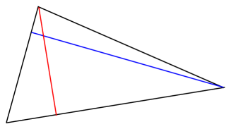
Figure 2. The triangle $\triangle\,\xi_{\nu}\xi_{\nu^{*}_{a}}\xi_{\nu^{**}_{a}}$

For case 2, we may assume $|\xi_{\nu^{*}_{a}}-\xi_{\nu^{**}_{a}}|<|\xi_{\nu}-\xi_{\nu^{*}_{a}}|\leq|\xi_{\nu}-\xi_{\nu^{**}_{a}}|$ by symmetry and denote $\triangle\,\xi_{\nu}\xi_{\nu^{*}_{a}}\xi_{\nu^{**}_{a}}$ as the triangle formed by $\xi_{\nu}$, $\xi_{\nu^{*}_{a}}$ and $\xi_{\nu^{**}_{a}}$ (Figure 2), with

$$H=\text{dist}\bigl{(}\xi_{\nu},\,\ell(\nu^{*}_{a},\nu^{**}_{a})\bigr{)},$$

$$h=\text{dist}\bigl{(}\xi_{\nu^{*}_{a}},\,\ell(\nu,\nu^{**}_{a})\bigr{)}.$$

Considering the measure of $\triangle\,\xi_{\nu}\xi_{\nu^{*}_{a}}\xi_{\nu^{**}_{a}}$, we get from (42)

$$h=\frac{|\xi_{\nu^{*}_{a}}-\xi_{\nu^{**}_{a}}|}{|\xi_{\nu^{**}_{a}}-\xi_{\nu}|}H\geq\frac{4}{K_{1}}\cdot\frac{10^{3}K_{1}}{K}\alpha 2^{\alpha}\cdot\frac{1}{4}>10^{3}\frac{\alpha 2^{\alpha}}{K},$$

where we have used $|\xi_{\nu^{**}_{a}}-\xi_{\nu}|\leq 4$ and hence (40) follows.

$\bullet$ An auxiliary lemma.

The the following lemma, which we are ready to prove, exhibits once more the spirit of Bourgain-Guth’s method, namely the failure of non-coplanar interactions implies small Fourier supports with possible addition separateness structures.

Lemma 5.1.

Let $B(0,R)\times[0,R]\subset\cup_{a}Q_{a}$ be as before. We have on each $Q_{a}$

$$|Tf(x)|\lesssim K^{8}\max_{\begin{subarray}{c}\nu_{1},\,\nu_{2},\,\nu_{2}\\ \text{non-collinear}\end{subarray}}\Bigl{(}\prod^{3}_{j=1}|T_{\nu_{j}}f|\Bigr{)}^{1/3}(x)$$ (45)

$$+\max_{\mu}\Bigl{|}\int_{\tilde{\Omega}_{\mu}}e^{i\phi(x,\xi)}\hat{f}(\xi)d\xi\Bigr{|}$$ (46)

$$+K^{2}_{1}\max_{\begin{subarray}{c}\mathcal{L}_{1},\mathcal{L}_{2}\subset\mathcal{L}_{a}\\ \text{dist}(\mathcal{L}_{1},\mathcal{L}_{2})>1/K_{1}\end{subarray}}\prod^{2}_{j=1}\Bigl{|}\sum_{\Omega_{\nu}\subset\mathcal{L}_{j}}e^{i\phi(x,\xi_{\nu})}T_{\nu}f\Bigr{|}^{\frac{1}{2}}(x)$$ (47)

$$+K^{3}_{1}K^{-\frac{1}{2}}\bigl{(}\sum_{\Omega_{\nu}\subset\mathcal{L}_{a}}|T_{\nu}f(x)|^{2}\bigr{)}^{\frac{1}{2}},$$ (48)

where $\tilde{\Omega}_{\mu}$ is a $\frac{1}{K_{1}}\times\frac{1}{K_{1}}$ square centered at $\xi_{\mu}\in\mathcal{I}$. $\mathcal{L}_{a}$ is a $(\alpha 2^{\alpha}10^{3}K_{1}/K)$-neighborhood of the line $\ell(\nu^{*}_{a},\nu^{**}_{a}):=\ell^{*}_{a}$. The two separated portions $\mathcal{L}_{1},\,\mathcal{L}_{2}$ of $\mathcal{L}_{a}$ are obtained by intersecting $\mathcal{L}_{a}$ with some $\tilde{\Omega}_{\mu_{1}}$ and $\tilde{\Omega}_{\mu_{2}}$ respectively.

Proof.

For $x\in Q_{a}$, we estimate $|Tf(x)|$ in different ways according to $a\in\mathcal{A}_{1}$, $a\in\mathcal{A}_{2}$ and $a\in\mathcal{A}_{3}$. If $a\in\mathcal{A}_{1}$, we have from the definition of $\mathcal{A}_{1}$

$$|Tf(x)|^{3} \leq(K^{2}c^{*}_{a})^{3}\leq K^{6}K^{12}c_{a,\,\nu_{1}}c_{a,\,\nu_{2}}c_{a,\,\nu_{3}}$$

$$\leq K^{18}\sum_{\begin{subarray}{c}\nu_{1},\,\nu_{2},\,\nu_{3}\\ \text{non-collinear}\end{subarray}}\prod^{3}_{j=1}|T_{\nu_{j}}f|(x)$$

$$\leq K^{24}\max_{\begin{subarray}{c}\nu_{1},\,\nu_{2},\,\nu_{3}\\ \text{non-collinear}\end{subarray}}\prod^{3}_{j=1}|T_{\nu_{j}}f|(x).$$

If $a\in\mathcal{A}_{2}$, we use the statement (41) for $\mathcal{A}_{2}$ to estimate $Tf(x)$. For brevity, we define $\|\xi\|=\max\{|\xi_{1}|,\,|\xi_{2}|\},\forall\xi\in\mathbb{R}^{2}$ and let

$$\Omega_{*}=\bigcup\Bigl{\{}\Omega_{\nu}\,\Big{|}\,\|\xi_{\nu}-\xi_{\nu^{*}_{a}}\|\leq 10/K_{1}\Bigr{\}}.$$

Then $\Omega_{*}$ is a $\frac{10}{K_{1}}\times\frac{10}{K_{1}}-$square with center $\xi_{\nu^{*}_{a}}$. We may write

$$|Tf(x)| \leq\Big{|}\sum_{\|\xi_{\nu}-\xi_{\nu^{*}_{a}}\|\leq 10/K_{1}}e^{i\phi(x,\,\xi_{\nu})}T_{\nu}f(x)\Bigr{|}+\Bigl{|}\sum_{\|\xi_{\nu}-\xi_{\nu^{*}_{a}}\|>10/K_{1}}e^{i\phi(x,\,\xi_{\nu})}T_{\nu}f(x)\Big{|}$$

$$\leq\Big{|}\sum_{\|\xi_{\nu}-\xi_{\nu^{*}_{a}}\|\leq 10/K_{1}}\int_{\Omega_{\nu}}e^{i\phi(x,\xi)}\hat{f}(\xi)d\xi\Big{|}+\sum_{|\xi_{\nu}-\xi_{\nu^{*}_{a}}|>4/K_{1}}\Big{|}T_{\nu}f(x)\Big{|}$$

$$\leq 100\max_{\tilde{\Omega}_{\mu}\subset\Omega_{\nu^{*}_{a}}}\Big{|}\int_{\tilde{\Omega}_{\mu}}e^{i\phi(x,\xi)}\hat{f}(\xi)d\xi\Big{|}+K^{2}K^{-4}c^{*}_{a}$$

$$\lesssim\eqref{3.2}+\eqref{3.3}.$$

If $a\in\mathcal{A}_{3}$, we write

$$Tf(x)=\mathfrak{D}_{1}+\mathfrak{D}_{2},$$

where

$$\mathfrak{D}_{j}=\chi_{a}(x)\int_{D_{j}}e^{i\phi(x,\xi)}\widehat{f}(\xi)d\xi,\,j=1,2,$$

with

$$D_{1}=\bigl{\{}\xi\,\mid\,\text{dist}(\xi,\ell^{*}_{a})>\alpha 2^{\alpha}10^{4}K_{1}/K\bigr{\}},\;D_{2}=\bigl{\{}\xi\,\mid\,\text{dist}(\xi,\ell^{*}_{a})\leq\alpha 2^{\alpha}10^{4}K_{1}/K\bigr{\}}.$$

From (43), we have

$$|\mathfrak{D}_{1}| \lesssim\sum_{\xi_{\nu}:\text{dist}(\xi_{\nu},\ell^{*}_{a})>\alpha 2^{\alpha}10^{3}K_{1}/K}\bigl{|}e^{i\phi(x,\xi_{\nu})}T_{\nu}f(x)\bigr{|}\leq K^{2}K^{-4}c^{*}_{a}\leq\eqref{3.3}.$$

To evaluate $\mathfrak{D}_{2}$, we assume without loss of generality

$$\text{supp}\,\widehat{f}\subset\Bigl{\{}\xi\in\mathbb{R}^{2}\;\Big{|}\;\text{dist}(\xi,\,\ell^{*}_{a})\leq\alpha 2^{\alpha}10^{4}\frac{K_{1}}{K}\Bigr{\}}.$$

Let $\{\tilde{\Omega}_{\mu}\}_{\mu}$ be a family of disjoint $\frac{1}{K_{1}}\times\frac{1}{K_{1}}-$squares such that $\mathcal{I}\subset\cup_{\mu}\tilde{\Omega}_{\mu}$. For any $x\in Q_{a}$, we define

$$c_{\mu}(x)=\int_{\tilde{\Omega}_{\mu}}e^{i\phi(x,\xi)}\hat{f}(\xi)d\xi.$$

Let

$$\mathcal{H}_{a}\mathrel{\mathop{=}^{\rm def}}\Bigl{\{}x\in Q_{a}\;\Big{|}\;\bigl{|}Tf(x)\bigr{|}\leq 10^{8}\max_{\mu}\bigl{|}c_{\mu}(x)\bigr{|}\Bigr{\}}.$$

Then

$$|\mathfrak{D}_{2}|\leq|Tf(x)|\chi_{\mathcal{H}_{a}}(x)+|Tf(x)|\chi_{Q_{a}\setminus\mathcal{H}_{a}}(x),$$

where the first term is bounded by (46). To handle the second term, we observe that $x\in Q_{a}\setminus\mathcal{H}_{a}$ implies

$$|c_{\mu}(x)|\leq 10^{-8}|Tf(x)|,\quad\forall\mu.$$ (49)

Consider the following set

$$\mathcal{J}(x)=\biggl{\{}\mu\;\Big{|}\;\frac{10^{-1}}{K^{2}_{1}}|Tf(x)|\leq|c_{\mu}(x)|\leq 10^{-8}|Tf(x)|,\,x\in Q_{a}\setminus\mathcal{H}_{a}\biggr{\}}.$$

We have $\#\mathcal{J}(x)\geq 10^{7},\forall\,x\in Q_{a}\setminus\mathcal{H}_{a}.$ Indeed, suppose$\#\mathcal{J}(x_{0})<10^{7}$ for some $x_{0}$, then

$$|Tf(x_{0})|\leq\sum_{\mu\in\mathcal{J}(x_{0})}|c_{\mu}(x_{0})|+\sum_{\mu\not\in\mathcal{J}(x_{0})}|c_{\mu}(x_{0})|.$$ (50)

Because of (49), we can bound the right side of (50) with

$$10^{7}\times 10^{-8}|Tf(x_{0})|+K^{2}_{1}\cdot\frac{10^{-1}}{K^{2}_{1}}|Tf(x_{0})|<\frac{1}{5}|Tf(x_{0})|,$$

which is impossible. Note that the centers of $\{\tilde{\Omega}_{\mu}\}_{\mu}$ are $\frac{1}{K_{1}}-$separated, we can choose $\mu_{1},\,\mu_{2}\in\mathcal{J}(x)$ ( $x-$dependent) such that

$$\text{dist}(\tilde{\Omega}_{\mu_{1}},\,\tilde{\Omega}_{\mu_{2}})\geq 10^{4}/K_{1},$$

and

$$|Tf(x)|\leq 10K^{2}_{1}\min\bigl{\{}|c_{\mu_{1}}(x)|,\,|c_{\mu_{2}}(x)|\bigr{\}},x\in Q_{a}\setminus\mathcal{H}_{a}.$$

It follows that

$$|Tf(x)|\chi_{Q_{a}\setminus\mathcal{H}_{a}}(x)\leq 10K^{2}_{1}\prod^{2}_{j=1}\Bigl{|}\int_{\tilde{\Omega}_{\mu_{j}}}e^{i\phi(x,\xi)}\widehat{f}(\xi)d\xi\Bigr{|}^{\frac{1}{2}},$$ (51)

where $\mu_{1}$ and $\mu_{2}$ might depend on $x$. Now in view of (41), we estimate further

$$|c_{\mu_{j}}(x)|\leq\Bigl{|}\sum_{\begin{subarray}{c}\Omega_{\nu}\subset\tilde{\Omega}_{\mu_{j}}\\ \text{dist}(\xi_{\nu},\ell^{*}_{a})\leq\alpha 2^{\alpha}10^{3}K_{1}/K\end{subarray}}\int_{\Omega_{\nu}}e^{i\phi(x,\xi)}\widehat{f}(\xi)d\xi\Bigr{|}+K^{2}\cdot K^{-4}c^{*}_{a}.$$ (52)

Thus

$$|Tf(x)|\chi_{Q_{a}\setminus\mathcal{H}_{a}}(x)$$

$$\leq 10K^{2}_{1}\Bigl{[}\prod^{2}_{j=1}\Bigl{|}\sum_{\Omega_{\nu}\subset\mathcal{L}_{j}}e^{i\phi(x,\xi_{\nu})}T_{\nu}f\Bigr{|}^{\frac{1}{2}}(x)+\Bigl{(}2K^{-2}c^{*}_{a}\sum_{\Omega_{\nu}\subset\mathcal{L}_{a}}|T_{\nu}f(x)|\Bigr{)}^{\frac{1}{2}}+K^{-2}c^{*}_{a}\Bigr{]},$$ (53)

where $\mathcal{L}_{j}=\tilde{\Omega}_{\mu_{j}}\cap\mathcal{L}_{a}$, with $\mathcal{L}_{a}$ an $\alpha 2^{\alpha}10^{3}K_{1}/K-$neighborhood of $\ell^{*}_{a}$. Note that

$$c^{*}_{a}\leq\bigl{(}\sum_{\Omega_{\nu}\subset\mathcal{L}_{a}}|T_{\nu}f(x)|^{2}\bigr{)}^{\frac{1}{2}},$$

and

$$\sum_{\Omega_{\nu}\subset\mathcal{L}}|T_{\nu}f(x)|\lesssim_{\alpha}K_{1}K^{\frac{1}{2}}\bigl{(}\sum_{\Omega_{\nu}\subset\mathcal{L}_{a}}|T_{\nu}f(x)|^{2}\bigr{)}^{\frac{1}{2}},$$

the last two terms in (53) is bounded by

$$K^{3}_{1}K^{-\frac{1}{2}}\bigl{(}\sum_{\Omega_{\nu}\subset\mathcal{L}_{a}}|T_{\nu}f(x)|^{2}\bigr{)}^{\frac{1}{2}}.$$

Therefore, we have

$$|\mathfrak{D}_{2}|\lesssim\eqref{3.2}+\eqref{3.1}+\eqref{3.3}.$$

This completes the proof of Lemma 5.1. ∎

5.2. A self-similar iterative formula

The formula we deduce in this part is the engine for the iterating process in order for the fractional order Bourgain-Guth’s inequality. Let $\Omega_{\tau}$ be a $\delta-$square centered at $\xi_{\tau}$,

$$\Omega^{\tau}_{\nu}\mathrel{\mathop{=}^{\rm def}}\Bigl{\{}\xi\in\mathbb{R}^{2}\,\Big{|}\,\|\xi-(\xi_{\tau}+\delta\xi_{\nu})\|<\frac{\delta}{K}\Bigr{\}},\;$$

$$\tilde{\Omega}^{\tau}_{\mu}\mathrel{\mathop{=}^{\rm def}}\Bigl{\{}\xi\in\mathbb{R}^{2}\,\Big{|}\,\|\xi-(\xi_{\tau}+\delta\xi_{\mu})\|<\frac{\delta}{K_{1}}\Bigr{\}}.$$

Denote by $\widehat{f}_{\tau,\nu}=\widehat{f}\cdot\chi_{\Omega^{\tau}_{\nu}}$. We prove the following iterative formula from scale $\delta$ to $\frac{\delta}{K}$ for all $a\in\mathcal{A}$

$$|T_{\tau}f|(x)\lesssim K^{8}\max_{\begin{subarray}{c}\nu_{1},\,\nu_{2},\,\nu_{3}\\ \text{non-collinear}\end{subarray}}\prod^{3}_{j=1}\left|Tf_{\tau,\,\nu_{j}}\right|^{\frac{1}{3}}(x)$$ (54)

$$+\psi_{\tau}(x)\Big{(}\sum_{\Omega^{\tau}_{\nu}\subset\mathcal{L}_{\tau}}|Tf_{\tau,\,\nu}|^{2}\Big{)}^{\frac{1}{2}}(x)$$ (55)

$$+\max_{\mu}\Bigl{|}\int_{\tilde{\Omega}^{\tau}_{\mu}\cap\Omega_{\tau}}e^{i[\xi\cdot x^{\prime}+x_{3}|\xi|^{\alpha}]}\hat{f}(\xi)d\xi\Bigr{|},$$ (56)

for all $x\in\mathcal{T}^{*}_{a}$, where

$$\mathcal{T}^{*}_{a}\mathrel{\mathop{=}^{\rm def}}\Bigl{\{}x\in\mathbb{R}^{3}\,\Big{|}\,|x_{1}-a_{1}|<\frac{K}{\delta},\,|x_{2}-a_{2}|<\frac{K}{\delta},\,|x_{3}-a_{3}|<\frac{K}{\delta^{\alpha}}\Bigr{\}},$$

and $\mathcal{L}_{\tau}$ is a $\delta/K-$neighborhood of a line segment. $\psi_{\tau}$ is a function satisfying

$$\left(\frac{1}{|B|}\int_{B}\psi_{\tau}^{4}(x)dx\right)^{1/4}\lesssim K^{2\alpha}_{1},$$ (57)

where $B$ is a $K\mathcal{C}^{*}_{\tau}-$box centered at $a$.

To deduce (54)-(57), we need the following estimate, which is standard square functions going back to Cordoba [Co]. The crucial $L^{4}$-estimate is used in [BG] to tackle the worst scenario by exploiting the separateness of the line segments in which the frequencies locate. This part of frequencies corresponds to the terms of main contributions.

Lemma 5.2.

For any $a\in\mathcal{A}$ and all $x\in Q_{a}$, we have

$$\Bigl{(}\frac{1}{|Q_{a}|}\int_{Q_{a}}\bigl{|}\eqref{3.1}+\eqref{3.3}\bigr{|}^{4}dx\Bigr{)}^{1/4}\lesssim K^{2\alpha}_{1}\Bigl{(}\sum_{\Omega_{\nu}\subset\mathcal{L}}|T_{\nu}f(x)|^{2}\Bigr{)}^{\frac{1}{2}},$$ (58)

where the implicit constant is independent of $a$.

Remark 15.

This observation is crucial for the iteration in the next subsection. To prove (58), we rely heavily on the $10^{4}/K_{1}-$separateness of the segments $\mathcal{L}_{1},\,\mathcal{L}_{2}$. Since we are dealing with the fractional order symbol, the proof is more intricate than that in [BG], where the algebraic structure simplifies the proof significantly.

Proof.

We need to estimate the $L^{4}-$averagement of (47) and (48) over $Q_{a}$. Since on every $Q_{a}$, $|T_{\nu}f(x)|$ can be viewed as a constant, we immediately get

$$\Bigl{(}\frac{1}{|Q_{a}|}\int_{Q_{a}}\eqref{3.3}^{4}dx\Bigr{)}^{\frac{1}{4}}\lesssim K^{3}_{1}\Bigl{(}\sum_{\Omega_{\nu}\subset\mathcal{L}}|T_{\nu}f(x)|^{2}\Bigr{)}^{\frac{1}{2}}.$$

Next, we estimate (47). First, we have

$$\int_{Q_{a}}\max_{\begin{subarray}{c}\mathcal{L}_{1},\mathcal{L}_{2}\subset\mathcal{L}_{a}\\ \text{dist}(\mathcal{L}_{1},\mathcal{L}_{2})\geq\frac{10^{4}}{K_{1}}\end{subarray}}\prod^{2}_{j=1}\Bigl{|}\sum_{\Omega_{\nu}\subset\mathcal{L}_{j}}e^{i\phi(x,\xi_{\nu})}T_{\nu}f(x)\Bigr{|}^{2}(x)dx$$

$$\leq \sum_{\begin{subarray}{c}\mathcal{L}_{1},\mathcal{L}_{2}\subset\mathcal{L}_{a}\\ \text{dist}(\mathcal{L}_{1},\mathcal{L}_{2})\geq\frac{10^{4}}{K_{1}}\end{subarray}}\int_{Q_{a}\cap\mathfrak{S}_{\mathcal{L}_{1},\mathcal{L}_{2}}}\prod^{2}_{j=1}\Bigl{|}\sum_{\Omega_{\nu}\subset\mathcal{L}_{j}}e^{i\phi(x,\xi_{\nu})}T_{\nu}f(x)\Bigr{|}^{2}(x)dx$$ (59)

where

$$\mathfrak{S}_{\mathcal{L}_{1},\,\mathcal{L}_{2}}\mathrel{\mathop{=}^{\rm def}}\biggl{\{}x\,\Big{|}\;\eqref{3.1}\leq 2\,\Bigl{|}\sum_{\Omega_{\nu}\subset\mathcal{L}_{1}}e^{i\phi(x,\xi_{\nu})}T_{\nu}f\Bigr{|}^{\frac{1}{2}}\Bigl{|}\sum_{\Omega_{\nu}\subset\mathcal{L}_{2}}e^{i\phi(x,\xi_{\nu})}T_{\nu}f\Bigr{|}^{\frac{1}{2}}(x)\biggr{\}},$$

and the summation in (59) is taken over all the pairs of $10^{4}/K_{1}-$separated subsegments of $\mathcal{L}_{a}$. Since there are at most $K^{2}_{1}$ pairs of such subsegments, it suffices to estimate each term in the summation. Take a Schwartz function $\rho\geq 0$ such that $\widehat{\rho}$ is compactly supported and $\rho_{a}(x):=\rho\big{(}\frac{x-a}{K}\big{)}=1$ for all $x\in Q_{a}$

$$\int_{Q_{a}\cap\mathfrak{S}_{\mathcal{L}_{1},\,\mathcal{L}_{2}}}\prod^{2}_{j=1}\Bigl{|}\sum_{\Omega_{\nu}\subset\mathcal{L}_{j}}e^{i\phi(x,\xi_{\nu})}T_{\nu}f(x)\Bigr{|}^{2}dx$$ (60)

$$\leq \int_{\mathbb{R}^{3}}\prod^{2}_{j=1}\Bigl{|}\rho_{a}(x)\sum_{\Omega_{\nu}\subset\mathcal{L}_{j}}e^{i\phi(x,\xi_{\nu})}T_{\nu}f(x)\Bigr{|}^{2}dx$$ (61)

$$\leq \sum_{\begin{subarray}{c}\Omega_{\nu_{1}},\,\Omega_{\nu_{2}}\subset\mathcal{L}_{1}\\ \Omega_{\nu^{\prime}_{1}},\,\Omega_{\nu^{\prime}_{2}}\subset\mathcal{L}_{2}\end{subarray}}\Bigl{|}\int_{\mathbb{R}^{3}}\big{[}\rho_{a}T_{\nu_{1}}f\cdot\overline{\rho_{a}T_{\nu_{2}}f\cdot\rho_{a}T_{\nu^{\prime}_{1}}f}\cdot\rho_{a}T_{\nu^{\prime}_{2}}f\big{]}(x)e^{i\Psi(x,\,\xi_{\nu_{1}},\,\xi_{\nu_{2}},\,\xi_{\nu^{\prime}_{1}},\,\xi_{\nu^{\prime}_{2}})}dx\Bigr{|},$$

where

$$\Psi(x,\,\xi_{\nu_{1}},\,\xi_{\nu_{2}},\,\xi_{\nu^{\prime}_{1}},\,\xi_{\nu^{\prime}_{2}})=\phi(x,\xi_{\nu_{1}})-\phi(x,\xi_{\nu_{2}})-\phi(x,\xi_{\nu^{\prime}_{1}})+\phi(x,\xi_{\nu^{\prime}_{2}}).$$

Considering the support of the function

$$\widehat{\rho_{a}}*\widehat{T_{\nu_{1}}f}*\widehat{\rho_{a}}*\widehat{\overline{T_{\nu_{2}}f}}*\widehat{\rho_{a}}*\widehat{\overline{T_{\nu^{\prime}_{1}}f}}*\widehat{\rho_{a}}*\widehat{T_{\nu^{\prime}_{2}}f},$$

we may restrict the summation to those quadruples $\nu_{1},\,\nu_{2},\,\nu^{\prime}_{1},\,\nu^{\prime}_{2}$ such that

$$\begin{cases}|\xi_{\nu_{1}}-\xi_{\nu_{2}}-\xi_{\nu^{\prime}_{1}}+\xi_{\nu^{\prime}_{2}}|\lesssim\frac{1}{K},\\ \big{|}|\xi_{\nu_{1}}|^{\alpha}-|\xi_{\nu_{2}}|^{\alpha}-|\xi_{\nu^{\prime}_{1}}|^{\alpha}+|\xi_{\nu^{\prime}_{2}}|^{\alpha}\big{|}\lesssim\frac{1}{K}.\end{cases}$$ (62)

Denote by $\ell^{*}_{a}=\mathbb{R}v+b$ where $v,\,b\in\mathbb{R}^{2}$ with $|v|=1$, $|b|\leq 4$ and $v\perp b$. Since $\xi_{\nu_{1}},\,\xi_{\nu_{2}},\,\xi_{\nu^{\prime}_{1}}$ and $\xi_{\nu^{\prime}_{2}}$ are lying in a $\frac{\alpha 2^{\alpha}10^{3}K_{1}}{K}-$ neighborhood of $\ell^{*}_{a}$, there are $t_{1},\,t_{2},\,t^{\prime}_{1}$ and $t^{\prime}_{2}$ such that for $j=1,2$, we have

$$|\xi_{\nu_{j}}-t_{j}v-b|\leq\alpha 2^{\alpha}10^{3}\frac{K_{1}}{K},\;|\xi_{\nu^{\prime}_{j}}-(t^{\prime}_{j})v-b|\leq\alpha 2^{\alpha}10^{3}\frac{K_{1}}{K}.$$

In view of (62) and the $10^{4}/K_{1}-$separateness of $\mathcal{L}_{1}$ and $\mathcal{L}_{2}$, we have

$$|t_{1}-t_{2}|<\frac{2}{K_{1}},\,|t^{\prime}_{1}-t^{\prime}_{2}|<\frac{2}{K_{1}},\;|t_{1}-t^{\prime}_{1}|>\frac{10^{4}}{K_{1}},$$ (63)

$$|t_{1}-t_{2}-t^{\prime}_{1}+t^{\prime}_{2}|\lesssim\frac{K_{1}}{K},$$ (64)

$$|\varphi(t_{1})-\varphi(t_{2})-\varphi(t^{\prime}_{1})+\varphi(t^{\prime}_{2})|\lesssim\frac{K_{1}}{K},$$ (65)

where $\varphi(t):=(t^{2}+|b|^{2})^{\frac{\alpha}{2}}$. We claim (63), (64) and (65) imply

$$|t_{1}-t_{2}|\lesssim\frac{K^{\alpha}_{1}}{K},\quad|t^{\prime}_{1}-t^{\prime}_{2}|\lesssim\frac{K^{\alpha}_{1}}{K}.$$ (66)

As a consequence, we may deduce that

$$|\xi_{\nu_{1}}-\xi_{\nu_{2}}|\lesssim\frac{K^{\alpha}_{1}}{K},\,|\xi_{\nu^{\prime}_{1}}-\xi_{\nu^{\prime}_{2}}|\lesssim\frac{K^{\alpha}_{1}}{K},$$

which implies

$$\eqref{bilinear1}\lesssim K^{4\alpha}_{1}\sum_{\Omega_{\nu}\subset\mathcal{L}_{1},\,\Omega_{\nu^{\prime}}\subset\mathcal{L}_{2}}\int_{Q_{a}}|Tf_{\nu}|^{2}|Tf_{\nu^{\prime}}|^{2}(x)dx.$$

Summing up (60) with respect to pairs of $(\mathcal{L}_{1},\,\mathcal{L}_{2})$, we obtain from the local constant property fulfilled by the $|T_{\nu}f|(x)$’s

$$\int_{Q_{a}}|\eqref{3.1}|^{4}dx\lesssim K^{4\alpha+2}_{1}\int_{Q_{a}}\Bigl{(}\sum_{\Omega_{\nu}\subset\mathcal{L}}|Tf_{\nu}(x)|^{2}\Bigr{)}^{2}dx$$

$$\lesssim K^{4\alpha+2}_{1}|Q_{a}|\Bigl{(}\sum_{\Omega_{\nu}\subset\mathcal{L}}|Tf_{\nu}(x)|^{2}\Bigr{)}^{2},\quad\forall\,x\in Q_{a}.$$

This proves (58).

To prove the claim (66), we need to consider the following two possibilities.

$$t_{1}<t_{2}<t^{\prime}_{1}<t^{\prime}_{2}\,,\;\text{and}\quad t_{1}<t_{2}<t^{\prime}_{2}<t^{\prime}_{1}.$$

In view of (64), the second possibility implies

$$|t_{1}-t_{2}|+|t^{\prime}_{1}-t^{\prime}_{2}|\lesssim\frac{K_{1}}{K}.$$

Then (66) follows immediately. It is thus sufficient to handle the first possibility. To do this, we consider the following three cases. $\bullet$ $t_{1}<t_{2}<0<t^{\prime}_{1}<t^{\prime}_{2}$. For this case, we have from (65)

$$\bigl{|}\varphi(t_{1})-\varphi(t_{2})\bigr{|}+\bigl{|}\varphi(t^{\prime}_{1})-\varphi(t^{\prime}_{2})\bigr{|}\lesssim\frac{K_{1}}{K}.$$ (67)

By triangle inequality and (63), we have either $t^{\prime}_{1}>\frac{10^{3}}{K_{1}}$ or $t_{2}<-\frac{10^{3}}{K_{1}}$. We only handle the case when $t^{\prime}_{1}>\frac{10^{3}}{K_{1}}$ since the other one is exactly the same. We apply mean value theorem to $\varphi(t)$ to get a $t_{*}$ with $t^{\prime}_{1}<t_{*}<t^{\prime}_{2}$ such that

$$\frac{K_{1}}{K}\gtrsim\bigl{|}\varphi(t^{\prime}_{1})-\varphi(t^{\prime}_{2})\bigr{|}\gtrsim\alpha|t_{*}|^{\alpha-1}|t^{\prime}_{1}-t^{\prime}_{2}|\gtrsim\frac{\alpha}{K^{\alpha-1}_{1}}|t^{\prime}_{1}-t^{\prime}_{2}|.$$

Hence, we have

$$|t^{\prime}_{1}-t^{\prime}_{2}|\lesssim_{\alpha}\frac{K^{\alpha}_{1}}{K}.$$

By triangle inequality again and (64), we obtain

$$|t_{1}-t_{2}|\lesssim_{\alpha}\frac{K^{\alpha}_{1}}{K}.$$

$\bullet$ $t_{1}<0<t_{2}<t^{\prime}_{1}<t^{\prime}_{2}$. First, we always have $t^{\prime}>\frac{10^{3}}{K_{1}}$ in this case. If $t_{1}<-t_{2}$, we also get (67), so (66) follows immediately as above. For $-t_{2}\leq t_{1}$, we have from (65)

$$\Bigl{|}\bigl{|}\varphi(t_{1})-\varphi(t_{2})\bigr{|}-\bigl{|}\varphi(t^{\prime}_{1})-\varphi(t^{\prime}_{2})\bigr{|}\Bigr{|}\lesssim\frac{K_{1}}{K}.$$ (68)

Suppose $|t_{1}-t_{2}|\gg\frac{K^{\alpha}_{1}}{K}$, then $|t^{\prime}_{1}-t^{\prime}_{2}|\gg\frac{K^{\alpha}_{1}}{K}$ by (63). Moreover, we have

$$\frac{1}{2}|t^{\prime}_{1}-t^{\prime}_{2}|\leq|t_{1}-t_{2}|\leq 2|t^{\prime}_{1}-t^{\prime}_{2}|.$$ (69)

By mean value theorem, we have for some $t_{*}\in(t_{1},t_{2})$, $t^{\prime}_{*}\in(t^{\prime}_{1},t^{\prime}_{2})$ with $t^{\prime}_{*}>\max\{\frac{10^{3}}{K_{1}},\,t_{*}+\frac{10^{3}}{K_{1}}\}$ such that

$$\frac{K_{1}}{K} \gtrsim\Bigl{|}\bigl{(}\varphi(t^{\prime}_{2})-\varphi(t^{\prime}_{1})\bigr{)}-\bigl{(}\varphi(t_{2})-\varphi(t_{1})\bigr{)}\Bigr{|}$$

$$\gg\alpha\frac{K^{\alpha}_{1}}{K}\Big{(}|t^{\prime}_{*}|^{\alpha-1}-|t_{*}|^{\alpha-1}\Big{)}\gg\alpha\frac{K_{1}}{K},$$

which is impossible since $\alpha>1$ and $K_{1}\gg 1$.

$\bullet$ $0<t_{1}<t_{2}<t^{\prime}_{1}<t^{\prime}_{2}$. This can be reduced to the above two cases, and we complete the proof of (58). ∎

Here, another observation made by Bourgain and Guth in [BG] is that as a consequence of (58), for $x\in Q_{a}$ one define $\psi(x)$ by writing

$$\eqref{3.1}+\eqref{3.3}=\psi(x)\Bigl{(}\sum_{\Omega_{\nu}\subset\mathcal{L}}|Tf_{\nu}(x)|^{2}\Bigr{)}^{\frac{1}{2}}.$$

Clearly $\psi$ is nonnegative such that

$$\Bigl{(}\frac{1}{|Q_{a}|}\int_{Q_{a}}\psi^{4}(x)dx\Bigr{)}^{1/4}\lesssim K^{2\alpha}_{1}.$$ (70)

To see this is possible, one only need to be aware of the local constant property enjoyed by $T_{\nu}f(x)$’s so that $\psi(x)$ can be defined on each ball of radius $K$ due to (58). Then we glue all the pieces of $\psi(x)$ on the balls together. By an average argument and the local constancy property of $\eqref{3.1}+\eqref{3.3}$ and functions $T_{\nu}f(x)$ on each $Q_{a,K}$ box, we may assume $\psi(x)$ is constant on the unit cubes centered at lattices.

Remark 16.

By writing (47) + (48) into a product of an appropriate $\psi$ and a square function, we may iterate this part step by step in the subsequent context to generate the items having transverality structures corresponding to all the dyadic scales. This is one of the brilliant ideas due to Bourgain and Guth, which is also applied by Bourgain in [B3] and [BG] as a substitution of Wolff’s induction on scale technique.

Substituting $\eqref{3.1}+\eqref{3.3}$ in Lemma 5.1 for

$$\psi(x)\Bigl{(}\sum_{\Omega_{\nu}\subset\mathcal{L}}|Tf_{\nu}(x)|^{2}\Bigr{)}^{\frac{1}{2}},$$

we obtain

$$|Tf(x)|\lesssim K^{8}\max_{\begin{subarray}{c}\nu_{1},\,\nu_{2},\,\nu_{2}\\ \text{non-collinear}\end{subarray}}\Bigl{(}\prod^{3}_{j=1}|T_{\nu_{j}}f|\Bigr{)}^{1/3}(x)$$ (71)

$$+\psi(x)\Bigl{(}\sum_{\Omega_{\nu}\subset\mathcal{L}}|Tf_{\nu}(x)|^{2}\Bigr{)}^{\frac{1}{2}}$$ (72)

$$+\max_{\mu}\Bigl{|}\int_{\tilde{\Omega}_{\mu}}e^{i\phi(x,\xi)}\hat{f}(\xi)d\xi\Bigr{|}.$$ (73)

Now, we are ready to prove (54)-(57). Observe that $Tf(x)$ is controlled in terms of $Tf_{\nu}$’s with $\widehat{f}_{\nu}$ supported in a square of size $\frac{1}{K}$, whereas $\widehat{f}$ is supported in a region of size $1$. Thus it is natural to scale each $\widehat{f}_{\nu}$ to be a function $\widehat{g}_{\nu}$ such that supp $\widehat{g}_{\nu}$ is of size $1$. After applying (71)-(73) to each $Tg_{\nu}$, we rescale the estimates on $Tg_{\nu}$ back to the original size $\frac{1}{K}$. More generally, this process can be carried out with $Tf_{\tau}$ in place of $Tf(x)$ on the left side of (71), where $\widehat{f}_{\tau}$ is supported in a square of size $\delta$.

Proof of (54)-(57).

Let $\widehat{f}_{\tau}=\widehat{f}|_{\Omega_{\tau}}$ and $x\in\mathcal{T}^{*}_{a}=a+Q^{\delta}_{0,K},$ with

$$Q^{\delta}_{0,K}=\{x\,\mid\,(\delta x_{1},\delta x_{2},\delta^{\alpha}x_{3})\in Q_{0,K}\}.$$

Making change of variables

$$x^{\prime}=a^{\prime}+\tilde{x}^{\prime}/\delta,\;x_{3}=a_{3}+\tilde{x}_{3}/\delta^{\alpha},\;\xi=\xi_{\tau}+\delta\eta,$$ (74)

where $\xi_{\tau}$ the center of $\Omega_{\tau}$, and $\tilde{x}\in Q_{0,K}$, we have

$$\chi_{\mathcal{T}^{*}_{a}}(x)Tf_{\tau}(x)= \chi_{Q_{0,K}}(\tilde{x})\int_{\Omega}e^{i[\tilde{x}^{\prime}\cdot\eta+\tilde{x}_{3}|\eta|^{\alpha}]}\widehat{g^{\tau,\delta}_{a}}(\eta)d\eta$$

$$= \chi_{Q_{0,K}}(\tilde{x})T(g^{\tau,\delta}_{a})(\tilde{x}),$$ (75)

with

$$\widehat{g^{\tau,\delta}_{a}}(\eta)=e^{i[\delta a^{\prime}\cdot\eta+a_{3}\delta^{\alpha}|\eta|^{\alpha}+(a^{\prime}+\tilde{x}^{\prime}/\delta)\cdot\xi_{\tau}+(a_{3}+\tilde{x}_{3}/\delta^{\alpha})(|\xi_{\tau}+\delta\eta|^{\alpha}-|\delta\eta|^{\alpha})]}\delta^{2}\widehat{f}_{\tau}(\xi_{\tau}+\delta\eta)\chi_{\Omega}(\eta).$$

Now that $\widehat{g^{\tau,\delta}_{a}}$ is supported in a square of size $1$, we can apply (71)-(73) to (75) with $\tilde{x}\in Q_{0,K}$ to obtain

$$\Bigl{|}T(g^{\tau,\delta}_{a})(\tilde{x})\Bigr{|}\lesssim K^{8}\max_{\begin{subarray}{c}\nu_{1},\nu_{2},\nu_{3}\\ \text{non-collinear}\end{subarray}}\prod^{3}_{j=1}\bigl{|}T_{\nu_{j}}(g^{\tau,\delta}_{a})\bigr{|}^{\frac{1}{3}}(\tilde{x})$$ (76)

$$+\psi(\tilde{x})\Bigl{(}\sum_{\Omega_{\nu}\subset\mathcal{L}}|T_{\nu}(g^{\tau,\delta}_{a})|^{2}\Bigr{)}^{\frac{1}{2}}(\tilde{x})$$ (77)

$$+\max_{\mu}\bigl{|}\int_{\widetilde{\Omega}_{\mu}}e^{i\phi(\tilde{x},\xi)}\widehat{g^{\tau,\delta}_{a}}(\eta)d\eta\bigr{|}.$$ (78)

Re-scale the $\widehat{g^{\tau,\delta}_{a}}$ in (76)-(78) back to $\widehat{f}_{\tau}$ by using (74) and setting $\eta=(\zeta-\xi_{\tau})/\delta$

$$\Bigl{|}\chi_{Q_{0,K}}(\tilde{x})T_{\nu}(g^{\tau,\delta}_{a})(\tilde{x})\Bigr{|} =\Bigl{|}\int_{\|\eta-\xi_{\nu}\|<1/K}e^{i[\tilde{x}^{\prime}\cdot\eta+\tilde{x}_{3}|\eta|^{\alpha}]}\widehat{g^{\tau,\delta}_{a}}(\eta)d\eta\Bigr{|}$$

$$=\Bigl{|}\int_{\|\zeta-(\xi_{\tau}+\delta\xi_{\nu})\|<\delta/K}e^{i[\zeta\cdot(a^{\prime}+\tilde{x}/\delta)+(a_{3}+\frac{\tilde{x}_{3}}{\delta^{\alpha}})|\zeta|^{\alpha}]}\hat{f}_{\tau}(\zeta)d\zeta\Bigr{|}$$

$$=\Bigl{|}\int_{\|\zeta-(\xi_{\tau}+\delta\xi_{\nu})\|<\delta/K}e^{i[\zeta\cdot x^{\prime}+x_{3}|\zeta|^{\alpha}]}\hat{f}_{\tau}(\zeta)d\zeta\Bigr{|},\;x\in\mathcal{T}^{*}_{a}.$$ (79)

From (75), (76) and (79), we get (54)-(56) on $\mathcal{T}^{*}_{a}$.

Since

$$\psi_{\tau}(x)=\psi\bigl{(}\delta(x_{1}-a_{1}),\,\delta(x_{2}-a_{2}),\,\delta^{\alpha}(x_{3}-a_{3})\bigr{)},\forall\;x\in\mathcal{T}^{*}_{a},$$

we obtain (57) from (70). ∎

5.3. Iteration and the end of the proof

This part follows intimately the idea of Bourgain and Guth in [BG] however, we provide more explicit calculations during the iteration process so that this marvelous idea can be reached even for the novice readers. It is hoped that this robust machine will be upgraded so that further improvements seems possible in this area.

Let $1\ll K_{1}\ll K\ll R$. From Lemma 5.1, we have

$$|Tf(x)|\lesssim \,K^{8}\max_{\begin{subarray}{c}\Omega_{\tau_{1}},\,\Omega_{\tau_{2}},\,\Omega_{\tau_{3}}:\frac{1}{K}-\text{cubes}\\ \text{non-collinear}\end{subarray}}\prod^{3}_{j=1}|T_{\tau_{j}}f|^{\frac{1}{3}}(x)$$ (80)

$$+\psi(x)\Big{[}\sum_{\begin{subarray}{c}\Omega_{\tau}\subset\mathcal{L}\\ \Omega_{\tau}:\frac{1}{K}-\text{cubes}\end{subarray}}|T_{\tau}f|^{2}\Big{]}^{1/2}(x)$$ (81)

$$+\max_{\tilde{\Omega}_{\tilde{\tau}}:\frac{1}{K_{1}}-\text{cubes}}|T_{\tilde{\tau}}f|(x),$$ (82)

where $\psi$ is approximately constants on unit boxes and obeys

$$\bigg{(}\frac{1}{|Q_{a}|}\int_{Q_{a}}\psi^{4}(x)dx\bigg{)}^{\frac{1}{4}}\lesssim K_{1}^{2\alpha},$$

for any $Q_{a}$.

Noting that (80) involves a triple product of $|T_{\tau_{j}}f|^{\frac{1}{3}}$ with $j=1,2,3$, we call this term is of type I. For (81), it is a product of a suitable function $\psi$ and an $\ell^{2}$ sum of $\{T_{\tau}f\}_{\tau}$, and we call this term is of type II. The term (82) is an $\ell^{\infty}$ norm of $\{T_{\widetilde{\tau}}f\}_{\widetilde{\tau}}$, and we call it of type III. In each step of the iteration below, we will encounter plenty of terms belonging to type I, II and III from the previous step. These are called newborn terms. We add the newborn terms of type I to the type I terms of the previous generations and keep on iterating all the newborn terms of type II and III to get the next generation of type I, II and III terms. This is the iterating mechanism.

To be more precise, we use (54) - (56) to $T_{\tau}f$ in (81) with $\delta=1/K$ and to $T_{\tilde{\tau}}f$ in (82), with $\delta=1/K_{1}$. This is exactly the first step of the iteration. After this, we obtain terms of type I, type II and type III generated by (81) and (82). In each type of the terms, the supports of $\widehat{f}_{\tau}$’s could be of the scales like

$$\frac{1}{K^{2}},\quad\frac{1}{KK_{1}}\quad\text{or}\quad\frac{1}{K^{2}_{1}}.$$

Adding the newborn terms of type I to the previous type I terms, we repeat the same argument as in the first step to all the terms of type II and type III to get the second generation. This process is continued with newborn terms of type I added to the pervious type I terms until the scale of the support of $\widehat{f}_{\tau}$ in the terms of type II and type III becomes $\frac{1}{\sqrt{R}}$. Finally, we obtain a collection of type I terms at different scales and a remainder consisting of type II and III terms at scale $\frac{1}{\sqrt{R}}$, which is controlled by (4). This yields (3) and (4).

Now, we present the explicit computation for the first step. Applying (54) - (56) to (81) with $\delta=1/K$, we have by Minkowski’s inequality

$$\quad\psi(x)\Bigl{(}\sum_{\Omega_{\tau}\subset\mathcal{L}}|T_{\tau}f|^{2}\Bigr{)}^{1/2}(x)$$

$$\lesssim K^{8}\Bigg{[}\sum_{\Omega_{\tau}\subset\mathcal{L}}\Bigg{(}\max_{\begin{subarray}{c}\Omega_{\tau}\supset\Omega_{\tau^{(1)}_{1}},\,\Omega_{\tau^{(1)}_{2}},\,\Omega_{\tau^{(1)}_{3}}(x)\\ \frac{1}{K^{2}}-\text{squares};\,\text{non-collinear}\end{subarray}}\psi\prod^{3}_{j=1}|T_{\tau^{(1)}_{j}}f|^{\frac{1}{3}}\Bigg{)}^{2}\Bigg{]}^{\frac{1}{2}}(x)$$ (83)

$$\quad+\Bigg{[}\sum_{\Omega_{\tau}\subset\mathcal{L}}\sum_{\begin{subarray}{c}\mathcal{L}^{(1)}\supset\Omega_{\tau^{(1)}}\\ \frac{1}{K^{2}}-\text{squares}\end{subarray}}\bigl{(}\psi\psi_{\tau}|T_{\tau^{(1)}}f|\bigr{)}^{2}\Bigg{]}^{\frac{1}{2}}(x)$$ (84)

$$\quad+\Bigg{(}\sum_{\Omega_{\tau}\subset\mathcal{L}}\psi^{2}\max_{\begin{subarray}{c}\tilde{\Omega}_{\tilde{\tau}^{(1)}}\subset\Omega_{\tau}\\ \frac{1}{K_{1}K}-\text{squares}\end{subarray}}|T_{\tilde{\tau}^{(1)}}f|^{2}\Bigg{)}^{\frac{1}{2}}(x),$$ (85)

where the superscript in $\tau^{(k)}$ denotes the $k-$th step of the iteration.

Denoting $\psi_{:\tau^{(1)}:}=\psi\psi_{\tau}$, we need to verify for any $\varepsilon>0$

$$\frac{1}{|\mathcal{C}^{*}_{\tau}|}\int_{\mathcal{C}^{*}_{\tau}}\psi^{4}(x)dx\lesssim R^{\varepsilon},$$ (86)

and

$$\frac{1}{|\mathcal{C}^{*}_{\tau^{(1)}}|}\int_{\mathcal{C}^{*}_{\tau^{(1)}}}\psi_{:\tau^{(1)}:}^{4}(x)dx\lesssim R^{\varepsilon}.$$ (87)

To get (86), we use the boxes $Q_{a}$ to subdivide $\mathcal{C}^{*}_{\tau}$ such that

$$\mathcal{C}^{*}_{\tau}\subset\bigcup_{a}{Q_{a}}\subset 2\mathcal{C}^{*}_{\tau}.$$

Then (70) gives

$$\frac{1}{|\mathcal{C}^{*}_{\tau}|}\int_{\mathcal{C}^{*}_{\tau}}\psi^{4}(x)dx \lesssim\frac{1}{|\bigcup_{a}Q_{a}|}\int_{\cup Q_{a}}\psi^{4}(x)dx$$

$$\lesssim\max_{\mathcal{C}^{*}_{\tau}\subset Q_{a}\subset 2\mathcal{C}^{*}_{\tau}}\frac{1}{|Q_{a}|}\int_{Q_{a}}\psi^{4}(x)dx\lesssim K^{8\alpha}_{1}\ll R^{\varepsilon}.$$

To verify (87), we note that $\mathcal{C}^{*}_{\tau^{(1)}}$ is a $K^{2}\times K^{2}\times K^{2\alpha}-$box in the direction of the normal vector of the surface at $\xi_{\tau^{(1)}}$. It follows that $\mathcal{C}^{*}_{\tau^{(1)}}$ can be covered as follows

$$\mathcal{C}^{*}_{\tau^{(1)}}\subset\bigcup_{\tau}B^{*}_{\tau}\subset 2\mathcal{C}^{*}_{\tau^{(1)}}$$

where $B^{*}_{\tau}$ is a $K\mathcal{C}^{*}_{\tau}-$box. Then, we have

$$\frac{1}{|\mathcal{C}^{*}_{\tau^{(1)}}|}\int_{\mathcal{C}^{*}_{\tau^{(1)}}}\psi^{4}\psi^{4}_{\tau}(x)dx\lesssim\max_{B^{*}_{\tau}\subset 2\mathcal{C}^{*}_{\tau^{(1)}}}\frac{1}{|B^{*}_{\tau}|}\int_{B^{*}_{\tau}}\psi^{4}\psi^{4}_{\tau}(x)dx.$$ (88)

To estimate the term on the right side, we let $\{\mathcal{B}_{\rho}\}_{\rho}$ be a collection of essentially disjoint $\mathcal{C}^{*}_{\tau}-$boxes such that

$$B^{*}_{\tau}\subset\bigcup_{\rho}\mathcal{B}_{\rho}\subset 2B^{*}_{\tau}.$$

Since $\psi_{\tau}$ is approximately constant on each $\mathcal{B}_{\rho}$, we have

$$\int_{B^{*}_{\tau}}\psi^{4}\psi^{4}_{\tau}(x)dx \lesssim\sum_{\rho}\Big{[}\int_{\mathcal{B}_{\rho}}\psi^{4}(x)dx\Big{]}(\psi_{\tau}|_{\mathcal{B}_{\rho}})^{4},$$

$$\lesssim K^{8\alpha}_{1}\sum_{\rho}(\psi_{\tau}|_{\mathcal{B}_{\rho}})^{4}|\mathcal{B}_{\rho}|\lesssim K^{8\alpha}_{1}\int_{B^{*}_{\tau}}\psi^{4}_{\tau}(x)dx$$

$$\lesssim K^{16\alpha}_{1}|\mathcal{C}^{*}_{\tau}|\ll R^{\varepsilon}|\mathcal{C}^{*}_{\tau}|,$$ (89)

where we have used (57), (86) and $\mathcal{B}_{\rho}$ is a $\mathcal{C}^{*}_{\tau}-$box. This along with (88) proves (87).

Next, we apply (54) - (56) to (82) with $\delta=\frac{1}{K_{1}}$, and obtain

$$\quad|(\ref{5.2'})| \lesssim\max_{\tilde{\Omega}_{\tau}:\frac{1}{K_{1}}-\text{squares}}K^{8}\max_{\begin{subarray}{c}\tilde{\Omega}_{\tilde{\tau}}\supset\Omega_{\tilde{\tau}^{(1)}_{1}},\,\Omega_{\tilde{\tau}^{(1)}_{2}},\,\Omega_{\tilde{\tau}^{(1)}_{3}}\\ \text{non-collinear};\frac{1}{K_{1}K}-\text{squares}\end{subarray}}\prod^{3}_{j=1}|T_{\tilde{\tau}^{(1)}_{j}}f|^{\frac{1}{3}}$$ (90)

$$\quad+\max_{\tilde{\Omega}_{\tau}:\frac{1}{K_{1}}-\text{squares}}\Bigg{(}\sum_{\begin{subarray}{c}\Omega_{\tilde{\tau}^{(1)}}\subset\mathcal{L}^{(1)}\cap\tilde{\Omega}_{\tilde{\tau}}\\ \frac{1}{K_{1}K}-\text{squares}\end{subarray}}\psi^{2}_{\tilde{\tau}}|T_{\tilde{\tau}^{(1)}}f|^{2}\Bigg{)}^{\frac{1}{2}}$$ (91)

$$\quad+\max_{\tilde{\Omega}_{\tau}:\frac{1}{K_{1}}-\text{squares}}\max_{\begin{subarray}{c}\tilde{\Omega}_{\tau}\supset\tilde{\Omega}_{\tau^{(1)}}\\ \tilde{\Omega}_{\tau^{(1)}}:\frac{1}{K^{2}_{1}}-\text{squares}\end{subarray}}|T_{\tilde{\tau}^{(1)}}f|.$$ (92)

We also have estimates on the $L^{4}-$averagement akin to (86) and (87).

Remark 17.

After the first step, if we already have

$$K^{2}\sim KK_{1}\sim\sqrt{R}.$$

Then Lemma 2.3 is proved right after the first iteration. However, this is not the case since $1\ll K_{1}\ll K\ll R$. Therefore we have to use the above argument recursively to conclude Lemma 2.3.

Noting that the scales for type I terms at the $k-$th generation is $K^{-m_{1}}K^{-m_{2}}_{1}$ with $m_{1},m_{2}\in\mathbb{Z},\,m_{1}+m_{2}=k+1,m_{1},m_{2}\geq 0$, we find the type I terms of the $k-$th stage from the previous $(k-1)-$th stage is dominated by a $k-$fold sum

$$\Bigg{(}\sum_{\Omega_{\tau}\subset\mathcal{L}}\sum_{\Omega_{\tau^{(1)}}\subset\mathcal{L}^{(1)}}\cdots\sum_{\Omega_{\tau^{(k)}}\subset\mathcal{L}^{(k)}}\max_{\begin{subarray}{c}\Omega_{\tau^{(k+1)}_{j}}\subset\Omega_{\tau^{(k)}},j=1,2,3\\ \Omega_{\tau^{(k+1)}_{j}}:\frac{1}{K^{k+1}}-\text{squares}\\ \text{non-collinear}\end{subarray}}\psi^{2}_{:\tau^{(k)}:}\Bigg{(}\prod^{3}_{j=1}|T_{\tau^{(k+1)}_{j}}f|\Bigg{)}^{\frac{2}{3}}\Bigg{)}^{\frac{1}{2}}+\sum_{\text{mixed scales}},$$

where the summation over mixed scales represents the cases when $m_{2}\geq 1$. For brevity, we only write out the case when $m_{2}=0$ explicitly and the other cases are similar. Notice that in each fold of the sum, there are at most $KK_{1}$ terms involved, the above expression can be controlled by

$$C(K)\max_{\mathcal{E}_{(\frac{1}{K})^{k}}}\Bigg{[}\sum_{\Omega_{\tau}^{(k)}\in\mathcal{E}_{(\frac{1}{K})^{k(1+\varepsilon)}}}\Bigg{(}\psi_{:\tau^{(k)}:}\prod^{3}_{j=1}|T_{\tau^{(k+1)}_{j}}f|^{\frac{1}{3}}\Bigg{)}^{2}\Bigg{]}^{\frac{1}{2}}+\sum_{\text{mixed scales}},$$

where we have adopted the notations in Lemma 2.3.

    $$\mathcal{C}_{\tau^{(\ell)}} \mathcal{C}^{*}_{\tau^{(\ell)}} \mathcal{C}_{\tau^{(\ell-1)}} K\mathcal{C}^{*}_{\tau^{(\ell-1)}} K\mathcal{B}_{\rho}$$

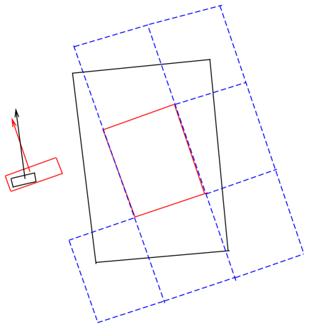
Figure 3. The boxes $\mathcal{C}^{*}_{\tau^{(\ell)}}$ and $K\mathcal{C}^{*}_{\tau^{(\ell-1)}}$.

Ir remains to show

$$\frac{1}{|\mathcal{C}^{*}_{\tau^{(k)}}|}\int_{\mathcal{C}^{*}_{\tau^{(k)}}}\psi^{4}_{:\tau^{(k)}:}(x)dx\lesssim R^{\varepsilon},\quad\text{for any }\varepsilon>0.$$

To prove this, we use the induction on $k$. We observe that the $L^{4}$ average of $\psi_{:\tau^{(1)}:}$ over $\mathcal{C}^{*}_{\tau^{(1)}}$ is bounded by $K^{4\alpha}_{1}$ in the first step. Assuming in the $(\ell-1)-$th stage, we already have

$$\Bigl{(}\frac{1}{|\mathcal{C}^{*}_{\tau^{(\ell-1)}}|}\int_{\mathcal{C}^{*}_{\tau^{(\ell-1)}}}\psi^{4}_{:\tau^{(\ell-1)}:}\Bigr{)}^{\frac{1}{4}}\lesssim K_{1}^{2\,\ell\,\alpha}.$$ (93)

Since $\psi_{:\tau^{(\ell)}:}=\psi_{:\tau^{(\ell-1)}:}\psi_{\tau^{(\ell)}}$, we need to evaluate

$$\frac{1}{|\mathcal{C}^{*}_{\tau^{(\ell)}}|}\int_{\mathcal{C}^{*}_{\tau^{(\ell)}}}\psi^{4}_{:\tau^{(\ell-1)}:}\psi^{4}_{\tau^{(\ell)}}(x)dx.$$ (94)

Because the angle between the two normal vectors of $\mathcal{C}_{\tau^{(\ell-1)}}$ at $\xi_{\tau^{(\ell-1)}}$ and $\mathcal{C}_{\tau^{(\ell)}}$ at $\xi_{\tau^{(\ell)}}$ is also controlled by $\frac{1}{K}$( see Figure 3), we may construct a cover of $\mathcal{C}^{*}_{\tau^{(\ell)}}$ by $K\mathcal{C}^{*}_{\tau^{(\ell-1)}}-$boxes as follows. Denote by $\{\mathcal{B}_{\rho}\}_{\rho}$ a collection of $\mathcal{C}^{*}_{\tau^{(\ell-1)}}-$boxes such that (see Figure 3)

$$\mathcal{C}^{*}_{\tau^{(\ell)}}\subset\bigcup_{\rho}K\mathcal{B}_{\rho}\subset 2\,\mathcal{C}^{*}_{\tau^{(\ell)}}.$$

On account of this, we can estimate

$$|\eqref{lth-target}|\lesssim\max_{\mathcal{B}_{\rho}}\frac{1}{|K\mathcal{B}_{\rho}|}\int_{K\mathcal{B}_{\rho}}\psi^{4}_{:\tau^{(\ell-1)}:}\psi^{4}_{\tau^{(\ell)}}(x)dx.$$

By the hypothesis of induction, we have

$$\int_{K\mathcal{B}_{\rho}}\psi^{4}_{:\tau^{(\ell-1)}:}\psi^{4}_{\tau^{(\ell)}}(x)dx \lesssim\sum_{\rho}(\psi_{\tau^{(\ell)}}|_{\mathcal{B}_{\rho}})^{4}\int_{\mathcal{B}_{\rho}}\psi^{4}_{:\tau^{(\ell-1)}:}(x)dx$$

$$\lesssim K_{1}^{8\alpha\ell}\sum_{\rho}(\psi_{\tau^{(\ell)}}|_{\mathcal{B}_{\rho}})^{4}|\mathcal{B}_{\rho}|$$

$$\lesssim K_{1}^{8\alpha\ell}\int_{K\mathcal{B}_{\rho}}\psi^{4}_{\tau^{(\ell)}}(x)dx$$

$$\lesssim K_{1}^{8\alpha(\ell+1)}|K\mathcal{B}_{\rho}|,$$

where in the last estimate, we used

$$\frac{1}{|K\mathcal{C}^{*}_{\tau^{(\ell-1)}}|}\int_{K\mathcal{C}^{*}_{\tau^{(\ell-1)}}}\psi^{4}_{\tau^{(\ell)}}(x)dx\lesssim K_{1}^{8\alpha}.$$

We denote

$$\delta=K^{-(\ell+1)},$$

and assume at the $\ell-$th stage

$$\frac{1}{\sqrt{R}}<\delta.$$

Noting that $K_{1}\ll K$ and

$$\ell+1=\log\frac{1}{\delta}/\log K,$$

we have

$$K_{1}^{8\alpha(\ell+1)}<R^{\frac{\log K^{4\alpha}_{1}}{\log K}}\ll R^{\varepsilon},\;\forall\;\varepsilon>0.$$

If $\delta$ ranges from all the dyadic numbers between $R^{-1/2}$ and $K^{-1}$, we see the contribution from all the type I terms is bounded by (3). The contributions from (85)(91) and (92) to (3) can be evaluated in a similar manner.

When the scale arrives at $\frac{1}{\sqrt{R}}$, the remainder term is bounded by (4). Finally, we lose an $R^{\varepsilon}-$factor by taking maximum in (3) and (4) with respect to dyadic $\delta\in(R^{-1/2},\,1/K)$. Thus, we complete the proof of Lemma 2.3.

Acknowledgements

We would like to appreciate Professor Sanghyuk Lee for indicating to us the recent work [CLV]. The authors were supported by the NSF of China under grant No.11231006 and 11371059.

References

- [1]
- [B1] J. Bourgain. A remark on Schrödinger operators, Isreal J. Math., 77(1992), 1–16.
- [B2] J. Bourgain, Some new estiamtes on osillatory integrals, Essays on Fourier Analysi in Honor of Elias M. Stein Princeton, NJ 1991. Princeton Math. Ser., Vol. 42, Princeton University Press, New Jersey, (1995), 83–112.
- [B3] J. Bourgain, On the Schrödinger maximal function in higher dimensions, Proceedings of the Steklov Institute of Mathematics, 280(2013), 46–60.
- [BG] J. Bourgain and L. Guth, Bounds on oscillatory integral operators based on multilinear estimates, Geom. Funct. Anal., 21(2011), 1239–1295.
- [BCT] J. Bennett, T. Carbery and T. Tao, On the multilinear restriction and Kakeya conjectures, Acta Math., 196(2006), 261–302.
- [Cr] L. Carleson, Some analystic problems related to statistical mechanics in Euclidean Harmonic Analysis, Lecture Notes in Math.,779, Springer Berlin(1979), 5–45.
- [CLV] C. Cho, S. Lee and A. Vargas, Problems on pointwise convergence of solutions to the Schrödinger equation, J. Fourier Anal. Appl. 18 (2012), no. 5, 972–994.
- [Co] A. Cordoba, Geometric Fourier analysis, Ann. Inst. Fourier , 32(1982), 215–226.
- [DK] B. Dahlberg and C.E. Kenig. A note on the almost everywhere behavior of solutions to the Schrödinger equations, Harmonic Analysis Lecture Notes in Math., 908, Springer, Berlin, (1982), 205–209.
- [H] L. Hörmander, Oscillatory integrals and multipliers on , Arkiv Math., 11(1973), 1–11.
- [KPV] C. E. Kenig, G. Ponce and L. Vega, Oscillatory integral and regularity of dispersive equations, Indiana University Math. Journal, 40(1991), 33–69.
- [L] S. Lee. On pointwise convergence of the solutions to Schrödinger equations in , Int. Math. Res. Not. (2006), 1–21.
- [LR] S. Lee and K. M. Rogers, The Schrödinger equation along curves and the quantum harmonic oscillator, Adv. Math. 229 (2012), no.3, 1359–1379.
- [M] A. Miyachi. On some singular Fourier multipliers, J. of the Faculty of Science. The Univ. of Tokyo. Sec. IA, 28(1981), 267–315
- [MVV] A. Moyua, A. Vargas and L. Vega. Schrödinger maximal function and restriction properties of the Fourer transform, IMRN , (1996), 793–815.
- [R] K. Rogers, A local smoothing estimate for the Schrödinger equation, Advances in Mathematics, 219(2008), 2105–2122.
- [S] P. Sjölin. Regularity of solutions to the Schrödinger equation, Duke Mathematical Journal, 55(1987), 699-715.
- [Sh] S. Shao. On Localization of the Schrödinger maximal operator, arXiv:1006.2787v1.
- [T1] T. Tao. Time-frequency harmonic analysis, http://www.math.ucla.edu/ tao/254a.1.01w/blurb.html
- [T2] T. Tao. A sharp bilinear restriction estiamte for parabloids, Geom. Funct. Anal., 13(2003), 1359–1384.
- [TV1] T. Tao and A. Vargas. A bilinear approach to cone multiplier.I.Restriction estiamtes. GAFA , 10(2000), 185–215.
- [TV2] T. Tao and A. Vargas. A bilinear approach to cone multiplier.II. Applications. GAFA , 10(2000), 216–258.
- [TVV] T. Tao, L. Vega and A. Vargas, A bilinear approach to the restriction and Kakeya conjectures J. Amer. Math. Soci. 11(1998), 967–1000.
- [V] L. Vega, Schrödinger equations: pointwise convergence to the initial data, Proceedings of the American Mathematical Society, 102(1988), 874–878.
- [W] T. Wolff, A sharp bilinear cone restriction estiamte, Ann. of Math., (2),153(3)(2001):661–698.