Spatiotemporal dynamics in 2D Kolmogorov flow over large domains

Abstract

Kolmogorov flow in two dimensions - the two-dimensional Navier-Stokes equations with a sinusoidal body force - is considered over extended periodic domains to reveal localised spatiotemporal complexity. The flow response mimicks the forcing at small forcing amplitudes but beyond a critical value develops a long wavelength instability. The ensuing state is described by a Cahn-Hilliard-type equation and as a result coarsening dynamics are observed for random initial data. After further bifurcations, this regime gives way to multiple attractors, some of which possess spatially-localised time dependence. Co-existence of such attractors in a large domain gives rise to interesting collisional dynamics which is captured by a system of 5 (1-space and 1-time) PDEs based on a long wavelength limit. The coarsening regime reinstates itself at yet higher forcing amplitudes in the sense that only longest-wavelength solutions remain attractors. Eventually, there is one global longest-wavelength attractor which possesses two localised chaotic regions - a kink and antikink - which connect two steady one-dimensional flow regions of essentially half the domain width each. The wealth of spatiotemporal complexity uncovered presents a bountiful arena in which to study the existence of simple invariant localised solutions which presumably underpin all of the observed behaviour.

1 Introduction

The problem of a 2-dimensional (2D) fluid on a torus $(x,y)\in[0,2\pi/\alpha]\times[0,2\pi]$ driven by monochromatic body forcing $\sin\,ny\,\hat{\mathbf{x}}$ with $n=1$ was first introduced by Kolmogorov in 1959 (Arnold & Meshalkin (1960); Arnol’d (1991)) as a mathematically and experimentally tractable flow situation in which to study instability and transition to turbulence. The linear instability of the steady, unidirectional base flow can be predicted analytically using continued fractions (Meshalkin & Sinai (1961)) and a remarkable global stability (or ‘anti-turbulence’) result is known for all forcing amplitudes when the forcing wavenumber, $n$, and box aspect ratio, $\alpha$, are both 1 (Marchioro (1986)). The flow can be realised in the laboratory either using electrolytic fluids (Bondarenko et al. (1979); Obukhov (1983); Sommeria (1986); Batchaev & Ponomarev (1989); Batchaev (2012); Suri et al. (2013)) or driven soap films (Burgess et al. (1999)). There are many possible variations of the problem: torus aspect ratio (e.g. Marchioro (1986); Okamoto & Shōji (1993); Sarris et al. (2007)), forcing wavelength ( e.g. She (1988); Platt et al. (1991); Armbruster et al. (1996)), forcing form (e.g. Gotoh & Yamada (1987); Kim & Okamoto (2003); Rollin et al. (2011); Gallet & Young (2013)), boundary conditions (Fukuta & Murakami (1998); Thess (1992); Gallet & Young (2013)), and 3-dimensionalisation (e.g. Borue & Orszag (2006); Shebalin & Woodruff (1997); Sarris et al. (2007); Musacchio & Boffetta (2014)). Further physics such as rotation, bottom friction and stratification (Lorenz (1972); Kazantsev (1998); Manfroi & Young (1999); Balmforth & Young (2002, 2005); Tsang & Young (2008, 2009)) can also be added to examine most commonly their effect on the inverse energy cascade in geophysical fluid dynamics. Recently compressible (Manela & Zhang (2012); Fortova (2013)), viscoelastic (Boffetta et al. (2005); Berti & Boffetta (2010)) and even granular (Roeller et al. (2009)) versions of Kolmogorov flow have been treated.

Mathematically, beyond the instability result of Meshalkin & Sinai (1961), past work has developed amplitude equations to study the dynamics near the bifurcation point (Nepomniashchii (1976); Sivashinsky (1985)) and used bifurcation analysis coupled with branch continuation techniques to uncover a variety of steady vortex states (Okamoto & Shōji (1993); Okamoto (1998); Kim & Okamoto (2003)). These solutions are qualitatively representative of the vortex arrays observed by numerous authors investigating transition to chaos in these types of flows (Obukhov (1983); Platt et al. (1991); Chen & Price (2004); Feudel & Seehafer (1995); Sarris et al. (2007)). However, with the exception of the bifurcation analysis of Okamoto (Okamoto & Shōji (1993); Okamoto (1996, 1998)), all of the work to date has avoided Marchioro’s 2D global stability result by considering a forcing wavenumber $n>1$ for $\alpha=1$, with $n=4$ being the most common choice (Platt et al. (1991); Chen & Price (2004); Chandler & Kerswell (2013)). The ensuing flow dynamics, at least at the low to intermediate forcing amplitudes studied, is then spatially global as the domain is square. The objective here is to extend these previous studies to spatially extended domains with $\alpha\leq\textstyle{1\over 4}$ in order to look for spatiotemporal behaviour.

The motivation for this study is the recent work by Chandler & Kerswell (2013) looking at 2D Kolmogorov flow over a small $[0,2\pi]^{2}$ domain. These authors attempt to make sense of the observed global chaos by extracting simple invariant sets or ‘recurrent flows’ (simple exact solutions of the Navier-Stokes equations) embedded in the chaos directly from their direct numerical simulations (DNS). The underlying idea is that the chaos as a whole can be viewed as one phase-space trajectory transiently visiting the neighbourhoods of simple invariants sets (equilibria, relative equilibria, periodic orbits and relative periodic orbits) which litter phase space. Assuming ergodicity, the properties of these simple invariant sets can then in principle be used, in some appropriately weighted fashion, to predict the statistical properties of the chaos. Due to the domain size used, Chandler & Kerswell (2013) naturally concentrated on extracting spatially-global recurrent flows from the (temporal) chaos. However the real challenge for practical applications is to consider larger domains where true spatiotemporal behaviour occurs in which the flow’s complexity can differ markedly in space at any given time. The hope in examining 2D Kolmogorov flow over an extended domain was that it would display spatially localised chaotic flows - i.e. something approaching 2D turbulence (spatial and temporal complexity) - and by implication possess spatially localised recurrent flows. This would then offer an ideal environment to develop further the recently-introduced techniques for extracting order and coherence from the apparent disorder of turbulence (Kawahara & Kida (2001); van Veen et al. (2006); Viswanath (2007, 2009); Cvitanović & Gibson (2010); Kreilos & Eckhardt (2012); Chandler & Kerswell (2013); Willis et al. (2013)).

The structure of the paper is as follows. A short formulation section sets the scene as considered previously in Chandler & Kerswell (2013) with the ‘geometry’ parameter $\alpha$ describing the aspect ratio of the computational domain now $\leq\textstyle{1\over 4}$. Section 3 describes the initial instability away from the steady, 1-dimensional (1D), unidirectional flow response realised at low forcing amplitudes. The new preferred steady flow state, which preserves the wavelength of the forcing but breaks its continuous translational symmetry, adopts the longest wavelength allowed. Beyond the initial bifurcation point, this state quickly develops into two 1D flow regions each over essentially half the domain joined together by a localised 2D transition regions (‘kinks’ and ‘antikinks’). A Cahn-Hilliard-like long-wavelength amplitude equation is discussed which explains this response and a more accurate 3-PDE long-wavelength system introduced. Further (primary) steady bifurcations off the basic state introduce initially-unstable states with more and more localised transition regions equally spaced across the domain. Section 4 details the existence of further steady and unsteady bifurcations and identifies the emergence of a global attractor at sufficiently high levels of forcing which displays localised chaos. Other disconnected states which arise in saddle node bifurcations are also found and the bifurcation structure of one is followed in detail from localised periodicity to chaotic attractor and then through a boundary crisis to a chaotic repellor where the chaos is then both spatially and temporally localised. Section 5 discusses the interesting behaviour observed when co-existing attractors interact in an even larger domain. A 5-PDE extension to the long-wavelength 3-PDE system, which adds the possibility of the kinks and antikinks developing structure, is successful in capturing the observed behaviour in the full system. In this 5-PDE system, the basic building blocks - families of travelling waves made up of various types of kink-antikink pairs with different separations and internal structures - are isolated. A final section 6 discusses the results and implications for further work.

2 Formulation

The incompressible Navier-Stokes equations with Kolmogorov forcing are given by

$$\frac{\partial\bm{u}^{*}}{\partial t^{*}}+\bm{u}^{*}\cdot\nabla^{*}\bm{u}^{*}+\frac{1}{\rho}\nabla^{*}p^{*} =\nu\Delta^{*}\bm{u}^{*}+\chi\sin(2\pi ny^{*}/L_{y})\bm{\hat{}}{\mathbf{x}},$$ (1)

$$\nabla^{*}\cdot\bm{u}^{*} =0$$ (2)

where $\bm{u}=u\hat{\mathbf{x}}+v\hat{\mathbf{y}}=(u,v)$ is the two-dimensional velocity field, $n$ is the forcing wavenumber, $\chi$ the forcing amplitude, $\nu$ kinematic viscosity, $p$ pressure and $\rho$ is the density of the fluid defined over the doubly periodic domain $(x,y)\in[0,L_{x}]\times[0,L_{y}]$. The system is then naturally non-dimensionalised with lengthscale $L_{y}/2\pi$ and timescale $\sqrt{L_{y}/2\pi\chi}$ to give

$$\frac{\partial\bm{u}}{\partial t}+\bm{u}\cdot\nabla\bm{u}+\nabla p =\frac{1}{Re}\Delta\bm{u}+\sin ny\,\bm{\hat{}}{x},$$ (3)

$$\nabla\cdot\bm{u} =0$$ (4)

where we define the Reynolds number

$$Re:=\frac{\sqrt{\chi}}{\nu}\left(\frac{L_{y}}{2\pi}\right)^{3/2}.$$ (5)

The equations are solved over $[0,2\pi/\alpha]\times[0,2\pi]$ where $\alpha=L_{y}/L_{x}$ defines the aspect ratio of the domain with always the choice $n=4$ here. For most of the runs presented here, $\alpha=\textstyle{1\over 4}$ but $\alpha=\textstyle{1\over 8}$ and exceptionally $\alpha=\textstyle{1\over 16}$ are considered too. For computational efficiency and accuracy we reformulate (3) so that vorticity $\omega:=\nabla\times\bm{u}$ is our prognostic variable and solve

$$\frac{\partial\omega}{\partial t}+\bm{u}\cdot\nabla\omega =\frac{1}{Re}\Delta\omega-n\cos ny.$$ (6)

The system has the symmetries

$$\mathcal{S}:[u,v](x,y) \rightarrow[-u,v]\left(-x,y+\frac{\pi}{n}\right),$$ (7)

$$\mathcal{R}:[u,v](x,y) \rightarrow[-u,-v]\left(-x,-y\right),$$ (8)

$$\mathcal{T}_{l}:[u,v](x,y) \rightarrow[u,v]\left(x+l,y\right)\qquad\textrm{for }0\leq l\leq\frac{2\pi}{\alpha},$$ (9)

where $\mathcal{S}$ represents the discrete shift-&-reflect symmetry, $\mathcal{R}$ rotation through $\pi$ and $\mathcal{T}_{l}$ is the continuous group of translations in $x$.

2.1 Flow measures

In order to discuss various features of the flows considered we define here some diagnostic quantities. Total energy, dissipation and energy input are defined in the standard way as

$$E(t):=\textstyle{1\over 2}\langle\bm{u}^{2}\rangle_{V},\qquad D(t):=\frac{1}{Re}\langle|\nabla\bm{u}|^{2}\rangle_{V},\qquad I(t):=\langle u\sin(ny)\rangle_{V}$$ (10)

where the volume average is defined as

$$\langle\quad\rangle_{V}:=\frac{\alpha}{4\pi}\int_{0}^{2\pi}\int_{0}^{2\pi/\alpha}{\rm d}x{\rm d}y.$$

The base state or laminar profile and its energy and dissipation are

$$\bm{u}_{lam}:=\frac{Re}{n^{2}}\sin ny\,\bm{\hat{x}},\qquad E_{lam}:=\frac{Re^{2}}{4n^{4}},\qquad D_{lam}:=\frac{Re}{2n^{2}}.$$ (11)

2.2 Numerical methods

The pseudospectral timestepping code presented in Chandler & Kerswell (2013) was ported into CUDA to allow accelerated calculations to be performed on GPUs. The algorithm itself remains identical, simply the implementation is altered to take advantage of the vast parallelism afforded by modern general purpose GPU cards (see the supplementary material for details). Vorticity is discretised via a Fourier-Fourier spectral expansion with resolution $N_{x}\times N_{y}$ and dealiased by the two-thirds rule such that

$$\omega(x,y,t)=\sum^{N_{x}/3-1}_{k_{x}=0}\sum^{N_{y}/3-1}_{k_{y}=-N_{y}/3}\Omega_{k_{x}k_{y}}(t)\mathrm{e}^{\mathrm{i}\left(\alpha k_{x}x+k_{y}y\right)}$$ (12)

together with reality condition $\Omega_{-k_{x}-k_{y}}=\Omega^{*}_{k_{x}k_{y}}$ (a mask is also used as outlined in section 3 of Chandler & Kerswell (2013)). Crank-Nicolson timestepping scheme is used for the viscous terms and Heun’s method for the nonlinear and forcing terms. As pointed out in Chandler & Kerswell (2013), this results in an algorithm that can be restarted from a single state vector which is very convenient for the various solution-finding algorithms employed here. Typical numerical resolutions used were 128 Fourier modes per $2\pi$ so $(N_{x},N_{y})=(512,128)$ for $\alpha=\textstyle{1\over 4}$ and $(1024,128)$ for $\alpha=\textstyle{1\over 8}$ (Chandler & Kerswell (2013) used 256 Fourier modes per $2\pi$ but tests showed they could easily have halved this as was done here). Typical time steps were $dt=0.05$ at $Re=20$ and $0.001$ at $Re=120$ with $2\times 10^{6}$ time steps ($dt=0.05$, $T=10^{5}$) of the $512\times 128$ grid for $\alpha=\textstyle{1\over 4}$ and $Re=20$ taking 63 minutes on a 512-core NVIDIA Tesla M2090 GPU.

In addition to the pseudospectral DNS (direct numerical simulation) code, we also made use of the Newton-GMRES-hookstep algorithm of Chandler & Kerswell (2013) in order to precisely converge any invariant states (steady states, travelling waves, periodic orbits and relative periodic orbits) that we came across. The only change from the code used in Chandler & Kerswell (2013) was the integration of the GPU accelerated timestepper. In contrast to Chandler & Kerswell (2013), the use of the technique in the current study was not to extract unstable solutions embedded in chaos, but simply to confirm simple attractors emerging from the simulations were actually exact solutions. We also employed their arc-length continuation algorithm to continue solution branches in $Re$.

Figure 1: DNS calculation from a randomised initial condition at $Re=10$ to show how the flow very slowly converges to the longest wavelength state. Shown on the left is the variation in $\omega$ in an $(x,t)$ plane for $y=21\pi/32$ and the right snapshots of $\omega(x,y)$ at $t=0,5\times 10^{3},10^{5}$ and $1.5\times 10^{5}$. Colour extrema are $\omega=-5$ black, $\omega=5$ white, and 5 evenly spaced contours in $-4\leq\omega\leq 4$ for $(x,y)$ plots and $-2\leq\omega\leq 2$ with 4 contours for $(x,t)$.

Figure 2: Profiles of vorticity at $y=\pi/8$ for $Re\gtrsim Re_{c}(\textstyle{1\over 4})=9.5416$ showing how the initial instability quickly generates a kink near $x=0$ and an antikink near $4\pi$.

3 Initial instability

The basic flow (11) is linearly unstable at a comparatively low $Re=Re_{c}$ with the exact value decreasing monotonically to a limiting value of $\sqrt[4]{2}n^{3/2}$ as the domain size $L$ becomes infinitely large. The asymptotic approximation (derived in the Appendix),

$$Re_{c}(\alpha)=\sqrt[4]{2}n^{3/2}\biggl{[}1+\frac{3\alpha^{2}}{4n^{2}}+O(\alpha^{4})\,\biggr{]},$$ (13)

illustrates this behaviour as $\alpha=2\pi/L\rightarrow 0$ (this formula is accurate to within $0.01\%$ at $\alpha=\textstyle{1\over 2}$).

For a given long domain $L$ and $Re$ in the interval $(\,Re_{c}(\alpha),Re_{c}(2\alpha)\,)$, the unique attractor is the steady solution branch which bifurcates supercritically at $Re_{c}(\alpha)$ and breaks the streamwise-independence of the basic state, i.e. the continuous symmetry $\mathcal{T}_{l}$, while preserving the discrete symmetries $\mathcal{S}$ and $\mathcal{R}$. Direct numerical simulations (DNS) for $\alpha=\textstyle{1\over 4}$ confirm this can stay a global attractor past $Re_{c}(2\alpha)=9.626$ up to 10.75. (Random initial data were used to initialise the DNS which means here that the code is started with uniform amplitudes but randomised phases for modes with $2.5<|k:=\sqrt{k_{x}^{2}+k_{y}^{2}}|<9.5$ - see (12) - normalised such that the total enstrophy is 1). A typical such run at $Re=10$ is shown in figure 1 where the system reaches the longest wavelength solution but only after a very long time. While the flow selects this longest overall wavelength, it also very quickly (as $Re$ increases) separates into 2D kink and antikink structures in the vorticity field (where length scales are $\partial_{x}=O(\partial_{y})$) which connect regions of essentially half the wavelength where the flow is 1D (independent of $x$). These 1D states take the form

$$\psi=\lambda x-\frac{Re}{n(Re^{2}\lambda^{2}+n^{2})}\cos ny+\frac{\lambda Re^{2}}{n^{2}(Re^{2}\lambda^{2}+n^{2})}\sin ny$$ (14)

where $\psi$ is the streamfunction ( $\bm{u}=(\psi_{y},-\psi_{x})$ ) and $\lambda$ is a parameter indicating the constant velocity in the $-\lambda\bm{\hat{y}}$ direction. We use the term ‘kink’ to refer to the 2D flow structure connecting a leftward (decreasing $x$) 1D state with a flow in the $-\bm{\hat{y}}$ direction to a rightward (increasing $x$) 1D state with flow in the $+\bm{\hat{y}}$ direction: the ‘antikink’ does the opposite. The localising 2D structure at the kink (antikink) then corresponds to coherent negative (positive) vorticity regions. Figures 2 and 3 both show an antikink in the centre of the flow domain and a kink at the end. Since the 1D solutions on either side of the kink and antikink have equal spatial extent, they must have equal in magnitude but oppositely signed $\lambda$ values to preserve the total linear momentum at zero in the $\bm{\hat{y}}$ direction. The kink and antikinks select the value for $\lambda$ as a function of $Re$ (or the domain size) with $\lambda$ increasing to the asymptotic value of $\lambda=\epsilon\sqrt{3\sqrt{2}/n}$ as the kinks and antikinks intensify: see the Appendix. Figure 3 shows the kink and antikink pair strengthening and localising although by $Re=25$ this flow structure is already no longer the global attractor.

Both the system’s preference for the longest wavelength instability and the generation of these kinks and antikinks can be captured in a long-wavelength approximation (Nepomniashchii, 1976; Sivashinsky, 1985) in which $\partial_{x}\ll\partial_{y}$ is assumed close to $Re=Re_{c}$. Briefly (see the Appendix for details), if

$$\frac{1}{Re}=(1-\epsilon^{2})\frac{1}{Re_{c}}$$ (15)

with $\epsilon\ll 1$ and the flow varies over the scale $X:=\epsilon x$, a streamfunction of the form

$$\psi = -\frac{Re_{c}(0)}{n^{3}}\cos ny+A^{0}(X,\epsilon^{4}t)+\epsilon\biggl{[}\frac{Re_{c}^{2}}{n^{4}}A_{X}^{0}\sin ny+A^{1}_{X}(X,\epsilon^{4}t)\biggr{]}$$ (16)

$$+\epsilon^{2}\frac{Re_{c}}{n}\biggl{[}-\frac{1}{n^{2}}\cos ny+(A^{0}_{X})^{2}\frac{Re_{c}^{2}}{n^{4}}\cos ny+\frac{Re_{c}}{n^{3}}A_{X}^{1}(X,\epsilon^{4}t)\sin ny\biggr{]}$$

$$+\epsilon^{3}\biggl{[}\biggl{(}\frac{3Re_{c}^{2}}{n^{6}}A_{XXX}^{0}+\frac{2Re_{c}^{2}}{n^{4}}A_{X}^{0}-\frac{Re_{c}^{4}}{n^{6}}(A_{X}^{0})^{3}+\frac{Re_{c}^{2}}{n^{4}}A_{X}^{2}(X,\epsilon^{4}t)\biggr{)}\biggr{.}\sin ny$$

$$\hskip 113.81102pt+\biggl{.}\frac{2Re_{c}^{3}}{n^{6}}A_{X}^{0}A_{X}^{1}\cos ny+A^{3}(X,\epsilon^{4}t)\biggr{]}+O(\epsilon^{4})$$

emerges with a solvability condition at $O(\epsilon^{3})$ giving the Cahn-Hilliard-type equation

$$A^{0}_{XXX}+\frac{4n^{2}}{3}A^{0}_{X}-\frac{2\sqrt{2}n^{3}}{9}(A_{X}^{0})^{3}=0$$ (17)

for the leading unknown amplitude function $A^{0}$. The appropriate solution of this is $A_{X}^{0}=\sigma$sn$(\beta X|k)$ where sn is the elliptic function and $\sigma,\beta$ and $k\in(0,1)$ are constants (see the Appendix for details). As $Re\rightarrow Re_{c}$, $k\rightarrow 0$ and $A_{X}^{0}$ tends to the expected $sine$ function whereas as $Re\rightarrow\infty$ ($k\rightarrow 1$) $A_{X}^{0}$ asymptotes to a $tanh$ function over each half wavelength mimicking the behaviour seen in figure 2. The preference for the longest wavelength of the system can be explained by the fact that all solutions to (17) are unstable to larger wavelengths disturbances (Nepomniashchii, 1976; Chapman & Proctor, 1980) so that only the solution already with the largest wavelength is stable.

Quantitative predictions for $v=-\psi_{x}$ are shown in figure 4 together with the actual DNS values at $\alpha=\textstyle{1\over 4}$ and $\alpha=\textstyle{1\over 16}$ near the bifurcation point. The $\alpha=\textstyle{1\over 16}$ DNS data is very close to the theory until $Re\approx 11$ whereas the $\alpha=\textstyle{1\over 4}$ DNS data differs near its bifurcation point but by $Re\approx 10$ is on top of the $\alpha=\textstyle{1\over 16}$ DNS data when the kinks have sufficiently localised. No prediction can be made for the vorticity without knowledge of $A^{1}(X,\epsilon^{4}t)$ which presumably is determined by the $O(\epsilon^{4})$ solvability condition. Rather than systematically deriving higher order amplitude equations in this way, we work with 3 (1-space and 1-time) coupled PDEs instead which automatically incorporate the first 4 amplitude functions and thereby give a much better long wavelength approximation.

Figure 3: Vorticity field $\omega$ (left) and streamfunction $\psi=-\nabla^{-1}\omega$ (right) for the $\mathcal{S}-$symmetric kink solutions at $Re=10,12,15,25$ in a domain $8\pi\times 2\pi$ to show how the kink and antikink intensify. Colour extrema for vorticity are $\omega=-5$ black, $\omega=5$ white, and 5 evenly spaced contours in $-4\leq\omega\leq 4$, while for streamfunction we use $\psi=-8$ black, $\psi=8$ white, and contours spaced by 0.5 in $-6\leq\psi\leq 6$.

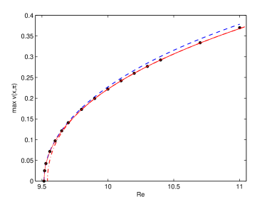
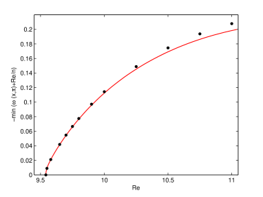
Figure 4: Left, a comparison of the theoretical prediction ($\alpha\rightarrow\infty$; blue-dashed line) and the DNS ($\alpha=\textstyle{1\over 16}$; red solid line) for $\max_{x}\,v(x,\pi)$. The black dots are the results from the 3-PDE system. Numerical data for $\alpha=\textstyle{1\over 4}$ is also shown as a red dash-dot line which only differs from the $\alpha=\textstyle{1\over 16}$ line near their (different) bifurcation points. Right, the predictions of the 3-PDE systems (black dots) and the DNS data (red solid line) for $\min_{x}(\omega(x,\pi)+Re/n)$ in a domain $8\pi\times 2\pi$.

3.1 3-PDE long-wavelength system

The streamfunction (16) which emerges out of the long wavelength approximation involves just zero or first harmonics of the forcing’s periodicity in $y$ up to and including $O(\epsilon^{3})$ (higher harmonics $\sin 2ny$ and $\cos 2ny$ start to appear at $O(\epsilon^{4})$). Hence, rather than working with a sequence of amplitude equations for $A^{0}$, $A^{1}$, $A^{2}$ and $A^{3}$, it is simpler to assume the streamfunction takes the form

$$\psi(x,y,t)=\biggl{(}-\frac{Re}{n^{3}}+g(x,t)\biggr{)}\cos ny+h(x,t)\sin ny+\int^{x}F(\xi,t)d\xi$$ (18)

and work directly with the functions $g$, $h$ and $F$. Defining the associated vorticities as $\omega_{F}:=-F^{{}^{\prime}}$, $\omega_{g}:=-(g^{{}^{\prime\prime}}-n^{2}g)$ and $\omega_{h}:=-(h^{{}^{\prime\prime}}-n^{2}h)$ where $(\quad)^{{}^{\prime}}$ indicates a derivative with respect to $x$, the higher order long wavelength system is then simply the 3 (1-space and 1-time) PDEs

$$\frac{\partial\omega_{F}}{\partial t} = \frac{1}{Re}\omega_{F}^{{}^{\prime\prime}}+\frac{Re}{2n^{2}}(n^{2}h-\omega_{h})^{{}^{\prime}}+\textstyle{1\over 2}n(g\omega_{h}-h\omega_{g})^{{}^{\prime}},$$

$$\frac{\partial\omega_{g}}{\partial t} = \frac{1}{Re}(\omega_{g}^{{}^{\prime\prime}}-n^{2}\omega_{g})+nF\omega_{h}-nh\omega_{F}^{{}^{\prime}},$$

$$\frac{\partial\omega_{h}}{\partial t} = \frac{1}{Re}(\omega_{h}^{{}^{\prime\prime}}-n^{2}\omega_{h})+\frac{Re}{n^{2}}(n^{2}F-\omega_{F}^{{}^{\prime}})+n(g\omega_{F}^{{}^{\prime}}-F\omega_{g}).$$ (19)

as opposed to the original 2 (2-space and 1-time) Navier-Stokes PDEs. As expected, this system produces a better long wavelength prediction for $v$ than that available from (17) and can yield a prediction for the vorticity too (see figure 4). Its real use here, however, (although see section 5 later) is in studying the initial bifurcation of the flow without the constraining influence of periodic boundary conditions (coding up the 3 time-dependent PDEs is straightforward using second-order finite differences - Crank-Nicolson for the diffusive terms and Adams-Bashforth for the advective terms - and typically 250-500 grid points per $2\pi$ length). The non-periodic boundary conditions which do not allow energy to enter or leave the domain are

$$g^{{}^{\prime}}=h^{{}^{\prime}}=\omega_{g}^{{}^{\prime}}=\omega_{h}^{{}^{\prime}}=\omega_{F}=\omega_{g}^{{}^{\prime}}=\omega_{h}^{{}^{\prime}}\biggl{|}_{x=0,L}\biggr{.}=0\quad{\rm\&}\quad\overline{F}:=\int^{L}_{0}F\,dx={\rm const}$$ (20)

which represents conservation of momentum perpendicular to the forcing direction (in the DNS code $\overline{F}=0$ by construction). As way of confirmation, a linear stability analysis of the system (19) & (20) around $(F,g,h,\omega_{F},\omega_{g},\omega_{h})=0$ gives the same value of $Re_{c}$ as the periodic domain of twice the length (half of the wavelength of the periodic instability fits into the non-periodic domain). In this system, it is possible to confirm the localised nature of the vorticity kinks and antikinks although direct time stepping to these attractors is very inefficient due to the metastability of intermediate states (as indicated in figure 1). However, a Newton-Raphson solver converges easily given a reasonable starting guess from time stepping: see figure 5.

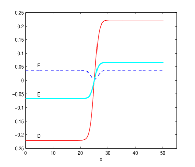
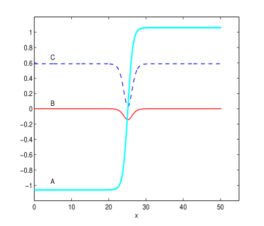
Figure 5: The antikink solution at $Re=10$ in a domain $16\pi\times 2\pi$ ($\alpha=\textstyle{1\over 8}$) as calculated in the 3-PDE system with non-periodic boundary conditions and 4000 grid points confirming localisation. The left plot shows $F$ (red), $g$ (blue dashed) and $h$ (thick cyan), and the right plot shows $\omega_{F}$ (red), $\omega_{g}$ (blue dashed) and $\omega_{h}$ (thick cyan).

Figure 6: Dissipation against Reynolds number for $\alpha=\textstyle{1\over 4}$, $n=4$ Kolmogorov flow. Curves indicate different $\kappa=m\alpha$ solutions together with P1 and P2 solution branches. Thick solid lines represent stable solutions, dashed are unstable. Point (a) indicates the first solution, $k=2\alpha$, becomes stable at $Re=10.75$ after bifurcating supercritically from the laminar flow. For the $\kappa=\alpha$ solution, the black curve represents the stable main secondary branch bifurcating at (b) $Re=15$.

Figure 7: Vorticity fields for the ‘uneven’ $\mathcal{R}$-asymmetric, $\mathcal{S}$-symmetric kink solutions ( which bifurcate off the primary $\kappa=2\alpha$ branch) at $Re=12$ (left) and 25 (right). Colour extrema are $\omega=-5$ black, $\omega=5$ white, and 5 evenly spaced contours in $-4\leq\omega\leq 4$.

Figure 8: Vorticity fields for the primary solutions $\kappa=2\alpha,4\alpha,6\alpha,8\alpha$ at $Re=25$ in the $8\pi\times 2\pi$ ($\alpha=\textstyle{1\over 4}$) domain. Colour extrema are $\omega=-5$ black, $\omega=5$ white, and 5 evenly spaced contours in $-4\leq\omega\leq 4$.

4 Bifurcations in the $8\pi\times 2\pi$ ($\alpha=\textstyle{1\over 4}$) domain

We now consider bifurcations in a $8\pi\times 2\pi$ ($\alpha=\textstyle{1\over 4}$) domain. Bifurcated solutions off the basic state (11) are referred to as primary solution branches, bifurcations off these primary branches are termed secondary solution branches and so on for tertiary solutions. Solutions can either have the wavelength of the domain or have multiple wavelengths within the domain. To indicate this, the smallest (base) wavenumber of the solution, $\kappa$, is expressed as a multiple of $\alpha$: a $\kappa=m\alpha$ solution has $m$ wavelengths across the domain so that in the representation (12) $k_{x}=0,\pm m,\pm 2m,\ldots$. Stability results are computed via Arnoldi iteration (using ARPACK) of the Jacobian matrix constructed during the Newton-GMRES-hookstep continuation.

4.1 Steady bifurcations

As stated above, the $\kappa=\alpha$ primary solution branch, which bifurcates supercritically off the base flow (11) at $Re_{c}(\alpha)=9.542$, is steady and found to be the unique attractor up to $Re=10.75$. At this point (point (a) in figure 6), the $\kappa=2\alpha$ primary solution branch, which bifurcates off the base flow at $Re(2\alpha)=9.626$, gains stability through a $\mathcal{R}-$breaking bifurcation. The new unstable secondary branch - hereafter christened the ‘uneven’ branch - is characterised by the uneven distribution in $x$ of the two kink-antikink pairs across the domain. The two antikinks and one kink quickly aggregate to form one composite antikink with much more structure than the remaining kink: see figure 7. This bifurcation is significant in that it results in coexisting, locally attracting states for the first time and thereby provides an upper limit on where the long-wavelength approximation - or ‘coarsening regime’ in Cahn-Hilliard language - is useful. The vorticity of the $\kappa=2\alpha$ primary solution and other primary solutions with $\kappa=4\alpha$, $\kappa=6\alpha$ and $\kappa=8\alpha$ are shown in figure 8.

Figure 9: Rescaled dissipation $Re^{2}D/D_{lam}\propto\langle|\nabla\bm{u}|^{2}\rangle_{V}$ against $Re$ for steady primary and secondary solutions branches. Black dots correspond to vorticity fields in figure 10.

Figure 10: Vorticity fields for steady $\kappa=\alpha$ solutions at $Re=24$, left, and $Re=45$, right. Ordered from bottom to top in ascending dissipation ($D$) corresponding to black dots in figure 9. Colour extrema for vorticity are $\omega=-5$ black, $\omega=5$ white, and 5 evenly spaced contours in $-4\leq\omega\leq 4$. The states shown on the right have been chosen to illustrate (from top down to the bottom) both kink and antikink trying to localise, 2 localisation events in antikink, little localisation, only localisation in the kink and kink more localised than the antikink.

Figure 11: Vorticity fields for the primary $\kappa=\alpha$ branch (left) and the main secondary branch (right) at $Re=141$. Colour extrema are $\omega=-15$ black, $\omega=15$ white, and 5 evenly spaced contours in $-10\leq\omega\leq 10$.

Figure 12: Left plot shows rescaled dissipation $Re^{2}D/D_{lam}$ against $Re$ for the solutions shown in figure 9 but now for $Re>60$ (red $\mathcal{S}$-symmetric primary branch and black main secondary $\mathcal{S}$-asymmetric branch, all line colours correspond to those in figure 9 ) and time dependence displayed as local minima in DNS time series (orange points). Right shows a typical segment from the time series at $Re=72$ (black solid line) and $Re=90$ (blue dashed line) with circles indicating minima as shown in the left hand plot. At $Re=120$, (a) indicates the the primary $\kappa=\alpha$ branch, the middle grey line, labelled (c), corresponds to the second state up on the right state in figure 10, and the upper black line, labelled (b) is the $\kappa=\alpha$ secondary branch drawn as the top black line in 9 into which the main $\kappa=\alpha$ secondary branch terminates at $Re\approx 80$. Note the other solution branches either terminate at other branches or can’t be continued due to lack of numerical convergence.

Figure 13: DNS calculation at $Re=120$ which shows the chaotic oscillation of the kinks. Shown on the left is the variation in $\omega$ in an $(x,t)$ plane for $y=21\pi/32$ and the right corresponding snapshots of $\omega(x,y)$ at $t=50$ (bottom), $t=250$ (middle) and $t=350$ (top). Colour extrema are $\omega=-8$ black, $\omega=8$ white, and 5 evenly spaced contours in $-8\leq\omega\leq 8$ for $(x,y)$ plots.

Figure 14: Variation in $\omega$ in an $(x,t)$ plane for $y=21\pi/32$. Top shows chaotic attractors for $\alpha=1.1$ (left) and $\alpha=1$ (right), bottom left shows the translating and oscillating kinks for $\alpha=0.9$ and right the steady translating kinks for $\alpha=0.75$. All four are at $Re=40$ and are over a temporal window of $T=10^{3}$ following a longer run of $10^{4}$ time units to eliminate transients. Colours are $-3\leq\omega\leq 3$ black to white.

The primary $\kappa=\alpha$ solution becomes unstable at $Re\approx 15$ through two very close but separate $\mathcal{S}-$symmetry breaking (modulational) bifurcations at $Re\approx 14.944$ and $Re\approx 14.946$ each giving rise to two new distinct secondary solution branches (point (b) in figure 6). Figure 9 shows all four new secondary branches and (a subset of the) subsequent tertiary bifurcations over $15\leq Re\leq 55$ produced via arc-length continuation (a rescaled dissipation is plotted to draw out the variation in the solution curves which are compressed in a $D$ vs $Re$ plot: see figure 6). The primary $\kappa=\alpha$ solution is the lowest (red) branch over $15\lesssim Re\lesssim 30$ in figure 9 and the middle thick (black) line indicates one of the new secondary $\mathcal{S}-$asymmetric branches - hereafter the ‘main secondary branch’ - which is found to be attracting from its birth near $Re=15$ up to $Re=32$ with only a small window of instability $24.97<Re<25.23$ (stable solutions are shown using solid lines and unstable solutions using dashed lines in Figure 9). Plots of the vorticity fields associated with the secondary branches (figure 10) indicate how the solutions vary subtly in their kink and antikink structures. The fact that kinks and antikinks of different ‘internal’ ($y$) structure can be paired together will be discussed again in section 5. A selection of tertiary solutions at $Re=45$ are also shown in the same figure to illustrate the variety of states which arise. The trend is for the vorticity to accumulate in the largest $y$-scale with the states varying in how effectively this has occurred and whether it is happening equally in both kink and antikink or just one. The primary $\kappa=\alpha$ branch and its secondary solutions can be continued to much higher $Re$ (where they are unstable) and then the contrast in their vorticity structure becomes dramatic: see figure 11.

The stability of the multiple wavelength primary solutions is summarised in figure 6. After gaining stability at $Re=10.75$, the $\kappa=2\alpha$ primary branch becomes unstable again at $Re=14.9$ through a modulational instability. The new solution branches were not studied in detail and so only one secondary branch (the ‘uneven’ solution) is shown in figure 6. The $\kappa=4\alpha$ primary solution has a window of stability of $11.2<Re<14.0$, the $\kappa=6\alpha$ primary solution is stable over $11.9<Re<13.1$ and the $\kappa=8\alpha$ primary solution is stable over $13.3<Re<13.78$.

4.2 Unsteady bifurcations

Along the main $\kappa=\alpha$ secondary solution (thick black line in figure 9), a Hopf bifurcation occurs at $Re\approx 32$. A sweep of DNS is then performed from this bifurcation point, moving in increments of $Re=0.5$ where the previous endstate (after a total time of $T=5\times 10^{4}$) is used to initiate the next run. Periodic orbits are observed in the range $32\leq Re\leq 50$ after which the main $\kappa=\alpha$ secondary solution becomes stable again over the interval $50\leq Re\leq 64$ (verified via Arnoldi). For $64<Re<69$, we observe a return to periodic behaviour based around the main secondary branch until there is a window of chaos for $69\leq Re<77$: see figure 12 (and supplementary video 1). Periodicity reappears for $77\leq Re<102$, a narrow window of quasiperiodicity follows before sustained ‘kink-antikink’ chaos sets in for $Re>103$. Figure 13 shows a space-time plot of this chaos which is localised and some snapshots of the flow illustrating this at $Re=120$. This state appears to be the global attractor for $Re>120$; five different randomised initial conditions were simulated at $Re=200$ for $10^{4}$ time units and all settle upon the same $\kappa=\alpha$ kink-antikink chaotic attractor. We suspect that the transition to sustained kink-antikink chaos at $Re=103$ also indicates the threshold of this uniqueness.

4.3 Kinks & antikinks in smaller domains

The ubiquity of these kink and antikink structures in sufficiently large domains (where they can be easily recognised) poses the question whether they are also relevant to the dynamics in smaller domains and therefore previous work. The chaos previously studied in 2D Kolmogorov flows has taken the form of spatially global states (Platt et al. (1991), Chen & Price (2004), Chandler & Kerswell (2013)) in a small $2\pi\times 2\pi$ domain. However, it is possible to pick out the presence of kink-antikink pairs even here. Figure 7 from Chandler & Kerswell (2013) shows some steady and travelling wave states at $Re=40$ which are strikingly similar to the $\mathcal{S}$-asymmetric branches shown in figure 9. In addition (their) figures 10 and 12 show unstable periodic orbits which seem to consist of a coherent kink-antikink pair closely interacting (see also figure 24(b) in Balmforth & Young (2002)). Decreasing $\alpha$ from slightly above $1$ to below 1 has the dramatic effect of letting the kink and antikink separate: see Figure 14 which shows $\omega(x,21\pi/32,t)$ in the $(x,t)$ plane for $Re=40$ and $\alpha=1.1$, $1$, $0.9$ and $0.75$. For $\alpha=1.1$, the flow is organised into alternate signed strips of vorticity (kinks and antikinks) which chaotically oscillate and meander but are never able to spatially separate. This dynamics is repeated at $\alpha=1$ but is noticeably less intense. Intermittently the kink and antikink undergo a more violent interaction which is discussed in Chandler & Kerswell (2013) as high dissipation excursions or ‘bursts’. When $\alpha$ is reduced to $0.9$, the character of the flow changes considerably as the kink-antikink separation increases and a coherent structure forms, oscillating and translating in a regular fashion. A further expansion of the domain ($\alpha=0.75$), produces an even simpler attractor where the kink-antikink pair, now quite separated, just translates to the left with constant speed.

Figure 15: DNS calculation from a randomised initial condition at $Re=20$ which shows kink-antikink annihilation events. Shown on the left is the variation in $\omega$ in an $(x,t)$ plane for $y=21\pi/32$ and the right snapshots of $\omega(x,y)$ at (from bottom to top) $t=1.25\times 10^{4},5\times 10^{4},7.5\times 10^{4},8.5\times 10^{4}$ and $10^{5}$. Colour extrema are $\omega=-5$ black, $\omega=5$ white, and 5 evenly spaced contours in $-4\leq\omega\leq 4$ for $(x,y)$ plots and $-3\leq\omega\leq 3$ for $(x,t)$.

Figure 16: Vorticity fields for the $Re=20$ P1 orbit (period $T=20.61$) at $t=0,3.5,7,10.5,14,17.5$, colour extrema are $\omega=-5$ black, $\omega=5$ white, and 5 evenly spaced contours in $-4\leq\omega\leq 4$ in a $8\pi\times 2\pi$ domain. The bordering kink/antikink look steady whereas the central snake oscillates periodically.

Figure 17: Dissipation minima for DNS of the P1 solution branch taken from $T=10^{5}$ time series shown in black. Light green curve shows $\kappa=2\alpha$ primary steady state. At $Re\approx 21.15$ we observe a torus bifurcation and quasi-periodic behaviour thereafter with occasional returns to periodic orbits, and full chaos at $Re=24$. For $T=10^{5}$, $Re=24.15$ is the first transient DNS along this sweep, however we find longer runs at $Re=24.1$ are also transient indicating that the boundary crisis occurs between $24.05$ and $24.1$. Note we only plot 1% of minima points to clearly indicate the structure of the various attractors. The post crisis transient DNS is shown in light blue (rightmost line of data) and periodic orbits are shown in magenta (light grey in b/w).

4.4 P1: a disconnected solution

Randomly-seeded DNS runs at $Re=20$ uncovered a new stable time-periodic solution - hereafter labelled P1 - coexisting with a steady kink-antikink solution at $Re=20$. Figure 15 documents one such run showing the familiar kink-antikink annihilation or coarsening events but, rather than reaching the steady main $\kappa=\alpha$ secondary branch, the final attractor is the new P1 state (note it took $O(10^{5})$ time units to settle). This solution appears to consist of a direction-reversing travelling wave (Landsberg & Knobloch (1991)) flanked by a steady kink and antikink: see figure 16 and video 2. Landsberg & Knobloch (1991) describe how a Hopf bifurcation from a circle of steady states due to $O(2)$ symmetry gives rise to an oscillatory drift along the group orbit of these steady states (e.g. Alonso et al. (2000)). There is certainly $O(2)$ symmetry present - $\mathcal{R}\times\mathcal{T}_{l}$ - but the flanking kink and antikink do not appear to move: see figure 16. This suggests that P1 has arisen through a Hopf bifurcation off a steady localised state with $O(2)$ symmetry contained between the kink and antikink rather than the whole global state. However this could not be confirmed because in this domain P1 does not bifurcate off a steady state but instead is born in a saddle node bifurcation (see below).

To confirm P1 was an exact solution and not a long-lived transient, the Newton-GMRES-hookstep method described in Chandler & Kerswell (2013) was used successfully to converge it as a ‘relative’ periodic solution of the Navier-Stokes equations. A ‘relative’ periodic orbit is a flow which repeats after a period $T$ and a drift in any homogeneous direction of the system (see Chandler & Kerswell (2013) for more discussion). At $Re=20$, the $L^{2}$ norm of the difference between the velocity fields separated by a period $T=20.61$ and a shift in $x$ of $-0.0002$ normalised by the $L^{2}$ norm of the starting field was reduced to zero to machine accuracy. Once converged, P1 could be traced using arc-length continuation over the range $15.03\leq Re\leq 26.68$ (at either end the Newton-GMRES-hookstep algorithm fails to converge).

Near $15.03$, the solution branch becomes close to the primary $\kappa=2\alpha$ solution (which has 2 kink-antikink pairs in a $8\pi\times 2\pi$ domain) as is perhaps to be expected since the oscillatory centre of the P1 looks to be made up of a kink-antikink pair. However, no connection was found and instead a partner branch of periodic solutions is found consistent with a saddle node bifurcation. To explore the stability of P1 and what happens to it beyond $Re=26.68$, a sweep of DNS was undertaken starting from the $Re\approx 17$ stable snake and incrementing $Re$ in $0.05$ steps. Initial conditions were taken to be the end state of the previous $Re$ run and each run was integrated for $T=10^{5}$. The nature of the solutions found is illustrated by plotting local minima of dissipation $D_{min}$ from the time series against $Re$ in figure 17. The first bifurcation experienced by P1 is period-doubling which occurs at $Re=17.8$. After a number of further period doublings, there is a torus bifurcation at $Re\approx 21.15$ indicated by the start of line filling in figure 17 when the dissipation minima are plotted. The difference in the power spectra before (at $Re=20$ with one fundamental frequency of $0.30$) and after (at $Re=22.1$ where there are two fundamental frequencies $0.438$ and $0.064$ given dominant peaks in the spectrum at $0.438$ and $0.502$) this bifurcation is clear from figure 18 as well as from the Poincaré sections in figure 19. Thereafter trajectories appear to be embedded in such tori with sporadic returns to periodic behaviour with the most notable being the interval $23.25\leq Re\leq 23.5$ (see figure 17). For $Re>23.5$, the quasiperiodicity returns followed by a chaotic regime at $Re=24$ (see figures 18 and 19), a periodic orbit at $Re=24.05$ and then an apparent boundary crisis at $Re=24.1$ whereupon the state becomes transient.

Figure 18: Power spectra for the time dependent signals of $D/D_{lam}$ taken from the final $10^{4}$ time units of the P1 DNS sweep illustrated in figure 17. $Re=20$, $22.1$, $24.1$, $23.5$ moving clockwise from top left.

Figure 19: Poincare sections for trajectories from the P1 DNS sweep illustrated in figure 17. The intersecting plane is taken to be cutting $D-I=0$ from below and we plot the variation in the $k_{y}=1,2,$ $k_{x}=0$ components (chosen to negate the effect of $x$-translation). The final 1000 time units are taken and we show $Re=20$, $22.1$, $24$, $23.5$ moving clockwise from top left. These sections nicely highlight the periodicity, quasi-periodicity and chaos of the attractors at these Reynolds numbers.

4.5 Boundary crisis for P1

Given the recent interest in transient turbulence in wall-bounded shear flows (e.g. Avila et al. (2011) and references therein) and the fact that for $Re\approx 24.1$ P1 appears to offer a simpler 2D spatially-localised version, this transient state was examined further. The growing range of the dissipation minima shown in figure 17 as $Re$ approaches the chaotic attractor-repellor transition points towards a boundary crisis in which the chaotic dynamics have grown with $Re$ to collide with its basin boundary. To corroborate this hypothesis, lifetimes of trajectories initiated in the former attractor were computed. A 1-D cross-section of initial conditions across the former attractor was generated by taking the periodic orbit converged at $Re=23.5$, $\omega_{1}(\bm{x},t)$, and systematically rescaling it as follows

$$\omega_{\lambda}(\bm{x},t=0)=\lambda\omega_{1}(\bm{x},t=0)$$

where $\lambda$ is some real number such that $\lambda=1$ should be in the attractor pre-crisis and for sufficiently larger and smaller values, trajectories of $\omega_{\lambda}$ will exit (leading to quick convergence to the kink attractor). The lifetime within the attractor, $\tau$, is defined as the time until the normalised dissipation $D(t)/D_{lam}$ falls below some threshold deemed to be outside the basin of attraction. Given at $Re\geq 24.1$ we observe trajectories attracted to the main $\kappa=\alpha$ secondary solution, which has significantly lower dissipation, the lifetime threshold is set to be $D_{tresh}=0.07$ (see figure 17). The total time integration is capped at $T=10^{5}$ and 100 steps are taken in $\lambda$ across the interval $[0.76,1.16]$. Pre-crisis at $Re=24$, all initial conditions $0.8\lesssim\lambda\lesssim 1.15$ stay in the attractor (over the $10^{5}$ time interval) whereas post-crisis at $Re=24.2$, the lifetimes vary enormously across the small steps taken in $\lambda$ consistent with a chaotic saddle: see figure 20. As a further check, a chaotic saddle should exhibit lifetimes which are exponentially distributed indicating that the probability of leaving the saddle in a given time period depends only on the length of the period. Checking this property, however, requires extensive DNS to build up enough data and as a result was not pursued further. In figures 21 (see video 3) and 22 (left), we show a typical ending for the chaotic saddle at $Re=24.1$. Efforts to analyse this chaotic saddle and attractor using the recurrent-flow analysis performed in Chandler & Kerswell (2013) will be reported elsewhere.

Figure 20: Lifetimes for the P1 chaotic attractor at $Re=24$ (blue circles) and chaotic transient at $Re=24.2$ (black $+$) against $\lambda$, the initial condition scaling. Also plotted as a dashed red line is the mean lifetime $\bar{\tau}=35,488.7$ for transient trajectories at $Re=24.2$.

Figure 21: Variation in $\omega$ in an $(x,t)$ plane for $y=21\pi/32$. Left shows the P1 chaotic attractor at $Re=24$ to $T=10^{5}$ and right shows a shorter time integration ($T=2\times 10^{4}$) for the chaotic saddle at $Re=24.1$. Colours are $-2\leq\omega\leq 2$ black to white.

Figure 22: Left shows vorticity fields for the $Re=24.1$ P1 chaotic transient at $t=12000,14000,14500,15000$ (bottom to top), showing the departure from the chaotic saddle by $t=15000$. Right shows vorticity fields for the $Re=20$ P2 periodic orbit (period $T=21.42$) at $t=0,5,10,15$ (bottom to top). Colour extrema are $\omega=-5$ black, $\omega=5$ white, and 5 evenly spaced contours in $-4\leq\omega\leq 4$.

4.6 P2: another disconnected solution

In addition to the P1 solution discovered as an attractor at $Re=20$, further DNS runs lead to another related solution stable for $Re\lesssim 21$. This orbit - labelled P2 - has period $T=21.42$ and $x$-shift $s=-0.0015$ at $Re=20$ and has two regions of spatially-localised oscillations: see figure 22 (right) and video 4. It is distinct from P1 which only has its oscillatory part in the region where the fluid is moving in the $-\bm{\hat{y}}$ direction. P2 has an oscillatory region in both the $-\bm{\hat{y}}$ and $+\bm{\hat{y}}$ moving regions (see also figure 6). Exploratory computations indicate that P2 undergoes a similar bifurcation sequence to (attractive) chaos before becoming a chaotic repeller. For $25\lesssim Re$, the only attractors found were longest-wavelength solutions in which a single kink-antikink pair exist and have a variety of time-dependent behaviours but with no mean motion.

Another long-lived but ultimately transient state was also found at $Re=20.75$ and is shown in figure 23 for $t<7.5\times 10^{4}$ (see video 5). This state has two spatially localised time-dependent patches within the same flanking kink-antikink pair and appears chaotic before ultimately settling down to P1 (no attempt was made to identify a stable version of this state by reducing $Re$). The evolution shown in figure 23 (left) highlights the differing translational speeds of this chaotic transient and P1. The co-existence of apparently-localised flow structures with different translational speeds begs the question: in a large domain where they can coexist spatially, what will happen when they collide?

Figure 23: DNS calculation at $Re=20.75$ showing a double oscillation long-lived transient. Shown on the left is the variation in $\omega$ in an $(x,t)$ plane for $y=21\pi/32$ and the right snapshots of $\omega(x,y)$ at (from bottom to top) $t=2.5\times 10^{4},5\times 10^{4},7.5\times 10^{4}$ and $10^{5}$. Colour extrema are $\omega=-5$ black, $\omega=5$ white, and 5 evenly spaced contours in $-4\leq\omega\leq 4$ for $(x,y)$ plots and $-2\leq\omega\leq 2$ for colours in $(x,t)$.

5 Behaviour in a $16\pi\times 2\pi$ ($\alpha=\textstyle{1\over 8}$) domain

To investigate the possibility of different flow structures interacting, some exploratory DNS calculations were performed with randomised initial data in an extended $16\pi\times 2\pi$ domain ($\alpha=\textstyle{1\over 8}$). At $Re=20$ and $25$, the initial data gradually evolved into the familiar secondary $\kappa=\alpha$ solution but at $Re=22$, differentially-propagating localised states quickly emerged out of the initial data. These interacted and ultimately formed a periodic state in which kinks and antikinks repeatedly collide. Figure 24 shows the total time history on the left and some selected snapshots of the vorticity field on the right (see video 6). At $t=3.4\times 10^{4}$, there is a state resembling a compressed version of P1 propagating slowly in the positive $x$-direction and a kink and antikink some distance apart to the right of it. At $4.85\times 10^{4}$, the P1-like state has broken down into a kink-antikink pair making a total of two pairs in the domain. One pair has become close and propagates as a coherent unit with constant speed. When this antikink-kink pair collides with the stationary antikink (e.g. $t=4.95\times 10^{4}$) from the left, the leftmost antikink becomes stationary and a new kink-antikink pairing is created which then moves off at the same speed after the ‘collision’ (e.g. $t=5.05\times 10^{4}$). This swapping phenomenon repeats periodically in time, due to the periodic boundary conditions. The period was too large to converge using the Newton-GMRES-hookstep method.

The interaction of these kinks and antikinks can be more complicated. Using the final state calculated at $Re=22$ as an initial condition for a DNS at $Re=18$, we find that the kinks and antikinks can rebound rather than colliding: see figure 25. Interestingly, there is some adjustment in the internal structure of the kink-antikink pair after this episode presumably to produce the reversal in propagation speed. There is also more separation between the kink and antikink in this pairing compared to that found at $Re=22$ and the propagation speed is correspondingly smaller.

Repeating the exercise at $Re=19$, figure 26 (see also video 7) shows three different types of behaviour in one run. The first is a kink-antikink partner swap at $t\approx 7\times 10^{3}$ (as per figure 24), then two rebounds at $2.2\times 10^{4}$ and $3.95\times 10^{4}$ (as per figure 25) and then finally, a fusion of a kink-antikink pair with a stationary kink which leads to a complicated oscillating structure reminiscent of the central part of P1. The endstate is then a stationary antikink separated from a non-propagating kink-antikink-kink chaotic structure.

For $25\lesssim Re$, DNS initiated with random initial conditions were found to invariably settle to a longest-wavelength ($\kappa=\alpha$) kink-antikink solution. Therefore, as in the $8\pi\times 2\pi$ domain, the coarsening regime re-establishes itself albeit now with a variety of local longest-wavelength attractors.

Figure 24: DNS calculation for randomised initial condition in $\alpha=1/8$, $Re=22$. Shown on the left is the variation in $\omega$ in an $(x,t)$ plane for $y=21\pi/32$ and the right snapshots of $\omega(x,y)$ at (from bottom to top) $t=0,3.4\times 10^{4},4.85\times 10^{4},4.95\times 10^{4},5.05\times 10^{4}$ and $5.15\times 10^{4}$ (times indicated as black tics on the left figure). Colour extrema are $\omega=-5$ black, $\omega=5$ white, and 5 evenly spaced contours in $-4\leq\omega\leq 4$ for $(x,y)$ plots and $-2\leq\omega\leq 2$ for colours in $(x,t)$.

Figure 25: DNS calculation for in $\alpha=\textstyle{1\over 8}$, $Re=18$ initialised with the the end state from the $Re=22$ run. Shown on the left is the variation in $\omega$ in an $(x,t)$ plane for $y=21\pi/32$ and the right snapshots of $\omega(x,y)$ at (from bottom to top) $t=0,6.5\times 10^{3},1.2\times 10^{4},4.45\times 10^{4}$ and $7.5\times 10^{4}$ (times indicated as black tics on the left figure). Colour extrema are $\omega=-5$ black, $\omega=5$ white, and 5 evenly spaced contours in $-4\leq\omega\leq 4$ for $(x,y)$ plots and $-2\leq\omega\leq 2$ for colours in $(x,t)$.

Figure 26: DNS calculation for in $\alpha=\textstyle{1\over 8}$, $Re=19$ initialised with the end state from $Re=22$. Shown on the left is the variation in $\omega$ in an $(x,t)$ plane for $y=21\pi/32$ and the right snapshots of $\omega(x,y)$ at (from bottom to top) $t=7\times 10^{3},2.2\times 10^{4},2.95\times 10^{4},3.95\times 10^{4}$ and $7.5\times 10^{4}$ (times indicated as black tics on the left figure). Colour extrema are $\omega=-5$ black, $\omega=5$ white, and 5 evenly spaced contours in $-4\leq\omega\leq 4$ for $(x,y)$ plots and $-2\leq\omega\leq 2$ for colours in $(x,t)$.

5.1 5-PDE system

To gain some understanding of these DNS results, we looked for the simplest system which retains this rich behaviour and then tried to isolate the fundamental unit of the dynamics which appear to be kink and antikinks travelling together as bound states (or TWs). The long-wavelength 3-PDE system (see (19)) is not complicated enough to display any time-dependent attracting states but adding subharmonics (to capture the secondary instabilities which are precursors to the phenomena) changes this: the smallest such extension leads to a 5-PDE system. The presence of the subharmonics breaks the $\mathcal{S}^{2}$-symmetry of the kinks and antikinks (invariance under a shift of $2\pi/n$ in $y$) and is crucial in creating translational motion since the kink and antikink can then have different internal structure. Then if the kinks and antikinks are close enough their interacting vorticity fields can induce motion. This minimal extension of the 3-PDE system requires adopting a slightly more general streamfunction

$$\psi(x,y,t) = \int^{x}F(\xi,t)d\xi+\biggl{(}-\frac{Re}{n^{3}}+g(x,t)\biggr{)}\cos ny+h(x,t)\sin ny$$ (21)

$$\hskip 56.9055pt+G(x,t)\cos\textstyle{1\over 2}ny+H(x,t)\sin\textstyle{1\over 2}ny.$$

Defining the subharmonic vorticities as $\omega_{G}:=-(G^{{}^{\prime\prime}}-\textstyle{1\over 4}G)$ and $\omega_{H}:=-(H^{{}^{\prime\prime}}-\textstyle{1\over 4}H)$, the new truncated set of equations is then

$$\frac{\partial\omega_{F}}{\partial t} = \frac{1}{Re}\omega_{F}^{{}^{\prime\prime}}+\frac{Re}{2n^{2}}(n^{2}h-\omega_{h})^{{}^{\prime}}+n\biggl{[}\textstyle{1\over 2}(g\omega_{h}-h\omega_{g})^{{}^{\prime}}+\textstyle{1\over 4}(G\omega_{H}-H\omega_{G})^{{}^{\prime}}\biggr{]},$$

$$\frac{\partial\omega_{g}}{\partial t} = \frac{1}{Re}(\omega_{g}^{{}^{\prime\prime}}-n^{2}\omega_{g})+nF\omega_{h}-nh\omega_{F}^{{}^{\prime}}-\textstyle{1\over 4}nG\omega_{H}^{{}^{\prime}}-\textstyle{1\over 4}nH\omega_{G}^{{}^{\prime}}+\textstyle{1\over 4}nG^{{}^{\prime}}\omega_{H}+\textstyle{1\over 4}nH^{{}^{\prime}}\omega_{G},$$

$$\frac{\partial\omega_{h}}{\partial t} = \frac{1}{Re}(\omega_{h}^{{}^{\prime\prime}}-n^{2}\omega_{h})+\frac{Re}{n^{2}}(n^{2}F-\omega_{F}^{{}^{\prime}})+n(g\omega_{F}^{{}^{\prime}}-F\omega_{g})+\textstyle{1\over 4}nG\omega_{G}^{{}^{\prime}}-\textstyle{1\over 4}nH\omega_{H}^{{}^{\prime}}$$

$$\hskip 142.26378pt-\textstyle{1\over 4}nG^{{}^{\prime}}\omega_{G}+\textstyle{1\over 4}nH^{{}^{\prime}}\omega_{H},$$

$$\frac{\partial\omega_{G}}{\partial t} = \frac{1}{Re}(\omega_{G}^{{}^{\prime\prime}}-\textstyle{1\over 4}n^{2}\omega_{G})+\frac{Re}{2n^{2}}(n^{2}H^{{}^{\prime}}-\omega_{H}^{{}^{\prime}})+\textstyle{1\over 2}ng\omega_{H}^{{}^{\prime}}-\textstyle{1\over 2}nh\omega_{G}^{{}^{\prime}}+\textstyle{1\over 4}nG\omega_{h}^{{}^{\prime}}-\textstyle{1\over 2}nH\omega_{F}^{{}^{\prime}}$$

$$\hskip 28.45274pt-\textstyle{1\over 4}nH\omega_{g}^{{}^{\prime}}+\textstyle{1\over 2}nF\omega_{H}+\textstyle{1\over 4}ng^{{}^{\prime}}\omega_{H}-\textstyle{1\over 4}nh^{{}^{\prime}}\omega_{G}+\textstyle{1\over 2}nG^{{}^{\prime}}\omega_{h}-\textstyle{1\over 2}nH^{{}^{\prime}}\omega_{g},$$

$$\frac{\partial\omega_{H}}{\partial t} = \frac{1}{Re}(\omega_{H}^{{}^{\prime\prime}}-\textstyle{1\over 4}n^{2}\omega_{H})+{Re\over 2n^{2}}(n^{2}G^{{}^{\prime}}-\omega_{G}^{{}^{\prime}})+\textstyle{1\over 2}ng\omega_{G}^{{}^{\prime}}+\textstyle{1\over 2}nh\omega_{H}^{{}^{\prime}}-\textstyle{1\over 4}nG\omega_{g}^{{}^{\prime}}+\textstyle{1\over 2}nG\omega_{F}^{{}^{\prime}}$$ (22)

$$\hskip 28.45274pt-\textstyle{1\over 4}nH\omega_{h}^{{}^{\prime}}-\textstyle{1\over 2}nF\omega_{G}+\textstyle{1\over 4}ng^{{}^{\prime}}\omega_{G}+\textstyle{1\over 4}nh^{{}^{\prime}}\omega_{H}-\textstyle{1\over 2}nG^{{}^{\prime}}\omega_{g}-\textstyle{1\over 2}nH^{{}^{\prime}}\omega_{h}.$$

To truly isolate flow structures, the same non-periodic boundary conditions were used as for the 3-PDE system (see (20)) augmented by

$$G^{{}^{\prime}}=H^{{}^{\prime}}=\omega_{G}^{{}^{\prime}}=\omega_{H}^{{}^{\prime}}\biggl{|}_{x=0,L}\biggr{.}=0.$$ (23)

Crucially, if the forcing wavenumber is changed to $n=2$, the 5-PDE system is identical (up to its boundary conditions) to a DNS run in which only the $k_{y}$ wavenumbers $(-2,-1,0,1,2)$ are included. This is important as the more efficient pseudospectral DNS code (with periodic boundary conditions) could then be used to hunt for kink-antikink TWs. Once found, parts of the flow domain could subsequently be used to generate initial guesses for TWs in the 5-PDE system shifted to a Galilean frame $(X=x-ct,y)$ moving at some constant but a priori unknown speed $c$.

Calculations confirm that kink-antikink TWs do exist still in this reduced system. Figures 27 and 28 show two time sequences from DNS with $n=2$ and $\alpha=\textstyle{1\over 8}$ both at $Re=13$ (note $Re_{c}(\textstyle{1\over 8})=3.37$ for $n=2$). In the former, the kink-antikink pairs are noticeably tighter and correspondingly the propagation speed $c$ (estimated as $-3.27\times 10^{-3}$) is higher that the latter’s value (estimated as $-3.34\times 10^{-4}$). In both cases, the vorticity field at a chosen time can be used to extract half the spatially periodic DNS domain containing only the kink-antikink pair. This can then be used as an initial guess for a Newton-Raphson search for a uniformly-propagating TW in the 5-PDE system. In both cases, convergence is surprisingly straightforward (i.e. just 4 or 5 steps to reduce an initial residual of $10^{-2}$ down to $10^{-12}$) with phase speeds of $c=-3.22\times 10^{-3}$ and $c=-3.28\times 10^{-4}$ emerging respectively (the Newton-Raphson assumes the existence of $c$ but its value is found as part of the convergence). The $c=-3.22\times 10^{-3}$ TW is shown in figure 29 and the $c=-3.27\times 10^{-4}$ TW as solution $e$ in figures 30 and 31: note the difference in kink-antikink separations.

The TWs which emerge from this process of taking half the DNS domain have $\overline{F}\neq 0$ (although the full domain has $\overline{F}=0$) and depend on $Re$ so $c=c(Re,\overline{F})$ (they are sufficiently localised not to depend on $\alpha\leq\textstyle{1\over 4}$). Branch continuing this solution by varying $Re$ while $\overline{F}$ is held fixed gives the red solid line in figure 31. These are primary TW solutions since they bifurcate off an $\mathcal{S}-$symmetric branch of a stationary kink pair (solution $a$ in figure 31). By symmetry, this branch can be reflected in the $Re$-axis as partly done in figure 31. A secondary branch of $\mathcal{S}-$asymmetric states (the blue dashed line in figure 31) was found serendipitously while branch-continuing the primary branch using too big a step in $Re$ (a useful ‘quick-&-dirty’ technique to branch switch). This secondary branch also crosses the $c=0$ line but remains $\mathcal{S}-$asymmetric (i.e. the subharmonics do not vanish): see solution $b$ in figure 30. Presumably further secondary branches exist with different separations between the kinks and antikinks and $\mathcal{S}-$asymmetries of each (a systematic search was not carried out). All the solution branches move continuously with $\overline{F}$, a good example of this being solution $e$. This has $\overline{F}=0.7055$ but branch continuing it (with $Re=13$ fixed) to $\overline{F}=1.0241$ leads to precisely the TW shown in figure 29, that is, the kink and antikink come together and the phase speed increases tenfold.

All the TWs found consist of a kink and antikink separated by a distance which varies continuously with either $\overline{F}$ or/and $Re$. Individually, a given kink or antikink has symmetry-group-orbit counterparts obtained by applying the transformations $\mathcal{S}^{m}$, $m=1,2,\ldots,2n-1$ and/or $\mathcal{R}$ to it (note $\mathcal{S}$ and $\mathcal{R}$ do not commute). For $n=2$, the effect of the transformations are as follows (with only fields which change indicated for brevity)

$$\begin{array}[]{lcl}\mathcal{S}:[\omega_{F},G,\omega_{G},H,\omega_{H},c](x)&\rightarrow&[-\omega_{F},-H,-\omega_{H},G,\omega_{G},-c](-x)\\ &&\\ \mathcal{R}:[F,h,\omega_{h},H,\omega_{H},c](x)&\rightarrow&[-F,-h,-\omega_{h},-H,-\omega_{H},-c](-x)\end{array}$$ (24)

with $\mathcal{S}^{4}=\mathcal{R}^{2}=I$, the identity. This observation raises the interesting possibility of generating new TWs by bringing different versions of a kink and antikink together (note not all versions of kinks are compatible with a given antikink and vice versa). Some of the various possibilities for the kinks and antikinks in the full system are well illustrated in figure 10. The various different vorticity distributions a kink and antikink can possess individually, coupled with the kink-antikink separation determines the propagation speed of the pair as a whole.

Finally, it’s worth remarking that applying a transformation to a given TW as a whole can reverse its phase speed and suggests arranging collisions between two TWs to see what results. Trying this for solution $e$ and $\mathcal{S}$(solution $e$) produced a steady endstate of 4 unequally spaced kinks and antikinks. Firing the roughly 10 times faster travelling wave $\mathcal{S}$(TW in figure 29) towards solution $e$ also produced the same type of stationary endstate. It’s not inconceivable that more exotic combinations (in which different types of kinks and antikinks are involved) may give rise to yet more states but this was not pursued further here.

Figure 27: A DNS calculation of TWs in the $k_{y}$-truncated system with $n=2$, $\alpha=\textstyle{1\over 8}$, $Re=13$. Shown on the left is the variation in $\omega$ in an $(x,t)$ plane for $y=21\pi/32$. The black line overlaying the plot shows an estimate of phase speed $c=3.27\times 10^{-3}$. The right shows snapshots of $\omega(x,y)$ at (from bottom to top) $t=1.15\times 10^{4},1.25\times 10^{4},1.35\times 10^{4},1.45\times 10^{4},1.5\times 10^{4},1.85\times 10^{4}$ and $2\times 10^{4}$, indicated by tick marks on the $(x,t)$ plot. Colour extrema are $\omega=-5$ black, $\omega=5$ white, and 5 evenly spaced contours in $-4\leq\omega\leq 4$ for $(x,y)$ plots and $-2\leq\omega\leq 2$ for colours in $(x,t)$.

Figure 28: A DNS calculation of TWs in the $k_{y}$-truncated system with $n=2$, $\alpha=\textstyle{1\over 8}$, $Re=13$. Shown on the left is the variation in $\omega$ in an $(x,t)$ plane for $y=21\pi/32$. The black line overlaying the plot shows an estimate of phase speed $c=3.34\times 10^{-4}$. The right shows snapshots of $\omega(x,y)$ at (from bottom to top) $t=1.1\times 10^{5},1.2\times 10^{5},1.3\times 10^{5},1.4\times 10^{5}$ and $1.5\times 10^{5}$, indicated by tick marks on the $(x,t)$ plot. Colour extrema are $\omega=-5$ black, $\omega=5$ white, and 5 evenly spaced contours in $-4\leq\omega\leq 4$ for $(x,y)$ plots and $-2\leq\omega\leq 2$ for colours in $(x,t)$.

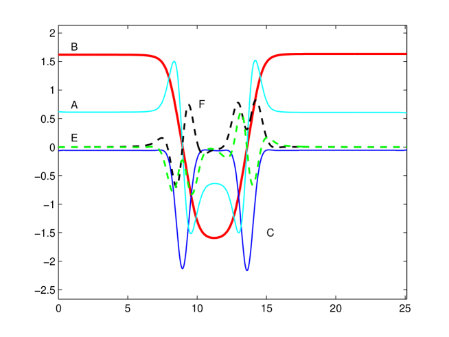
Figure 29: The vorticity field of the converged TW with $c=-3.22\times 10^{-3}$ and $\overline{F}=1.0241$ found from the DNS solution of figure 27. $F$ is the thickest (red) line, $\omega_{g}-Re/n$ is the thin (dark) blue line, $\omega_{h}$ the thin (light) cyan line, $\omega_{G}$ the dashed (light) green line and $\omega_{H}$ the dashed (dark) black line.

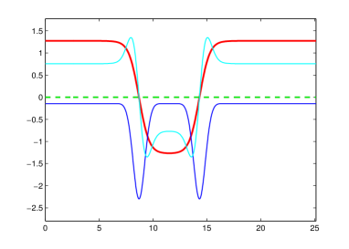
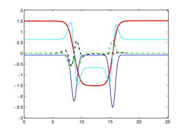
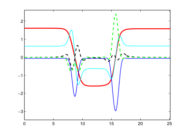
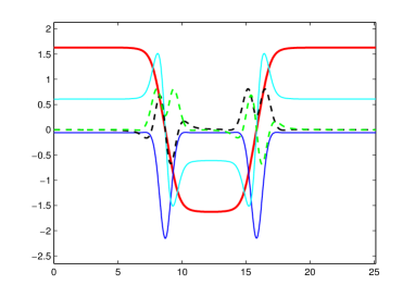
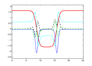
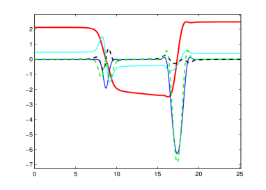
Figure 30: The vorticity fields of the solutions labelled $a$ (top left), $b$ (top right), $c$ (middle left), $d$ (middle right), $e$ (bottom left), $f$ (bottom right) in figure 31. In each, $F$ is the thickest (red) line, $\omega_{g}-Re/n$ is the thin (dark) blue line, $\omega_{h}$ the thin (light) cyan line, $\omega_{G}$ the dashed (light) green line and $\omega_{H}$ the dashed (dark) black line (as in figure 29). $\overline{F}=0.7055$ for all solutions.

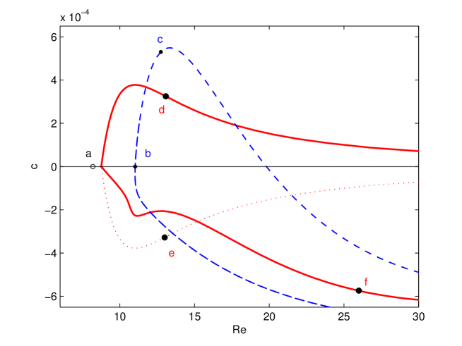
Figure 31: The travelling wave solution branches found in the 5-PDE system: similar branches with $c\rightarrow-c$ exist via symmetry transformations as, for example, has been shown for the upper solid red branch to produce the lower dotted branch. Plots of the vorticity fields at points labelled $a,b,c,d,e,f$ are given in figure 30. Solution $a$ is $\mathcal{S}-$ symmetric and so $c=0$. The thick red $\mathcal{S}-$ asymmetric branch crosses the $\mathcal{S}-$ symmetric branch at the asymmetric bifurcation point $Re\approx 8.75$ . Solution $b$ has $c=0$ but is not $\mathcal{S}-$ symmetric. Solutions $d$ and $e$ are complements of each other (same branch but opposite $c$). Solution $f$ shows the tendency for the kink pairs to separate and become unequal. $\overline{F}=0.7055$ for all solutions.

6 Discussion

The original motivation for this study was to look for an accessible arena in which to study spatiotemporal behaviour in the Navier-Stokes equation. Kolmogorov flow is by design a minimalist model of a viscous fluid flow being 2-dimensional, driven by a simple body force and subject to periodic boundary conditions in both directions. The results presented here indicate that despite this, it possesses rich spatiotemporal behaviour once larger domains are considered. Key to the observed dynamics is the existence of localised flow structures - kinks and antikinks - which, directly or indirectly through their bifurcated derivatives, appear to underpin all of the flow dynamics observed. The kinks and antikinks first arise during the initial long-wavelength instability away from the basic flow response which mirrors the forcing at low amplitudes. The structure of the ensuing state as a function of the forcing amplitude is described by a Cahn-Hilliard-type equation and quickly separates into two regions of roughly half the domain where a constant flow exists in either of the two directions perpendicular to the forcing. These regions are connected via kink and antikink transition regions and coarsening dynamics leading to this state are observed for random initial data.

After further bifurcations (typically modulational instabilities in $y$) as the forcing strengthens, this regime gives way to multiple attractors, some of which possess spatially-localised time dependence (P1 and P2). Co-existence of such attractors in a large domain gives rise to a variety of interesting collisional dynamics. A minimal 5-PDE (1-space and 1-time) system has been built by taking a 3-PDE improved long-wavelength approximation and incorporating the possibility of subharmonic instability. This extended system captures the behaviour seen and allows the basic building blocks of the behaviour - travelling waves - to be easily isolated. These consist of kink-antikink pairs whose phase speed and collisional behaviour depend on the separation between the kink and antikink and their internal vortical structures. At larger forcing amplitudes ($25\lesssim Re$ for a $8\pi\times 2\pi$ domain), the coarsening regime reinstates itself when various longest-wavelength solutions consisting of just one time-varying kink-antikink pair again become the only attractors. Beyond a yet higher forcing threshold ($120\lesssim Re$ for a $8\pi\times 2\pi$ domain), one longest-wavelength solution emerges as a unique attractor. In this, the kink and antikink are chaotic yet the two one-dimensional regions of essentially half the domain width remain steady.

The Cahn-Hilliard coarsening behaviour, demonstrated here in Kolmogorov flow for the first time, is not new but the exploration beyond this regime is for the 2D Navier-Stokes equations. Complementary work has been performed in simpler modelling equations (e.g Gelens & Knobloch (2011) in the complex Swift-Hohenberg equation and van Hecke et al. (1999) for coupled complex Ginzburg-Landau equations) and found similarly, if not more, complicated behaviour (e.g. see figure 11 of Gelens & Knobloch (2011)). Here we find no spontaneous sources or sinks of kinks and antikinks (van Hecke et al. (1999); Gelens & Knobloch (2011)) but instead conservation of both after collisions. Presumably the dynamics are smoother in 2D Kolmogorov flow because of the extra spatial dimension present rather than other differences like the character of the underlying instability (e.g. finite wavenumber and oscillatory in Gelens & Knobloch (2011) as opposed to vanishing wavenumber and steady here). Certainly, the presence of this extra dimension allows the kinks and antikinks to have various different internal distributions of vorticity which, along with the kink-antikink separation, determines how they move as a bound state. Gelens & Knobloch (2011) also report the existence of stable ‘breathing sinks’ (their figure 12(j)) which resemble the state P1 found here and other work by Beaume et al. (2011) focussing on the phenomenon of homoclinic snaking in 2D doubly diffusive convection has found localised chaos (their figure 13). While a complete mathematical rationale for the spatiotemporal behaviour found here is beyond the scope of the current work, we have at least identified a simpler 5-PDE system based upon a long wavelength limit and started to map out some of the kink-antikink travelling waves it possesses. Hopefully, this system can form the basis of further analysis. Perhaps the most important observation made here is that the coarsening regime seems to reinstate itself at large forcing amplitudes and eventually a global attractor emerges again dominated by the longest wavelength allowed by the system albeit with localised chaotic kink and antikink regions.

In terms of the original aim of this paper, 2D Kolmogorov flow has been shown to provide a rich environment to explore the existence of simple exact localised solutions to the 2D Navier-Stokes equations and to probe their relevance to the complicated flow dynamics seen using recurrent-flow analysis in the spirit of Chandler & Kerswell (2013). The disparity between the large domains used here and the spatial extent of the localised chaos which exists, however, highlights a key challenge: to develop efficient (practical) recurrent-flow analysis strategies which look for solutions only over sub-domains of the full simulated system. We hope to be able to report on progress soon.

Acknowledgements. We would like to thank Gary Chandler for advice on the numerical codes used here, to Basile Gallet for very helpful comments on an earlier version of the manuscript and to an anonymous referee who alerted us to relevant literature on direction-reversing travelling waves and helped us improve the presentation in many ways. We are also very grateful for numerous free days of GPU time on ‘Emerald’ (the e-Infrastructure South GPU supercomputer: http://www.einfrastructuresouth.ac.uk/cfi/emerald) and the support of EPSRC through grant EP/H010017/1.

Appendix: The long wavelength expansion

Providing $Re$ is close to $Re_{c}(\alpha)$, the unstable wavenumbers are $O(\sqrt{Re-Re_{c}(\alpha)})$ from the neutral curve opening the way up to a small wavenumber/long wavelength expansion in which $\partial_{x}\ll\partial_{y}$ (Nepomniashchii 1976, Chapman & Proctor 1980, Sivashinsky 1985). We just summarise this calculation here since the details (albeit with a different non-dimensionalisation ) are in Sivashinsky (1985) (Chapman & Proctor 1980 derived the same long wave equation but for convective cells in a nearly insulated liquid layer). We work with the streamfunction version of the governing equations (6)

$$\nabla^{2}\psi_{t}+\psi_{y}\nabla^{2}\psi_{x}-\psi_{x}\nabla^{2}\psi_{y}=\frac{1}{Re}\nabla^{4}\psi+n\cos(ny)$$ (25)

where subscripts indicate derivatives, $\omega=-\nabla^{2}\psi$, and $\epsilon\ll 1$ is defined by

$$\frac{1}{Re}=(1-\epsilon^{2})\frac{1}{Re_{c}}.$$ (26)

(here $Re_{c}$ without an argument means $Re_{c}(0)$). The appropriately rescaled space and time variables are $\tau=\epsilon^{4}t$, $X=\epsilon x$ and $Y=ny$. The streamfunction $\psi$ is expanded as $\psi=\psi^{0}+\epsilon\psi^{1}+\epsilon^{2}\psi^{2}+\epsilon^{3}\psi^{3}+\ldots$ and is crucially assumed to share the same spanwise periodicity as the forcing function, that is, $\psi$ is $2\pi$ periodic in $Y$ so it is $\mathcal{S}-$symmetric. This means that $\int^{2\pi}_{0}\,dY$ of 25 gives simply

$$\epsilon\int^{2\pi}_{0}\psi_{XX\tau}\,dY+n\int^{2\pi}_{0}(\psi_{Y}\psi_{XX})_{X}\,dY=\frac{\epsilon(1-\epsilon^{2})}{Re_{c}}\int^{2\pi}_{0}\psi_{XXXX}\,dY.$$ (27)

At $O(1)$, (25) becomes simply

$$\frac{n^{4}}{Re_{c}}\psi^{0}_{YYYY}+n\cos Y=0$$ (28)

with the solution

$$\psi^{0}=-Re_{c}/n^{3}\cos Y+A^{0}(X,\tau)$$ (29)

(the zeroth approximation of (27) is automatically satisfied). At $O(\epsilon)$, (25) requires the solution

$$\psi^{1}=\frac{Re_{c}^{2}}{n^{4}}A_{X}^{0}\sin Y+A^{1}(X,\tau)$$ (30)

with (27) giving $Re_{c}=\sqrt[4]{2}n^{3/2}$ at $O(\epsilon)$. At $O(\epsilon^{2})$, (25) requires

$$\psi^{2}=\frac{Re_{c}}{n}\biggl{(}-\frac{1}{n^{2}}\cos Y+(A_{X}^{0})^{2}\frac{Re_{c}^{2}}{n^{4}}\cos Y+\frac{Re_{c}}{n^{3}}A_{X}^{1}\sin Y\biggr{)}+A^{2}(X,\tau)$$ (31)

((27) at $O(\epsilon^{2})$ is automatically satisfied) and at $O(\epsilon^{3})$

$$\psi^{3} = \biggl{[}\frac{3Re_{c}^{2}}{n^{6}}A_{XXX}^{0}+\frac{2Re_{c}^{2}}{n^{4}}A_{X}^{0}-\frac{Re_{c}^{4}}{n^{6}}(A_{X}^{0})^{3}+\frac{Re_{c}^{2}}{n^{4}}A_{X}^{2}\biggr{]}\sin Y$$ (32)

$$\hskip 85.35826pt+\frac{2Re_{c}^{3}}{n^{6}}A_{X}^{0}A_{X}^{1}\cos Y+A^{3}(X,\tau).$$

The $O(\epsilon^{3})$ approximation to (27) then gives (after integrating immediately twice in $X$) the evolution equation for $A^{0}$:

$$A_{\tau}^{0}+\frac{3Re_{c}^{3}}{2n^{8}}A^{0}_{XXXX}+\frac{2Re_{c}^{3}}{n^{6}}A^{0}_{XX}-\frac{Re_{c}^{5}}{3n^{8}}(A_{X}^{0})_{X}^{3}=0.$$ (33)

where $Re_{c}^{2}=\sqrt{2}n^{3}$. This equation has a Lyapunov functional

$${\cal F}[A^{0}]:=\frac{Re^{3}_{c}}{12n^{8}}\int^{\epsilon L}_{0}\,\biggl{[}9(A^{0}_{XX})^{2}-12n^{2}(A^{0}_{X})^{2}+\sqrt{2}n^{3}(A^{0}_{X})^{4}\biggr{]}\,dX$$ (34)

such that

$$A^{0}_{\tau}=-\frac{\delta{\cal F}}{\delta A}.$$ (35)

As a result $d{\cal F}/{d\tau}=-\int^{\epsilon L}_{0}(A^{0}_{\tau})^{2}dX\leq 0$ and the dynamics is a monotonic approach to a local or global minimum of ${\cal F}$. Such a minimum satisfies

$$A^{0}_{XXX}+\frac{4n^{2}}{3}A^{0}_{X}-\frac{2\sqrt{2}n^{3}}{9}(A_{X}^{0})^{3}=\gamma.$$ (36)

where $\gamma$ is an integration constant. Multiplying by $A^{0}_{XX}$ and integrating again gives

$$\textstyle{1\over 2}(A^{0}_{XX})^{2}+\frac{2n^{2}}{3}(A^{0}_{X})^{2}-\frac{\sqrt{2}n^{3}}{18}(A_{X}^{0})^{4}-\gamma A^{0}_{X}=E.$$ (37)

with $E$ a further constant. As Chapman & Proctor (1980) point out, this equation represents a ‘particle’ with position $A_{X}^{0}$ oscillating spatially in a potential well

$$V(A^{0}_{X}):=\frac{2n^{2}}{3}(A^{0}_{X})^{2}-\frac{\sqrt{2}n^{3}}{18}(A_{X}^{0})^{4}-\gamma A^{0}_{X}$$ (38)

with total constant energy $E$. Since $A^{0}_{X}$ represents the (leading $O(\epsilon)$) spanwise velocity, it has zero mean,

$$\int^{\epsilon L}_{0}\,A^{0}_{X}\,dX\,=\,0,$$ (39)

which implies $\gamma=0$ otherwise the oscillation is not (spatially) centred on $A_{X}^{0}=0$. For a given domain length, there are then a countably infinite number of (spatially-) periodic solutions which fit into the domain although the wavelengths will eventually approach the width of the domain where the long-wavelength assumption breaks down. For solutions of the Euler-Lagrange equations (36) with $\gamma=0$, the integral relationship

$$\int^{\epsilon L}_{0}\,A^{0}_{X}(\ref{ELeqns})\,dX=\int^{\epsilon L}_{0}\frac{3}{2}(A^{0}_{XX})^{2}-2n^{2}(A^{0}_{X})^{2}+\frac{\sqrt{2}}{6}(A^{0}_{X})^{4}\,dX=0$$ (40)

can be used to simplify the stationary value of ${\cal F}$ to just

$${\cal F}_{stat}=-\frac{\sqrt{2}Re_{c}^{3}}{12n^{5}}\int^{\epsilon L}_{0}(A_{X}^{0})^{4}\,dX.$$ (41)

Unfortunately, this does not immediately indicate that the steady solution with longest wavelength is the global minimiser but stability analysis does indicate this (Nepomniashchii 1976, Chapman & Proctor 1980). All solutions of (36) are found to be unstable to perturbations of longer wavelength implying that the solution with longest possible wavelength will be the global attractor. This is borne out by simulations (e.g. She (1987)).

The solution to (36) (with $\gamma=0$) can be written down in terms of elliptic functions as

$$A_{X}^{0}=\sigma{\rm sn}(\beta X|k)$$ (42)

where, without loss of generality, $A_{X}^{0}(0)=0$ has been imposed,

$${\rm sn}(\beta X|k):=\sin\phi\quad{\rm where}\quad\beta X=\int^{\phi}_{0}\frac{d\theta}{\sqrt{1-k^{2}\sin^{2}\theta}},$$ (43)

and $\sigma,\beta$ and $k\in[0,1]$ are defined by the relations

$$(\beta\sigma)^{2}=2E,\quad\beta^{2}(1+k^{2})=\frac{4n^{2}}{3},\quad\frac{\beta^{2}}{\sigma^{2}}k^{2}=\frac{\sqrt{2}n^{3}}{9}.$$ (44)

There is one further relation which is the second boundary condition on $A_{X}^{0}$. Since $A_{X}^{0}$ is periodic over $\epsilon L=2\pi\epsilon/\alpha$, we can look for one cell over half the (spatial) period by setting $A^{0}_{X}=0$ at $X=\pi\epsilon/\alpha$ or equivalently $A^{0}_{XX}(\pi\epsilon/(2\alpha))=0$,

$$\frac{n\pi}{\sqrt{3(1+k^{2})}}\biggl{(}\frac{\epsilon}{\alpha}\biggr{)}=K(k):=\int^{\pi/2}_{0}\frac{d\theta}{\sqrt{1-k^{2}\sin^{2}\theta}}$$ (45)

where $K(k)$ is the complete elliptic integral of the first kind. This last condition defines $k\in[0,1]$ as a function of $\epsilon/\alpha$. The bifurcation point is approached as $k\rightarrow 0$ (which minimises $K(k)$) and yields the critical $\epsilon$ value as a function of the geometry

$$\epsilon_{crit}(\alpha):=\frac{\sqrt{3}\alpha}{2n}$$ (46)

which, when converted into a critical $Re$, is the result quoted in (13). In the other limit of $k\rightarrow 1$ corresponding to increasing $Re$ or a lengthening domain ($2\pi/\alpha$) or both,

$$\lim_{k\rightarrow 1}E=n\sqrt{2}=\max_{A^{0}_{X}}\,V(A_{X}^{0})$$ (47)

which is the maximum possible energy for a spatially oscillatory solution to (37) (with $\gamma=0$). In other words, there is no upper limit on $Re$ or $1/\alpha$ where such a solution no longer is available in this long-wave approximation. The solution simplifies in this $k\rightarrow 1$ limit to the localised solution

$$A_{X}^{0}=\sqrt{\frac{3\sqrt{2}}{n}}\tanh\biggl{(}n\sqrt{\frac{2}{3}}X\biggr{)}.$$ (48)

As $X=\pm\infty$, $A^{0}_{X}\rightarrow\pm\sqrt{3\sqrt{2}/n}$ so that the solution (48) acts to connect exact solutions of the form

$$\psi=\lambda x-\frac{Re}{n(Re^{2}\lambda^{2}+n^{2})}\cos(ny)+\frac{\lambda Re^{2}}{n^{2}(Re^{2}\lambda^{2}+n^{2})}\sin(ny)$$ (49)

where $\lambda=\epsilon\sqrt{3\sqrt{2}/n}$ represents the constant velocity component perpendicular to the forcing direction. In fact solutions (49) exist for all $\lambda$ but clearly only two states are viable asymptotic limits for $A_{X}^{0}$ (no net flow in the $y$ direction forces the two values to be equal in magnitude but opposite in sign).

References

- Alonso et al. (2000) Alonso, A, Sanchez, J & Net, M 2000 Transition to temporal chaos in an O(2)-symmetric convective system for low Prandtl numbers. Prog. Theor. Phys. Suppl. 139, 315–324.
- Armbruster et al. (1996) Armbruster, D, Nicolaenko, B, Smaoui, N & Chossat, Pascal 1996 Symmetries and dynamics for 2-D Navier-Stokes flow. Physica D: Nonlinear Phenomena 95 (1), 81–93.
- Arnol’d (1991) Arnol’d, V I 1991 Kolmogorov’s hydrodynamic attractors. Proc. R. Soc. Lond. A 434, 19–22.
- Arnold & Meshalkin (1960) Arnold, V I & Meshalkin, L D 1960 Seminar led by AN Kolmogorov on selected problems of analysis (1958-1959). Usp. Mat. Nauk 15 (247), 20–24.
- Avila et al. (2011) Avila, K, Moxey, D, de Lozar, A, Avila, M, Barkley, D & Hof, B 2011 The onset of turbulence in pipe flow. Science 333, 192–196.
- Balmforth & Young (2002) Balmforth, Neil J & Young, Yuan-Nan 2002 Stratified Kolmogorov flow. Journal of Fluid Mechanics 450, 131–168.
- Balmforth & Young (2005) Balmforth, Neil J & Young, Yuan-Nan 2005 Stratified Kolmogorov flow. Part 2. Journal of Fluid Mechanics 528 (1), 23–42.
- Batchaev (2012) Batchaev, A M 2012 Laboratory simulation of the Kolmogorov flow on a spherical surface. Izvestiya, Atmospheric and Oceanic Physics 48 (6), 657–662.
- Batchaev & Ponomarev (1989) Batchaev, A M & Ponomarev, V M 1989 Experimental and theoretical investigation of Kolmogorov flow on a cylindrical surface. Fluid Dynamics 24 (5), 675–680.
- Beaume et al. (2011) Beaume, C, Bergeon, A & Knobloch, E 2011 Homoclinic snaking of localized states in doubly diffusive convection. Phys. Fluids 23, 094102.
- Berti & Boffetta (2010) Berti, S & Boffetta, G 2010 Elastic waves and transition to elastic turbulence in a two-dimensional viscoelastic Kolmogorov flow. Physical Review E 82 (3), 036314.
- Boffetta et al. (2005) Boffetta, Guido, Celani, Antonio, Mazzino, Andrea, Puliafito, Alberto & Vergassola, Massimo 2005 The viscoelastic Kolmogorov flow: eddy viscosity and linear stability. Journal of Fluid Mechanics 523 (1), 161–170.
- Bondarenko et al. (1979) Bondarenko, N F, Gak, M Z & Dolzhanskii, F V 1979 Laboratory and theoretical models of plane periodic flow. Akademiia Nauk SSSR 15, 1017–1026.
- Borue & Orszag (2006) Borue, Vadim & Orszag, Steven A 2006 Numerical study of three-dimensional Kolmogorov flow at high Reynolds numbers. Journal of Fluid Mechanics 306 (-1), 293.
- Burgess et al. (1999) Burgess, John M, Bizon, C, McCormick, W D, Swift, J B & Swinney, Harry L 1999 Instability of the Kolmogorov flow in a soap film. Physical Review E 60 (1), 715.
- Chandler & Kerswell (2013) Chandler, Gary J & Kerswell, Rich R 2013 Invariant recurrent solutions embedded in a turbulent two-dimensional Kolmogorov flow. Journal of Fluid Mechanics 722, 554–595.
- Chapman & Proctor (1980) Chapman, C J & Proctor, MRE 1980 Nonlinear Rayleigh–Bénard convection between poorly conducting boundaries. Journal of Fluid Mechanics 101 (04), 759–782.
- Chen & Price (2004) Chen, Zhi-Min & Price, W G 2004 Chaotic behavior of a Galerkin model of a two-dimensional flow. Chaos: An Interdisciplinary Journal of Nonlinear Science 14 (4), 1056.
- Cvitanović & Gibson (2010) Cvitanović, P & Gibson, J F 2010 Geometry of the turbulence in wall-bounded shear flows: periodic orbits. Physica Scripta 142, 4007.
- Feudel & Seehafer (1995) Feudel, Fred & Seehafer, Norbert 1995 Bifurcations and pattern formation in a two-dimensional Navier-Stokes fluid. Physical Review E 52 (4), 3506.
- Fortova (2013) Fortova, S V 2013 Numerical simulation of the three-dimensional Kolmogorov flow in a shear layer. Computational Mathematics and Mathematical Physics 53 (3), 311–319.
- Fukuta & Murakami (1998) Fukuta, Hiroaki & Murakami, Youichi 1998 Side-wall effect on the long-wave instability in Kolmogorov flow. Journal of the Physical Society of Japan 67 (5), 1597–1602.
- Gallet & Young (2013) Gallet, Basile & Young, William R 2013 A two-dimensional vortex condensate at high Reynolds number. Journal of Fluid Mechanics 715, 359–388.
- Gelens & Knobloch (2011) Gelens, L & Knobloch, E 2011 Traveling waves and defects in the complex Swift-Hohenberg equation. Phys. Rev. E p. 056203.
- Gotoh & Yamada (1987) Gotoh, Kanefusa & Yamada, Michio 1987 The instability of rhombic cell flows. Fluid Dynamics Research 1 (3), 165–176.
- van Hecke et al. (1999) van Hecke, M, Storm, S & van Saarloos, W 1999 Sources, sinks and wavenumber selection in coupled CGL equations and experimental implications for counter-propagating wave systems. Physica D 134, 1–47.
- Kawahara & Kida (2001) Kawahara, Genta & Kida, Shigeo 2001 Periodic motion embedded in plane Couette turbulence: regeneration cycle and burst. Journal of Fluid Mechanics 449, 291.
- Kazantsev (1998) Kazantsev, Evgueni 1998 Unstable periodic orbits and attractor of the barotropic ocean model. Nonlinear processes in Geophysics 5 (4), 193–208.
- Kim & Okamoto (2003) Kim, S C & Okamoto, H 2003 Bifurcations and inviscid limit of rhombic Navier–Stokes flows in tori. IMA journal of applied mathematics 68 (2), 119–134.
- Kreilos & Eckhardt (2012) Kreilos, Tobias & Eckhardt, Bruno 2012 Periodic orbits near onset of chaos in plane Couette flow. Chaos: An Interdisciplinary Journal of Nonlinear Science 22 (4), 047505.
- Landsberg & Knobloch (1991) Landsberg, A S & Knobloch, E 1991 Direction-reversing travelling waves. Physics Lett. A 159, 17–20.
- Lorenz (1972) Lorenz, Edward N 1972 Barotropic Instability of Rossby Wave Motion. Journal of Atmospheric Sciences 29 (2), 258–265.
- Manela & Zhang (2012) Manela, A & Zhang, J 2012 The effect of compressibility on the stability of wall-bounded Kolmogorov flow. Journal of Fluid Mechanics 694, 29–49.
- Manfroi & Young (1999) Manfroi, A J & Young, W R 1999 Slow evolution of zonal jets on the beta plane. Journal of the Atmospheric Sciences 56 (5), 784–800.
- Marchioro (1986) Marchioro, C 1986 An example of absence of turbulence for any Reynolds number. Communications in Mathematical Physics 105 (1), 99–106.
- Meshalkin & Sinai (1961) Meshalkin, L D & Sinai, Y G 1961 Investigation of the stability of a stationary solution of a system of equations for the plane movement of an incompressible viscous liquid. Journal of Applied Mathematics and Mechanics 25, 1700–1705.
- Musacchio & Boffetta (2014) Musacchio, S & Boffetta, G 2014 Turbulent channel without boundaries: The periodic Kolmogorov flow. Phys. Rev. E 89, 023004.
- Nepomniashchii (1976) Nepomniashchii, A A 1976 On stability of secondary flows of a viscous fluid in unbounded space. Prikladnaia Matematika i Mekhanika 40, 886–891.
- Obukhov (1983) Obukhov, A M 1983 Kolmogorov flow and laboratory simulation of it. Russian Mathematical Surveys 38 (4), 113–126.
- Okamoto (1996) Okamoto, Hisashi 1996 Nearly singular two-dimensional kolmogorov flows for large reynolds numbers. Journal of Dynamics and Differential Equations 8 (2), 203–220.
- Okamoto (1998) Okamoto, Hisashi 1998 A study of bifurcation of Kolmogorov flows with an emphasis on the singular limit. Docum. Math., Proc. Int. Congress Math 3, 523–532.
- Okamoto & Shōji (1993) Okamoto, H & Shōji, M 1993 Bifurcation diagrams in Kolmogorov’s problem of viscous incompressible fluid on 2-D flat tori. Japan Journal of Industrial and Applied Mathematics 10 (2), 191–218.
- Platt et al. (1991) Platt, N, Sirovich, L & Fitzmaurice, N 1991 An investigation of chaotic Kolmogorov flows. Phys. Fluids A 3 (4), 681.
- Roeller et al. (2009) Roeller, Klaus, Vollmer, Jürgen & Herminghaus, Stephan 2009 Unstable Kolmogorov flow in granular matter. Chaos: An Interdisciplinary Journal of Nonlinear Science 19 (4), 041106.
- Rollin et al. (2011) Rollin, B, Dubief, Y & Doering, C R 2011 Variations on Kolmogorov flow: turbulent energy dissipation and mean flow profiles. Journal of Fluid Mechanics 670, 204–213.
- Sarris et al. (2007) Sarris, I E, Jeanmart, H, Carati, D & Winckelmans, G 2007 Box-size dependence and breaking of translational invariance in the velocity statistics computed from three-dimensional turbulent Kolmogorov flows. Physics of Fluids 19 (9), 095101.
- She (1987) She, Zhen Su 1987 Metastability and vortex pairing in the Kolmogorov flow. Physics Letters A 124 (3), 161–164.
- She (1988) She, Zhen Su 1988 Large-scale dynamics and transition to turbulence in the two-dimensional Kolmogorov flow. In IN: Current trends in turbulence research; Proceedings of the Fifth Beersheba International Seminar on Magnetohydrodynamics Flow and Turbulence, pp. 374–396. Nice, Observatoire, France.
- Shebalin & Woodruff (1997) Shebalin, John V & Woodruff, Stephen L 1997 Kolmogorov flow in three dimensions. Physics of Fluids 9 (1), 164.
- Sivashinsky (1985) Sivashinsky, Gregory I 1985 Weak turbulence in periodic flows. Physica D: Nonlinear Phenomena 17 (2), 243–255.
- Sommeria (1986) Sommeria, J 1986 Experimental study of the two-dimensional inverse energy cascade in a square box. Journal of Fluid Mechanics 170, 139–168.
- Suri et al. (2013) Suri, B, Tithof, J, Mitchell, Jr, R, Grigoriev, R O & F, Schatz M 2013 Velocity Profile in a Two-Layer Kolmogorov-Like Flow. arXiv:1307.6247v1 .
- Thess (1992) Thess, André 1992 Instabilities in two-dimensional spatially periodic flows. Part I: Kolmogorov flow. Phys. Fluids A 4 (7), 1385.
- Tsang & Young (2009) Tsang, Yue-Kin & Young, William 2009 Forced-dissipative two-dimensional turbulence: A scaling regime controlled by drag. Physical Review E 79 (4), 045308.
- Tsang & Young (2008) Tsang, Yue-Kin & Young, William R 2008 Energy-enstrophy stability of β-plane Kolmogorov flow with drag. Physics of Fluids 20 (8), 084102.
- van Veen et al. (2006) van Veen, Lennaert, Kida, Shigeo & Kawahara, Genta 2006 Periodic motion representing isotropic turbulence. Japan Society of Fluid Mechanics. Fluid Dynamics Research. An International Journal 38 (1), 19–46.
- Viswanath (2007) Viswanath, Divakar 2007 Recurrent motions within plane Couette turbulence. Journal of Fluid Mechanics 580, 339.
- Viswanath (2009) Viswanath, Divakar 2009 The critical layer in pipe flow at high Reynolds number. Philosophical Transactions of the Royal Society A: Mathematical, Physical and Engineering Sciences 367 (1888), 561–576.
- Willis et al. (2013) Willis, A P, Cvitanović, P & Avila, M 2013 Revealing the state space of turbulent pipe flow by symmetry reduction. Journal of Fluid Mechanics 721, 514–540.