Upper Bounds On the ML Decoding Error Probability of General Codes over AWGN Channels

Abstract

In this paper, parameterized Gallager’s first bounding technique (GFBT) is presented by introducing nested Gallager regions, to derive upper bounds on the ML decoding error probability of general codes over AWGN channels. The three well-known bounds, namely, the sphere bound (SB) of Herzberg and Poltyrev, the tangential bound (TB) of Berlekamp, and the tangential-sphere bound (TSB) of Poltyrev, are generalized to general codes without the properties of geometrical uniformity and equal energy. When applied to the binary linear codes, the three generalized bounds are reduced to the conventional ones. The new derivation also reveals that the SB of Herzberg and Poltyrev is equivalent to the SB of Kasami et al., which was rarely cited in the literatures.

I Introduction

In most scenarios, there do not exist easy ways to compute the exact decoding error probabilities for specific codes and ensembles. Therefore, deriving tight analytical bounds is an important research subject in the field of coding theory and practice. Since the early 1990s, spurred by the successes of the near-capacity-achieving codes, renewed attentions have been paid to the performance analysis of the maximum-likelihood (ML) decoding algorithm. Though the ML decoding algorithm is prohibitively complex for most practical codes, tight bounds can be used to predict their performance without resorting to computer simulations. As mentioned in [1], most bounding techniques have connections to either the 1965 Gallager bound [2, 3, 4, 5] or the 1961 Gallager bound [6, 7, 8, 9, 10, 11, 12, 13, 14, 15, 16, 17, 18] based on Gallager’s first bounding technique (GFBT). However, most previously reported upper bounds are focusing on binary linear codes.

For binary linear codes modulated by binary phase shift keying (BPSK), there are two main properties, which are geometrical uniformity and equal energy. The geometrical uniformity allows us to make an assumption that the all-zero codeword is the transmitted one, while the property of equal energy is critical to derive the tangential bound (TB) [6] and the tangential-sphere bound (TSB) [10]. For general codes without these two properties, performance analysis becomes more difficult than that for binary linear codes.

In this paper, we present parameterized GFBT by introducing nested Gallager regions to derive upper bounds on the ML decoding error probability of general codes over AWGN channels. The main contributions as well as the structure of this paper are summarized as follows.

1. We present in Sec. II the parameterized GFBT for general codes. We also present a necessary and sufficient condition on the optimal parameter, and a sufficient condition (with a simple geometrical explanation) under which the optimal parameter does not depend on the signal-to-noise ratio (SNR).

2. Within the general framework based on the introduced nested Gallager regions, three existing upper bounds, the sphere bound (SB) of Herzberg and Poltyrev [9], the tangential bound (TB) of Berlekamp [6] and the tangential-sphere bound (TSB) of Poltyrev [10], are generalized in Sec. III to general codes without the properties of geometrical uniformity and equal energy. The three upper bounds are then applied to binary linear codes and reduced to the conventional ones. The new derivation also reveals that the SB of Herzberg and Poltyrev is equivalent to the SB of Kasami et al. [7] [8], which was rarely cited in the literatures.

3. We use in Sec. IV terminated trellis codes [19] to illustrate how to calculate the parameterized Gallager first bounds on the frame-error probability. Numerical results are also presented in Sec. IV. Sec. V concludes this paper.

II The Parameterized Gallager’s First Bounds

II-A General Codes

A general code $\mathcal{C}(n,M)\subset\mathbb{R}^{n}$, in this paper, means a set that contains $M$ $n$-dimensional real vectors (referred to as codewords). The squared Euclidean distance between a codeword $\underline{s}$ and the origin point $\mathbb{O}$ of the $n$-dimensional space, denoted by $\|\underline{s}\|^{2}$, is also referred to as the energy of this codeword. If all codewords have the same energy, we say that the code has the property of equal energy.

Given a codeword $\underline{s}$, we denote $A_{\delta_{d}|\underline{s}}$ the number of codewords having the Euclidean distance $\delta_{d}$ with $\underline{s}$. We define

$$A_{\delta_{d}}\stackrel{{\scriptstyle\Delta}}{{=}}\sum_{\underline{s}}{\rm Pr}\{\underline{s}\}A_{\delta_{d}|\underline{s}},$$ (1)

which is the average number of ordered pairs of codewords with Euclidean distance $\delta_{d}$.

Definition 1

The Euclidean distance enumerating function of a general code $\mathcal{C}(n,M)$ is defined as

$$A(X)\stackrel{{\scriptstyle\Delta}}{{=}}\sum_{\delta_{d}}A_{\delta_{d}}X^{\delta_{d}^{2}},$$ (2)

where $X$ is a dummy variable and the summation is over all possible distance $\delta_{d}$. For a general code, there exist at most $\binom{M}{2}$ non-zero coefficients $\{A_{\delta_{d}}\}$, which is referred to as the Euclidean distance spectrum.

To derive tangential bounds, we also need another distance spectrum for general codes. Given a codeword $\underline{s}$ with energy $\delta_{d_{1}}^{2}$, we denote $B_{\delta_{d_{1}},\delta_{d_{2}},\delta_{d}|\underline{s}}$ the number of codewords $\underline{\hat{s}}$ having energy $\delta_{d_{2}}^{2}$ and the Euclidean distance $\delta_{d}$ with $\underline{s}$. We define

$$B_{\delta_{d_{1}},\delta_{d_{2}},\delta_{d}}\stackrel{{\scriptstyle\Delta}}{{=}}\sum_{\underline{s}}{\rm Pr}\{\underline{s}\}B_{\delta_{d_{1}},\delta_{d_{2}},\delta_{d}|\underline{s}},$$ (3)

which is the average number of ordered pairs of codewords with the Euclidean distance $\delta_{d}$ and energies $\delta_{d_{1}}^{2}$ and $\delta_{d_{2}}^{2}$, respectively.

Definition 2

The triangle Euclidean distance enumerating function of a general code $\mathcal{C}(n,M)$ is defined as

$$B(X,Y,Z)\stackrel{{\scriptstyle\Delta}}{{=}}\sum_{\delta_{d_{1}},\delta_{d_{2}},\delta_{d}}B_{\delta_{d_{1}},\delta_{d_{2}},\delta_{d}}X^{\delta_{d_{1}}^{2}}Y^{\delta_{d_{2}}^{2}}Z^{\delta_{d}^{2}},$$ (4)

where $X,Y,Z$ are three dummy variables. We call $\{B_{\delta_{d_{1}},\delta_{d_{2}},\delta_{d}}\}$ the triangle Euclidean distance spectrum of the given code.

II-B The Conventional Union Bound

Suppose that a codeword $\underline{s}=(s_{0},s_{1},\cdots,s_{n-1})\in\mathcal{C}(n,M)$ is transmitted over an AWGN channel. Let $\underline{y}={\underline{s}}+{\underline{z}}$ be the received vector, where $\underline{z}$ is a vector of independent Gaussian random variables with zero mean and variance $\sigma^{2}$. For AWGN channels, the maximum-likelihood (ML) decoding is equivalent to finding the nearest codeword $\hat{\underline{s}}$ to $\underline{y}$. The decoding error probability ${\rm Pr}\{E\}$ is

$${\rm Pr}\{E\}=\sum_{\underline{s}}{\rm Pr}\{\underline{s}\}{\rm Pr}\{E|\underline{s}\},$$ (5)

where ${\rm Pr}\{E|\underline{s}\}$ is the conditional decoding error probability when transmitting $\underline{s}$ over the channel. As usual, we assume that each codeword $\underline{s}$ is transmitted with equal probability, that is ${\rm Pr}\{\underline{s}\}=1/M$. With this assumption, the code rate is $\frac{\log M}{n}$ and the signal-to-noise ratio (SNR) is $\frac{\sum_{\underline{s}}\|\underline{s}\|^{2}}{nM\sigma^{2}}$.

The conventional union bound on the ML decoding error probability of a general code $\mathcal{C}(n,M)$ is

$${\rm Pr}\{E\} = \sum_{\underline{s}}{\rm Pr}\{\underline{s}\}{\rm Pr}\{E|\underline{s}\}$$ (6)

$$\leq \sum_{\underline{s}}{\rm Pr}\{\underline{s}\}\sum_{\delta_{d}}A_{\delta_{d}|\underline{s}}Q\left(\frac{\delta_{d}}{2\sigma}\right)$$

$$= \sum_{\delta_{d}}\sum_{\underline{s}}{\rm Pr}\{\underline{s}\}A_{\delta_{d}|\underline{s}}Q\left(\frac{\delta_{d}}{2\sigma}\right)$$

$$= \sum_{\delta_{d}}A_{\delta_{d}}Q\left(\frac{\delta_{d}}{2\sigma}\right),$$

where $Q\left(\frac{\delta_{d}}{2\sigma}\right)$ is the pair-wise error probability with

$$Q(x)\stackrel{{\scriptstyle\Delta}}{{=}}\int_{x}^{+\infty}\frac{1}{\sqrt{2\pi}}e^{-\frac{z^{2}}{2}}\,{\rm d}z.$$ (7)

The union bound is simple since it involves only the $Q$-function and does not require the code structure other than the Euclidean distance spectrum. However, the union bound is loose and even diverges in the low-SNR region. One way to solve this issue is to use the GFBT

$${\rm Pr}\{E|\underline{s}\}\leq{\rm Pr}\{E,\underline{y}\in\mathcal{R}|\underline{s}\}+{\rm Pr}\{\underline{y}\notin\mathcal{R}|\underline{s}\},$$ (8)

where $E$ denotes the conditional error event, $\underline{y}$ denotes the received signal vector, and $\mathcal{R}$ denotes an arbitrary region around the transmitted signal vector $\underline{s}$. The first term in the right hand side (RHS) of (8) is usually bounded by the conditional union bound, while the second term in the RHS of  (8) represents the probability of the event that the received vector $\underline{y}$ falls outside the region $\mathcal{R}$, which is considered to be decoded incorrectly even if it may not fall outside the Voronoi region [20] [21] of the transmitted codeword. For convenience, we call (8) $\mathcal{R}$-bound. Intuitively, the more similar the region $\mathcal{R}$ is to the Voronoi region of the transmitted signal vector, the tighter the $\mathcal{R}$-bound is. Therefore, both the shape and the size of the region $\mathcal{R}$ are critical to GFBT. Given the region’s shape, one can optimize its size to obtain the tightest $\mathcal{R}$-bound. Different from most existing works, where the size of $\mathcal{R}$ is optimized by setting to be zero the partial derivative of the bound with respect to a parameter (specifying the size), we will propose an alternative method by introducing nested Gallager’s regions in the subsection II-D.

II-C Binary Linear Codes

For a binary linear block code $\mathcal{C}(n,M)$ of dimension $k=\log_{2}M$, length $n$, and minimum Hamming distance $d_{\min}$, suppose that a codeword $\underline{c}$ is modulated by binary phase shift keying (BPSK), resulting in a bipolar signal vector $\underline{s}$ with $s_{t}=1-2c_{t}$ for $0\leq t\leq n-1$. Without loss of generality, we assume that the code $\mathcal{C}$ has at least three non-zero codewords, i.e., its dimension $k>1$, and the transmitted codeword is the all-zero codeword $\underline{c}^{(0)}$ (with bipolar image ${\underline{s}^{(0)}}$). Let ${\underline{\hat{c}}}$ (with bipolar image ${\underline{\hat{s}}}$) be a codeword of Hamming weight $d$, then the Euclidean distance between $\underline{s}^{(0)}$ and $\underline{\hat{s}}$ is $\delta_{d}=2\sqrt{d}$. We define

$$A_{d}\stackrel{{\scriptstyle\Delta}}{{=}}A_{\delta_{d}|\underline{s}^{(0)}},$$ (9)

which is the number of codewords with Hamming weight $d$. Since the constellation of binary linear block code is geometrically uniform and each codeword is assumed to be transmitted with equal probability, we have

$${\rm Pr}\{E\} = \sum_{\underline{s}}{\rm Pr}\{\underline{s}\}{\rm Pr}\{E|\underline{s}\}$$ (10)

$$= {\rm Pr}\{E|\underline{s}^{(0)}\}$$

$$\leq \sum_{d}A_{d}Q\left(\frac{\sqrt{d}}{\sigma}\right),$$

where $\{A_{d}\}$ is the weight distribution of the code $\mathcal{C}$.

II-D GFBT with Parameters

In this subsection, we will present parameterized GFBT by introducing nested Gallager regions with parameters so that Gallager bounds can be extended to general codes conveniently. To this end, let $\{\mathcal{R}(r),r\in\mathcal{I}\subseteq\mathbb{R}\}$ be a family of Gallager’s regions with the same shape and parameterized by $r\in\mathcal{I}$. For example, the nested regions can be chosen as a family of $n$-dimensional spheres of radius $r\geq 0$ centered at the transmitted codeword ${\underline{s}}$. We make the following assumptions.

Assumptions.

1. The regions $\{\mathcal{R}(r),r\in\mathcal{I}\subseteq\mathbb{R}\}$ are nested and their boundaries partition the whole space $\mathbb{R}^{n}$. That is,

   $$\mathcal{R}(r_{1})\subset\mathcal{R}(r_{2})~{}{\rm if}~{}r_{1}<r_{2},$$ (11)

   $$\partial\mathcal{R}(r_{1})\bigcap\partial\mathcal{R}(r_{2})=\emptyset~{}{\rm if}~{}r_{1}\neq r_{2},$$ (12)

   and

   $$\mathbb{R}^{n}=\bigcup\limits_{r\in\mathcal{I}}\partial\mathcal{R}(r),$$ (13)

   where $\partial\mathcal{R}(r)$ denotes the boundary surface of the region $\mathcal{R}(r)$.

2. Define a functional $R:{\underline{y}}\mapsto r$ whenever ${\underline{y}}\in\partial\mathcal{R}(r)$. The randomness of the received vector $\underline{y}$ then induces a random variable $R$. We assume that $R$ has a probability density function (pdf) $g(r)$.

3. We also assume that ${\rm Pr}\{E|{\underline{y}}\in\partial\mathcal{R}(r),\underline{s}\}$ can be upper-bounded by a computable upper bound $f_{u}(r|\underline{s})$.

For ease of notation, we may enlarge the index set $\mathcal{I}$ to $\mathbb{R}$ by setting $g(r)\equiv 0$ for $r\notin\mathcal{I}$. Under the above assumptions, we have the following parameterized GFBT .

Proposition 1

For any $r^{*}\in\mathbb{R}$,

$${\rm Pr}\{E|\underline{s}\}\leq\int_{-\infty}^{r^{*}}f_{u}(r|\underline{s})g(r)~{}{\rm d}r+\int_{r^{*}}^{+\infty}g(r)~{}{\rm d}r.$$ (14)

Proof:

$${\rm Pr}\{E|\underline{s}\} = {\rm Pr}\{E,\underline{y}\in\mathcal{R}(r^{*})|\underline{s}\}+{\rm Pr}\{E,\underline{y}\notin\mathcal{R}(r^{*})|\underline{s}\}$$

$$\leq {\rm Pr}\{E,\underline{y}\in\mathcal{R}(r^{*})|\underline{s}\}+{\rm Pr}\{\underline{y}\notin\mathcal{R}(r^{*})|\underline{s}\}$$

$$\leq \int_{-\infty}^{r^{*}}f_{u}(r|\underline{s})g(r)~{}{\rm d}r+\int_{r^{*}}^{+\infty}g(r)~{}{\rm d}r.$$

∎

An immediate question is how to choose $r^{*}$ to make the above bound as tight as possible? A natural method is to set the derivative of (14) with respect to $r^{*}$ to be zero and then solve the equation. In this paper, we propose an alternative method for gaining insight into the optimal parameter.

Before presenting a necessary and sufficient condition on the optimal parameter, we need emphasize that the computable bound $f_{u}(r|\underline{s})$ may exceed one. We also assume that $f_{u}(r|\underline{s})$ is non-trivial, i.e., there exists some $r$ such that $f_{u}(r|\underline{s})\leq 1$. For example, $f_{u}(r|\underline{s})$ can be taken as the union bound conditional on ${\underline{y}}\in\partial\mathcal{R}(r)$.

Theorem 1

Assume that $f_{u}(r|\underline{s})$ is a non-decreasing and continuous function of $r$. Let $r_{1}$ be a parameter that minimizes the upper bound as shown in (14). Then $r_{1}=\sup\{r\in\mathcal{I}\}$ if $f_{u}(r|\underline{s})<1$ for all $r\in\mathcal{I}$; otherwise, $r_{1}$ can be taken as any solution of $f_{u}(r|\underline{s})=1$. Furthermore, if $f_{u}(r|\underline{s})$ is strictly increasing in an interval $[r_{\min},r_{\max}]$ such that $f_{u}(r_{\min}|\underline{s})<1$ and $f_{u}(r_{\max}|\underline{s})>1$, there exists a unique $r_{1}\in[r_{\min},r_{\max}]$ such that $f_{u}(r_{1}|\underline{s})=1$.

Proof:

The second part is obvious since the function $f_{u}(r|\underline{s})$ is strictly increasing and continuous, which is helpful for solving numerically the equation $f_{u}(r|\underline{s})=1$.

To prove the first part, it suffices to prove that neither $r_{0}<\sup\{r\in\mathcal{I}\}$ with $f_{u}(r_{0}|\underline{s})<1$ nor $r_{2}$ with $f_{u}(r_{2}|\underline{s})>1$ can be optimal.

Let $r_{0}<\sup\{r\in\mathcal{I}\}$ such that $f_{u}(r_{0}|\underline{s})<1$. Since $f_{u}(r|\underline{s})$ is continuous and $r_{0}<\sup\{r\in\mathcal{I}\}$, we can find $\mathcal{I}\ni r^{\prime}>r_{0}$ such that $f_{u}(r^{\prime}|\underline{s})<1$. Then we have

$$\int_{-\infty}^{r_{0}}f_{u}(r|\underline{s})g(r)~{}{\rm d}r+\int_{r_{0}}^{+\infty}g(r)~{}{\rm d}r$$

$$= \int_{-\infty}^{r_{0}}f_{u}(r|\underline{s})g(r)~{}{\rm d}r+\int_{r_{0}}^{r^{\prime}}g(r)~{}{\rm d}r+\int_{r^{\prime}}^{+\infty}g(r)~{}{\rm d}r$$

$$> \int_{-\infty}^{r_{0}}f_{u}(r|\underline{s})g(r)~{}{\rm d}r+\int_{r_{0}}^{r^{\prime}}f_{u}(r|\underline{s})g(r)~{}{\rm d}r+\int_{r^{\prime}}^{+\infty}g(r)~{}{\rm d}r$$

$$= \int_{-\infty}^{r^{\prime}}f_{u}(r|\underline{s})g(r)~{}{\rm d}r+\int_{r^{\prime}}^{+\infty}g(r)~{}{\rm d}r,$$

where we have used the fact that $f_{u}(r|\underline{s})<1$ for $r\in[r_{0},r^{\prime}]$. This shows that $r^{\prime}$ is better than $r_{0}$.

Suppose that $r_{2}$ is a parameter such that $f_{u}(r_{2}|\underline{s})>1$. Since $f_{u}(r|\underline{s})$ is continuous and non-trivial, we can find $r_{1}<r_{2}$ such that $f_{u}(r_{1}|\underline{s})=1$. Then we have

$$\int_{-\infty}^{r_{2}}f_{u}(r|\underline{s})g(r)~{}{\rm d}r+\int_{r_{2}}^{+\infty}g(r)~{}{\rm d}r$$

$$= \int_{-\infty}^{r_{1}}f_{u}(r|\underline{s})g(r)~{}{\rm d}r+\int_{r_{1}}^{r_{2}}f_{u}(r|\underline{s})g(r)~{}{\rm d}r+\int_{r_{2}}^{+\infty}g(r)~{}{\rm d}r$$

$$> \int_{-\infty}^{r_{1}}f_{u}(r|\underline{s})g(r)~{}{\rm d}r+\int_{r_{1}}^{r_{2}}g(r)~{}{\rm d}r+\int_{r_{2}}^{+\infty}g(r)~{}{\rm d}r$$

$$= \int_{-\infty}^{r_{1}}f_{u}(r|\underline{s})g(r)~{}{\rm d}r+\int_{r_{1}}^{+\infty}g(r)~{}{\rm d}r,$$

where we have used a condition that $f_{u}(r|\underline{s})>1$ for $r\in(r_{1},r_{2}]$, which can be fulfilled by choosing $r_{1}$ to be the maximum solution of $f_{u}(r|\underline{s})=1$. This shows that $r_{1}$ is better than $r_{2}$. ∎

Corollary 1

Let $f_{u}(r|\underline{s})$ be a non-decreasing and continuous function of $r$. If $f_{u}(r|\underline{s})$ does not depend on the SNR, then the optimal parameter $r_{1}$ minimizing the upper bound (14) does not depend on the SNR, either.

Proof:

It is an immediate result from Theorem 1. ∎

Theorem 1 requires $f_{u}(r|\underline{s})$ to be a non-decreasing and continuous function of $r$, which can be fulfilled for several well-known bounds. Without such a condition, we may use the following more general theorem.

Theorem 2

For any measurable subset $\mathcal{A}\subset\mathcal{I}$, we have

$${\rm Pr}\{E|\underline{s}\}\leq\int_{r\in\mathcal{A}}f_{u}(r|\underline{s})g(r)~{}{\rm d}r+\int_{r\notin\mathcal{A}}g(r)~{}{\rm d}r.$$ (15)

Within this type, the tightest bound is

$${\rm Pr}\{E|\underline{s}\}\leq\int_{r\in\mathcal{I}_{0}}f_{u}(r|\underline{s})g(r)~{}{\rm d}r+\int_{r\notin\mathcal{I}_{0}}g(r)~{}{\rm d}r,$$ (16)

where $\mathcal{I}_{0}=\{r\in\mathcal{I}|f_{u}(r|\underline{s})<1\}$. Equivalently, we have

$${\rm Pr}\{E|\underline{s}\}\leq\int_{r\in\mathcal{I}}\min\{f_{u}(r|\underline{s}),1\}g(r)~{}{\rm d}r.$$ (17)

Proof:

Let $\mathcal{G}=\bigcup_{r\in\mathcal{A}}\partial\mathcal{R}(r)$, we have

$${\rm Pr}\{E|\underline{s}\} \leq {\rm Pr}\{E,{\underline{y}}\in\mathcal{G}|\underline{s}\}+{\rm Pr}\{{\underline{y}}\notin\mathcal{G}|\underline{s}\}$$

$$= \int_{r\in\mathcal{A}}f_{u}(r|\underline{s})g(r)~{}{\rm d}r+\int_{r\notin\mathcal{A}}g(r)~{}{\rm d}r.$$

Define $\mathcal{A}_{0}=\{r\in\mathcal{A}|f_{u}(r|\underline{s})<1\}$ and $\mathcal{A}_{1}=\{r\in\mathcal{A}|f_{u}(r|\underline{s})\geq 1\}$. Similarly, define $\mathcal{B}_{0}=\{r\notin\mathcal{A}|f_{u}(r|\underline{s})<1\}$ and $\mathcal{B}_{1}=\{r\notin\mathcal{A}|f_{u}(r|\underline{s})\geq 1\}$. Noticing that

$$\int_{r\in\mathcal{A}}\!\!f_{u}(r|\underline{s})g(r)~{}{\rm d}r\!\!\! \geq \!\!\!\int_{r\in\mathcal{A}_{0}}\!\!f_{u}(r|\underline{s})g(r)~{}{\rm d}r+\int_{r\in\mathcal{A}_{1}}\!\!g(r)~{}{\rm d}r$$

$$\int_{r\notin\mathcal{A}}\!\!g(r)~{}{\rm d}r\!\!\! \geq \!\!\!\int_{r\in\mathcal{B}_{0}}\!\!f_{u}(r|\underline{s})g(r)~{}{\rm d}r+\int_{r\in\mathcal{B}_{1}}\!\!g(r)~{}{\rm d}r,$$

we have

$$\int_{r\in\mathcal{A}}f_{u}(r|\underline{s})g(r)~{}{\rm d}r+\int_{r\notin\mathcal{A}}g(r)~{}{\rm d}r$$

$$\geq \int_{r\in\mathcal{A}_{0}\bigcup\mathcal{B}_{0}}f_{u}(r|\underline{s})g(r)~{}{\rm d}r+\int_{r\in\mathcal{A}_{1}\bigcup\mathcal{B}_{1}}g(r)~{}{\rm d}r$$

$$= \int_{r\in\mathcal{I}_{0}}f_{u}(r|\underline{s})g(r)~{}{\rm d}r+\int_{r\notin\mathcal{I}_{0}}g(r)~{}{\rm d}r$$

$$= \int_{r\in\mathcal{I}}\min\{f_{u}(r|\underline{s}),1\}g(r)~{}{\rm d}r.$$

∎

II-E Conditional Pair-Wise Error Probabilities

Let $\delta_{d}$ denote the Euclidean distance between $\underline{s}$ (the transmitted codeword) and a codeword $\underline{\hat{s}}$. The pair-wise error probability conditional on the event $\{{\underline{y}}\in\partial\mathcal{R}(r)\}$, denoted by $p_{2}(r,\delta_{d})$, is

$$p_{2}(r,\delta_{d}) = {\rm Pr}\left\{\|\underline{y}-\underline{\hat{s}}\|\leq\|\underline{y}-\underline{s}\|\mid\underline{y}\in\partial\mathcal{R}(r)\right\}$$ (18)

$$= \frac{\int_{\|\underline{y}-\underline{\hat{s}}\|\leq\|\underline{y}-\underline{s}\|,~{}~{}\underline{y}\in\partial\mathcal{R}(r)}f(\underline{y})~{}{\rm d}{\underline{y}}}{\int_{\underline{y}\in\partial\mathcal{R}(r)}f(\underline{y})~{}{\rm d}{\underline{y}}},$$

where $f({\underline{y}})$ is the pdf of $\underline{y}$. Noticing that, different from the unconditional pair-wise error probabilities, $p_{2}(r,\delta_{d})$ may be zero for some $r$.

We have the following lemma.

Lemma 1

Suppose that, conditional on $\underline{y}\in\partial\mathcal{R}(r)$, the received vector $\underline{y}$ is uniformly distributed over $\partial\mathcal{R}(r)$. Then the conditional pair-wise error probability $p_{2}(r,\delta_{d})$ does not depend on the SNR.

Proof:

Since $f(\underline{y})$ is constant for ${\underline{y}}\in\partial\mathcal{R}(r)$, we have, by canceling $f(\underline{y})$ from both the numerator and the denominator of $(\ref{Cpairwise})$,

$$p_{2}(r,\delta_{d})=\frac{\int_{\|\underline{y}-\underline{\hat{s}}\|\leq\|\underline{y}-\underline{s}\|,\underline{y}\in\partial\mathcal{R}(r)}~{}{\rm d}{\underline{y}}}{\int_{\underline{y}\in\partial\mathcal{R}(r)}~{}{\rm d}{\underline{y}}},$$ (19)

which shows that the conditional pair-wise error probability can be represented as a ratio of two “surface area” and hence does not depend on the SNR. ∎

Theorem 3

Let $f_{u}(r|\underline{s})$ be the conditional union bound, that is,

$$f_{u}(r|\underline{s})=\sum_{\delta_{d}}A_{\delta_{d}|\underline{s}}p_{2}(r,\delta_{d}).$$ (20)

Suppose that, conditional on $\underline{y}\in\partial\mathcal{R}(r)$, the received vector $\underline{y}$ is uniformly distributed over $\partial\mathcal{R}(r)$. If $f_{u}(r|\underline{s})$ is a non-decreasing and continuous function of $r$, then the optimal parameter $r_{1}$ minimizing the bound (14) does not depend on SNR but only on the distance spectrum of the code.

Proof:

From Lemma 1, we know that $f_{u}(r|\underline{s})$ does not depend on the SNR. From Corollary 1, we know that $r_{1}$ does not depend on the SNR.

More generally, without the condition that $f_{u}(r|\underline{s})$ is a non-decreasing and continuous function of $r$, the optimal interval $\mathcal{I}_{0}$ defined in Theorem 2 does not depend on the SNR, either.

∎

II-F General Framework of Parameterized GFBT

From the above subsection, we can see that there are three main steps to derive a parameterized GFBT. First, choose properly nested regions specified by a parameter. Second, find the pdf of the parameter. Finally, find a computable upper bound on the conditional decoding error probability given that the received vector falls on the boundary of a parameter-specified region. The key of the third step is to find the “projection” of the codewords to the boundary. Here, the “projection” means that the intersection between the perpendicular bisector of the segment $\overline{\underline{s}\ \underline{\hat{s}}}$ ($\underline{s}$ and $\underline{\hat{s}}$ are the transmitted codeword and decoded codeword, respectively) and the boundary.

III Single-Parameterized Upper Bounds for General Codes

For a general code, the property of geometrical uniformity may not hold. As a result, we can not assume a particular transmitted codeword and must average over all conditional error probabilities. In this section, we will first derive the conditional upper bound of ${\rm Pr}\{E|\underline{s}\}$ when transmitting the codeword $\underline{s}$ over the channel according to the framework of the parameterized GFBT, and then obtain the upper bound of ${\rm Pr}\{E\}$ from (5).

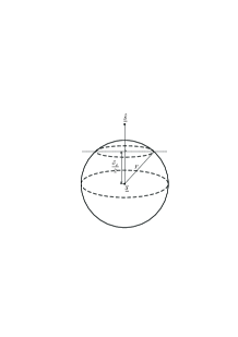
Figure 1: The geometric interpretation of the SB for general codes.

III-A The Parameterized Sphere Bound

III-A1 Nested Regions

The parameterized SB chooses the nested regions to be a family of $n$-dimensional spheres centered at the transmitted signal vector $\underline{s}$, that is, $\mathcal{R}(r)=\{\underline{y}\mid\|\underline{y}-\underline{s}\|\leq r\}$, where $r\geq 0$ is the parameter. See Fig. 1 for reference.

III-A2 Probability Density Function of the Parameter

The pdf of the parameter is

$$g(r)=\frac{2r^{n-1}e^{-\frac{r^{2}}{2\sigma^{2}}}}{2^{\frac{n}{2}}\sigma^{n}\Gamma(\frac{n}{2})},~{}~{}r\geq 0.$$ (21)

III-A3 Conditional Upper Bound

The parameterized SB chooses $f_{u}(r|\underline{s})$ to be the conditional union bound when transmitting the codeword $\underline{s}$ over the channel. Given that $||{\underline{y}}-{\underline{s}}||=r$, $\underline{y}$ is uniformly distributed over $\partial\mathcal{R}(r)$. Hence the conditional pair-wise error probability $p_{2}(r,\delta_{d})$ does not depend on the SNR and can be evaluated as the ratio of the surface area of a spherical cap to that of the whole sphere. That is,

$$\!\!\!\!\!p_{2}(r,\delta_{d})\!\!=\!\!\left\{\begin{array}[]{rl}\frac{\Gamma(\frac{n}{2})}{\sqrt{\pi}~{}\Gamma(\frac{n-1}{2})}\int_{0}^{\arccos(\frac{\delta_{d}}{2r})}\sin^{n-2}\phi~{}{\rm d}\phi,&r>\frac{\delta_{d}}{2}\\ 0,&r\leq\frac{\delta_{d}}{2}\end{array}\right..$$ (22)

Then the conditional union bound is given by

$$f_{u}(r|\underline{s})=\sum_{\delta_{d}}A_{\delta_{d}|\underline{s}}p_{2}(r,\delta_{d}).$$ (23)

III-A4 The Parameterized SB

From (17), we have

$${\rm Pr}\{E|\underline{s}\}\leq\int_{0}^{+\infty}\min\{f_{u}(r|\underline{s}),1\}g(r)~{}{\rm d}r.$$ (24)

From (1), we define

$$f_{u}(r) \triangleq \sum_{\underline{s}}{\rm Pr}\{\underline{s}\}f_{u}(r|\underline{s})$$ (25)

$$= \sum_{\underline{s}}{\rm Pr}\{\underline{s}\}\sum_{\delta_{d}}A_{\delta_{d}|\underline{s}}p_{2}(r,\delta_{d})$$

$$= \sum_{\delta_{d}}\sum_{\underline{s}}{\rm Pr}\{\underline{s}\}A_{\delta_{d}|\underline{s}}p_{2}(r,\delta_{d})$$

$$= \sum_{\delta_{d}}A_{\delta_{d}}p_{2}(r,\delta_{d}).$$

From (5), the parameterized SB for general codes can be written as

$${\rm Pr}\{E\} = \sum_{\underline{s}}{\rm Pr}\{\underline{s}\}{\rm Pr}\{E|\underline{s}\}$$ (26)

$$\leq \sum_{\underline{s}}{\rm Pr}\{\underline{s}\}\int_{0}^{+\infty}\min\left\{f_{u}(r|\underline{s}),1\right\}g(r)~{}{\rm d}r$$

$$\leq \int_{0}^{+\infty}\min\left\{\sum_{\underline{s}}{\rm Pr}\{\underline{s}\}f_{u}(r|\underline{s}),1\right\}g(r)~{}{\rm d}r$$

$$= \int_{0}^{+\infty}\min\left\{f_{u}(r),1\right\}g(r)~{}{\rm d}r,$$

which is determined by the Euclidean distance spectrum $\{A_{\delta_{d}}\}$.

III-A5 Reduction to Binary Linear Codes

For binary linear codes, the transmitted codeword $\underline{s}$ can be assumed to be the all-zero codeword $\underline{s}^{(0)}$. The Euclidean distance between a codeword $\underline{\hat{s}}$ with Hamming weight $d$ and $\underline{s}^{(0)}$ is $\delta_{d}=2\sqrt{d}$. Therefore, from (9), (22) and (23), the conditional union bound $f_{u}(r|\underline{s}^{(0)})$ can be written as

$$f_{u}(r|\underline{s}^{(0)}) = \sum_{\delta_{d}}A_{\delta_{d}|\underline{s}^{(0)}}p_{2}(r,\delta_{d})$$ (27)

$$= \sum_{1\leq d\leq n}A_{d}p_{2}(r,d),$$

where

$$\!\!\!\!\!p_{2}(r,d)\!\!=\!\!\left\{\begin{array}[]{rl}\frac{\Gamma(\frac{n}{2})}{\sqrt{\pi}~{}\Gamma(\frac{n-1}{2})}\int_{0}^{\arccos(\frac{\sqrt{d}}{r})}\sin^{n-2}\phi~{}{\rm d}\phi,&r>\sqrt{d}\\ 0,&r\leq\sqrt{d}\end{array}\right.,$$ (28)

which is a non-decreasing and continuous function of $r$ such that $p_{2}(0,d)=0$ and $p_{2}(+\infty,d)=1/2$. Therefore,

$$f_{u}(r) = \sum_{\underline{s}}{\rm Pr}\{\underline{s}\}f_{u}(r|\underline{s})$$ (29)

$$= f_{u}(r|\underline{s}^{(0)})$$

$$= \sum_{1\leq d\leq n}A_{d}p_{2}(r,d)$$

is also a non-decreasing and continuous function of $r$ such that $f_{u}(0)=0$ and $f_{u}(+\infty)\geq 3/2$. Furthermore, $f_{u}(r)$ is a strictly increasing function in the interval $[\sqrt{d_{\min}},+\infty)$ with $f_{u}(\sqrt{d_{\min}})=0$. Hence there exists a unique $r_{1}$ satisfying

$$\sum_{1\leq d\leq n}A_{d}p_{2}(r,d)=1,$$ (30)

which is equivalent to that given in [1, (3.48)] by noticing that $p_{2}(r,d)=0$ for $d>r^{2}$.

The parameterized SB for binary linear codes can be written as

$${\rm Pr}\{E\} \leq \int_{0}^{r_{1}}f_{u}(r)g(r)~{}{\rm d}r+\int_{r_{1}}^{+\infty}g(r)~{}{\rm d}r$$ (31)

$$= \int_{0}^{+\infty}\min\{f_{u}(r),1\}g(r)~{}{\rm d}r,$$

where $g(r)$ and $f_{u}(r)$ are given in (21) and (29), respectively. The optimal parameter $r_{1}$ is given by solving the equation (30), which does not depend on the SNR. It can be seen that (31) is exactly the sphere bound of Kasami et al [7][8]. It can also be proved that (31) is equivalent to that given in [1, (3.45)-(3.48)]. Firstly, we have shown that the optimal radius $r_{1}$ satisfies (30), which is equivalent to that given in [1, (3.48)]. Secondly, by changing variables, $z_{1}=r\cos\phi$ and $y=r^{2}$, it can be verified that (31) is equivalent to that given in [1, Sec.3.2.5].

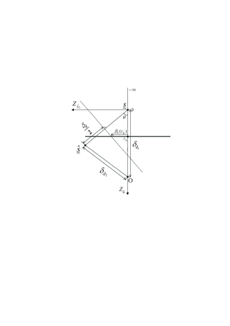
Figure 2: The geometric interpretation of the TB and TSB for general codes.

III-B The Parameterized Tangential Bound

In the derivation of the TB and TSB for binary codes, the equal-energy property plays a critical role. In the rest of this section, we show that the framework of the parameterized GFBT helps us to generalize the TB and TSB to general codes without the equal-energy property.

The AWGN sample $\underline{z}$ can be separated by projection as a radial component $z_{\xi_{1}}$ and $n-1$ tangential (orthogonal) components $\{z_{\xi_{i}},2\leq i\leq n\}$. Specifically, we set $z_{\xi_{1}}$ to be the inner product of $\underline{z}$ and $-{\underline{s}}/\delta_{d_{1}}$, where $\delta_{d_{1}}^{2}$ is the energy of $\underline{s}$. When considering the pair-wise error probability, we assume that $z_{\xi_{2}}$ is the component that lies in the plane determined by ${\underline{s}}$ and $\underline{\hat{s}}$. See Fig. 2 for reference.

III-B1 Nested Regions

The parameterized TB chooses the nested regions to be a family of half-spaces $Z_{\xi_{1}}\leq z_{\xi_{1}}$, where $z_{\xi_{1}}\in\mathbb{R}$ is the parameter. See Fig. 2 for reference.

III-B2 Probability Density Function of the Parameter

The pdf of the parameter is

$$g(z_{\xi_{1}})=\frac{1}{\sqrt{2\pi}\sigma}e^{-\frac{z_{\xi_{1}}^{2}}{2\sigma^{2}}}.$$ (32)

III-B3 Conditional Upper Bound

The parameterized TB chooses $f_{u}(z_{\xi_{1}}|\underline{s})$ to be the conditional union bound when transmitting the codeword $\underline{s}$ over the channel. Given that $Z_{\xi_{1}}=z_{\xi_{1}}$, the conditional pair-wise error probability is given by

$$p_{2}(z_{\xi_{1}},\delta_{d_{1}},\delta_{d_{2}},\delta_{d})=\int_{\beta_{d}(z_{\xi_{1}})}^{+\infty}\frac{1}{\sqrt{2\pi}\sigma}e^{-\frac{z_{\xi_{2}}^{2}}{2\sigma^{2}}}~{}{\rm d}z_{\xi_{2}},$$ (33)

where

$$\beta_{d}(z_{\xi_{1}})=\frac{\delta_{d}-2z_{\xi_{1}}\cos{\theta}}{2\sin{\theta}},$$ (34)

and

$$\theta=\arccos\left(\frac{\delta_{d_{1}}^{2}+\delta_{d}^{2}-\delta_{d_{2}}^{2}}{2\delta_{d_{1}}\delta_{d}}\right).$$ (35)

Then the conditional union bound is given by

$$f_{u}(z_{\xi_{1}}|\underline{s})=\sum_{\delta_{d_{1}},\delta_{d_{2}},\delta_{d}}B_{\delta_{d_{1}},\delta_{d_{2}},\delta_{d}|\underline{s}}p_{2}(z_{\xi_{1}},\delta_{d_{1}},\delta_{d_{2}},\delta_{d}).$$ (36)

III-B4 The Parameterized TB

From (17), we have

$${\rm Pr}\{E|\underline{s}\}\leq\int_{-\infty}^{+\infty}\min\{f_{u}(z_{\xi_{1}}|\underline{s}),1\}g(z_{\xi_{1}})~{}{\rm d}z_{\xi_{1}}.$$ (37)

From (3), we define

$$f_{u}(z_{\xi_{1}}) \triangleq \sum_{\underline{s}}{\rm Pr}\{\underline{s}\}f_{u}(z_{\xi_{1}}|\underline{s})$$ (38)

$$= \sum_{\underline{s}}{\rm Pr}\{\underline{s}\}\sum_{\delta_{d_{1}},\delta_{d_{2}},\delta_{d}}B_{\delta_{d_{1}},\delta_{d_{2}},\delta_{d}|\underline{s}}p_{2}(z_{\xi_{1}},\delta_{d_{1}},\delta_{d_{2}},\delta_{d})$$

$$= \sum_{\delta_{d_{1}},\delta_{d_{2}},\delta_{d}}B_{\delta_{d_{1}},\delta_{d_{2}},\delta_{d}}p_{2}(z_{\xi_{1}},\delta_{d_{1}},\delta_{d_{2}},\delta_{d}).$$

From (5), the parameterized TB for general codes can be written as

$${\rm Pr}\{E\} = \sum_{\underline{s}}{\rm Pr}\{\underline{s}\}{\rm Pr}\{E|\underline{s}\}$$ (39)

$$\leq \sum_{\underline{s}}{\rm Pr}\{\underline{s}\}\int_{-\infty}^{+\infty}\min\{f_{u}(z_{\xi_{1}}|\underline{s}),1\}g(z_{\xi_{1}})~{}{\rm d}z_{\xi_{1}}$$

$$\leq \int_{-\infty}^{+\infty}\min\left\{\sum_{\underline{s}}{\rm Pr}\{\underline{s}\}f_{u}(z_{\xi_{1}}|\underline{s}),1\right\}g(z_{\xi_{1}})~{}{\rm d}z_{\xi_{1}}$$

$$= \int_{-\infty}^{+\infty}\min\left\{f_{u}(z_{\xi_{1}}),1\right\}g(z_{\xi_{1}})~{}{\rm d}z_{\xi_{1}},$$

which is determined by the triangle Euclidean distance spectrum $\{B_{\delta_{d_{1}},\delta_{d_{2}},\delta_{d}}\}$.

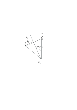
Figure 3: The geometric interpretation of the TB and TSB for binary linear codes.

III-B5 Reduction to Binary Linear Codes

Similarly, for binary linear codes, the transmitted codeword $\underline{s}$ can be assumed to be the all-zero codeword $\underline{s}^{(0)}$. The Euclidean distance between a codeword $\underline{\hat{s}}$ with Hamming weight $d$ and energy $\delta_{d_{2}}^{2}$ and $\underline{s}^{(0)}$ with energy $\delta_{d_{1}}^{2}$ is $\delta_{d}=2\sqrt{d}$. Note that $\delta_{d_{1}}=\delta_{d_{2}}=\sqrt{n}$, so $B_{\delta_{d_{1}},\delta_{d_{2}},\delta_{d}|\underline{s}^{(0)}}=A_{\delta_{d}|\underline{s}^{(0)}}$. See Fig. 3 for reference. Therefore, from (9), (33) and (36), the conditional union bound $f_{u}(z_{\xi_{1}}|\underline{s}^{(0)})$ can be written as

$$f_{u}(z_{\xi_{1}}|\underline{s}^{(0)}) = \sum_{\delta_{d_{1}},\delta_{d_{2}},\delta_{d}}B_{\delta_{d_{1}},\delta_{d_{2}},\delta_{d}|\underline{s}^{(0)}}p_{2}(z_{\xi_{1}},\delta_{d_{1}},\delta_{d_{2}},\delta_{d})$$ (40)

$$= \sum_{\delta_{d}}A_{\delta_{d}|\underline{s}^{(0)}}p_{2}(z_{\xi_{1}},\sqrt{n},\sqrt{n},\delta_{d})$$

$$= \sum_{1\leq d\leq n}A_{d}p_{2}(z_{\xi_{1}},d),$$

where

$$p_{2}(z_{\xi_{1}},d)=\int_{\beta_{d}(z_{\xi_{1}})}^{+\infty}\frac{1}{\sqrt{2\pi}\sigma}e^{-\frac{z_{\xi_{2}}^{2}}{2\sigma^{2}}}~{}{\rm d}z_{\xi_{2}},$$ (41)

and

$$\beta_{d}(z_{\xi_{1}})=\frac{\sqrt{d}(\sqrt{n}-z_{\xi_{1}})}{\sqrt{n-d}}.$$ (42)

$p_{2}(z_{\xi_{1}},d)$ is a strictly increasing and continuous function of $z_{\xi_{1}}$ such that $p_{2}(-\infty,d)=0$ and $p_{2}(\sqrt{n},d)=1/2$. Therefore,

$$f_{u}(z_{\xi_{1}}) = \sum_{\underline{s}}{\rm Pr}\{\underline{s}\}f_{u}(z_{\xi_{1}}|\underline{s})$$ (43)

$$= f_{u}(z_{\xi_{1}}|\underline{s}^{(0)})$$

$$= \sum_{1\leq d\leq n}A_{d}p_{2}(z_{\xi_{1}},d)$$

is also a strictly increasing and continuous function of $z_{\xi_{1}}$ such that $f_{u}(-\infty)=0$ and $f_{u}(\sqrt{n})\geq 3/2$. Hence there exists a unique solution $z_{\xi_{1}}^{*}\leq\sqrt{n}$ satisfying

$$\sum_{d=1}^{n}A_{d}p_{2}(z_{\xi_{1}},d)=1,$$ (44)

which is equivalent to that given in [1, (3.22)] by noticing that $p_{2}(z_{\xi_{1}},d)=Q\left(\frac{\sqrt{d}(\sqrt{n}-z_{\xi_{1}})}{\sigma\sqrt{n-d}}\right)$ and $d=\delta_{d}^{2}/4$.

The parameterized TB for binary linear codes can be written as

$${\rm Pr}\{E\} \leq \int_{-\infty}^{z_{\xi_{1}}^{*}}\!\!\!f_{u}(z_{\xi_{1}})g(z_{\xi_{1}})~{}{\rm d}z_{\xi_{1}}+\int_{z_{\xi_{1}}^{*}}^{+\infty}\!\!\!\!\!g(z_{\xi_{1}})~{}{\rm d}z_{\xi_{1}}$$ (45)

$$= \int_{-\infty}^{+\infty}\min\{f_{u}(z_{\xi_{1}}),1\}g(z_{\xi_{1}})~{}{\rm d}z_{\xi_{1}},$$

where $g(z_{\xi_{1}})$ and $f_{u}(z_{\xi_{1}})$ are given in (32) and (43), respectively. The optimal parameter $z_{\xi_{1}}^{*}$ is given by solving the equation (44). It can be shown that (45) is equivalent to that given in [1, (3.21)].

III-C The Parameterized Tangential-Sphere Bound

Assume that $n\geq 3$.

III-C1 Nested Regions

Again, the parameterized TSB chooses the nested regions to be a family of half-spaces $Z_{\xi_{1}}\leq z_{\xi_{1}}$, where $z_{\xi_{1}}\in\mathbb{R}$ is the parameter.

III-C2 Probability Density Function of the Parameter

The pdf of the parameter is

$$g(z_{\xi_{1}})=\frac{1}{\sqrt{2\pi}\sigma}e^{-\frac{z_{\xi_{1}}^{2}}{2\sigma^{2}}}.$$ (46)

III-C3 Conditional Upper Bound

Different from the parameterized TB, the parameterized TSB chooses $f_{u}(z_{\xi_{1}}|\underline{s})$ to be the conditional sphere bound when transmitting the codeword $\underline{s}$ over the channel. The conditional sphere bound given that $Z_{\xi_{1}}=z_{\xi_{1}}$ can be derived as follows.

Let $\mathcal{R}(r)$ be the $(n-1)$-dimensional sphere of radius $r>0$ which is centered at $(1-z_{\xi_{1}}/\delta_{d_{1}})\underline{s}$ and located inside the hyper-plane $Z_{\xi_{1}}=z_{\xi_{1}}$. See Fig. 2 for reference.

Given that the received vector $\underline{y}$ falls on the $(n-1)$-dimensional sphere $\partial\mathcal{R}(r)$ in the hyper-plane $Z_{\xi_{1}}=z_{\xi_{1}}$, the conditional pair-wise error probability is

$$p_{2}(z_{\xi_{1}},r,\delta_{d_{1}},\delta_{d_{2}},\delta_{d})=\left\{\begin{array}[]{rl}\frac{\Gamma(\frac{n-1}{2})}{\sqrt{\pi}~{}\Gamma(\frac{n-2}{2})}\int_{0}^{\arccos(\frac{\beta_{d}(z_{\xi_{1}})}{r})}\sin^{n-3}\phi~{}{\rm d}\phi,&r\geq\beta_{d}(z_{\xi_{1}}),\beta_{d}(z_{\xi_{1}})>0\\ 0,&r<\beta_{d}(z_{\xi_{1}}),\beta_{d}(z_{\xi_{1}})>0\\ 1-\frac{\Gamma(\frac{n-1}{2})}{\sqrt{\pi}~{}\Gamma(\frac{n-2}{2})}\int_{0}^{\arccos(\frac{|\beta_{d}(z_{\xi_{1}})|}{r})}\sin^{n-3}\phi~{}{\rm d}\phi,&r\geq|\beta_{d}(z_{\xi_{1}})|,\beta_{d}(z_{\xi_{1}})\leq 0\\ 1,&r<|\beta_{d}(z_{\xi_{1}})|,\beta_{d}(z_{\xi_{1}})\leq 0\end{array}\right.,$$ (47)

where

$$\beta_{d}(z_{\xi_{1}})=\frac{\delta_{d}-2z_{\xi_{1}}\cos{\theta}}{2\sin{\theta}},$$ (48)

and

$$\theta=\arccos\left(\frac{\delta_{d_{1}}^{2}+\delta_{d}^{2}-\delta_{d_{2}}^{2}}{2\delta_{d_{1}}\delta_{d}}\right).$$ (49)

From (24), we have the conditional sphere bound

$$f_{u}(z_{\xi_{1}}|\underline{s})=\int_{0}^{+\infty}\min\left\{f_{s}(z_{\xi_{1}},r|\underline{s}),1\right\}g_{s}(r)~{}{\rm d}r,$$ (50)

where

$$g_{s}(r)=\frac{2r^{n-2}e^{-\frac{r^{2}}{2\sigma^{2}}}}{2^{\frac{n-1}{2}}\sigma^{n-1}\Gamma(\frac{n-1}{2})},~{}~{}r\geq 0,$$ (51)

and

$$f_{s}(z_{\xi_{1}},r|\underline{s})=\sum_{\delta_{d_{1}},\delta_{d_{2}},\delta_{d}}B_{\delta_{d_{1}},\delta_{d_{2}},\delta_{d}|\underline{s}}p_{2}(z_{\xi_{1}},r,\delta_{d_{1}},\delta_{d_{2}},\delta_{d}).$$ (52)

III-C4 The Parameterized TSB

From (17), we have

$${\rm Pr}\{E|\underline{s}\} \leq \int_{-\infty}^{+\infty}\min\{f_{u}(z_{\xi_{1}}|\underline{s}),1\}g(z_{\xi_{1}})~{}{\rm d}z_{\xi_{1}}$$

$$\leq \int_{-\infty}^{+\infty}\min\left\{\int_{0}^{+\infty}\min\left\{f_{s}(z_{\xi_{1}},r|\underline{s}),1\right\}g_{s}(r)~{}{\rm d}r,1\right\}g(z_{\xi_{1}})~{}{\rm d}z_{\xi_{1}}.$$

From (3), we define

$$f_{s}(z_{\xi_{1}},r) \triangleq \sum_{\underline{s}}{\rm Pr}\{\underline{s}\}f_{s}(z_{\xi_{1}},r|\underline{s})$$ (54)

$$= \sum_{\underline{s}}{\rm Pr}\{\underline{s}\}\sum_{\delta_{d_{1}},\delta_{d_{2}},\delta_{d}}B_{\delta_{d_{1}},\delta_{d_{2}},\delta_{d}|\underline{s}}p_{2}(z_{\xi_{1}},r,\delta_{d_{1}},\delta_{d_{2}},\delta_{d})$$

$$= \sum_{\delta_{d_{1}},\delta_{d_{2}},\delta_{d}}B_{\delta_{d_{1}},\delta_{d_{2}},\delta_{d}}p_{2}(z_{\xi_{1}},r,\delta_{d_{1}},\delta_{d_{2}},\delta_{d}).$$

From (5), the parameterized TSB for general codes can be written as

$${\rm Pr\{E\}} = \sum_{\underline{s}}{\rm Pr}\{\underline{s}\}{\rm Pr}\{E|\underline{s}\}$$ (55)

$$\leq \sum_{\underline{s}}{\rm Pr}\{\underline{s}\}\int_{-\infty}^{+\infty}\min\left\{\int_{0}^{+\infty}\min\left\{f_{s}(z_{\xi_{1}},r|\underline{s}),1\right\}g_{s}(r)~{}{\rm d}r,1\right\}g(z_{\xi_{1}})~{}{\rm d}z_{\xi_{1}}$$

$$\leq \int_{-\infty}^{+\infty}\min\left\{\int_{0}^{+\infty}\min\left\{\sum_{\underline{s}}{\rm Pr}\left\{\underline{s}\right\}f_{s}(z_{\xi_{1}},r|\underline{s}),1\right\}g_{s}(r)~{}{\rm d}r,1\right\}g(z_{\xi_{1}})~{}{\rm d}z_{\xi_{1}}$$

$$= \int_{-\infty}^{+\infty}\min\left\{\int_{0}^{+\infty}\min\left\{f_{s}(z_{\xi_{1}},r),1\right\}g_{s}(r)~{}{\rm d}r,1\right\}g(z_{\xi_{1}})~{}{\rm d}z_{\xi_{1}},$$

which is determined by the triangle Euclidean distance spectrum $\{B_{\delta_{d_{1}},\delta_{d_{2}},\delta_{d}}\}$.

III-C5 Reduction to Binary Linear Codes

Similarly, for binary linear codes, the transmitted codeword $\underline{s}$ can be assumed to be the all-zero codeword $\underline{s}^{(0)}$. The Euclidean distance between a codeword $\underline{\hat{s}}$ with Hamming weight $d$ and energy $\delta_{d_{2}}^{2}$ and $\underline{s}^{(0)}$ with energy $\delta_{d_{1}}^{2}$ is $\delta_{d}=2\sqrt{d}$. Note that $\delta_{d_{1}}=\delta_{d_{2}}=\sqrt{n}$, so $B_{\delta_{d_{1}},\delta_{d_{2}},\delta_{d}|\underline{s}^{(0)}}=A_{\delta_{d}|\underline{s}^{(0)}}$. See Fig. 3 for reference. Therefore, from (50), the conditional sphere bound $f_{u}(z_{\xi_{1}}|\underline{s}^{(0)})$ can be written as

$$f_{u}(z_{\xi_{1}}|\underline{s}^{(0)})=\int_{0}^{+\infty}\min\left\{f_{s}(z_{\xi_{1}},r|\underline{s}^{(0)}),1\right\}g_{s}(r)~{}{\rm d}r.$$ (56)

From (9), (47) and (52), we have

$$f_{s}(z_{\xi_{1}},r|\underline{s}^{(0)}) = \sum_{\delta_{d_{1}},\delta_{d_{2}},\delta_{d}}B_{\delta_{d_{1}},\delta_{d_{2}},\delta_{d}|\underline{s}^{(0)}}p_{2}(z_{\xi_{1}},r,\delta_{d_{1}},\delta_{d_{2}},\delta_{d})$$ (57)

$$= \sum_{\delta_{d}}A_{\delta_{d}|\underline{s}^{(0)}}p_{2}(z_{\xi_{1}},r,\sqrt{n},\sqrt{n},\delta_{d})$$

$$= \sum_{1\leq d\leq n}A_{d}p_{2}(z_{\xi_{1}},r,d),$$

where

$$p_{2}(z_{\xi_{1}},r,d)=\left\{\begin{array}[]{rl}\frac{\Gamma(\frac{n-1}{2})}{\sqrt{\pi}~{}\Gamma(\frac{n-2}{2})}\int_{0}^{\arccos(\frac{\beta_{d}(z_{\xi_{1}})}{r})}\sin^{n-3}\phi~{}{\rm d}\phi,&r\geq\beta_{d}(z_{\xi_{1}}),z_{\xi_{1}}<\sqrt{n}\\ 0,&r<\beta_{d}(z_{\xi_{1}}),z_{\xi_{1}}<\sqrt{n}\\ 1-\frac{\Gamma(\frac{n-1}{2})}{\sqrt{\pi}~{}\Gamma(\frac{n-2}{2})}\int_{0}^{\arccos(\frac{|\beta_{d}(z_{\xi_{1}})|}{r})}\sin^{n-3}\phi~{}{\rm d}\phi,&r\geq|\beta_{d}(z_{\xi_{1}})|,z_{\xi_{1}}\geq\sqrt{n}\\ 1,&r<|\beta_{d}(z_{\xi_{1}})|,z_{\xi_{1}}\geq\sqrt{n}\end{array}\right.,$$ (58)

and

$$\beta_{d}(z_{\xi_{1}})=\frac{\sqrt{d}(\sqrt{n}-z_{\xi_{1}})}{\sqrt{n-d}}.$$ (59)

Then

$$f_{u}(z_{\xi_{1}}) = \sum_{\underline{s}}{\rm Pr}\{\underline{s}\}f_{u}(z_{\xi_{1}}|\underline{s})$$ (60)

$$= f_{u}(z_{\xi_{1}}|\underline{s}^{(0)}).$$

• Case 1: $Z_{\xi_{1}}=z_{\xi_{1}}\geq\sqrt{n}$. It can be shown that, given that received vector falls on $\partial\mathcal{R}(r)$, the pair-wise error probability is no less than 1/2. Hence the conditional union bound is no less than 3/2. From Theorem 1, we know that the optimal radius $r_{1}(z_{\xi_{1}})=0$, which results in the trivial upper bound $f_{u}(z_{\xi_{1}})\equiv 1$.

• Case 2: Given that $Z_{\xi_{1}}=z_{\xi_{1}}<\sqrt{n}$, the ML decoding error probability can be evaluated by considering an equivalent system in which each bipolar codeword is scaled by a factor $(\sqrt{n}-z_{\xi_{1}})/\sqrt{n}$ before transmitted over an AWGN channel with (projective) noise $(0,Z_{\xi_{2}},\cdots,Z_{\xi_{n}})$. The system is also equivalent to transmission of the original codewords over an AWGN but with scaled (projective) noise $\sqrt{n}/(\sqrt{n}-z_{\xi_{1}})(0,Z_{\xi_{2}},\cdots,Z_{\xi_{n}})$. The latter reformulation allows us to get the conditional sphere bound easily since the optimal radius is independent of the SNR. From (58), given that the received signal $\underline{y}$ falls on the $(n-1)$-dimensional sphere $\partial\mathcal{R}(r)$ in the hyper-plane $Z_{\xi_{1}}=0$, the conditional pair-wise error probability is

  $$\!\!\!\!\!p_{2}(0,r,d)\!\!=\!\!\frac{\Gamma(\frac{n-1}{2})}{\sqrt{\pi}~{}\Gamma(\frac{n-2}{2})}\int_{0}^{\arccos(\frac{\sqrt{nd/(n-d)}}{r})}\sin^{n-3}\phi~{}{\rm d}\phi$$

  if $r>\sqrt{nd/(n-d)}$ and $p_{2}(0,r,d)=0$ otherwise. Then we have the conditional sphere bound

  $$f_{u}(z_{\xi_{1}})=\int_{0}^{r_{1}}f_{s}(0,r|\underline{s}^{(0)})g_{s}(z_{\xi_{1}},r)~{}{\rm d}r+\int_{r_{1}}^{+\infty}g_{s}(z_{\xi_{1}},r)~{}{\rm d}r,$$ (61)

  where

  $$g_{s}(z_{\xi_{1}},r)=\frac{2r^{n-2}e^{-\frac{r^{2}}{2\tilde{\sigma}^{2}}}}{2^{\frac{n-1}{2}}\tilde{\sigma}^{n-1}\Gamma(\frac{n-1}{2})},~{}~{}r\geq 0,$$ (62)

  which depends on the SNR via $\tilde{\sigma}=\sqrt{n}\sigma/(\sqrt{n}-z_{\xi_{1}})$, and

  $$\!\!\!\!f_{s}(0,r|\underline{s}^{(0)})=\!\!\!\!\!\sum_{1\leq d\leq\frac{r^{2}n}{r^{2}+n}}A_{d}\frac{\Gamma(\frac{n-1}{2})}{\sqrt{\pi}~{}\Gamma(\frac{n-2}{2})}\int_{0}^{\arccos(\frac{\sqrt{nd/(n-d)}}{r})}\!\!\!\!\!\!\sin^{n-3}\phi~{}{\rm d}\phi,$$ (63)

  which is independent of $\tilde{\sigma}$, as justified previously. The optimal radius $r_{1}$ is the unique solution of

  $$\sum_{1\leq d\leq\frac{r^{2}n}{r^{2}+n}}A_{d}\frac{\Gamma(\frac{n-1}{2})}{\sqrt{\pi}~{}\Gamma(\frac{n-2}{2})}\int_{0}^{\arccos(\frac{\sqrt{nd/(n-d)}}{r})}\!\!\!\!\!\!\sin^{n-3}\phi~{}{\rm d}\phi=1.$$ (64)

  Since $r_{1}<+\infty$, $f_{u}(z_{\xi_{1}})<1$ for all $z_{\xi_{1}}<\sqrt{n}$.

• Summary: We have shown that the conditional sphere upper bound satisfying that $f_{u}(z_{\xi_{1}})<1$ if $z_{\xi_{1}}<\sqrt{n}$ and $f_{u}(z_{\xi_{1}})=1$ otherwise. Hence the optimal parameter $z_{\xi_{1}}^{*}=\sqrt{n}$.

The parameterized TSB for binary linear codes can be written as

$${\rm Pr}\{E\}\!\!\! \leq \!\!\!\int_{-\infty}^{\sqrt{n}}\!\!\!\!\!f_{u}(z_{\xi_{1}})g(z_{\xi_{1}})~{}{\rm d}z_{\xi_{1}}+\int_{\sqrt{n}}^{+\infty}\!\!\!\!\!g(z_{\xi_{1}})~{}{\rm d}z_{\xi_{1}},$$ (65)

where $g(z_{\xi_{1}})$ is given by (46), and $f_{u}(z_{\xi_{1}})$ is given by (61)-(64). To prove the equivalence of (65) to the formulae given in  [1, Sec.3.2.1], we first show that the optimal region is the same as that given in [1, Sec.3.2.1]. Noting that the optimal radius $r_{1}$ satisfies (64), which is equivalent to that given in [1, (3.12)]. Back to the hyper-plane $Z_{\xi_{1}}=z_{\xi_{1}}$, we can see that the optimal parameter is $r_{1}(\sqrt{n}-z_{\xi_{1}})/\sqrt{n}$. This means that the optimal region is a half-cone with the same angle as that given in [1, (3.12)]. Then, by changing variables, $r^{\prime}=r(\sqrt{n}-z_{\xi_{1}})/\sqrt{n}$, $z_{\xi_{2}}=r^{\prime}\cos\phi$, $v=r^{\prime 2}-z_{\xi_{2}}^{2}$ and $y=r^{\prime 2}$, it can be verified that (65) is equivalent to that given in [1, (3.10)], except that the second term ${\rm Pr}\{Z_{\xi_{1}}\geq\sqrt{n}\}$. This term did not appear in the original derivation of TSB in [10], but is required as pointed out in [22, Appendix A].

IV Numerical Results

As seen from Sec. III, computing the derived upper bounds requires the Euclidian distance spectrums, which are usually difficult to compute for general codes. In this section, we take general trellis code as an example to compare the derived bounds. In the case when the trellis complexity is reasonable, both the Euclidean distance enumerating function $A(X)$ defined in (2) and the triangle Euclidean distance enumerating function $B(X,Y,Z)$ defined in (4) are computable.

IV-A Trellis Code

A general code $\mathcal{C}(n,M)$ can be represented by a trellis. The trellis can have $N$ stages. The trellis section at stage $t$ $(0\leq t\leq N-1)$, denoted by $\mathcal{B}_{t}$, is a subset of $\mathcal{S}_{t}\times\mathbb{R}^{n_{t}}\times\mathcal{S}_{t+1}$, where $\mathcal{S}_{t}$ is the state space at stage $t$ and $n_{t}$ is the number of symbols associated with the $t$-th stage of the trellis. An element $b\in\mathcal{B}_{t}$ is called a branch and denoted by $b\stackrel{{\scriptstyle\Delta}}{{=}}(\sigma^{-}(b),\ell(b),\sigma^{+}(b))$, starting from a state $\sigma^{-}(b)\in\mathcal{S}_{t}$, taking a label $\ell(b)\in\mathbb{R}^{n_{t}}$, and ending into a state $\sigma^{+}(b)\in\mathcal{S}_{t+1}$. A path through a trellis is a sequence of branches ${\underline{b}}=(b_{0},b_{1},\cdots,b_{N-1})$ satisfying that $b_{t}\in\mathcal{B}_{t}$ and $\sigma^{-}(b_{t+1})=\sigma^{+}(b_{t})$. A codeword is then represented by a path in the sense that $\underline{s}=(\ell(b_{0}),\ell(b_{1}),\cdots,\ell(b_{N-1}))$. Naturally, $\sum_{0\leq t\leq N-1}n_{t}=n$, and the number of paths is $M$. Without loss of generality, we set $\mathcal{S}_{0}=\mathcal{S}_{N}=\{0\}$.

A trivial trellis representation of a general code $\mathcal{C}(n,M)$ has a single starting state, a single ending state and $M$ parallel branches, each of which is labeled by a codeword. For most trellis algorithms, the computational complexity is dominated by $\max|\mathcal{B}_{t}|$ and $\max|\mathcal{S}_{t}|$, as pointed out in [23] [24].

In this paper, we assume that both $\max|\mathcal{B}_{t}|$ and $\max|\mathcal{S}_{t}|$ are small-to-moderate. Typical examples include terminated trellis-coded modulation (TCM) [25] and terminated intersymbol interference (ISI) channels [26].

IV-B Product Error Trellis

For a general code represented by a (possibly time-invariant) trellis, we need the product error trellis to compute the Euclidean distance spectrums $\{A_{\delta_{d}}\}$ and $\{B_{\delta_{d_{1}},\delta_{d_{2}},\delta_{d}}\}$. The product error trellis has also $N$ stages. The trellis section at the $t$-th stage is $\mathcal{B}_{t}\times\mathcal{B}_{t}$. A branch $(b_{t},\hat{b}_{t})\in\mathcal{B}_{t}\times\mathcal{B}_{t}$ starts from state $(\sigma^{-}(b_{t}),\sigma^{-}(\hat{b}_{t}))\in\mathcal{S}_{t}\times\mathcal{S}_{t}$, takes a label $(\ell(b_{t}),\ell(\hat{b}_{t}))$, and ends into the state $(\sigma^{+}(b_{t}),\sigma^{+}(\hat{b}_{t}))$. A pair of codewords $(\underline{s},\underline{\hat{s}})$ correspond to a path $((b_{0},\hat{b}_{0}),(b_{1},\hat{b}_{1}),\dots,(b_{N-1},\hat{b}_{N-1}))$ through the product error trellis, where $(b_{0},b_{1},\dots,b_{N-1})$ is the path corresponding to the codeword $\underline{s}$ and $(\hat{b}_{0},\hat{b}_{1},\dots,\hat{b}_{N-1})$ is the path corresponding to the codeword $\underline{\hat{s}}$ . A single error event starting at the stage $i$ and ending at the stage $j$ is specified by a path $((b_{0},\hat{b}_{0}),(b_{1},\hat{b}_{1}),\dots,(b_{N-1},\hat{b}_{N-1}))$ satisfying that

• $b_{t}=\hat{b}_{t}$ for all $t\leq i-1$, $\sigma^{-}(b_{i})=\sigma^{-}(\hat{b}_{i})$.

• $\sigma^{+}(b_{t})\neq\sigma^{+}(\hat{b}_{t})$ for all $i\leq t\leq j-1$, $\sigma^{+}(b_{j})=\sigma^{+}(\hat{b}_{j})$.

• $b_{t}=\hat{b}_{t}$ for all $t>j$.

Since only single error events are required to calculate a tighter union bound [19][27], we have the following algorithms.

Algorithm 1

Compute the Euclidean distance enumerating functions.

1:  Initialize $\alpha_{t}(p)=0,\alpha^{\prime}_{t}(p)=0$, for $t\in[0,N],p\in\mathcal{S}_{t}\times\mathcal{S}_{t}$. $\alpha_{0}((0,0))=1$.

2:  for $t\in[0,N-1]$ do

3:     for $b,\hat{b}\in\mathcal{B}_{t}$ do

4:        $p=(\sigma^{-}(b),\sigma^{-}(\hat{b}))$

5:        $q=(\sigma^{+}(b),\sigma^{+}(\hat{b}))$

6:        $\gamma_{e}=X^{\|\ell(b)-\ell(\hat{b})\|^{2}}$

7:        if $b=\hat{b}$ then

8:           $\alpha^{\prime}_{t+1}(q)\leftarrow\alpha^{\prime}_{t+1}(q)+\alpha^{\prime}_{t}(p)\gamma_{e}$

9:           $\alpha_{t+1}(q)\leftarrow\alpha_{t+1}(q)+\alpha_{t}(p)\gamma_{e}$

10:        else

11:           if $\sigma^{+}(b)=\sigma^{+}(\hat{b})$ then

12:              $\alpha^{\prime}_{t+1}(q)\leftarrow\alpha^{\prime}_{t+1}(q)+\alpha_{t}(p)\gamma_{e}$

13:           else

14:              $\alpha_{t+1}(q)\leftarrow\alpha_{t+1}(q)+\alpha_{t}(p)\gamma_{e}$

15:           end if

16:        end if

17:     end for

18:  end for

19:  $A(X)=\alpha^{\prime}_{N}((0,0))/M$

20:  return  $A(X)$

Remark. To compute the triangle Euclidean distance enumerating function, we only need to replace $A(X)$ with $B(X,Y,Z)$ and define $\gamma_{e}=X^{\|\ell(b)\|^{2}}Y^{\|\ell(\hat{b})\|^{2}}Z^{\|\ell(b)-\ell(\hat{b})\|^{2}}$ in line 6.

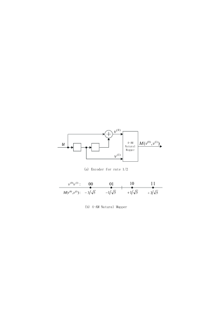
Figure 4: Realization of $4$-AM trellis code by means of a convolutional encoder.

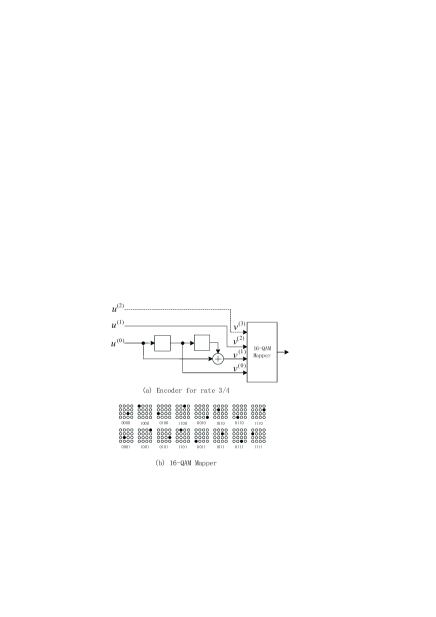
Figure 5: Realization of $16$-QAM trellis code by means of a minimal convolutional encoder [28].

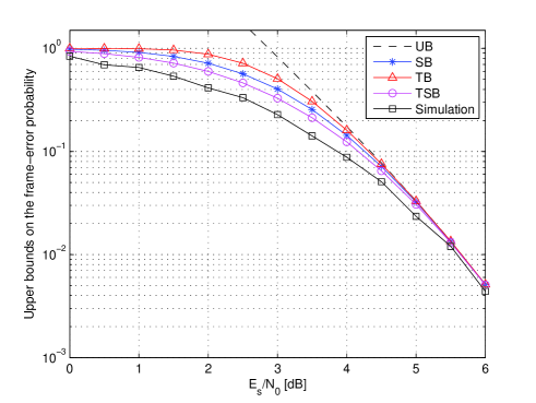
Figure 6: Upper bounds on the frame-error probability for the terminated trellis code $(32,2^{30})$ as shown in Fig. 4.

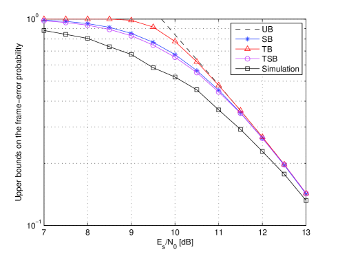
Figure 7: Upper bounds on the frame-error probability for the terminated trellis code $(24,2^{30})$ as shown in Fig. 5.

IV-C Numerical Results

Realizations of $4$-AM and $16$-QAM trellis codes by means of convolutional encoders are shown in Fig. 4 and Fig. 5, respectively, which result in transmitting signals with unequal energy over AWGN channels. From (6), (26), (39) and (55), the comparisons between the union bound, the parameterized SB, the parameterized TB, the parameterized TSB and the simulation result on the frame-error probability of the two terminated trellis codes are shown in Fig. 6 and Fig. 7, respectively.

V Conclusions

In this paper, we have presented a general framework to investigate Gallager’s first bounding technique with a single parameter to derive upper bounds on the ML decoding error probability of general codes. With the proposed parameterized GFBT, the SB, the TB and the TSB are generalized to general codes without the properties of geometrical uniformity and equal energy. It was shown that the SB can be calculated given that the Euclidean distance spectrum of the code is available and that both the TB and the TSB can be calculated given that the triangle Euclidean distance spectrum of the code is available. When applied to binary linear codes, the triangle distance spectrum is reduced to the conventional weight distribution. As a result, the three generalized bounds are reduced to the conventional ones. With the proposed parameterized GFBT, the equation for the optimal parameter can be obtained in an intuitive manner without resorting to the derivatives.

References

- [1] I. Sason and S. Shamai, “Performance analysis of linear codes under maximum-likelihood decoding: A tutorial,” in Foundations and Trends in Commun. and Inf. Theory. Delft, The Netherlands: NOW, July 2006, vol. 3, no. 1-2, pp. 1–225.
- [2] T. M. Duman and M. Salehi, “New performance bounds for turbo codes,” IEEE Trans. Inf. Theory, vol. 46, no. 6, pp. 717–723, June 1998.
- [3] T. M. Duman, “Turbo codes and turbo coded modulation systems: Analysis and performance bounds,” Ph.D. dissertation, Elect. Comput. Eng. Dept., Northeastern Univ., Boston, MA, May 1998.
- [4] N. Shulman and M. Feder, “Random coding techniques for nonrandom codes,” IEEE Trans. Inf. Theory, vol. 45, no. 6, pp. 2101–2104, September 1999.
- [5] M. Twitto, I. Sason, and S. Shamai, “Tightened upper bounds on the ML decoding error probability of binary linear block codes,” IEEE Trans. Inf. Theory, vol. 53, pp. 1495–1510, April 2007.
- [6] E. R. Berlekamp, “The technology of error correction codes,” Proceedings of the IEEE, vol. 68, pp. 564–593, May 1980.
- [7] T. Kasami, T. Fujiwara, T. Takata, K. Tomita, and S. Lin, “Evaluation of the block error probability of block modulation codes by the maximum-likelihood decoding for an AWGN channel,” in Proc. of the 15th Symp. Inf. Theory and Its Applications, Minakami, Japan, September 1992.
- [8] T. Kasami, T. Fujiwara, T. Takata, and S. Lin, “Evaluation of the block error probability of block modulation codes by the maximum-likelihood decoding for an AWGN channel,” in Proc. 1993 IEEE Int. Symp. Inf. Theory, January 1993, p. 68.
- [9] H. Herzberg and G. Poltyrev, “Techniques of bounding the probability of decoding error for block coded modulation structures,” IEEE Trans. Inf. Theory, vol. 40, pp. 903–911, May 1994.
- [10] G. Poltyrev, “Bounds on the decoding error probability of binary linear codes via their spectra,” IEEE Trans. Inf. Theory, vol. 40, pp. 1284–1292, July 1994.
- [11] D. Divsalar, “A simple tight bound on error probability of block codes with application to turbo codes,” in Proc. 1999 IEEE Commun. Theory Workshop, Aptos, CA, May 1999.
- [12] D. Divsalar and E. Biglieri, “Upper bounds to error probabilities of coded systems beyond the cutoff rate,” IEEE Trans. Commun., vol. 51, no. 12, pp. 2011–2018, December 2003.
- [13] S. Yousefi and A. K. Khandani, “A new upper bound on the ML decoding error probability of linear binary block codes in AWGN interference,” IEEE Trans. Inf. Theory, vol. 50, pp. 3026–3036, Novomber 2004.
- [14] ——, “Generalized tangential sphere bound on the ML decoding error probability of linear binary block codes in AWGN interference,” IEEE Trans. Inf. Theory, vol. 50, pp. 2810–2815, Novomber 2004.
- [15] A. Mehrabian and S. Yousefi, “Improved tangential sphere bound on the ML decoding error probability of linear binary block codes in AWGN and block fading channels,” IEE Proc. Commun., vol. 153, pp. 885–893, December 2006.
- [16] X. Ma, C. Li, and B. Bai, “Maximum likelihood decoding analysis of LT codes over AWGN channels,” in Proc. of the 6th Int. Symp. on Turbo Codes and Iterative Information Processing, Brest, France, September 2010.
- [17] X. Ma, J. Liu, and B. Bai, “New techniques for upper-bounding the MLD performance of binary linear codes,” in Proc. 2011 IEEE Int. Symp. Inf. Theory, Saint-Petersburg, Russian Federation, August 2011, pp. 2910–2914.
- [18] ——, “New techniques for upper-bounding the ML decoding performance of binary linear codes,” IEEE Trans. Commun., vol. 61, no. 3, pp. 842–851, Mar. 2013.
- [19] G. Caire and E. Viterbo, “Upper bound on the frame error probability of terminated trellis codes,” IEEE Commun. Lett., vol. 1, no. 1, pp. 2–4, Jan. 1998.
- [20] E. Agrell, “Voronoi regions for binary linear block codes,” IEEE Trans. Inf. Theory, vol. 42, pp. 310–316, January 1996.
- [21] ——, “On the Voronoi neighbor ratio for binary linear block codes,” IEEE Trans. Inf. Theory, vol. 44, pp. 3064–3072, Novomber 1998.
- [22] I. Sason and S. Shamai, “Improved upper bounds on the ML decoding error probability of parallel and serial concatenated turbo codes via their ensemble distance spectrum,” IEEE Trans. Inf. Theory, vol. 46, pp. 24–47, January 2000.
- [23] R. J. McEliece, “On the BCJR trellis for linear block codes,” IEEE Trans. Inf. Theory, vol. 42, pp. 1072–1092, July 1996.
- [24] X. Ma and A. Kavčić, “Path partition and forward-only trellis algorithms,” IEEE Trans. Inf. Theory, vol. 49, no. 1, pp. 38–52, Jan. 2003.
- [25] G. Ungerboeck, “Trellis-coded modulation with redundant signal sets-part I: Introdution and part II: State of the art,” IEEE Commun. Mag., vol. 25, pp. 5–21, Feb 1987.
- [26] G. D. Forney Jr., “Maximum-likelihood sequence estimation of digital sequences in the presence of intersymbol interference,” IEEE Trans. Inf. Theory, vol. 18, pp. 363–378, March 1972.
- [27] H. Moon and D. C. Cox, “Improved performance upper bounds for terminated convolutional codes,” IEEE Commun. Lett., vol. 11, no. 6, pp. 519–521, June 2007.
- [28] G. Ungerboeck, “Channel coding for multilevel/phase signals,” IEEE Trans. Inf. Theory, vol. IT-28, pp. 55–67, Jan. 1982.