Experimental realization of a quantum phase transition of polaritonic excitations
Abstract
We report an experimental realization of the Jaynes-Cummings-Hubbard (JCH) model using the internal and radial phonon states of two trapped ions. An adiabatic transfer corresponding to a quantum phase transition from a localized insulator ground state to a delocalized superfluid (SF) ground state is demonstrated. The SF phase of polaritonic excitations characteristic of the interconnected Jaynes-Cummings (JC) system is experimentally explored, where a polaritonic excitation refers to a combination of an atomic excitation and a phonon interchanged via a JC coupling.
pacs:
03.67.Ac, 37.10.TyThe Jaynes-Cummings (JC) model Jaynes and Cummings (1963); Meekhof et al. (1996) describing the interaction between a quantized optical mode and a two-level atom is one of the simplest and most important models of light-matter interactions. An interconnected array of multiple JC systems has recently been attracting interest, and the model describing it is referred to as the Jaynes-Cummings-Hubbard (JCH) model Greentree et al. (2006); Hartmann et al. (2006); Angelakis et al. (2007); Rossini and Fazio (2007); Irish et al. (2008); Makin et al. (2008); Ivanov et al. (2009); an experimental realization of this model has remained to be done. The JCH model was originally proposed for an array of coupled optical cavities, each containing a two-level atom, and is expected to exhibit properties peculiar to strongly correlated systems Hubbard (1963); van der Zant et al. (1992); Greiner et al. (2002).
In the JCH model for an array of coupled optical cavities, photons naturally hop between neighboring cavities, whereas the photon-photon interaction arises from a photon blockade Rebic et al. (2002), which impedes other photons from entering an occupied cavity.
The JCH model has certain similarities to the Bose-Hubbard (BH) model van der Zant et al. (1992); Greiner et al. (2002). It approaches the pure bosonic case in the large detuning and the large photon number limits Greentree et al. (2006). In contrast, in the limit of small detuning and small phonon numbers, the coefficient for the on-site repulsion becomes dependent on the photon number. In addition, the conserved particles (polaritons or dressed atoms) transform into various kinds of excitations (atomic excitations, photons or polaritons) depending on the Rabi frequency and detuning. As a result, a JCH system has a richer phase structure compared with a BH system. Both photons and polaritons can show superfluidity, while insulator phases can be formed with both atoms and polaritons Rossini and Fazio (2007); Irish et al. (2008).
Recent advances in the ability to manipulate quantum systems have made it possible to simulate a quantum system using another controllable system (analog quantum computation) Feynman (1982). Trapped ions offer high controllability and individual access, and hence are suited for such applications Johanning et al. (2009); Blatt and Roos (2012). Simulations of systems including spin systems and relativistic electrons have been reported Friedenauer et al. (2008); Gerritsma et al. (2010); Kim et al. (2010); Lanyon et al. (2011); Islam et al. (2011). Simulations of Hubbard models have also been proposed for trapped ions Porras and Cirac (2004); Ivanov et al. (2009), however an experimental demonstration has remained to be done.
The phonons in the radial (or transverse) direction of a linear ionic chain, which have been used to mediate spin-spin interactionsKim et al. (2010); Islam et al. (2011), can also be used to simulate systems of Bosonic particles under certain conditions Porras and Cirac (2004). In contrast to the axial motion of ions in a linear chain, which is described by collective modes that span over the whole ionic chain, radial phonons under a sufficiently tight radial confinement are essentially ’local phonons’ (phonons of local harmonic oscillations) undergoing hopping from site to site with a rate slower than the local harmonic-oscillation frequencies. We recently observed this hopping of radial phonons using two trapped ionsHaze et al. (2012). Ivanov et al.Ivanov et al. (2009) proposed to use a JC coupling arising from optical excitation of the radial red sideband transition of a linear ionic chain to induce an effective phonon-phonon coupling, thereby realizing the JCH model. In this letter, we report an experimental realization of the JCH model and observation of a quantum phase transition based on Ivanov et al.Ivanov et al. (2009) In this case the conserved particles are not merely phonons but composite particles each of which is a linear combination of a phonon and an atomic excitation.
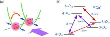
The conceptual schematic of the JCH system using trapped ions is shown in Fig. 1(a). It is assumed that two ions with internal states and a resonance frequency are held in a linear Paul trap. Each of the ions undergoes harmonic motion in a radial direction (referred to as the direction). Both ions are equally illuminated with a laser of frequency and detuning , which is nearly resonant with the radial red-sideband transitions. Then the system is approximately governed by the following Hamiltonian (a JCH Hamiltonian) Ivanov et al. (2009):
| (1) | |||||
Here is the detuning from the radial red-sideband transition, where is the oscillation frequency for the radial direction, in which is the oscillation frequency of a single ion in the radial direction and is the correction due to the Coulomb interaction ( is the inter-ion distance and is the mass of one ion). is the coupling coefficient for the red sideband transition (JC coupling) where is the Lamb-Dicke factor and is the on-resonance Rabi frequency. and are the creation and annihilation operators of phonons in the radial -direction of the -th ion, whose Hilbert space is spanned by Fock-state basis (). and are the raising and lowering operators for the internal states. is the hopping rate for the radial direction.
A JCH system is expected to show quantum phase transitions between superfluid and insulator phases of polaritons Angelakis et al. (2007). Here a ’superfluid’ is a system that has delocalized excitations and in which there is a correlation between mechanical variables at different sites. On the other hand, an ’insulator’ is a system that has localized excitations.
As an order parameter characterizing the quantum phase transition, the variance of the total excitation number per site, , where , can be used Angelakis et al. (2007). The expectation value of the annihilation operator which is usually used in the mean-field limit cannot be used as the order parameter, since it is always zero for a closed system with no particle exchange with the outsideAngelakis et al. (2007); Irish et al. (2008). In addition, the atomic excitation number variance , where , is also used for judging the existence of polaritons.
The experimental setup used is similar to that described in Haze et al. (2012) and a brief description is given here. Two 40Ca+ ions are trapped in vacuum ( Pa) using a linear Paul trap. A RF voltage of 25 MHz is applied to generate the radial confinements and DC electrodes provide an axial confinement. The secular frequencies for the three trap axes are MHz. The inter-ion distance in the axial direction is 18–20 m and correspondingly, the hopping rate is 5–7 kHz.
The energy levels relevant to motional cooling and induction of the JC coupling are shown in Fig. 1(b). The motion in the radial directions is cooled by Doppler cooling using – (397 nm) and –(866 nm) and sideband cooling using – (729 nm) and –(854 nm). There is two collective modes in the direction of two ions, namely the center-of-mass (COM; in-phase) mode and the rocking (out-of-phase) mode, just as in the case of the axial motion James (1998). The average quantum numbers after the sideband cooling are . The axial motion is cooled only by Doppler cooling. The ions are intermittently optically pumped to by using a 397-nm beam with the polarization during and after the sideband cooling. The excitation beam at 729 nm for the – transition, which is used to induce the JC coupling and other operations, is oriented at 45∘,45∘, and 90∘ relative to the , , and directions, respectively. This direction is chosen to couple the beam only to the radial directions and to ignore the axial directions, whose secular frequency is relatively small and hence less advantageous in sideband cooling because of the large average quantum number after Doppler cooling. Equal illumination of the two ions with this beam is carefully optimized by adjusting the beam position so that the intensity difference between the two ions becomes less than 5%.
The internal state of the ions is determined by illuminating them with lasers at 397 nm (– transition) and 866 nm (– transition) and by detecting fluorescence photons with a photomultiplier or an intensified charge-coupled-device (ICCD) camera, with detection times of 8 ms and 80 ms, respectively. Individual detection of fluorescence from each ion is possible with the ICCD camera. Due to unequal illumination intensity of the two ions with the 397 nm laser, individual detection is possible also when using the photomultiplier.
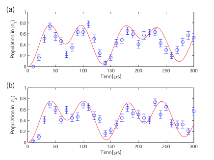
First, the dynamics of the JCH system with two ions is observed. The total dynamics of the two-ion JCH system arises from the JC coupling in individual atoms excited by the excitation laser and inter-site hoppingHaze et al. (2012). When the hopping rate is much smaller than the JC coupling coefficient , a simple sinusoidal oscillation similar to Rabi dynamics caused by the sideband excitation of the local radial oscillation modes is expected, while for non-negligible values of , an interference between Rabi and hopping dynamics is expected. Figure 2 shows the result of the observation of the JCH dynamics for two ions (the circles), where the population of the internal state of each ion is plotted. The system is initially prepared in the state with sideband cooling and optical pumping. The excitation laser is tuned to the resonance of the blue-sideband transition of the radial mode. This gives rise to an anti-Jaynes-Cummings coupling Meekhof et al. (1996), which is formally equivalent to a JC coupling when the internal states are interchanged. The red curves show numerically simulated dynamics for the hopping rate of 5.4 kHz, the JC coupling coefficient of 12.0 kHz, and the coherence relaxation due to laser frequency fluctuations of 200 Hz. Although the dynamics is periodical, it is greatly modified from a simple sinusoidal oscillation due to the effect of the inter-site hopping term. The two ions show almost the same dynamics as expected from equal illumination.
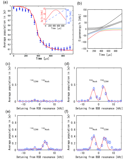
As a demonstration of a quantum phase transition, an adiabatic transfer from an insulator ground state to a SF ground state is observed in the average excited-state population of two ions [Fig. 3 (a)].
The transfer process starts from a point where is large, where the ground state is approximately (the atomic insulator phase). Then increases, exceeds zero and becomes a large positive value, where the ground state is approximately . Here, is the rocking-mode creation operator. This phase is the phonon SF phase. In the intermediate region around , the system is in the polaritonic SF state. This polaritonic SF state is approximated as Irish et al. (2008).
In the experiment, is prepared with cooling, optical pumping and applying a carrier pulse. Then the adiabatic transfer is realized by shining the excitation laser and sweeping its detuning over the red-sideband resonance from negative to positive values. The amplitude of the beam is also modulated in a Gaussian shape to ensure that is large at the beginning and end of the pulse so that the overlap of the initial (final) state and () is optimized. The explicit values of the parameters are as follows. is linearly swept from -41 kHz to 59 kHz in 960 s, and the JC coupling coefficient is varied from 0.2914 kHz to 14 kHz and back to 0.2914 kHz in a Gaussian shape over the same period [see the inset of Fig. 3 (a)]. The red curve in Fig. 3 (a) is a numerically simulated result.
The initial population in Fig. 3 (a) is 5 % smaller than what is expected for . This is the result of infidelity in the carrier pulse used to prepare , which is presumably due to jitter in the excitation beam. The final population is floating from zero by 10 %. In addition to the imperfect initialization mentioned above, this is due also to infidelity in the adiabatic transfer process itself, which we speculate is due mainly to the effect of laser frequency fluctuations. We previously analyzed the effects of laser frequency fluctuations and adiabaticity in the rapid adiabatic passage on the sideband transitions (Fig. 4 of Watanabe et al. (2011); although this analysis was done for a single ion, the overall qualitative and quantitative behavior should be similar). We have confirmed in a numerical simulation that the population go to near zero with less than 1 % error under the assumption of no laser frequency fluctuation. Hence we speculate that the effect of diabatic transitions is limited to below 1 %.
We also analyzed the adiabaticity during the transfer process using the theory of adiabatic variations of HamiltoniansMessiah1961 . Fig. 3 (b) shows the time-dependent eigenenergies obtained by diagonalyzing the instantaneous Hamiltonians based on the pulse parameters used in the experiment. From these eigenenergies and eigenvectors, the probability of diabatic transitions is estimated in a similar way as in Watanabe et al. (2011). The largest leakage from the ground state is the one towards the third lowest level, and its probability is at most 2 %. This is consistent with the numerical result given above.
The effect of the adiabatic transfer process on the phonon states is also examined. Figure 3 (c)-(f) shows the result of phonon-number measurements. Figure 3 (c) and (d) show the results of spectroscopy over the radial red- and blue-sideband transitions, respectively, at the beginning of the adiabatic transfer process, and Figure 3 (e) and (f) show the corresponding results at the end of the process. From these results, the average phonon numbers for the COM and rocking modes at the beginning and end are estimated to be and , respectively. At the beginning, both of the phonon modes are almost in the ground states, while at the end, a number of rocking-mode phonon quanta close to two is realized and the COM mode is almost intact. The above results support the occurrence of a quantum phase transition from the atomic insulator ground state to the phonon SF ground state .
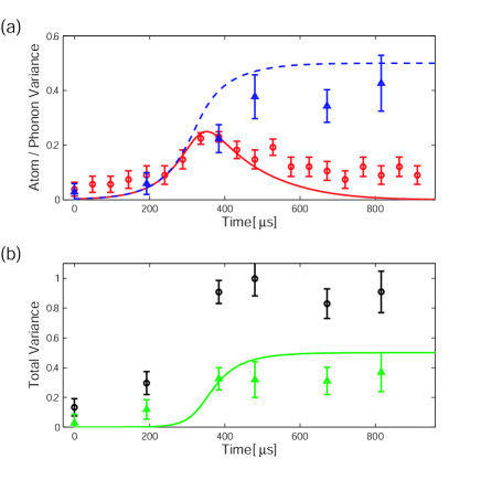
The transfer process is further analyzed by estimating the excitation number variances (atomic, phonon and total) introduced above. The red circles in Fig. 4 (a) show the atomic excitation number variance estimated from atomic populations measured with the photomultiplier tube. The peak at the center indicates the presence of polaritons. The numerically simulated results are also shown as the red solid curve. The cause for the discrepancy between the experimental and calculated values is expected to be similar to that discussed in relation to Fig. 3 (a). The blue triangles in Fig. 4 (a) show the values of the phonon number variance with , which are obtained by measuring the average phonon numbers in the same way as in Fig. 3 (c)-(f), and estimating the variance according to equation (3) and (4) of the Supplemental material. This supports the argument that the phonon SF ground state is realized at the end of the adiabatic transfer.
Estimation of the total excitation number variance requires simultaneous measurements of internal and phonon states, which are relatively difficult to perform since phonon states should be once mapped to internal states to be read. We avoid such measurements here and instead estimate from the known quantities and . It should be noted that in this case can only be estimated as intervals with upper and lower bounds. The details of the derivation of inequalities for estimating the upper and lower bounds of are given in the Supplemental material.
Figure 4 (b) is the total excitation number variance . The values (upper and lower bounds) are obtained using equation (5) and (6) of the Supplemental material along with the results in Fig. 4 (a). The expected qualitative behavior, including the onset of a phase transition (near 400 s), an example of which is seen in Fig. 2 of Angelakis et al. (2007), is reproduced in these results.
In summary, we have observed dynamics and adiabatic transfer between ground states of a JCH system with two ions. Scaling up the JCH system described in this article to include a larger numbers of sites necessitates certain points to be overcome. When the number of ions in the linear chain is increased, the spacing at the center decreases in proportion to James (1998) and hence increases in proportion to . On the other hand, it is desired to keep at moderate values so that the rich phase diagram of the JCH system should be explored as widely as possible. This demand may be fulfilled by tightening the radial confinement (note that ) or by using an array of independent traps, for which inter-ion distances and magnitudes of confinement can be chosen independently.
References
- Jaynes and Cummings (1963) E. T. Jaynes and F. W. Cummings, Proc. IEEE 51, 89 (1963).
- Meekhof et al. (1996) D. M. Meekhof, C. Monroe, B. E. King, W. M. Itano, and D. J. Wineland, Phys. Rev. Lett. 76, 1796 (1996).
- Greentree et al. (2006) A. D. Greentree, C. Tahan, J. H. Cole, and L. C. L. Hollenberg, Nature Phys. 2, 856 (2006).
- Hartmann et al. (2006) M. J. Hartmann, F. Brandao, and M. B. Plenio, Nature Phys. 2, 849 (2006).
- Angelakis et al. (2007) D. G. Angelakis, M. F. Santos, and S. Bose, Phys. Rev. A 76, 031805 (2007).
- Rossini and Fazio (2007) D. Rossini and R. Fazio, Phys. Rev. Lett. 99, 186401 (2007).
- Irish et al. (2008) E. K. Irish, C. D. Ogden, and M. S. Kim, Phys. Rev. A 77, 033801 (2008).
- Makin et al. (2008) M. I. Makin, J. H. Cole, C. Tahan, L. C. L. Hollenberg, and A. D. Greentree, Phys. Rev. A 77, 053819 (2008).
- Ivanov et al. (2009) P. A. Ivanov, S. S. Ivanov, N. V. Vitanov, A. Mering, M. Fleischhauer, and K. Singer, Phys. Rev. A 80, 060301 (2009).
- Hubbard (1963) J. Hubbard, Proc. R. Soc. A 276, 238 (1963).
- van der Zant et al. (1992) H. S. J. van der Zant, F. C. Fritschy, W. J. Elion, L. J. Geerligs, and J. E. Mooij, Phys. Rev. Lett. 69, 2971 (1992).
- Greiner et al. (2002) M. Greiner, O. Mandel, T. Esslinger, T. W. Hansch, and I. Bloch, Nature 415, 39 (2002).
- Rebic et al. (2002) S. Rebic, A. S. Parkins, and S. M. Tan, Phys. Rev. A 65, 063804 (2002).
- Feynman (1982) R. P. Feynman, Int. J. Theor. Phys. 21, 467 (1982).
- Johanning et al. (2009) M. Johanning, A. F. Varon, and C. Wunderlich, J. Phys. B 42, 154009 (2009).
- Blatt and Roos (2012) R. Blatt and C. F. Roos, Nature Phys. 8, 277 (2012).
- Friedenauer et al. (2008) A. Friedenauer, H. Schmitz, J. T. Glueckert, D. Porras, and T. Schaetz, Nature Phys. 4, 757 (2008).
- Gerritsma et al. (2010) R. Gerritsma, G. Kirchmair, F. Zahringer, E. Solano, R. Blatt, and C. F. Roos, Nature 463, 68 (2010).
- Kim et al. (2010) K. Kim, M. S. Chang, S. Korenblit, R. Islam, E. E. Edwards, J. K. Freericks, G. D. Lin, L. M. Duan, and C. Monroe, Nature 465, 590 (2010).
- Lanyon et al. (2011) B. P. Lanyon, C. Hempel, D. Nigg, M. Muller, R. Gerritsma, F. Zahringer, P. Schindler, J. T. Barreiro, M. Rambach, G. Kirchmair, et al., Science 333, 57 (2011).
- Islam et al. (2011) R. Islam, E. E. Edwards, K. Kim, S. Korenblit, C. Noh, H. Carmichael, G. D. Lin, L. M. Duan, C. C. J. Wang, J. K. Freericks, et al., Nat. Commun. 2, 377 (2011).
- Porras and Cirac (2004) D. Porras and J. I. Cirac, Phys. Rev. Lett. 93, 263602 (2004).
- Haze et al. (2012) S. Haze, Y. Tateishi, A. Noguchi, K. Toyoda, and S. Urabe, Phys. Rev. A 85, 031401 (2012).
- James (1998) D. F. V. James, Appl. Phys. B 66, 181 (1998).
- Watanabe et al. (2011) T. Watanabe, S. Nomura, K. Toyoda, and S. Urabe, Phys. Rev. A 84, 033412 (2011).
- (26) A. Messiah, Quantum Mechanics(North-Holland, Amsterdam, 1961), Vol. 2.
Acknowledgments
This work was supported by the Ministry of Education, Culture, Sports, Science and Technology (MEXT) of Japan Kakenhi ”Quantum Cybernetics” project, and by the Japan Society for the Promotion of Science (JSPS) through its Funding Program for World-Leading Innovative R&D on Science and Technology (FIRST Program).