Ising models on the Regularized Apollonian Network
Abstract
We investigate the critical properties of Ising models on a Regularized Apollonian Network (RAN), here defined as a kind of Apollonian Network (AN) in which the connectivity asymmetry associated to its corners is removed. Different choices for the coupling constants between nearest neighbors are considered, and two different order parameters are used to detect the critical behaviour. While ordinary ferromagnetic and anti-ferromagnetic models on RAN do not undergo a phase transition, some anti-ferrimagnetic models show an interesting infinite order transition. All results are obtained by an exact analytical approach based on iterative partial tracing of the Boltzmann factor as intermediate steps for the calculation of the partition function and the order parameters.
pacs:
89.75.Hc, 64.60.A-, 89.20.Hh, 89.75.DaMany real world networks exhibit complex topological properties as the small word effect, related to a very short minimal path between nodes, and the scale-free property, related to the power-law nature of the connectivity distribution. These properties have important implications in the real phenomena as virus spreading in computers, sharing of technological information and diffusion of epidemic diseases, to name just a few.
In this context, the Apollonian network AHAS2005 is a particularly useful theoretical tool, since it is scale-free, displays small-world effect, can be embedded in a Euclidean lattice and shows space-filling as well as matching graph properties. Therefore, in spite of its deterministic nature, it shares the most relevant characteristics of real world networks.
Phase transitions has been detected for a number of different physical models on Apollonian Networks. For example, the ideal gas undergoes to Bose-Einstein condensation CAS2008 ; 0MLAA2009 ; 0MLAA2010 ; 0MCL2010 ; OSMLS2013 and epidemics exhibits a transition between an absorbing state and an active state SCSMFA2013 ; SCCMSFA2013 . In particular, in OSMLS2013 it has been adopted an analytical strategy which has some similarities with that in this paper.
In this work we focus on the infinite order transition exhibited by some Ising models on the Apollonian network. Previous studies of similar Ising models AH2005 ; AAH2009 and Potts model AAH2010 have not detected critical properties, due to the fact that infinite order transitions are elusive. On the contrary, a second order phase transition, as a function of the noise parameter, has been detected for a majority vote model LMA2012 .
Ising models on different hierarchical fractal have been studied GF1982 and in the case of diamond fractal they have been exactly solved by exact renormalization DSI1983 ; BZ1989 . These models, differently to present model, show a second order phase transition. Indeed, the standard Ising behavior is second order transition in plane models S2010 ; S2011 , nevertheless, it may be very intricate, with many phases PS1997 , when the interactions are made more complicated.
We start by regularizing the standard Apollonian Network in order to remove the connectivity asymmetry associated to its corners which consistently simplify the analytical computation of the thermodynamics of the Ising models.
The Regularized Apollonian Network () is defined starting form a generation network with 4 nodes all connected, forming a tetrahedral structure with 6 bonds. Each of the four triples of nodes individuates a different triangle. At generation a new node is added inside each of the four triangles and it is connected with the surrounding three nodes, creating 12 new triangles. Then the procedure is iterated at any successive generation inserting new nodes in the last created triangles, and connecting each of them with the three surrounding nodes.
In the connectivity of any of the already existing nodes (so-called old nodes) is doubled when generation is updated, while the connectivity of the newly created nodes (the new nodes) always equals 3, leading to the following relevant property: the connectivity at generation of a node only depends on its age. More explicitly, its connectivity is where is the generation in which it was created. Besides, has the following properties: (i) the total number of nodes is ; (ii) the number of new nodes created at generation is (equality for large ); (iii) the average connectivity is (for large ); (iv) the total number of bonds is ; ) the number of new bonds created at generation is .
The number of nodes having coordination is which equals if with ; equals 4 if ; and equals otherwise. Accordingly, the cumulative distribution exhibits, for large values of , a power-law behavior i.e., , with .
Analogously to AN, RAN is scale-free and displays the small word effect. Furthermore, since RAN network can be decomposed in four AN networks cutting a finite number of couplings, the thermodynamics on the two models is the same.
Ising models are defined according to the following Hamiltonian:
| (1) |
where the first sum goes on all connected pairs of nodes of of generation , the second sum goes on all nodes, and the third sum only goes on the triangles of the last generation (one of the nodes or must be lastly generated). The constants and may depend on the connectivities (on the age) of the involved nodes. The couplings can be both positive (ferromagnetic) or negative (anti-ferromagnetic). The constant is introduced only for technical reasons, the relevant physics corresponding to .
The partition function is
| (2) |
where the sum goes on all configurations and is the inverse temperature, i.e., (we consider an unitary Boltzmann’s constant ). Then, the thermodynamical variables can be obtained from
| (3) |
Our strategy consists in performing a partial sum in (2) with respect to the spin variables over nodes created at the last generation . This sum creates new effective interaction between all remaining spins and new magnetizations, and a new value for the parameter . In other words, we exactly map the generation model in the same model with new parameters. This technique works for any possible choice of the parameters , and , but we will consider here only some simple cases.
We stress that our approach is different when compared to the transfer matrix technique AH2005 ; AAH2009 and it gives exact expressions for the thermodynamical variables in the limit. While it confirms the absence of transition in the ordinary ferromagnetic and anti-ferromagnetic models, it detects an infinite order phase transition in a simple anti-ferrimagnetic model occurring at a finite temperature, in contrast with what was found in AH2005 ; AAH2009 , where no critical behavior at a finite temperature was identified for this kind of models.
In order to illustrate our strategy we start with the simplest case in which all interactions are equal (), and all . Without loss of generality, one can chose (ferromagnetism) or (anti-ferromagnetism).
Since a new node is only linked to three older surrounding nodes (it is created inside a triangle), the summation on the spin over a new node creates an extra-interaction among the three surrounding spins on the older nodes. Therefore, the partial sum on spins over new nodes in (2) yields, after some lengthy but straightforward calculations, the following equality
| (4) |
where
| (5) |
Also,
| (6) |
In (4), is the partition function of the same model at generation () with a different value ( has the same sign of ). Note that in RAN (contrary to AN) equality (4) is exact.
Performing the thermodynamical limit , one obtains from (4)
| (7) |
where we have used and . We have thus re-expressed the thermodynamical function in terms of , proving the absence of transition. In fact, since only depends on the product , and since the above equation can be iterated, a single non-analytical point would imply an infinite number of non-analytical points.
Iteration of (7) gives
| (8) |
where
| (9) |
with . If (ferromagnetism), the positive increase monotonically and diverge for large . On the contrary, if (anti-ferromagnetism) the negative converge to 0 for large . In both cases it is easy to verify that the sum (8) converges.


Since we have proven that the both constant coupling cases (the ferromagnet and the anti-ferromagnet one) do not undergo a phase transition, we now extend our scope to consider a different model.
Let us now come back to the Hamiltonian (1) and let us assume that the action of the external magnetic field is proportional to the connectivity of the node, i.e., where is the connectivity of node . Accordingly, we can define the following spontaneous magnetization:
| (10) |
where we have used . The notation indicates average with respect to the Gibbs measure, in such a way that satisfies . The rational for this choice is that it turns out to be the simplest tool in order to show the existence of an infinite order phase transition in an anti-ferrimagnetic model.
For the same practical reasons, we compute the defined as
| (11) |
where the sum only goes on the triangles of last generation . Note that the factor in the last term comes from the fact that in the limit one has , accordingly .
Since we have proven that a constant value for the couplings leads to absence of transition , we will assume now, on the contrary, that they depend on the connectivity of the nodes and (in turn, the connectivity of a node depends only on its age). The simplest age dependence for an anti-ferrimagnetic model is with if the connectivity of at least one of the two nodes or is 3 and otherwise. This is the same of assuming that for bonds involving nodes of last generation and otherwise.


Then, following the same procedure, we take a partial sum with respect to the spins over last created nodes and we obtain the exact equality
| (12) |
We stress that, while the initial anti-ferromagnetic model (described by ) had two possible values for the couplings ( and ), the effective model after partial sum (described by ) has the single value for all of them. The new parameters , , and can be again explicitly computed in terms of . Since we are only interested in thermodynamical potentials, like the spontaneous magnetization and coordination in the absence of external magnetic fields, what we really use are only the values of , , for and their derivatives with respect to and , in the limit and .
Assuming and one has that and are also equal to zero, and we obtain again (8) with given by (6). The difference is that ,
| (13) |
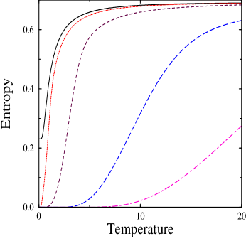
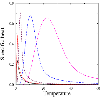
while the remaining for are again obtained by (9). The resulting entropy and specific heat, as a function of the temperature (in units of the Boltzmann’ constant ) are depicted in Fig. 1 and Fig. 2 for various values of . Note that the case is the regular anti-ferromagnet with non vanishing zero temperature entropy. Interestingly, whenever , as a consequence of the larger value of the coupling constants involving new nodes, frustration is removed and the zero temperature entropy drops to 0.
Let us call the (non vanishing) value of for which vanishes, which only depends on , then, there are three cases: (i) : in this case and one immediately obtains ; (ii) : in this case , i.e., the initial anti-ferrimagnetic model is mapped into a ferromagnetic model. The increases monotonically and diverges for large , (iii) : in this case , i.e., the initial anti-ferrimagnetic model is mapped into an anti-ferromagnetic model. The converge monotonically to 0 for large .
Is a critical point? The answer to this question is not easy since all thermodynamical functions seem to behave regularly at (see Figs. 1 and 2). To address this question we have to compute the spontaneous magnetization and the coordination .
Given in (12), it turns out that and , as well as and , calculated at vanish. Then, given (10) and (11), we obtain from (12): and where and are the magnetization and coordination of the model with couplings . Also,
| (14) |
where all derivative are calculated at .
This relation can be iterated and one obtains
| (15) |
where is the vector whose two elements are and ; are the matrices with elements and corresponds to spontaneous magnetization and coordination of the model with couplings .
If , the sequence of converges to 0, and is a vanishing matrix; therefore, independently on . If , on the contrary, one find that , with both component of equal to 1 (ferromagnet with infinitely large couplings). Furthermore, in this case, does not vanish, and therefore . We have thus proven the existence of a transition at .
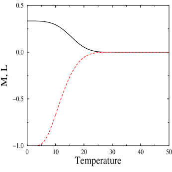
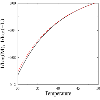
The magnetization and the for the model are depicted in the first panel of Fig 3. Apparently, the transition occurs at a temperature around 26, which is far from the transition temperature obtained by the non vanishing solution of with and . This is due to the fact that both and vanishes extremely slowly. In order to make this evident, we have depicted and in the second panel of Fig. 3, which clearly show agreement with the expected critical temperature . The behaviour of both magnetization and , close to the critical point, is compatible with the function , which implies an infinite order transition since and and all their derivatives are continuous at .
Note that a negative coordination implies that spins are preferentially organized, in order that in any triangle one of them points in the opposite direction of the other two. This organization becomes exact at where the coordination is -1. Observe also that, contrary to the anti-ferromagnetic model on regular lattices, the magnetization is positive below the critical temperature with a value compatible with 1/3 at .
Qualitatively identical results come out whenever , leading to: (i) individuates the transition temperature; (ii) the transition is of infinite order. In the limit one easily verify that , which confirms the absence of transition in the ordinary anti-ferromagnetic model.
Our minimal choice, for newly created bonds and otherwise, is the simplest but it is not the only one which leads to paramagnetic/ferromagnetic infinite order phase transition. Indeed, there are many possible hierarchical choices for the which lead to the same qualitative behavior.
The authors would like to thank the financial support from the Brazilian Research Agencies CAPES (Rede NanoBioTec and PNPD), CNPq [INCT-Nano(Bio) Simes, Casadinho] and FAPERN/CNPq (PRONEX). M.S. was partially supported by PRIN 2009 protocollo n. 2009TA2595.02.
References
- (1) J. S. Andrade, H. J. Herrmann, R. F. S. Andrade and L. R. da Silva, Phys. Rev. Lett. 94, 018702 (2005).
- (2) A. L. Cardoso, R. F. S. Andrade and A. M. C. Souza,, Phys. Rev. B 78, 214202 (2008).
- (3) I. N. de Oliveira, F. A. B. F. de Moura, M. L. Lyra, J. S. Andrade Jr. and E. L. Albuquerque, Phys. Rev. E 79, 016104 (2009).
- (4) I. N. de Oliveira, F. A. B. F. de Moura, M. L. Lyra, J. S. Andrade Jr. and E. L. Albuquerque, Phys. Rev. E 81, 030104R (2010).
- (5) I. N. de Oliveira, F. A. B. F. de Moura, R. A. Caetano and M. L. Lyra Phys. Rev. B 82, 172201 (2010).
- (6) I. N. de Oliveira, T. B. dos Santos, F. A. B. F. de Moura, M. L. Lyra and M. Serva, Phys. Rev. E, (in press, 2013).
- (7) L. F. da Silva, R. N. Costa Filho, D. J. B. Soares, A. Macedo-Filho, U. L. Fulco and E. L. Albuquerque, Phys. A 392, 1532-1537 (2013).
- (8) L. F. da Silva, R. N. Costa Filho, A. R. Cunha, A. Macedo-Filho, M. Serva, U. L. Fulco and E. L. Albuquerque, J. Stat. Mech.: Theory Exp., P05003 (2013).
- (9) R. F. S. Andrade and H. J. Herrmann, Phys. Rev. E 71, 056131 (2005).
- (10) R. F. S. Andrade, J.S. Andrade and H. J. Herrmann, Phys. Rev. E 79, 036105 (2009).
- (11) A. M. Araújo, R. F. S. Andrade and H.J. Herrmann, Phys. Rev. E 82, 046109 (2010).
- (12) F. W. S. Lima, A. A. Moreira and A. D. Araújo, Phys. Rev. E 86, 056109 (2012)
- (13) R. B. Griffiths and M. Kaufman Phys. Rev. B 26, 5022-5032 (1982).
- (14) B. Derrida, L. De Seze and C. Itzykson, Journal of Statistical Physics, 33, 559-569 (1983).
- (15) P. M. Bleher and E. Žalys Commun. Math. Phys. 120 409-436 (1989)
- (16) M. Serva, Phys. A 389, 2700-2707 (2010).
- (17) M. Serva, Phys. A 390, 2443-2451 (2010).
- (18) M. Pasquini and M. Serva, Phys. Rev. E 56, 2751-2756 (1997).