On integrability of zero-range chipping models with factorized steady state

Abstract

Conditions of integrability of general zero range chipping models with factorized steady state, which were proposed in [Evans, Majumdar, Zia 2004 J. Phys. A 37 L275], are examined. We find a three-parametric family of hopping probabilities for the models solvable by the Bethe ansatz, which includes most of known integrable stochastic particle models as limiting cases. The solution is based on the quantum binomial formula for two elements of an associative algebra obeying generic homogeneous quadratic relations, which is proved as a byproduct. We use the Bethe ansatz to solve an eigenproblem for the transition matrix of the Markov process. On its basis we conjecture an integral formula for the Green function of evolution operator for the model on an infinite lattice and derive the Bethe equations for the spectrum of the model on a ring.

Keywords: asymmetric simple exclusion process, zero-range process, Bethe ansatz, quantum binomial

1 Introduction

Integrability is a key feature of stochastic particle systems, which allows one to obtain plenty exact results. Often in a proper (scaling) limit these results become meaningful in a context of a whole universality class. The most prominent example is the asymmetric simple exclusion process (ASEP) [1]. Its exact Bethe ansatz solution yielded the dynamical exponent for Kardar-Parisi-Zhang (KPZ) universality class [2], the crossover function for the transition from KPZ to Edwards-Wilkinson (EW) regime [3], the universal large deviation function for a particle current [4], e.t.c..The integrability of the totally asymmetric simple exclusion process (TASEP) was a starting point for calculation of the universal correlation functions in infinite systems belonging to KPZ class [5, 6, 7, 8]. Finally the full solution for time dependent evolution in the partially asymmetric exclusion process (PASEP) [9] and subsequent calculation of the distribution of tagged particle position [10] culminated in the exact solution of the KPZ equation [11, 12]. The same result was also obtained from studies of polymer in random media [13], based on the solution [14, 15] of another integrable model, Lieb-Liniger bosons with delta interaction [16] (for review of the whole story see [17]).

The integrability imposes restrictive limitations on dynamical rules governing an evolution of stochastic particle systems. Though the concept of universality extends the range of applicability of the results obtained for existing models, a limited choice of such models makes search for new integrable dynamics an important challenging problem. It is of interest to include new interactions, that could be used to check stability of universal quantities against modifications of the dynamical rules. Several integrable models generalizing the ASEP were proposed. There are ASEP-like models with long range jumps [18, 19], an interacting diffusion without exclusion [20, 21], the models with non-local avalanche dynamics [22], zero range processes [23], e.t.c. For discrete time dynamics there were several versions of updates proposed: random sequential [24], backward sequential [25], parallel [26], sub-lattice parallel [27] and generalized [28] update, each having its own history and appeared in different contexts and for various applications [29]. For every mentioned integrable model the Markov matrix of transition probabilities governing the time evolution can be diagonalized by the Bethe ansatz, which makes calculation of many physical quantities of interest possible, at least in principle.

Stochastic systems of interacting particles on the lattice with product stationary measure attracted significant attention [30]. The reason is that when the stationary measure has a simple form of the product of one-site factors, the observables over generally non-equilibrium stationary states can be evaluated using the toolbox of equilibrium statistical mechanics of non-interacting particle systems. The simplest example is continuous time ASEP where the stationary measure is a product of one-site Bernoulli measures. More complex case is zero range process (ZRP) where a single particle can jump to the neighboring site with probability depending only on occupation number of the site of departure. The stationary state of this model was shown to be rich enough. In particular it demonstrates a real space condensation transition for certain choice of hopping probabilities [31]. The most general dynamics with on-site interaction leading to a factorized stationary state was considered by Evans et. al. [32]. They found necessary and sufficient condition for existence of the product stationary measure in a class of models with multiparticle chipping dynamics. These conditions prescribe a certain functional form for hopping probabilities.

The question we address in the present paper is: What is the most general integrable version of the latter model? Similar question was addressed earlier with respect to a particular case of this model, zero range process, first with continuous [23] and later with discrete time [26] dynamics. As a result the processes were obtained with hopping probabilities depending on two parameters and expressed in terms of so-called q-numbers. The result of the present paper is a three parametric family of hopping probabilities having a the functional form proposed in [32], which ensure the integrability of the Markov dynamics. The hopping probabilities are obtained from the requirement that the Markov matrix is diagonalizable by the coordinate Bethe ansatz. We obtain eigenvectors and eigenvalues of the Markov matrix. For an infinite lattice they can be used to construct the Green function, the transition probabilities between particle configurations for arbitrary time, provided that the generalized completeness relation for eigenvectors is proved. We state a conjecture for this relation, and derive a Green function out of it. In the case of periodic boundary conditions the eigenvectors are expressed in terms of solutions of the Bethe equations we derive. We also show that the dynamics obtained includes all the models mentioned above as particular limiting cases.

The article is organized as follows. In section 2 we formulate the model and state our main result, an expression of the hopping probabilities. In subsection 2.1 we give an extensive survey of the models appeared in the literature before, which can be obtained as limiting cases of our model. This subsection is not related to the rest of the article. The Reader not acquainted with the history of the subject may skip over subsection 2.1 on first reading. In section 3 we describe the method of construction of the Markov matrix, such that the transition probabilities of the form proposed in [32] providing an existence of the factorized steady state are restricted to ensure the integrability of the model. The latter condition suggests that all the interactions are introduced via two-particle boundary conditions. The procedure of the reduction of many-particle interactions to the two-particle ones can be restated as the problem of writing the binomial formula for two elements of an associative algebra obeying generic uniform quadratic relations. Theorem 1, stated in subsection 3.1 is the result of the solution of this problem. The proof of Theorem 1 is carried over to A. Section 4 is devoted to application of the Bethe ansatz to diagonalization of the Markov matrix constructed. As a consequence, we state a conjecture for an integral formula of the Green function of an evolution operator for an infinite lattice (subsection 4.1) and derive the Bethe equations for the spectrum of the evolution operator of the system on a ring (subsection 4.2). In subsection 4.3 we generalize the Bethe ansatz to a model with the exclusion interaction related to our model. Some concluding comments are given in section 5.

2 Model and results

Consider particles on a one-dimensional lattice. They live in sites of the lattice with no restrictions on the number of particles at a site. A configuration of particles is uniquely specified by a collection of occupation numbers $\mathbf{n}\equiv\{n_{i}\}_{i\in\mathcal{L}}$, where $n_{i}\in\mathbb{Z}_{\geq 0}$ and the set $\mathcal{L}$ is either $\mathbb{Z}$ for an infinite lattice or $\mathbb{Z\mathrm{\mathit{/L\mathbb{Z}}}}$ for a ring of size $L$. In the latter case we impose periodic boundary conditions $n_{1}\equiv n_{L+1}$. The system evolves in discrete time according to the following dynamical rules. At each time step $m$=$0,\ldots,n$ particles from a site occupied with $n$ particles jump to the next site on the right with probability $\varphi(m|n)$, which satisfies the normalization condition

$$\sum_{m=0}^{n}\varphi(m|n)=1.$$ (1)

We suggest that the update is parallel, i.e. at every time step all sites are updated simultaneously. Given initial probability distribution of particle configurations $P_{0}(\mathbf{n})$, the system is characterized by the probability $P_{t}(\mathbf{n})$ for the system to be in configuration $\mathbf{n}$ at subsequent moments of time $t$. This probability obeys master equation

$$P_{t+1}(\mathbf{n})=\sum_{\mathbf{n^{\prime}}}\mathbf{M_{\mathbf{n,}n^{\prime}}}P_{t}(\mathbf{n^{\prime}}),$$

with transition matrix M defined by the above dynamical rules:

$$\mathbf{M_{n,n^{\prime}}}=\sum_{\{m_{k}\in\mathbb{Z}_{\geq 0}\}_{k\in\mathcal{L}}}\prod_{i\in\mathcal{L}}T_{n_{i},n_{i}^{\prime}}^{m_{i-1},m_{i}},$$ (2)

where

$$T_{n_{i},n_{i}^{\prime}}^{m_{i-1},m_{i}}=\delta_{(n_{i}-n_{i}^{\prime}),(m_{{}_{i-1}}-m_{i})}\varphi(m_{i}|n_{i}^{\prime})$$

and we define $\phi(m|n)=0$ for $m>n$. The dynamics conserves the total number of particles, that is to say that the matrix $\mathbf{M}$ is block-diagonal with blocks indexed by the number of particles on the lattice. Within the blocks corresponding to any finite number of particles the transition probabilities are well defined. In the following we will work within the sector with this number fixed and finite, $\sum_{i\in\mathcal{L}}n_{i}=N<\infty$. The stationary state is the right eigenvector of the matrix $\mathbf{M}$ corresponding to the largest eigenvalue $\Lambda=1.$ Its existence is ensured by the stochasticity condition (1), which is equivalent to the fact that there is a corresponding left eigenvector with all components equal to one. The stationary state is unique, provided that the fixed particle number blocks of $\mathbf{M}$ are non-degenerate. In the latter case for a finite lattice the state vector can be normalized to have a meaning of stationary probability measure, with each vector component giving the probability of corresponding configuration. That the components are real is ensured by the Perron-Frobenius theorem. The stationary state is the state the system eventually arrives at in the large time limit. On the infinite lattice, due to translation invariance, there are no stationary probability measures that exhibit a finite number of particles in a typical configurations. However, the stationary measure (unnormalized) still can be defined by components of stationary state eigenvector. It is going to play an important role in the subsequent analysis.

It was shown in [32] that the stationary measure $P_{st}(\mathbf{n})$ is a product measure

$$P_{st}(\mathbf{n})=\prod_{i\in\mathcal{L}}f(n_{i}),$$ (3)

if and only if there exist two functions $w(m)$ and $v(m)$, such that

$$\varphi(m|n)=\frac{v(m)w(n-m)}{\sum_{k=0}^{n}v(k)w(n-k)}.$$ (4)

Then the one-site weights $f(n)$ will read as

$$f(n)=\sum_{k=0}^{n}v(k)w(n-k).$$ (5)

Hence the question we address is the following. What should be the form of the functions $w(m)$ and $v(m)$ for the matrix $\mathbf{M}$ to define an integrable model? Below we use the Bethe ansatz to diagonalize the matrix $\mathbf{M}$. Its applicability imposes certain constraints on the form of $v(k)$ and $w(k)$. In a nutshell the procedure consists in a solution of one- and two-particle problems, which is always possible for arbitrary $\varphi(m|n)$, while those for three and more particles must be in a sense reduced to the former ones. Therefore, assuming that the one- and two-particle hopping probabilities $\varphi(1|1),\varphi(2|1)$ and $\varphi(2|2)$ can take arbitrary values, we uniquely fix the three parameter family of jumping probabilities $\varphi(m|n)$, which is the main result of the present paper. With more convenient parametrization in terms of three real numbers $q,\mu$ and $\nu$ we obtain the following expressions for functions $v(n)$ and $w(n)$

$$v(k)=\mu^{k}\frac{(\nu/\mu;q)_{k}}{(q;q)_{k}},\,\,\,\,w(k)=\frac{(\mu;q)_{k}}{(q;q)_{k}},$$ (6)

where the notation $(a;q)_{n}$ is used for q-Pochhammer symbol,

$$(a;q)_{n}=\left\{\begin{array}[]{ll}\prod_{k=0}^{n-1}(1-aq^{k}),&n>0\text{;}\\ 1,&n=0;\\ \prod_{k=1}^{|n|}(1-aq^{-k})^{-1},\,\,n<0.\end{array}\right.$$

As discussed in A, the one-site weight following from (5) is

$$f(n)=\frac{(\nu;q)_{n}}{(q,q)_{n}}$$ (7)

and the jumping probabilities are

$$\varphi(m|n)=\mu^{m}\frac{(\nu/\mu;q)_{m}(\mu;q)_{n-m}}{(\nu;q)_{n}}\frac{(q;q)_{n}}{(q;q)_{m}(q;q)_{n-m}}.$$ (8)

The following range of the parameters $q,\mu$ and $\nu$ is such that $\varphi(m|n)$ is a probability distribution in $m$. It is enough that the functions $v(m)$ and $w(m)$ are nonnegative reals for all $m$. In particular this always holds when $0\leq\nu\leq\mu$ and $|q|<1$. However, in some cases the model remains meaningful beyond this range. Below we will assume this range everywhere, if the opposite is not stated explicitly.

The function given in (8) has been known as the weight function associated with q-Hahn polynomials. Otherwise, to our knowledge, it was not used, neither as hopping probability in interacting particle models, nor in a more general probabilistic context. However, many of its limiting cases were.

For further discussion we introduce the notations for a few other q-analogues. These are q-number

$$[n]=\frac{1-q^{n}}{1-q},$$

q-factorial

$$[n]!=[1]\times\dots\times[n],\,\,\,[0]!=1$$

and q-binomial coefficient

$${n\brack m}=\frac{[n]!}{[m]![n-m]!}=\frac{(q;q)_{n}}{(q;q)_{m}(q;q)_{n-m}}.$$

They turn into the usual number, factorial and binomial coefficient respectively in the limit $q\to 1,$ while the q-Pochhammer symbol is related to the ordinary Pochhammer symbol $(a)_{n}$ by limiting transition $(q^{a},q)_{n}/(1-q)^{n}\to(a)_{n}$.

One can see that the second fraction in (8) is a q-binomial coefficient and the jumping probabilities obtained are reminiscent of those defining the binomial distribution. Indeed, in the limit $q\to 1$ they converge to the regular binomial probabilities

$$\lim_{q\to 1}\varphi(m|n)=p^{m}(1-p)^{n-m}\left(\begin{array}[]{c}n\\ m\end{array}\right),$$

which are the probabilities of $m$ successes in a series of $n$ independent Bernoulli trials with the success probability

$$p=\frac{\mu-\nu}{1-\nu}.$$ (9)

Thus, the original formula (8) is a two-parametric deformation of the binomial distribution. Several deformations of the binomial distribution were discussed in the probabilistic literature [33]. Some of them can be obtained from our hopping probabilities by limiting transitions. Specifically, the two-parametric distribution obtained from $\varphi(m|n)$ in the limit $\mu\to 0$ and $\nu<0$ gives a distribution of the number of successes in $n$ independent Bernoulli trials, where the success probability depends on the number of the trial, so that the odds of success (probability of success divided by probability of failure) geometrically decreases, $\theta_{i}\equiv p_{i}/(1-p_{i})=pq^{i-1}$. It was considered in [34] as a candidate for stochastic model for the dice throwing data, and also can be obtained as a stationary distribution for a random process describing dynamics of dichotomized parasite populations [35]. The distribution obtained in the limit $\nu\to 0$ was proposed in [37, 36] in order to construct a q-binomial state, which interpolated between the coherent and particle number states of q-oscillator. Both these limiting expressions of $\varphi(m|n)$ can be reinterpreted as probability for $m$ particles to be absorbed, when $n$ particles cross a field with random number of absorption points (traps), given the distributions of the number of absorption points are q-analogues of the Poisson distribution, Heine and Euler distributions respectively [38].

2.1 Limiting cases.

Let us consider how the known stochastic particle models are related to our model. To this end, we first note that there are two dualities connecting models with seemingly different dynamics. The first one, that we refer to as ZRP-ASEP transformation, relates a system where the number of particles at a site is unbounded (ZRP-like) to a system where either zero or one particle at a site is allowed (ASEP-like). The transformation consists in replacing a site with $n$ particles by a string (compact cluster) of $n$ sites, occupied by one particle each, plus one empty site ahead, see Fig. 1(a).

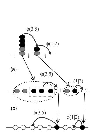
Figure 1: ZRP-ASEP (a) and particle-hole (b) transformations

Correspondingly, $m$ particles jumping from a site with $n$ particles to the next site are replaced by a one-step shift of an $m-$particle cluster detached from an $n-$particle cluster. The number of sites of the lattice in the ASEP-like system is equal to the number of sites in the ZRP-like system plus the number of particles.

The second duality is the particle-hole transformation, which relates two ASEP-like systems, Fig. 1(b). It interchanges the occupied and empty sites. A jump of a particle corresponds to a shift of the cluster of holes in the opposite direction. With this comment in mind we sketch a list of known models that can be obtained as limiting cases of our hopping probabilities (8).

Non-interacting particles, $q=1.$

It was noted above that the $q\to 1$ limit of the hopping probabilities gives us the binomial distribution. This corresponds to the free non-interacting particles, each performing the Bernoulli random walk independently of the others. That is to say that every time step all particles attempt to make jumps with the same probability $p$ given in (9). The binomial coefficient counts the number of ways to choose $m$ out of $n$ particles in a site. Note that taking the limit $q\to 1$ reduces the dependence on the two other parameters to a single parameter $p$. When $q\neq 1,$ the parameters $\nu$ and $\mu$ are responsible for an interaction between particles, which can be either repulsive or attracting, accelerating or deceleration the global motion. The Bernoulli random walks evolving with discrete time $t$ can be transformed into continuous time Poissonian random walks by taking limits $p\to 0$, i.e. $\mu\to\nu$, and $t\to\infty$ simultaneously, so that new continuous time $\tau=tp$ remains finite.

TASEP with generalized update, $q=0.$

In the ZRP picture particles jump from a site occupied by $n$ particles with probabilities $\varphi(0|n)=(1-p)$, $\varphi(m|n)=(1-\mu)p\mu^{m-1}$ for $0<m<n$ and $\varphi(n|n)=p\mu^{n-1}$. After ZRP-ASEP transformation this limit reproduces the process proposed in [28]. Consider a version of the TASEP, with backward sequential update, where a particle jumping to a site remembers whether this site was empty or occupied before the current time step. Specifically, during an update each cluster of particles is scanned from the rightmost to the leftmost particle. The first particle makes an attempt to jump forward with probability $p.$ In the case of success the second one tries to jump with probability $\mu$, generally different from $p$, and so do the third, forth e.t.c.. If eventually a particle has failed to jump, all the subsequent particles within the same cluster will stay with probability one. If $\mu=p,$ we obtain the usual TASEP with backward sequential update, while $\mu=0$ corresponds to the parallel update case. Within the range $0<\mu<1$ the effective interaction varies from repulsive to attractive, with the limit $\mu\to 1$ corresponding to particles sticking together. The limit $p\to 0$ is the continuous time version of the TASEP if $\mu\sim p$ and the continuous time fragmentation model when $\mu$ stays finite.

Multiparticle hopping asymmetric diffusion and long range hopping models, $\nu\to\mu=q$.

If in this limit, if we set $p=dt$, the hopping probabilities simplify to $\varphi(m|n)\simeq dt/[n]_{1/q}$, where the subscript $1/q$ indicates that the q-number deformation parameter is $q^{-1}$, rather than $q$. The model with similar hopping probabilities was first proposed in [21]. It, however, admitted particle jumps in both directions, and the asymmetry strength was rigidly bound to parameter $q$. Its generalization, where the asymmetry strength is unrelated to $n-$dependence of the hopping probabilities, was considered in [39]. Its totally asymmetric version is given by the limit under consideration. After ZRP-ASEP transformation we obtain the ASEP-like model, proposed in [18], where a particle pushes its right neighbouring particles to the right with the rate $r_{n}=1/[n]_{1/q}$, depending on the number $n-1$ of these particles. The model interpolates between the continuous time TASEP and the drop-push model [43], corresponding to the limits $q\to\infty$ and $q\to 0$ respectively.

q-bosonic ZRP, q-TASEP and asymmetric avalanche process, $\mu=q\nu$.

In this case the first q-Pochhammer symbol $(\nu/\mu;q)_{m}$ vanishes as soon as $m>1$. Therefore, only single particle jumps remain allowed. The process obtained is a discrete time ZRP, where one particle jumps from a site occupied by $n$ particles with probability $\varphi(1|n)=p\cdot[n]$. The corresponding integrable model, q-boson model, was first discovered in [40] in the language of the algebraic Bethe ansatz. Its Hamiltonian (continuous time) version was later discussed as an interacting particle model in [21]. It appeared again in [23], where the question addressed was: What are the most general hopping probabilities, which make the totally asymmetric continuous time ZRP model integrable? Later the discrete time model was obtained by addressing the same question to the discrete time ZRP [26]. Again, the continuous time model can be obtained from the discrete time one by taking the limit $p\to 0.$ For the discrete time model the parameters take their values in the range $|q|<1,0<p<1,$ while in the continuous time case $q$ can be any real number. In the latter case the limit $q\to\infty$ corresponds to the drop-push model, where a particle goes to the next vacant site on the right jumping over all its neighbors after exponentially distributed waiting time or, equivalently, pushes all its right neighbors one step to the right. After the ZRP-ASEP and particle-hole transformations the q-bosonic ZRP becomes so called q-TASEP, where $\varphi(1|n)$ is a probability for a particle to jump one step forward, given its headway is $n$. The q-TASEP appeared recently as a limiting case of the Macdonald process [41] and was used to study a semi-discrete polymer in a random media [42].

Another interesting continuous time limit of this model, the Asymmetric Avalanche Process (AAP) [22], is obtained in the limit $\nu\to 0$ and $|q|<1$. Setting $1-p=dt$ and going to a moving reference frame, which shifts one step to the right every time step, we obtain an ASEP-like model, where the transitions between particle configurations are described in terms of non-local avalanche dynamics. Specifically, in the moving frame the continuous time dynamics looks as follows. Starting from a configuration with at most one particle at every site any particle can jump to the left neighbouring site after exponentially distributed waiting time. If a particle meets another particle at the target site it can carry the latter along with itself to the next site on the left with probability $(1-[2])$ or leave it and go further alone. In general, if in course of the avalanche $n>1$ particles are found at the same site, either all $n$ particles go to the next site on the left with probability $(1-[n])$ or otherwise one particle stays and $(n-1$) particles go. Thus, at every step the number of particles in the avalanche can either decrease or increase by one or stay unchanged. The avalanche ends when one particle from a pair goes to an empty site. The discrete time avalanche dynamics is considered instant in the slow Poissonian time scale, so that the avalanches plays the role of transitions between ASEP-like particle configurations. The interest to this model was caused by the phase transition from intermittent to continuous flow, which takes place in the infinite system at critical value of the density of particles $\rho_{c}=1/(1-q).$ The $q=0$ limit of AAP is again the drop-push model, in which, however, the particles jump to the opposite direction with respect to the one mentioned above.

Geometric q-TASEP, $\nu=0.$

Very recently a preprint [44] by Borodin and Corwin appeared, where two version of discrete time TASEP were proposed. One of them is the so-called geometric q-TASEP, where a particle is allowed to jump forward to any vacant site between it and the next particle. The probability $p_{n,\mu}(l)$ of the jump length $l$ depending on the headway $n$ can be obtained from our $\varphi(l|n)$ by setting $\nu=0$. The process can be obtained from our model by making ZRP-ASEP and particle hole transformations. Note that the processes discussed in [44] were obtained as a reduction of the Macdonald process, and the technique was developed for a particular case of evolution with step initial condition. A question was also posed whether the Bethe ansatz technique is available to study the same problem, which would allow a consideration of other initial and boundary conditions. The present paper answers this question giving even more general form of hopping probabilities.

Other limiting cases of our model can be considered, for which the hopping probabilities simplify. We mentioned those that appeared in the literature before. In addition, several models with partially asymmetric dynamics were proposed like the PASEP [2], two-parametric long range hopping model [19], multiparticle diffusion without exclusion [21], the Push-ASEP [45] and the AAP with two-sided hopping [46]. They can not be directly obtained as limiting cases of our totally asymmetric model. However, generality of the model makes us expect that being interpreted as a transfer matrix of a quantum integrable model our Markov matrix can generate also the Hamiltonians describing jumps in both directions, see e.g. [47].

3 Transfer matrix

We are going to find the conditions for the eigenproblem of the Markov matrix

$$\Lambda\mathbf{\Psi}=\mathbf{M}\mathbf{\Psi}$$

to be solvable by the Bethe ansatz. Here $\mathbf{M}$ is the matrix defined in (2,4), $\mathbf{\Psi}$ — a column vector, and $\Lambda$ is an eigenvalue. Our solution is based on the following observation. It is natural to expect that the groundstate, i.e. the eigenstate of the transfer matrix corresponding to the largest eigenvalue $\Lambda_{0}=1$, is the state of highest symmetry and, in particular, is translationally invariant. This is indeed the case for many models solved before. As the Bethe ansatz, which is supposed to give the eigenvectors, is an oscillating function, the groundstate Bethe vector should be zero momentum eigenstate, i.e. constant for all particle configurations. On the other hand, the groundstate of the chipping model with hopping probabilities of the form (4) is the product stationary state (3). However, the left eigenvector corresponding to the groundstate has exactly the required form $\bar{\mathbf{\Psi}}_{0}^{\mathbf{T}}=(1,\dots,1)$, where the superscript $\mathbf{T}$ refers to the matrix transposition transforming a column into a row. Therefore, we may try the Bethe ansatz to find the solution of the left eigenproblem.

$$\Lambda\bar{\mathbf{\Psi}}^{\mathbf{T}}=\bar{\mathbf{\Psi}}^{\mathbf{T}}\mathbf{M}$$

or equivalently

$$\Lambda\bar{\mathbf{\Psi}}=\mathbf{M^{T}}\bar{\mathbf{\Psi}}.$$

The key observation, first made in [48], is that the matrix $\mathbf{M}$ of the form (2,4) is related to its transpose $\mathbf{M^{T}}$ by simple conjugation

$$\mathbf{M^{T}=\Pi SMS^{-1}\Pi},$$ (10)

where $\mathbf{S}$ is the diagonal matrix with elements

$$S_{\mathbf{n,n^{\prime}}}=\delta_{\mathbf{n,n^{\prime}}}/P_{st}(\mathbf{n})$$

and $\mathbf{\Pi}$ is the parity transformation reversing the order of sites or equivalently the direction of motion. Indeed, consider matrix element $\mathbf{M_{n,n^{\prime}}}$ corresponding to the transition from a configuration $\mathbf{n}$ to a configuration $\mathbf{n^{\prime}}$. In fact, on a subset with fixed number of particles the sum in (2) consists of the only term

$$\mathbf{M_{n,n^{\prime}}}=P_{st}(\mathbf{n})^{-1}\prod_{i\in\mathcal{L}}v(m{}_{i})w(n_{i}-m_{i}),$$

where $m_{i}\geq 0$ is the number of particles jumping from site $i$ to site $(i+1)$. Once $\mathbf{n}$ and $\mathbf{n^{\prime}}$are given, the numbers $m_{i}$ can be uniquely determined from the system of equations

$$n_{i}-m_{i}=n^{\prime}_{i}-m_{i-1},\,i\in\mathcal{L}.$$ (11)

Only those matrix elements are nonzero, which yield non-negative $m_{i}$ for all $i\in\mathcal{L}$. Conjugation with matrix $\mathbf{S}$ affects the matrix elements of $\mathbf{M}$ by replacing the factor $P_{st}(\mathbf{n})^{-1}$ by $P_{st}(\mathbf{n}^{\prime})^{-1}$:

$$(\mathbf{SMS}^{-1})_{\mathbf{n,n^{\prime}}}=P_{st}(\mathbf{n^{\prime}})^{-1}\prod_{i\in\mathcal{L}}v(m{}_{i})w(n_{i}-m_{i}).$$ (12)

On the other hand, the matrix elements of $\mathbf{M^{T}}$, which can be thought of as transition weights of the time reversed process, are

$$(\mathbf{M^{T}})_{\mathbf{n,n^{\prime}}}=\mathbf{M_{n^{\prime},n}}=P_{st}(\mathbf{n^{\prime}})^{-1}\prod_{i\in\mathcal{L}}v(m^{\prime}{}_{i})w(n^{\prime}_{i}-m^{\prime}_{i}),$$ (13)

where $m^{\prime}_{i}=m_{i-1}$ is the number of particles one must transfer back to site $(i-1)$ from site $i$ to return from $\mathbf{n^{\prime}}$ to $\mathbf{n}$. Taking into account (11) and the translation symmetry of the lattice, we see that the weights (12) and (13) exactly coincide. The only difference is that in the time reversed process the particles move in the opposite direction.

Thus, we are going to solve the eigenproblem for matrix $\mathbf{M^{0}\equiv\mathbf{SMS}}^{-1}$, defined by matrix elements (12). Once its eigenvectors $\mathbf{\Psi^{0}}$ have been found, the right eigenvectors of $\mathbf{M}$ are $\mathbf{\mathbf{\Psi}}=\mathbf{S}^{-1}\mathbf{\Psi^{0}}$ and the left eigenvectors can be obtained by applying the parity transformation $\bar{\mathbf{\Psi}}=\mathbf{\Pi\Psi^{0}}$. Specifically, we are looking for functions $v(k)$ and $w(k)$ that ensure the Bethe ansatz solvability of the eigenproblem for $\mathbf{M^{0}}$.

Before going into calculations, we note that the hopping probabilities $\varphi(m|n)$ are invariant with respect to simultaneous transformations $v(k)\to a\theta^{k}v(k),\,\,w(k)\to b\theta^{k}w(k)$, where $a,b$ and $\theta$ are arbitrary nonzero constants. This three-parametric freedom can be removed by imposing three constraints on these functions. For example we can fix the functions $w(k)$ and $v(k)$ at three values of arguments (two for one of them and one for the other). Now we choose two of them as

$$v(0)=w(0)=1.$$ (14)

Thus, we fix the stationary weight of empty site, $f(0)=1$. Before fixing the third constraint we note that $\varphi(m|n)$ can be represented as a function of ratios $v(n)/(v(1))^{n}$ and $w(n)/(v(1))^{n}$ rather than on $v(n)$ and $w(n)$ alone. Therefore fixing the value of $v(1)$ is equivalent to fixing an exponential part of functions $w(k)$ and $v(k).$ This will be done in A, when we go to a more convenient parametrization.

We also should note that in general the stationary measure $P_{st}(\,)$ constructed as a product (3) is not normalized even in the finite system. If we want a probability measure, the overall normalization factor, called the partition function, must be evaluated.

As usual in the coordinate Bethe ansatz technique, we first consider the one-particle problem. Then, the two-particle problem looks as a direct product of one-particle problems in the range of particle coordinates, where the interaction is absent. The interaction, which reveals itself only at the border of physical domain of particle coordinates, can be accounted for as boundary conditions. Then, one has to consider many-particle problem with three and more particles on the lattice. The condition of the Bethe ansatz solvability is that all the many particle interactions are introduced via the two-particle boundary conditions.

One particle.

A representation of particle configurations equivalent to the one used above can be given in terms of positions of particles on the lattice. From now on we specify an $N-$particle configuration by a set of weakly increasing coordinates of particles

$$\mathbf{x}=(x_{1},\leq\dots,\leq x_{N}).$$ (15)

For one particle on the lattice the whole configuration is a single particle coordinate $x_{1}\equiv x$. Then the eigenproblem reads as follows

$$\Lambda_{1}\Psi^{0}(x)=p\Psi^{0}(x-1)+(1-p)\Psi^{0}(x),$$ (16)

where $p\equiv\varphi(1|1)=v(1)/(v(1)+w(1)).$ The corresponding stationary weights are $f(1)=v(1)+w(1).$ As we discussed above, the parameter $p$ depends only on the ratio $w(1)/v(1)$.

Two particles.

Now we have to consider the cases with two particles located at different sites, $x_{1}<x_{2}$, and at the same site, $x_{1}=x_{2}\equiv x$, separately. Inspecting the expression (12) of the matrix elements of $\mathbf{M^{0}},$ we find out that in the first case they depend on parameters of the dynamics via $p$ (i.e. via $w(1)/v(1)$) and, in fact, look like the two independent one-particle problems

$$\Lambda_{2}\Psi^{0}(x_{1,}x_{2}) = (1-p)[p\Psi^{0}(x_{1}-1,x_{2})+(1-p)\Psi^{0}(x_{1,}x_{2})],$$ (17)

$$+ p[p\Psi^{0}(x_{1}-1,x_{2}-1)+(1-p)\Psi^{0}(x_{1,}x_{2}-1)].$$

If this form was valid in the whole range of particle coordinates, there would not be any more complications comparing to the one-particle equation (16). In the case $x_{1}=x_{2}\equiv x$, however, the non-interacting form breaks up, and the new parameters $w(2)$ and $v(2)$ (in fact $w(2)/(v(1))^{2}$ and $v(2)/(v(1)){}^{2}$) come into the game

$$\Lambda_{2}\Psi^{0}(x,x)=f(2)^{-1}[w(2)\Psi^{0}(x,x)+v(1)w(1)\Psi^{0}(x-1,x)+v(2)\Psi^{0}(x-1,x-1)],$$ (18)

where $f(2)=w(2)+v(1)w(1)+v(2).$ To restore the free equation (17) let us formally rewrite it for the case $x_{1}=x_{2}\equiv x$. We notice that term $\Psi^{0}(x,x-1)$ appears, which is beyond the physical domain (15). In the following we refer to terms of this kind as forbidden and to those within the physical domain as allowed. It is our choice to assign the value to the forbidden term in such a way, that it compensates the difference between free equation (17) and interacting one (18).

$$\Psi^{0}(x,x-1)=\alpha\Psi^{0}(x-1,x-1)+\beta\Psi^{0}(x-1,x)+\gamma\Psi^{0}(x,x),$$ (19)

where

$$\alpha=\frac{v(2)/f(2)-p^{2}}{p(1-p)},\,\beta=\frac{v(1)w(1)/f(2)}{p(1-p)}-1,\,\gamma=\frac{w(2)/f(2)-(1-p)^{2}}{p(1-p)}.$$ (20)

The equation (17) supplied with the boundary conditions (19) completely define the two-particle problem.

$N$ particles.

For arbitrary number of particles the equations should in principle include all the parameters $w(n)$ and $v(n)$ for $n=1,\dots,N,$ which generally can be arbitrary. The integrability, however, restricts the choice. To make the problem solvable we try to represent our equations as the equations for non-interacting particles with suitable boundary conditions in the same vein as we did for the two-particle case. The basic condition of the Bethe ansatz solvability is all the boundary conditions being of the same form (19). This fact reduces the set of independent parameters to those three we have already used.

An example of the procedure for three particles, $N=3$, is as follows. First, when we write down the equations for three particles with $\Lambda_{3}\Psi^{0}(x_{1},x_{2},x_{3})$ in the l.h.s., we find three different cases to be considered: three particles in different sites, i.e. $x_{1}<x_{2}<x_{3}$, one particle in one site and two in another, $x_{1}=x_{2}<x_{3}$ or $x_{1}<x_{2}=x_{3},$ and all the three particles in the same site, $x_{1}=x_{2}=x_{3}\equiv x$. The first case, is already the equation for three independent particles. The second one is a combination of one- and two-particle problems, (16) and (18), which can be converted to the non-interacting form by applying the two-particle boundary conditions (19) to the pairs of coordinates in inverse order, e.g. $(x,x-1)$. An essentially new case is the equation with $\Psi^{0}(x,x,x)$ in the l.h.s.. Again, we would like to replace it by the equation for three independent particles. If we write corresponding non-interacting equation, it will contain four forbidden terms in the r.h.s: $\Psi^{0}(x,x,x-1)$, $\Psi^{0}(x,x-1,x-1)$, $\Psi^{0}(x,x-1,x)$ and $\Psi^{0}(x-1,x,x-1).$ The idea is to express them in terms of the allowed configurations only using the boundary conditions of the form (19). Note that if we simply apply our boundary conditions to the pairs of coordinates $(x,x-1)$, some of the terms we obtain will be forbidden again. However, they will be found among the four terms we have just mentioned. In fact, the relations we will obtain in this way can be treated as the system of four linear equations for four forbidden terms, which, having been solved, yields the forbidden terms expressed via the allowed terms. The solution must be substituted into the non-interacting equation, so that only the allowed terms remain. Then, we compare the coefficients coming with the allowed terms with the coefficients in the true interacting equation and try to identify the values of $v(3)$ and $w(3)$, relying on the expectation that the solution for the hopping probabilities of the suggested form (4) exists.

The procedure for arbitrary $N$ is similar. We want to transform the equation for non-interacting particles to the equation for interacting particles using the two-particle boundary conditions. Remarkably, the transformation we did to the transition matrix resulted in the transition coefficients, which factorize into a product of single-site terms, which depend only on the number of particles coming to a site and on the number of particles in this site after the transition. To illustrate this fact consider the transition in which site $x$ becomes occupied by $n$ particles after $k$ particles have arrived from site $(x-1)$ and some particles may have jumped out. The $k$ particles that have jumped in bring the factor $\nu(k)$, while those $(n-k)$ that have stayed bring the factor $w(n-k)$. The overall denominator is $f(n)$ independently of the previous state of the site. Therefore, the equation with $\Lambda\Psi^{0}(\dots,x^{n},\dots)$ in the l.h.s. will contain the sum

$$\sum_{k=0}^{n}\varphi(k|n)\Psi^{0}(\dots,(x-1)^{k},x{}^{n-k},\dots)$$ (21)

on the right, where $x^{n}$ means a string of $n$ letters $x$, i.e. $n$ particles in the site $x$ and the coefficients are supposed to be of the form $\varphi(n|k)=v(k)w(n-k)/f(n)$, the same as in (4). For several occupied sites we have products of similar terms summed independently of each other. The corresponding part of the non-interacting equation is

$$\sum_{k_{1}=0}^{1}\dots\sum_{k_{n}=0}^{1}p^{k_{1}+\dots+k_{n}}(1-p)^{n-(k_{1}+\dots+k_{n})}\Psi^{0}(\dots,x-k_{1},\dots,x-k_{n},\dots).$$ (22)

Our aim is to reduce one equation to the other by iterative application of the two-particle boundary conditions. As a result we will get the arguments of all terms $\Psi^{0}(\,)$ ordered so that all the symbols $(x-1)$ appear on the left of the symbols $x$.

3.1 Generalized quantum binomial

The problem can be formalized as that of the generalized quantum binomial. Consider an associative algebra generated by two elements $A$ and $B$, which obey a general homogeneous quadratic relation

$$BA=\alpha AA+\beta AB+\gamma BB.$$ (23)

Within the set of all words made of the symbols $A$ and $B$ we distinguish a subset of normally ordered words, where all symbols $A$ are put on the left of all symbols $B$, i.e. where no combination $BA$ is present. An arbitrary homogeneous element of the algebra can be represented as a linear combination of normally ordered words of the same degree, obtained by repetitive application of the relation (23). That this representation is unique is guaranteed by the diamond lemma [49]. A particularly interesting example of the normally ordered representation is a non-commutative analogue of the Newton binomial:

$$(A+B)^{n}=\sum_{0\leq k\leq n}\mathcal{C}_{k}^{n}A^{k}B^{n-k},$$ (24)

where $\mathcal{C}_{k}^{n}$ are the generalized binomial coefficients depending on the parameters of the defining relation. In purely commutative case, $\alpha=\gamma=0,\,\beta=1$, and in the case of $q-$commuting variables , $\alpha=\gamma=0,\,b=q,$ $\mathcal{C}_{k}^{n}$ are well known to be the usual binomial and the $q-$binomial coefficients, respectively. We are interested in the case of generic coefficients $\alpha,\beta,\gamma.$ Indeed, let us associate $A$ with $(x-1)$ and $B$ with $x$ in (21, 22). The boundary conditions (19) used to get rid of the forbidden combinations $(\dots,x,x-1,\dots)$ act just like the defining relations (23). What we need is to construct the following “skew” binomial sum

$$(pA+(1-p)B)^{n}=\sum_{m=0}^{n}\varphi(m|n)A^{m}B^{n-m},$$ (25)

where coefficients $\varphi(n|k)$ are nothing but the jumping probabilities to be defined. In principle, instead of defining the parameters $\alpha,\beta,\gamma$ in terms of one and two particle dynamics, we could go the other way around, starting from assigning them any complex values considered as input data. The resulting coefficients $\varphi(n|m)$ would define the matrix $\mathbf{M}^{0},$ which is still diagonalizable by the Bethe ansatz. Then, however, the problem might lose its probabilistic content, though possibly could still be treated as some quantum or statistical physics model. In our case the values of $\alpha,\beta,\gamma$ read from (20) satisfy relation $\alpha+\beta+\gamma=1,$ which remove one degree of freedom. On the other hand, the parameter $p$ in the l.h.s. of (25) yields another degree of freedom, so that we again have three free parameters, e.g. $v(2)$, $w(2)$ and $p$ or $w(1).$ Note that (25) can be reduced to (24) by absorbing the parameter $p$ into $A$ and/or $B$ and changing the defining relations accordingly, which return us to the generic case. Also, the range of the values of $\alpha,\beta,\gamma$ is limited by the condition that the coefficients $\varphi(n|k)$ have the meaning of hopping probabilities, i.e. $v(n)\geq 0$ and $w(n)\geq 0$ for any $n\geq 0.$ As we do not know whether the generalized binomial formula for the case of generic homogeneous quadratic relations appeared in the literature before, we state it as a theorem. The expression of the generalized binomial coefficients (aka hopping probabilities $\varphi(m|n)$ ) is a main result of the present paper. The proof of this theorem is brought to A.

Theorem 1.

Consider an associative algebra over complex numbers with two generators $A$,$B$. Suppose the generators satisfy the homogeneous quadratic relation (23), where $\alpha,\beta,\gamma$ are arbitrary complex numbers constrained by $\alpha+\beta+\gamma=1.$ Then, for any complex number $p,$ the coefficients $\varphi(m|n)$ of the binomial sum (25) are given by the formula (8), where $q,\nu$ and $\mu$ give a convenient parametrization for $\alpha,\beta,\gamma$ and $p$:

$$\alpha=\frac{\nu(1-q)}{1-q\nu},\,\beta=\frac{q-\nu}{1-q\nu},\,\gamma=\frac{1-q}{1-q\nu}$$ (26)

and

$$\mu=p+\nu(1-p),$$ (27)

and we suppose that $\nu\neq q^{-k}$, for any $k\in\mathbb{N}.$

One can see that $\varphi(m|n)$ has indeed the product form (4). For $n=2$ it complies with the definition (20).

4 Bethe ansatz

Now we are in a position to diagonalize the matrix $\mathbf{M}^{0}$. The eigenproblem is reformulated as the free equation

$$\Lambda_{N}\Psi^{0}(\mathbf{x})=(1-p)^{n}\sum_{\mathbf{k}\in\{0,1\}^{\otimes N}}\left(\frac{p}{1-p}\right)^{||\mathbf{k}||}\Psi^{0}(\mathbf{x}-\mathbf{k}),$$ (28)

where $||\mathbf{k}||=k_{1}+\dots+k_{N}$, supplied with the boundary conditions

$$\Psi^{0}(\dots,x,x-1,\dots) = \alpha\Psi^{0}(\dots,x-1,x-1,\dots)$$

$$+ \beta\Psi^{0}(\dots,x-1,x,\dots)+\gamma\Psi^{0}(\dots,x,x,\dots),$$ (29)

where the parameters $\alpha,\beta,\gamma$ are given in (26) expressed in terms of $q$ and $\nu$. We are looking for an eigenfunction in form of the Bethe ansatz

$$\Psi^{0}(\mathbf{x|z})=\sum_{\sigma\in S_{N}}A_{\sigma}\hat{\sigma}\mathbf{z}{}^{\mathbf{x}},$$ (30)

that depends on $N-$tuple of “quantum” numbers $\mathbf{z}=(z_{1},\dots,z_{N}).$ Here the summation is performed over the set $S_{N}$ of all permutations $\sigma=(\sigma_{1},\dots,\sigma_{N})$ of the numbers $1,\dots,N$, the hat symbol indicates the action of an element of the permutation group on the functions of $N-$tuple $\mathbf{z}$, $\hat{\sigma}\mathbf{z}=(z_{\sigma_{1}},\dots,z_{\sigma_{N}})$ and $\hat{\sigma}\mathbf{z^{x}}=(z_{\sigma_{1}}^{x_{1}},\dots,z_{\sigma_{N}}^{x_{N}})$, and $A_{\sigma}$ are the coefficients to be defined, indexed by permutations. Substituting this ansatz into the equation (28) we obtain the eigenvalue as a function of the parameters $\mathbf{z}$,

$$\Lambda_{N}(\mathbf{z})=\prod_{i=1}^{N}\Lambda_{1}(z_{i}),$$ (31)

which is a product of one-particle eigenvalues

$$\Lambda_{1}(z)=1-p+p/z.$$ (32)

The boundary conditions yield the S-matrix, the ratio of two coefficients $A_{\sigma}$ corresponding to permutations differing from each other in an elementary transposition of two neighbors,

$$S(z_{i},z_{j})\equiv\frac{A_{\dots ij\dots}}{A_{\dots ji\dots}}=-\frac{\alpha+\beta z_{i}+\gamma z_{i}z_{j}-z_{j}}{\alpha+\beta z_{i}+\gamma z_{i}z_{j}-z_{j}}.$$ (33)

Given the initial condition $A_{id}=1$ for the identical permutation $id=(1,\dots,N)$, this can be solved to

$$A_{\sigma}=\mathrm{sgn}(\sigma)\prod_{1\leq i<j\leq N}\frac{\alpha+\beta z_{\sigma_{i}}+\gamma z_{\sigma_{i}}z_{\sigma_{j}}-z_{\sigma_{j}}}{\alpha+\beta z_{i}+\gamma z_{i}z_{j}-z_{j}},$$ (34)

where $\mathrm{sgn}(\sigma)$ is the permutation sign.

To write the above formulas in a shorter form we make a variable change

$$z_{i}=\frac{1-\nu u_{i}}{1-u_{i}}.$$ (35)

Then, the $S$-matrix simplifies to

$$S(u,v)=\frac{qv-u}{v-qu},$$ (36)

the form familiar from studies in quantum integrable systems, and the one-particle eigenvalue in new variables looks as follows

$$\Lambda_{1}(u)=\frac{1-\mu u}{1-\nu u}.$$ (37)

Hence we have

$$\Lambda_{N}=\prod_{i=1}^{N}\left(\frac{1-\mu u_{i}}{1-\nu u_{i}}\right),$$ (38)

and the components of the eigenvector of $\mathbf{M}^{0}$are

$$\Psi^{0}(\mathbf{x}|\mathbf{z})=\sum_{\sigma\in S_{N}}\mathrm{sgn}(\sigma)\prod_{i=1}^{N}\prod_{\begin{array}[]{c}j>i\end{array}}\frac{u_{\sigma_{i}}-qu_{\sigma_{j}}}{u_{i}-qu_{j}}\frac{\left(1-\nu u_{\sigma_{i}}\right)^{x_{i}}}{\left(1-u_{\sigma_{i}}\right)^{x_{i}}}.$$ (39)

This is used to write the right and left eigenvectors of $\mathbf{M}$, which, according to the discussion in the beginning of the section, are obtained by maltiplying $\Psi^{0}(\mathbf{x}|\mathbf{z})$ by $P_{st}(\mathbf{x})$ and by applying parity transformation to the spacial coordinates respectively:

$$\Psi(\mathbf{x}|\mathbf{z})\sim P_{st}(\mathbf{x})\Psi^{0}(\mathbf{x}|\mathbf{z}),\,\,\,\bar{\Psi}(\mathbf{x|}\mathbf{z})\sim\Psi^{0}(\mathbf{\hat{\Pi}x}|\mathbf{z}).$$ (40)

Here, the result of the action of parity transformation applied to $\Psi^{0}(\mathbf{x}|\mathbf{z})$ is replacement of particle coordinates $x_{i}$ to $-x_{i}$ and, correspondingly, inverting the order of particles $i\to N-i+1$, i.e. $\hat{\Pi}\mathbf{x}=(-x_{N},\dots,-x_{1})$. Note that the proportionality sign “$\sim$” reflects the fact that the components of eigenvectors are defined up to an arbitrary $\mathbf{z}$-dependent factor, which can be fixed by normalization conditions.

The spectrum of parameters $\mathbf{z}$ depends on the type of the lattice. The infinite lattice and the ring should be considered separately.

4.1 Infinite lattice and Green function conjecture

On the infinite lattice the parameters $\mathbf{z}$ can take any values. In practice, what we want is to use the eigenfunctions to expand the solutions of the master equation with given initial conditions. Specifically, the eigenvectors of the matrix $\mathbf{M}$ can be used as an analogue of the Fourier basis. Given the probability distribution $P_{t}(\mathbf{x})$ we would like to represent it as an integral

$$P_{t}(\mathbf{x})=\int\tilde{P}_{t}(\mathbf{z})\Psi(\mathbf{x}|\mathbf{z})\mathcal{M}(d\mathbf{z}),$$ (41)

where the measure $\mathcal{M}(\,)$ and the domain of integration have to be chosen consistent with initial conditions. Given a function $\tilde{P}_{0}(\mathbf{z})$ that provides the integral representation at time $t=0$, the time dependence of the Fourier coefficients directly follows from the fact that $\Psi(\mathbf{x}|\mathbf{z})$ is an eigenvector of the matrix $\mathbf{M}$:

$$\tilde{P}_{t}(\mathbf{z})=\left[\Lambda_{N}(\mathbf{z})\right]^{t}\tilde{P}_{0}(\mathbf{z}).$$

The choice of the measure and the domain of integration is verified by examining a particular case of the initial conditions, $P_{0}(\mathbf{x})=\delta_{\mathbf{x,x^{0}}}$, while the other initial distributions can be considered as linear combinations of delta functions. In this case the Fourier coefficient $\tilde{P}_{0}(\mathbf{z})$ is expected to be proportional to $\bar{\Psi}(\mathbf{y|}\mathbf{z})$, the component of the left eigenvector of the matrix $\mathbf{M}$, while the relation (41) at $t=0$ follows from the generalized completeness relation:

$$\int\bar{\Psi}(\mathbf{y|}\mathbf{z})\Psi(\mathbf{x}|\mathbf{z})\mathcal{M}(d\mathbf{z})=C_{N}\delta_{\mathbf{x},\mathbf{y}},$$ (42)

where $C_{N}$ is a normalization constant. Using (40) we write the relation in the following form

$$\int\Psi^{0}(\mathbf{\hat{\Pi}y}|\hat{R}\mathbf{z})\Psi^{0}(\mathbf{x}|\mathbf{z})\mathcal{M}(d\mathbf{z})=\frac{C_{N}\delta_{\mathbf{x},\mathbf{y}}}{P_{st}(\mathbf{x})},$$ (43)

where $\hat{\Pi}\mathbf{y}=(-y_{N},\dots,-y_{1})$, and $R\mathbf{z}=(z_{N},\dots,z_{1})$. Correspondingly, given the system has started from a particle configuration $\mathbf{x^{0}}$, the probability distribution at arbitrary time, referred to as Green function in this case , is

$$G_{t}(\mathbf{x}|\mathbf{x^{0}})=C_{N}^{-1}P_{st}(\mathbf{x}^{0})\int\Lambda_{N}^{t}(\mathbf{z})\Psi^{0}(\mathbf{\hat{\Pi}x}^{0}|\hat{R}\mathbf{z})\Psi^{0}(\mathbf{x}|\mathbf{z})\mathcal{M}(d\mathbf{z}).$$ (44)

Our goal is to choose the integration measure and the domain, such that the relation (42) holds.

The solution was first proposed in [51] for the case of continuous time TASEP. Later this program was completed for a few models. In all the cases considered to date the integration is performed along the product of $N$ identical contours $\Gamma_{1}\times\dots\times\Gamma_{N}$ defined by rules of going around singularities of the integrand, and the measure is $\mathcal{M}(d\mathbf{z})=\bigwedge_{i=1}^{N}dz_{i}/(2\pi\mathrm{i}z_{i})$.

For the TASEP and drop-push models, which corresponds to $q=0,\infty$ of our model, the $S$-matrix possesses special factorization property $S(u,v)=g(u)/g(v)$, with a rational function $g(u).$ As a result the function $\Psi^{0}(\mathbf{x}|\mathbf{z})$ has determinantal form. The integrations in different variables decouple, and the integral is evaluated explicitly to a determinant of the matrix $N\times N$. In the simplest cases of the continuous time TASEP and the drop-push model, whose stationary measure is trivial, this matrix is upper triangular with the diagonal elements equal to one. A little more complicated case is the discrete time TASEP with the generalized [28] and, in particular, parallel update [48], where the stationary measure is not uniform. Then the integral evaluates to a determinant of a block diagonal matrix, which yields exactly the inverse stationary measure. In all these cases the Green function (44) is the determinant of an $N\times N$ matrix.

The situation is far more complicated when the $S$-matrix can not be factorized into a product of one variable functions.In this case, the poles of the integrand relate different variables to each other; a fine account of their contributions is necessary to prove the formulas (42-44). This was first implemented for the PASEP by Tracy and Widom [9], who used this result as a starting point of the derivation of the current distribution. Later, analogous proofs were given for several other models: the two-sided PushASEP, the asymmetric zero range process with uniform hopping rates, the asymmetric avalanche process [52] and the multiparticle hopping asymmetric diffusion model [39].

In our case, an explicit substitution of $\Psi^{0}$ to (43) yields two independent sums over permutations $\sigma$ and $\sigma^{\prime}$. By changing the summation variable in one of the sums to $\sigma^{\prime\prime}=\sigma\cdot\sigma^{\prime}$, one sum becomes trivial and we arrive at the conjecture

$$\sum_{\sigma\in S_{N}}\mathrm{sgn}(\sigma)\oint_{\Gamma_{1}^{0,\nu}}\dots\oint_{\Gamma_{N}^{0,\nu}}\prod_{i=1}^{N}\left(\prod_{j>i}\frac{\alpha+\beta z_{\sigma_{i}}+\gamma z_{\sigma_{i}}z_{\sigma_{j}}-z_{\sigma_{j}}}{\alpha+\beta z_{i}+\gamma z_{i}z_{j}-z_{j}}\right)$$

$$\,\hskip 56.9055pt\hskip 56.9055pt\times\frac{z_{\sigma_{i}}^{x_{i}-y_{\sigma_{i}}-1}dz_{i}}{2\pi\mathrm{i}}=\frac{N!C_{N}}{P_{st}(\mathbf{x})}\delta_{\mathbf{x},\mathbf{y}}.$$

Similarly to [48] we expect that the contours must encircle the poles of the integrand at $z_{i}=0,\nu$ leaving $z_{i}=1$ and $z_{i}=\infty$ outside. The normalization coefficient $C_{N}$ must be chosen such that the states with all particles being at different sites are normalized to one. Therefore

$$C_{N}=f(1)^{N}/N!.$$

With the use of new variables (35) our conjecture takes the following form.

Conjecture 2.

Let $|q|<1$ and $|\nu|<1$. Given two arbitrary $N-$tuples of integers $\mathbf{x}=(x_{1}\leq\dots\leq x_{N})$ and $\mathbf{y}=(y_{1}\leq\dots\leq y_{N})$, such that

$$y_{1} = \dots=y_{n_{1}},$$

$$y_{n_{1}+1} = \dots=y_{n_{1}+n_{2}},$$

$$\vdots$$

$$y_{n_{1}+n_{2}+\dots+1} = \dots=y_{N},$$

the following identity holds:

$$\sum_{\sigma\in S_{N}}\mathrm{sgn}(\sigma)\oint_{\Gamma_{1}^{0,1}}\dots\oint_{\Gamma_{N}^{0,1}}\prod_{i=1}^{N}\left(\prod_{\begin{array}[]{c}j>i\end{array}}\frac{u_{\sigma_{i}}-qu_{\sigma_{j}}}{u_{i}-qu_{j}}\right)$$ (47)

$$\,\,\,\,\,\,\times\frac{\left(1-\nu u_{\sigma_{i}}\right)^{x_{i}-y_{\sigma_{i}}-1}}{\left(1-u_{\sigma_{i}}\right)^{x_{i}-y_{\sigma_{i}}+1}}\frac{du_{i}}{2\pi\mathrm{i}}=\delta_{\mathbf{x},\mathbf{y}}(1-q)^{-N}\prod_{\{n_{i}\}}\frac{(q;q)_{n_{i}}}{(\nu,q)_{n_{i}}},$$ (48)

here the integration in $u_{1},\dots,u_{N}$ is performed along the contours $\Gamma_{1}^{0,1},\dots,\Gamma_{N}^{0,1}$ encircling the poles of the integrand at $u_{i}=0,1$ and leaving other poles outside.

We have checked the above statement for $N=2$ and leave it a conjecture for arbitrary $N$, since its proof requires some analytical effort and is beyond the goals of this paper. The condition $|\nu|<1$ guarantees that the contours $\Gamma_{i}^{0,1}$ can be chosen being circles of the radii $1<R<1/\nu$. For larger absolute values of $\nu$ one has to use the contours deformed accordingly. The condition $|q|<1$ ensures that the poles of the scattering matrix, corresponding to bound states, do not contribute into the integral. In the case $|q|>1$, where the bound states are important, they should be taken into account explicitly. In particular, in the case of the multiparticle hopping asymmetric diffusion model [39] the completeness relation required contours to have a special nested structure.

Given conjecture (48), the expression for the Green function is straightforward

$$G_{t}(\mathbf{x}|\mathbf{y}) = \left(1-q\right)^{N}\prod_{\{n_{i}\}}\frac{(\nu;q)_{n_{i}}}{(q,q)_{n_{i}}},\sum_{\sigma\in S_{N}}\mathrm{sgn}(\sigma)\oint_{\Gamma_{1}^{0,1}}\dots\oint_{\Gamma_{N}^{0,1}}$$

$$\prod_{i=1}^{N}\left(\prod_{\begin{array}[]{c}j<i\end{array}}\frac{u_{\sigma_{i}}-qu_{\sigma_{j}}}{u_{i}-qu_{j}}\right)\left(\frac{1-\mu u_{i}}{1-\nu u_{i}}\right)^{t}\frac{\left(1-\nu u_{\sigma_{i}}\right)^{x_{i}-y_{\sigma_{i}}-1}}{\left(1-u_{\sigma_{i}}\right)^{x_{i}-y_{\sigma_{i}}+1}}\frac{du_{i}}{2\pi\mathrm{i}}$$

where the numbers $n_{i}$ are defined as in (2).

4.2 Discrete spectrum on the ring

For the case of the ring the periodic boundary conditions on the eigenfunctions are imposed

$$\Psi(x_{1},\dots,x_{N}|\mathbf{z})=\Psi(x_{2},\dots,x_{N},x_{1}+L|\mathbf{z}).$$

A direct substitution of (30,33) gives

$$z_{i}^{L}=\prod_{i\neq j}S(z_{i},z_{j}),$$ (50)

where the S-matrix is given in (33). To write down the periodicity conditions explicitly we again use the variable change (35). In these variables we obtain the following Bethe ansatz equations:

$$\left(\frac{1-\nu u_{i}}{1-u_{i}}\right)^{L}=(-1)^{N-1}\prod_{j=1}^{N}\frac{u_{i}-qu_{j}}{u_{j}-qu_{i}},\,\,\,i=1,\dots,N.$$

The solutions of these equations are to be substituted into the eigenvalues and eigenvectors (38-40). These equations, the eigenvalues and the eigenvectors have appeared and been studied before in [26], where the particular case our model, discrete time q-ZRP, was discussed. There, however, the parameters $p,q$ and $\nu$ ($-\lambda$ of [26]) were related by the constraint $\nu=-p/(1-p-q)$, while here they can be considered as three independent quantities.

4.3 ZRP-ASEP transformation

It was mentioned above that one can construct an ASEP-like process by replacing a site with $n$ particles by a string of $n$ sites, occupied by one particle each, plus one empty site ahead. Correspondingly, the jump of $m$ particles from a site with $n$ particles will be replaced by a unit right step made by a cluster of $m$ particles detaching from the right end of an $n$-particle cluster. Technically, the transformation suggests that the coordinates of particles are transformed as

$$(x_{1},\dots,x_{N})\to(x_{1}+1,\dots,x_{N}+N),$$ (51)

and $N$ extra sites are added to the lattice $L\to L+N$. This is enough to establish a direct correspondence between finite time realizations of the processes.

This transformation can also be translated into the language of the Bethe ansatz. In the case of the ASEP-like dynamics the physically allowed domain of coordinates is defined by strict inequalities

$$x_{1}<\dots<x_{n}.$$ (52)

The equations for $\Psi^{0}(x_{1},\dots,x_{N})$ look as the one for non-interacting particles within this domain, while the interaction is set in by imposing the boundary conditions, which express the forbidden terms like $\Psi^{0}(\dots,x,x,\dots)$ via the allowed ones

$$\Psi^{0}(\dots,x,x,\dots) = \alpha\Psi^{0}(\dots,x-1,x,\dots)$$

$$+ \beta\Psi^{0}(\dots,x-1,x+1,\dots)+\gamma\Psi^{0}(\dots,x,x+1,\dots).$$ (53)

Again, the eigenvector has the form (30) of the Bethe ansatz, which yields the same formula (31) for the eigenvalue. Substituted into the boundary conditions it gives

$$\frac{A^{ASEP}_{\dots ij\dots}}{A^{ASEP}_{\dots ji\dots}}\equiv-\frac{z_{i}}{z_{j}}S(z_{i},z_{j}),$$

where $S(z_{i},z_{j})$ is the $S-$matrix (33) obtained for the ZRP-like dynamics. It is not difficult to see that the eigenfunction $\Psi^{0}(\mathbf{x}|\mathbf{z})$ defined as the Bethe ansatz with the coefficients $A_{\sigma}^{ASEP}$, is nothing but that obtained for ZRP expressed via the new coordinates of the particles in the ASEP-like system. This obviously leads to the same, up to a simple coordinate change, Green function as before.

A slight difference appears in the case of the finite ring. In this case the ZRP-ASEP transformation gives us one-to-one correspondence of the realizations of the processes (the sequence of particle jumps), while the particle configurations on the lattice are equivalent only up to a shift: when a particle in the ZRP makes the full rotation around the lattice restoring an original configuration, the corresponding TASEP configuration must be shifted one step back. This correspondence should also be translatable to the language of eigenvectors and eigenvalues, i.e. given the set of solutions of one system of the Bethe equations, we should reconstruct the solutions for the other, which, being substituted into the eigenvectors and eigenvalues, would provide the equivalence of the time evolutions. This correspondence, however, is hidden in symmetries of the Bethe equations and in the properties of the eigenfunctions constructed out of their solutions, and making it explicit is not a straightforward task.

In particular, the dimensions of the state spaces, i.e. the total numbers of particle configurations, are different, being $C_{L+N}^{N}$ for the ASEP-like systems and $C_{L+N-1}^{N}$ for the ZRP-like ones. These should be the multiplicities of the solutions of the Bethe equations, as every eigenvector corresponds to a unique solution (provided that all the eigenvectors are linearly independent). Imposing the periodic boundary conditions $\Psi(x_{1},\dots,x_{N}|\mathbf{z})=\Psi(x_{2},\dots,x_{N},x_{1}+L+N|\mathbf{z})$ on the lattice of the size $L+N,$ we arrive at the system of the Bethe equations for the TASEP-like system,

$$z_{i}^{L}\prod_{k=1}^{N}z_{k}=\prod_{i\neq j}S(z_{i},z_{j})\,\,\,,i=1,\dots,N$$ (54)

which differs from (50) by the factor $\theta=z_{1}\dots z_{N}$ in the l.h.s.. Taking products of all equations in (50) and in (54), we obtain $\theta^{L}=1$ and $\theta^{L+N}=1$ respectively. Let us use the variable $\theta$ instead of $z_{N}$, leaving the other $N-1$ variables unchanged. Obviously the equation for $\theta$ suggests that it takes $L$ and $L+N$ values for the ZRP and ASEP cases respectively. Given $\theta$ fixed, the other $N-1$ equations have similar, up to the factor $\theta$ in the l.h.s., structure in the two cases. Supposedly the multiplicities of their solutions are the same. Hence the ratio of the total numbers of solutions is $L/(L+N)$, which indeed must be the case. Of course, the rigorous proof of this fact requires more elaborate arguments, and so do the the proof of the full correspondence.

5 Conclusion

To summarize, we have found the three-parametric family of hopping probabilities for the class of chipping modes with on-site interaction, which, first, ensure the factorization of the stationary measure on the infinite lattice and on the ring, and, second, define a Markov matrix being a transfer matrix of an integrable model solvable by the Bethe ansatz. Our model contains most of models known to date as particular limiting cases. We also have given an interpretation of the model obtained by the ZRP-ASEP transformation in terms of the ASEP-like systems either with simultaneous jumps of clusters of particles or with long range single-particle jumps governed by long-range interactions.

We have constructed the Bethe ansatz solution for the infinite lattice and for the ring. In the former case we have formulated the conjecture on the form of Green function. If it is proven, the Green function could be used as a starting point for calculation of the distribution of the distance traveled by a tagged particle and, potentially, of the many-particle correlation functions. Nowadays we have a few examples of solutions of the former problem for different models and several types of initial conditions. The solution of the latter one is still an open question.

For the ring we obtained the eigenvectors in terms of solutions of the system of Bethe equations. This system can be explicitly solved in very few cases, mostly in the thermodynamic limit. Some results for infinite time limit can be obtained analogously to [2, 4, 3]. The most interesting task is search for correlation functions at finite time, which would provide us with an information about KPZ-specific crossover from the results obtained for infinite systems to finite size behaviour. General correlation functions of the integrable models on a ring is a long-standing challenging problem having a big history. Some steps in this direction for stochastic particle models have recently been done. However, a final solution to this problem has not yet been given.

In the present paper we limited ourselves by considering structural elements responsible for integrability and did not study the physics of the model. We expect that the scaling behaviour of the fluctuations of particle current on the infinite lattice will be similar to that of other models of KPZ class in the most part of the parameter space. There are however points in this space where particles either stick together and move as a single particle or become independent of each other. It is of interest to study the crossover regimes between KPZ behaviour and these points to find out how universal they are. Also the KPZ universality may break down at the point where the particle current loses its convexity as a function of the particle density. Whether the particle current in our model have any special points like that is yet to be studied.

When the article was ready to submission we came to know about a new work [53], where an elegant Plancherel theory was developed for the continuous time q-ZRP model. Among the results, there is a proof of our Conjecture 2 about completeness of the Bethe ansatz on the infinite lattice, completed for $\mu=q\nu,\nu\to 0$ limit of our model. The method also exploited the relation between forward and backward dynamics, similar to relation (10) between the Markov matrix and its transpose. It is of interest to extend the technique of that paper to the case of three parameters.

In another article [54], appeared right after our article was submitted to the journal, the formula of the Green function for continuous time q-ZRP model was also proved, which was then used to obtain the integral representation for the distribution of the left-most particle’s position.

Appendix A Proof of Theorem 1.

We need to prove that given the generators $A$ and $B$ satisfying quadratic relation (23), the expansion (25) holds with the expansion coefficients (8),

$$\varphi(m|n)=\mu^{m}\frac{(\nu/\mu;q)_{m}(\mu;q)_{n-m}}{(\nu;q)_{n}}\frac{(q;q)_{n}}{(q;q)_{m}(q;q)_{n-m}},$$

where the parameters $q,\nu$ and $\mu$ parameterize $\alpha,\beta,\gamma$ and $p$ in accordance with (26,27). The proof is inductive. The statement obviously holds for $n=1$. Indeed, in this case $\varphi(0|1)=(1-\mu)/(1-\nu)=1-p$ and $\varphi(1|1)=(\nu-\mu)/(1-\nu)=p.$ We suppose that it is true for $n-1$ and prove it for $n$. Let us rewrite $(pA+(1-p)B)^{n}$ in form $(pA+(1-p)B)^{n-1}(pA+(1-p)B)$ and apply the expansion (8) to the first term

$$(pA+(1-p)B)^{n}=\sum_{m=0}^{n}\varphi(m|n-1)\left[pA^{m}B^{n-m-1}A+(1-p)A^{m}B^{n-m}\right].$$ (55)

To find $\varphi(n|m)$ we want the summands being normally ordered words. What violates the normal order is the factor $B^{n-m-1}A$. Thus we need to find expansion coefficients for the words of this kind.

Let us suppose that for any $l\geq 1,$ expansion

$$B^{l-1}A=\sum_{k=0}^{l}a_{k}^{l}A^{l-k}B{}^{k},$$ (56)

holds, where $a_{k}^{l}$ are the coefficients to be found. In particular, for $l=1,2$ we have

$$a_{0}^{1} = 1,a_{1}^{1}=0,$$ (57)

$$a_{0}^{2} = \alpha,a_{1}^{2}=\beta,a_{2}^{2}=\gamma.$$ (58)

With such defined $a_{k}^{l}$, we can rewrite (56) as

$$(pA+(1-p)B)^{n} = (1-p)\sum_{l=0}^{n-1}\varphi(l|n-1)A^{l}B^{n-l}$$

$$+p \sum_{l=0}^{n}\left[\sum_{m=0}^{l}\varphi(m|n-1)a_{n-l}^{n-m}\right]A^{l}B^{n-l},$$

which suggests

$$\varphi(l|n) = p\sum_{m=0}^{l}\varphi(m|n-1)a_{n-l}^{n-m}+(1-p)\varphi(l|n-1),\,\,\,l<n$$ (59)

$$\varphi(n|n) = p\sum_{m=0}^{n-1}\varphi(m|n-1)a_{0}^{n-m}$$ (60)

Therefore, before proceeding with finding, $\varphi(l|n)$ we first need to find coefficients $a_{m}^{n}$. To this end we note that the expansion (56) is a consequence of a successive application of the single relation (23). Therefore, the coefficients of interest satisfy a set of constraints. To write down the constraints let us represent $B^{l}A$ as $B^{l-1}(BA)$ and apply the relation (23) to the second factor.

$$B^{l}A = B^{l-1}(\alpha A^{2}+\beta AB+\gamma B^{2})$$

$$= \sum_{k=0}^{l}a_{k}^{l}(\alpha A^{l-k}B{}^{k}A+\beta A^{l-k}B{}^{k+1})+\gamma B^{l+1}$$

$$= \alpha\sum_{k=0}^{l}\sum_{j=0}^{k+1}a_{k}^{l}a_{j}^{k+1}A^{l-j+1}B{}^{j}+\beta\sum_{k=0}^{l}a_{k}^{l}A^{l-k}B^{k+1}+\gamma B^{l+1}$$

$$= \alpha\sum_{j=0}^{l+1}A^{l-j+1}B{}^{j}\left(\sum_{k=j-1}^{l}a_{k}^{l}a_{j}^{k+1}\right)+\beta\sum_{j=1}^{l+1}a_{j-1}^{l}A^{l-j+1}B^{j}+\gamma B^{l+1}$$

Here we used the expansion (56) applied to $B^{l-1}A$ in the second line and applied to $B{}^{k}A$ in the third line and then exchanged the summation order in the last line. Doing this we adopted a convention $a_{j}^{l}=0$ for $j<0$ and $l>0$. Collecting factors coming with $A^{l+1-j}B^{j}$ for $j=0,\dots,l+1$ and bringing the term containing $a_{j}^{l+1}$ to the l.h.s., we have

$$a_{j}^{l+1}=(1-\alpha a_{l}^{l})^{-1}\left(\alpha\sum_{k=j-1}^{l-1}a_{k}^{l}a_{j}^{k+1}+\beta a_{j-1}^{l}+\delta_{j,l+1}\gamma\right).$$ (61)

One can see that the set of relations has a triangular structure, i.e. $a_{j}^{l}$ can be expressed in terms of $a_{i}^{k}$ with $k\leq l$ and $k-i\leq l-j$ only. Therefore, we first can find $a_{i}^{l}$ with $l=i,$ then with $l=i+1$ e.t.c..

$a_{l}^{l}:$ The sum in the r.h.s. of (61) is empty and the relations are reduced to a simple recursion

$$a_{l+1}^{l+1}=\frac{\gamma+\beta a_{l}^{l}}{1-\alpha a_{l}^{l}}$$

with the initial condition $a_{1}^{1}=0$. This is a Riccati difference equation, which can be linearized by the variable change $a_{l}^{l}=1+\eta/c_{l},$ where $\eta$ is chosen such that the equation for $c(l)$ is linear. At this point it is more convenient to use the parameters $\nu$ and $q$ instead of $\alpha,\beta,\gamma$. In terms of these parameters we can choose either $\eta=1$ or $\eta=1/\nu$. Then we obtain two relations, which go into one another under the change $q\to 1/q$. Therefore, without loss of generality we choose $\eta=1/\nu$, which yields relation

$$c_{l+1}=qc_{l}-\frac{\nu(1-q)}{1-\nu}$$

subject to initial condition $c_{1}=-\nu.$ This recursion can be solved to

$$c_{l}=\frac{\nu(1-\nu q^{l-1})}{\nu-1},$$

which, after going back to $a_{l}^{l}$ yields the result

$$a_{l}^{l}=\frac{1-q^{l-1}}{1-\nu q^{l-1}}.$$

$a_{l}^{l+1}:$ The sum in the r.h.s. of (61) consists of a single term and we obtain

$$a_{l}^{l+1} = a_{l-1}^{l}\frac{\beta+\alpha a_{l}^{l}}{1-\alpha a_{l}^{l}}$$

$$=a_{0}^{1} \prod_{k=1}^{l}\frac{\beta+\alpha a_{k}^{k}}{1-\alpha a_{k}^{k}}$$

$$= \frac{q^{k}(q-\nu)(1-\nu)}{\left(1-\nu q^{k-1}\right)\left(1-\nu q^{k}\right)}.$$

We can make a few more steps in this way. At every step we obtain a linear recurrent relation that can be iterated and solved subject to the initial condition $a_{-1}^{l}=0.$ However, the calculations quickly become too involved. Fortunately, we can use the results of the first few steps to make an educated guess about general structure of $a_{k}^{l}$, which then can be proved by induction.

Lemma 3.

For $l>0$ and $k<l$ we have

$$a_{k}^{l}=(1-\nu)(q-\nu)\nu^{l-k-1}q^{k-1}\frac{(q;q)_{l-1}(\nu;q)_{k-1}}{(q;q)_{k}(\nu;q)_{l}}\,\,\,\mathrm{for}\,\,\,n>k$$ (62)

and

$$a_{l}^{l}=\frac{1-q^{l-1}}{1-\nu q^{l-1}}.$$ (63)

Proof.

It follows from (57,63) that the formulas (62,63) hold in the cases $l=1,2$. Suppose they also hold for $a_{j}^{l}$ for $l\leq n$ and $j\leq l$. To prove them for $l=n+1$ we substitute (62,63) into the r.h.s. of (61), which, after tedious but elementary algebra, yield the desired result. The main ingredient of the calculation is evaluation of the sum, which turns out to have a telescopic structure. ∎

Now we are in a position to complete the proof of the form of $\varphi(m|n).$ In fact, the principle a proof by induction simply requires that we substitute (8) into the r.h.s. of (59,60) and show that the l.h.s. also complies with this formula. This indeed what will finally be done. However, we first show some steps leading to a final formula and simplifying the problem to expressions, from which it can be guessed.

Let us use the ansatz (4),

$$\varphi(m|n)=\frac{v(m)w(n-m)}{f(n)},\,\,\,\mathrm{where}\,\,\,f(n)=\sum_{i=0}^{n}v(i)w(n-i),$$

which was the ansatz for the hopping probabilities that ensured the factorized structure of the stationary state. We recall that $v(m)$ and $w(m)$ are arbitrary positive valued function of $m,$ for which we have fixed $v(0)=w(0)=1,$ while another free parameter $v(1)$ can yet be fixed without loss of generality. Note that it is not obvious from eqs. (59,60) that $\varphi(m|n)$ must have this structure. However, once we have found the solution of this form, which complies with the initial conditions, an induction will provide its uniqueness. Let us write the equation (59) for the case $l=0,$ remembering that we assigned $v(0)=1.$

$$\frac{w(n)}{f(n)} = \frac{w(n-1)}{f(n-1)}(pa_{n}^{n}+(1-p))$$

$$= \frac{w(0)}{f(0)}\prod_{k=1}^{n}(pa_{k}^{k}+(1-p))$$

$$= \frac{(\mu;q)_{n}}{(\nu;q)_{n}},$$

where in the second line we iterated the recurrence from the first line and substituted explicitly $a_{k}^{k}$ and $p$ in the third line remembering that $w(0)=1$ and $f(0)=1$.

Next, we write the same relation for $l=1\text{:}$

$$\frac{v(1)w(n-1)}{f(n)} = p\frac{w(n-1)}{f(n-1)}a_{n-1}^{n}+\frac{v(1)w(n-2)}{f(n-1)}\left(pa_{n-1}^{n-1}+(1-p)\right)$$

$$= p\frac{w(n-1)}{f(n-1)}a_{n-1}^{n}+\frac{v(1)w(n-1)f(n-2)}{f(n-1)^{2}},$$

where going from the first line to the second one we used the first line of (A) to rewrite $\left(pa_{n-1}^{n-1}+(1-p)\right)$. In this way we obtain the recurrent relations for the ratio $f(n-1)/f(n),$

$$\frac{f(n-1)}{f(n)} = \frac{p}{v(1)}a_{n-1}^{n}+\frac{f(n-2)}{f(n-1)}$$

$$=\frac{p}{v(1)} \left(\sum_{k=2}^{n}a_{k-1}^{k}+1\right),$$

where we used the fact that $f(0)=1$ and $f(1)=v(1)/p$ and $n\geq 2$. Then, we have

$$f(n)=\left(\frac{v(1)}{p}\right)^{n}\prod_{l=2}^{n}\left(\sum_{k=2}^{n}a_{k-1}^{k}+1\right)^{-1}.$$

Substituting $a_{k-1}^{k}$

$$a_{k-1}^{k}=\frac{(1-\nu)(q-\nu)q^{k-2}}{(1-\nu q^{k-1})(1-\nu q^{k-2})}$$

and evaluating telescoping sum $\sum_{k=1}^{n}a_{k-1}^{k}=(1-\nu)(1-q^{n})/((1-q)(1-\nu q^{n-1}))$ we obtain

$$f(n)=\left(\frac{v(1)(1-q)}{p(1-\nu)}\right)^{n}\frac{(\nu;q)_{n}}{(q;q)_{n}}.$$

Now we recall that fixing $v(1)$ does not affect the form of $\varphi(m|n)$. For convenience we fix it such that $f(n)$ has no exponential part,

$$\frac{v(1)(1-q)}{p(1-\nu)}=1,$$

which yields the formula (7),

$$f(n)=\frac{(\nu;q)_{n}}{(q;q)_{n}},$$

for single site weight announced in section 2. Then, comparing this result with (A) we obtain

$$w(n)=\frac{(\mu;q)_{n}}{(q;q)_{n}}$$

given in (6).

With $w(n)$ and $f(n)$ in hands, eqs. (59,60) become infinite hierarchy of equations for still unknown function $v(m)$,

$$v(l) = (\mu-\nu)\nu^{l-1}\frac{(\nu;q)_{n-l}}{(\mu;q)_{n-l}}\frac{1-\nu q^{n-1}}{1-q^{l}}\sum_{m=0}^{l-1}v(m)\frac{(\mu;q)_{n-m-1}}{\nu^{m}(\nu;q)_{n-m}},$$ (65)

where $l\leq n$ and $n=2,3,\dots.$ For every $n$ these are recurrent relations to be solved with the initial condition $v(1)=(\mu-\nu)/(1-q)$. At the first glance, the problem seems being overdetermined, as we have the infinite set of equations determining $v(l)$ at every $l.$ However, it is straightforward to check directly that the result does not depend on $n$ and all the equations are solved by a single function announced in (6),

$$v(m)=\mu^{m}\frac{(\nu/\mu;q)_{m}}{(q;q)_{m}}.$$

The proof is inductive. Obviously the initial conditions are satisfied. Let us fix $n$ and suppose that this formula is valid for any $m<l\leq n$. We introduce an auxiliary function

$$s_{n,k}=\sum_{m=0}^{l}v(m)\frac{(\mu;q)_{n-m-1}}{\nu^{m}(\nu;q)_{n-m}},$$

which is the partial sum from the r.h.s. of (65). It can be directly summed to

$$s_{n,k}=\frac{1}{1-\nu q^{n-1}}\frac{\mu}{\mu-\nu}\left(\frac{\mu}{\nu}\right)^{k}\frac{(\mu;q)_{n-k-1}(\nu/\mu;q)_{k+1}}{(q;q)_{k}(\nu;q)_{n-k-1}},$$ (66)

which is proved by another induction in $k$. Specifically, the formula holds for $s_{n,0}$ and identity

$$s_{n,k}=s_{n,k-1}+v(k)\frac{(\mu;q)_{n-k-1}}{\nu^{k}(\nu;q)_{n-k}}$$

can be checked directly. It follows from (65) that

$$v(l)=(\mu-\nu)\nu^{l-1}\frac{(\nu;q)_{n-l}}{(\mu;q)_{n-l}}\frac{1-\nu q^{n-1}}{1-q^{l}}s_{n,l-1},$$

and substituting (66) we arrive at the expression for $v(l)$ from (6), which is independent of $n$.

Finally, we have shown that the recursion relations (59,60) hold for $v(l)$, $w(l)$ and $f(n)$ found. Note that in the above proof we did not use the fact that $f(n)$ is the convolution of $v(n)$ and $w(n)$, except for $f(1).$ This fact, however, being nothing but the normalization condition, is related to the probabilistic nature of the problem. Indeed the corresponding three parametric generalization of the binomial theorem,

$$\sum_{m=0}^{n}\mu^{m}(\nu/\mu;q)_{m}(\mu;q)_{n-m}\left[\begin{array}[]{c}n\\ m\end{array}\right]=(\nu;q)_{n},$$

proved in the theory of basic hypergeometric series can be found in [55].

References

- [1] Liggett T M Interacting particle systems 2005 (Springer)
- [2] Gwa L H and Spohn H 1992 Phys. Rev. Lett. 68 725
- [3] Kim D 1995 Phys. Rev. E 52 3512
- [4] Derrida B and Lebowitz J L 1998 Phys. Rev. Lett. 80 209
- [5] Johansson K 2000 Comm. Math. Phys. 209(2) 437
- [6] Rákos A and Schütz G M 2005 J. Stat. Phys. 118(3-4) 511
- [7] Nagao T and Sasamoto T 2004 Nucl. Phys. B 699 487
- [8] Sasamoto T 2005 J. Phys. A 38(33) L549
- [9] Tracy C A and Widom H 2008 Comm. Math. Phys. 279(3) 815
- [10] Tracy C A and Widom H 2009 J. Math. Phys. 50 095204
- [11] Sasamoto T and Spohn H 2010 Phys. Rev. Lett. 104(23) 230602.
- [12] Amir G, Corwin I and Quastel J 2011 Comm. Pure Appl. Math. 64 466
- [13] Calabrese P, Le Doussal P and Rosso A 2010 Europhys. Lett. 90(2) 20002
- [14] Dotsenko V and Klumov B 2010 J. Stat. Mech. 03 P03022
- [15] Dotsenko V 2010 Europhys. Lett. 90(2) 20003
- [16] Lieb E H and Liniger W 1963 Phys. Rev. 130(4) 1605
- [17] Corwin I 2012 The Kardar - Parisi - Zhang equation and universality class. Random matrices: Theory and applications, 1 (01) 1130001
- [18] Alimohammadi M, Karimipour V and Khorrami M 1998 Phys. Rev. E 57(6) 6370.
- [19] Alimohammadi M, Karimipour V and Khorrami M 1999 J. Stat. Phys. 97(1-2) 373
- [20] Sasamoto T and Wadati M 1998 J. Phys. A 31(28) 6057.
- [21] Sasamoto T and Wadati M 1998 Phys. Rev. E 58(4) 4181.
- [22] Priezzhev V B, Ivashkevich E V, Povolotsky A M and Hu C K 2001 Phys. Rev. Lett. 87(8) 084301
- [23] Povolotsky A M 2004 Phys. Rev. E 69(6) 06110
- [24] Lee D S and Kim D 1999 Phys. Rev. E 59(6) 6476.
- [25] Priezzhev V B 2005 Pramana–J. Phys 64(6) 915
- [26] Povolotsky A M and Mendes J F F 2006 J. Stat. Phys. 123(1) 125
- [27] Poghosyan S S, Priezzhev V B and Schütz G M 2010 J. Stat. Mech. 04 P04022.
- [28] Derbyshev A E, Poghosyan S S, Povolotsky A M and Priezzhev V B 2012 J. Stat. Mech. 05 P05014.
- [29] Rajewsky N, Santen L, Schadschneider A and Schreckenberg M 1998 J. Stat. Phys. 92(1-2) 151
- [30] Evans M R 2000 Braz. J. Phys. 30(1), 42
- [31] Evans M R and Hanney T 2005 J. Phys. A 38(19) R195.
- [32] Evans M R, Majumdar S N and Zia R K 2004 J. Phys. A 37(25) L275.
- [33] Johnson N L, Kemp A W and Kotz S Univariate Discrete Distributions 2005 Wiley Series in Probability and Statistics (John Wiley & Sons, Inc., Hoboken, New Jersey)
- [34] Kemp A and Kemp C D 1991 Amer. Statist. 45 216
- [35] Kemp A and Newton J 1990 J. Appl. Probab. 27 251
- [36] Si-Cong J 1999 J. Phys. A 27(2) 493
- [37] Si-Cong J and Fan H Y 1994 Phys. Rev. A 49 2277
- [38] Charalambides Ch A 2010 J. Stat. Plan. Inf. 140(9) 2355
- [39] Lee E 2012 J. Stat. Phys. 149(1) 50
- [40] Bogoliubov N M and Bullough R K 1992 J. Phys. A 25(14) 4057
- [41] Borodin A and Corwin I 2011 Probab. Theory Rel. 1
- [42] Borodin A, Corwin I and Ferrari P 2012 arXiv:1204.1024
- [43] Schütz G M, Ramaswamy R and Barma M 1996 J. Phys. A 29(4) 837
- [44] Borodin A and Corwin I 2013 arXiv:1305.2972
- [45] Borodin A and Ferrari P L 2008 Electron. J. Probab 13 1380
- [46] Povolotsky A M, Priezzhev V B and Hu C K 2003 J. Stat. Phys. 111(5-6) 1149
- [47] Van Diejen J F 2006 Comm. Math. Phys. 267(2) 451
- [48] Povolotsky A M and Priezzhev V B 2006 J. Stat. Mech. 07 P07002
- [49] G. M. Bergman 1978 Adv. Math. 29 178
- [50] Ruijsenaars S N M 2002 Comm. Math. Phys. 228(3) 467
- [51] Schütz G M 1997 J. Stat. Phys. 88(1-2) 427
- [52] Lee E 2011 J. Stat. Phys. 142 643
- [53] Borodin A, Corwin I, Petrov L and Sasamoto T 2013 arXiv:1308.3475
- [54] Korhonen M and Lee E 2013 arXiv:1308.4769
- [55] Gasper G and Rahman M 1990 Basic hypergeometric functions (see p. 20, Exersise 1.3)