Brightest cluster galaxies in cosmological simulations: achievements and limitations of AGN feedback models

Abstract

We analyze the basic properties of Brightest Cluster Galaxies (BCGs) produced by state of the art cosmological zoom-in hydrodynamical simulations. These simulations have been run with different sub-grid physics included. Here we focus on the results obtained with and without the inclusion of the prescriptions for supermassive black hole (SMBH) growth and of the ensuing Active Galactic Nuclei (AGN) feedback. The latter process goes in the right direction of decreasing significantly the overall formation of stars. However, BCGs end up still containing too much stellar mass, a problem that increases with halo mass, and having an unsatisfactory structure. This is in the sense that their effective radii are too large, and that their density profiles feature a flattening on scales much larger than observed. We also find that our model of thermal AGN feedback has very little effect on the stellar velocity dispersions, which turn out to be very large. Taken together, these problems, which to some extent can be recognized also in other numerical studies typically dealing with smaller halo masses, indicate that on one hand present day sub-resolution models of AGN feedback are not effective enough in diminishing the global formation of stars in the most massive galaxies, but on the other hand they are relatively too effective in their centers. It is likely that a form of feedback generating large scale gas outflows from BCGs precursors, and a more widespread effect over the galaxy volume, can alleviate these difficulties.

1 Introduction

Brightest Cluster Galaxies (BCGs) are an important test for our understanding of the physical processes driving galaxy evolution, specifically at the massive end of the mass distribution of galaxies where they dominate, and within the densest environments they inhabit. Establishing to what extent they differ from the general (massive) early type galaxies population, is an active topic of research. From the very fact that they form and live in the center of galaxy clusters, it is natural to expect differences. Indeed, Bernardi (2009), studying large samples of such galaxies drawn from the Sloan Digital Sky Survey (SDSS), concluded that they are larger, at fixed stellar mass, than the general early type population and their velocity dispersion increases less with stellar mass. On the other hand, for the few BCGs with available estimates of the central SMBH mass, no deviations from the general $M_{BH}-M_{bulge}$ or $M_{BH}-\sigma$ are apparent (Graham & Scott 2013; McConnel & Ma 2013; but see e.g. Hlavacek-Larrondo et al. 2012 for indirect claims of ultramassive SMBHs in BCGs in strong cool core clusters).

For a long time, significant and persistent tensions have been repeatedly reported between theoretical predictions of models of galaxy formation, and observations. These problems are most likely related to the well known difficulty, arising in the attempt to use galaxy formation to test the cosmological paradigm, that many processes driving galaxy evolution (notably star formation and feedback) are poorly understood from a theoretical point of view, and occur far below the resolution of cosmological simulations. Thus they are included by means of very approximate and uncertain sub-grid prescriptions. As a result, quoting the not so surprising outcomes of the Aquila comparison project (Scannapieco et al. 2012), wherein thirteen cosmological gasdynamical codes evolving identical initial conditions have been considered, “state-of-the-art simulations cannot yet uniquely predict the properties of the baryonic component of a galaxy, even when the assembly history of its host halo is fully specified”. Despite the many efforts in the field, that lead to substantial progresses, many problems still remain.

As for high mass galaxies, and in particular for BCGs, the challenge is to avoid excessive cooling and star formation, in particular at late time. Supernovae feedback, invoked in computations to counteract the efficient cooling and star formation in low mass haloes, cannot do the same job at high masses. Actually, it has the side effect of leaving too much gas available for accretion into massive haloes, wherein it forms over-massive galaxies at relatively low redshift (see e.g. Benson 2010 and references therein for more details). At present, the most promising solution for this high mass overcooling problem is the (negative) feedback arising from AGN activity. Somewhat surprisingly, this physical process has been ignored in computations for a long time. However, starting from about a decade ago, it has progressively included in most models, both semi-analytic ones as well as simulations (e.g. Granato et al. 2004; Springel et al. 2005; Croton et al. 2006; Bower et al. 2006; Monaco et al. 2007; Sijacki et al. 2007; Somerville et al. 2008; McCarthy et al. 2010; Fabjan et al. 2010; Martizzi et al. 2012a).

To test the role of the various sub-resolution physical processes in cosmological settings, we have undertaken a program of zoomed-in simulations of a quite large sample of cluster-sized objects. These simulations have been carried out by incrementally increasing the physics considered, and have been already exploited for several purposes (see Planelles et al. 2013 and references therein). The main aim of the present study is to compare the basic properties of the BCGs, as predicted by the simulations wherein all considered physical processes are included, as well as by those wherein only AGN feedback is switched off, with those of real BCGs. The properties we will consider are total stellar masses, sizes, stellar velocity dispersions and density profiles. This is to clarify the potential importance of the AGN phenomena in affecting galaxy formation at the highest mass end, and to assess to what extent the current implementation of the process is satisfactory.

The main difference with respect to previous cosmological simulations, in which the effect of the inclusion of AGN feedback on BCGs has been considered (e.g. Sijacki et al. 2007; McCarthy et al. 2010; Puchwein et al. 2010; Martizzi et al. 2012a,b; Dubois et al. 2013), is that our simulations extend to larger cluster masses, and/or allow the selection of larger samples of BCGs. Thus, this is the first study in which the effectiveness of AGN feedback model in limiting the mass growth of BCGs, is extensively tested on the scales of rich galaxy clusters.

In the following all quantities are computed for $h=0.72$, the value adopted in the simulations, unless otherwise specified.

The paper is organized as follow: in Section 2 we describe the simulations analyzed in this paper, and the post-processing performed to generate mock images of the clusters. In Section 3 we present and describe our results, which are then summarized and discussed in Section 4. The Appendix is devoted to a more detailed description of the sub-grid recipes used to treat AGN feedback.

2 method

2.1 The simulated clusters

The clusters are extracted from high resolution re-simulations of 29 Lagrangian regions, taken from a low resolution N-body cosmological simulation. The parent simulation follows $1024^{3}$ DM particles within a periodic box of co-moving size $1h^{-1}Gpc$, assuming a flat $\Lambda$CDM cosmology: matter density parameter $\Omega_{m}=0.24$; baryon density parameter $\Omega_{b}=0.04$; Hubble constant $h=0.72$; normalization of the power spectrum $\sigma_{8}=0.8$; primordial power spectral index $n_{s}=0.96$. Each Lagrangian region has been re-simulated at higher resolution employing the Zoomed Initial Conditions technique (Tormen, Bouchet & White, 1997). The Lagrangian regions are large enough to ensure that within five virial-radii of the central cluster only high resolution particles are present.

The simulations have been run using the TreePM-SPH GADGET-3 code, an improved version of GADGET-2 (Springel 2005), and adopting several levels of complexity for the physical processes involved. In the high resolution region gravitational force is computed by adopting a Plummer-equivalent softening length of $\epsilon=5h^{-1}$ kpc in physical units below z = 2, while being kept fixed in comoving units at higher redshift. As for the hydrodynamic forces, we assume the minimum value attainable by the Smoothed Particle Hydrodynamics (SPH) smoothing length of the B-spline kernel to be half of the corresponding value of the gravitational softening length. In the high resolution region, the mass of DM particles is $8.47\times 10^{8}h^{-1}\mbox{M}_{\odot}$, and the initial mass of each gas particle is $1.53\times 10^{8}h^{-1}\mbox{M}_{\odot}$. A full description of the procedure adopted to generate zoomed initial conditions can be found in Bonafede et al. 2011.

In this paper, we will focus only on the two most realistic set of simulations: CSF, wherein gas cooling, star formation and SN feedback mechanisms are taken into account (the latter two by means of the sub-grid multi-phase model by Springel & Hernquist (2003)), and AGN, in which also the effect of AGN feedback is included. For a more immediate understanding of the difference between the two sets of simulations considered here, in the following we will refer to them simply as AGN OFF and AGN ON respectively.

The identification of clusters has been done by running a FoF algorithm in the high resolution regions, which links DM particles using a linking length of 0.16 times the mean particle separation. We consider clusters with masses $M_{200}>1\times 10^{14}h^{-1}\mbox{M}_{\odot}$ at z=0..

2.1.1 Cooling, star formation and stellar feedback

Radiative cooling rates are computed following the same procedure presented by Wiersma et al. (2009). We account for the presence of the cosmic microwave background and of UV/X ray background radiation from quasars and galaxies, as computed by Haardt & Madau (2001). The contributions to cooling from each one of eleven elements (H, He, C, N, O, Ne, Mg, Si, S, Ca, Fe) have been pre computed using the publicly available CLOUDY photo ionization code (Ferland et al. 1998) for an optically thin gas in photo ionization equilibrium. Gas particles above a threshold density of 0.1 cm^-3 and below a temperature threshold of $2.5\times 10^{5}$ K are treated as multi-phase, so as to provide a sub-resolution description of the interstellar medium, according to the model originally described by Springel & Hernquist (2003). The temperature condition, originally not present, has been introduced here in order to improve the interaction between the multi-phase star formation model and the AGN feedback model (see below in this section and Section A.4). Within each multi-phase gas particle, a cold and a hot-phase coexist in pressure equilibrium, with the cold phase providing the reservoir of star formation. The production of heavy elements is described by accounting for the contributions from SN-II, SN-Ia and low and intermediate mass stars, as described by Tornatore et al. (2007). Stars of different mass, distributed according to a Chabrier IMF (Chabrier 2003), release metals over the time-scale determined by their mass-dependent lifetimes. Kinetic feedback contributed by SN-II is implemented according to the model by Springel & Hernquist (2003): a multi-phase star particle is assigned a probability to be uploaded in galactic outflows, which is proportional to its star formation rate. We assume $v_{w}=500$ km s^-1 for the wind velocity, while assuming a mass-upload rate that is two times the value of the star formation rate of a given particle.

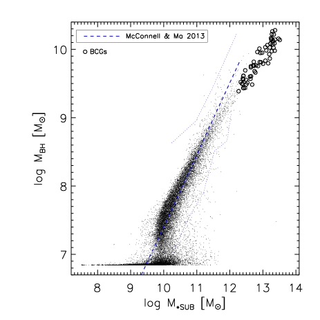
Figure 1: Correlation between the subhalo stellar mass and SMBH mass in our simulations. All subhaloes satisfying the BH seeding condition ($M>2.5\times 10^{11}h^{-1}$ M_⊙) have been included. The dashed line is a recent observational estimate of the $M_{BH}-M_{bulge}$ relation for a sample of 35 galaxies, of mixed morphological type, plotted only in the range covered by data (McConnell & Ma 2013). The two dotted curves enclose the region containing the data. Open circles refer to BCGs, for which a substantial contribution to $M_{*SUB}$ arises from intra cluster light. The concentration of points at $\log M_{BH}\sim 6.8$ is due to the mass with which the BH are seeded in the subhaloes.

2.1.2 AGN feedback

Our model for the growth of Super-Massive Black Holes (SMBH) and related AGN feedback is derived from Springel et al. (2005), with some differences we introduced to adapt it to the lower resolution of cosmological simulations. In this section the model is quickly summarized, while more details, including justifications for the modifications, can be found in the Appendix.

• SMBH seeding and growth. The BHs are represented by means of collision-less particles, subject only to gravitational forces. When a DM halo is more massive than a given threshold $M_{th}$ and does not already contain a SMBH, a new one is seeded with an initial small mass of $M_{seed}=5\cdot 10^{6}h^{-1}$ M_⊙. We set $M_{th}=2.5\times 10^{11}h^{-1}$ M_⊙. The SMBH grows with an accretion rate given by the minimum between a Bondi accretion rate (Bondi, 1952), modified by the inclusion of a (large) multiplicative factor, and the Eddington limit. At variance with respect to the original model we do not subtract the corresponding mass from the surrounding gaseous component. This results in a small mass non-conservation, which can be neglected on galactic scales, while avoiding the gas depletion in the BH surroundings, on physical scales much larger (tens of kpc) than its physical sphere of influence. This unrealistic removal of gas has, among others, also the effect of artificially shallowing the gravitational potential in the innermost part of the haloes, making it easier for the BHs to drift away from it.

• SMBH advection and mergers. In order to avoid numerical artifacts, it is fundamental to keep the SMBH at the center of its DM halo, counteracting numerical effects that tend to move it away (Wurster & Thacker, 2013). To obtain this, we reposition at each time-step the SMBH particle at the position of the nearby particle, of whatever type, having the minimum value of the gravitational potential within the gravitational softening of the SMBH. When two BHs are within the gravitational softening and their relative velocity is smaller than a fraction 0.5 of the sound velocity of the surrounding gas, we merge them.

• Thermal Energy distribution. In our model, the SMBH growth produces an energy determined by a parameter $\epsilon_{r}$ which gives the fraction of accreted mass which is converted in energy. Another parameter $\epsilon_{f}$ defines the fraction of this produced energy that is thermally coupled to the surrounding gas. These parameters are commonly calibrated in order to reproduce the observed scaling relations of SMBH mass in spheroids (see Section 3). Here we set $\epsilon_{r}=0.2$ and $\epsilon_{f}=0.2$, which results in a reasonable match with a recent estimate of the correlation between stellar and BH mass in spheroids (McConnell & Ma 2013), as shown in Fig. 1. We explicitly note that these values are greater than those adopted by other authors. However, we found that decreasing either $\epsilon_{r}$ or $\epsilon_{f}$ by a factor $\sim 2$, would increase the BH mass by a factor $\sim 2$ for a given stellar mass, significantly worsening the match shown in Fig. 1. Note that the simulation points at $\log M_{BH}\,\lower 2.0pt\hbox{${>\atop\hbox{\raise 4.0pt\hbox{$\sim$}}}$}\,9.2$ in this figure mostly refer to BCGs (open circles), for which a substantial contribution $\sim 50\%$ to $M_{*SUB}$ arises from Intra Cluster Light (ICL; e.g. Cui et al. 2013). A proper estimate of the BCG stellar mass (the subject of next Section 2.2) yields to a better agreement with the data at the high mass end (see Fig. 4).

  Following Sijacky et al. (2007), we also assume a transition from a quasar mode to a radio mode AGN feedback when the accretion rate becomes smaller than a given limit, $\dot{M}_{BH}/\dot{M}_{Edd}=10^{-2}$. In this case, we increase the feedback efficiency $\epsilon_{f}$ by a factor four.

  In the original model of Springel et al. (2005), the resulting energy was simply added to the specific internal energy of gas particles. However, due to the features of the adopted star formation and stellar feedback multi-phase model (Springel & Hernquist, 2003), when this energy is given to a star forming particle, it is almost completely lost without practical effects on the system (see Appendix A.4). To avoid this, whenever a star-forming gas particle receives energy from a SMBH, we calculate the temperature at which the cold gas phase would be heated by it. If this temperature turns out to be larger than the average temperature of the gas particle (before receiving AGN energy), we consider the particle not to be multi-phase anymore and prevent it from forming stars. To avoid an immediate re-entering of this gas particle in multi-phase star forming state, we add to the usual minimum density condition, a maximum temperature condition for a particle to be star forming, as anticipated in Section 2.1.1.

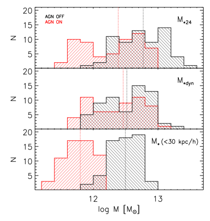
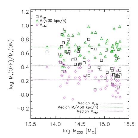
Figure 2: Left panel: histograms of the stellar masses of the BCGs, according to three different definitions (see text) for runs with AGN ON and OFF. The vertical lines show the median of the distributions. Right panel: ratios between the masses of the simulated BCGs without and with AGN feedback included, as a function of halo mass, for the same three definitions of BCG mass. The horizontal lines mark the median, with the same colours as the points for the three definitions.

2.2 Surface brightness maps

To generate mock maps of the clusters, we follow the same procedure as in Cui et al. (2013) and Cui et al. (2011). Each star particle is treated as a Simple Stellar Population (SSP) with age, metallicity and mass given by the corresponding particle properties in the simulation, and adopting the same initial mass function (IMF) (a Chabrier IMF; Chabrier 2003). The spectral energy distribution (SED) of this particle is computed by interpolating the SSP templates of Bruzual & Charlot (2003), and a standard Johnson V-band filter is applied to this SED, to get its V-band luminosity. Then, we smooth to a 3D mesh grid both the luminosity and the mass of each star particle with a SPH kernel. The mesh size is fixed to $5~{}h^{-1}~{}{\rm kpc}$ (corresponding to the simulation’s softening length). Finally, by projecting this 3D mesh in one direction we obtain the mock 2D photometric image. The procedure neglects dust reprocessing.

The simulated maps of the clusters have been used to compute isophotal radii, masses within these radii and half light (effective) radii of BCGs. In particular, we are interested in defining the total extent and mass of galaxies from mock maps, emulating what would be done using real observations. This is notoriously a difficult, if not an ill-posed, problem. Here, we generally follow a commonly adopted definition of the outer limit of galaxies, namely the isophote 25 mag arcsec^-2 in the B band, which for BCGs translates to about 24 mag arcsec^-2 in the V band. This isophotal boundary is at the basis of the D25 diameter and corresponding R25 radius, widely used in literature since its introduction by de Vaucouleurs et al. (1976). However, it is well known that this limit tends to underestimate the real extension of galaxies, so that we have also checked that our conclusions are substantially unchanged, and if anything strengthened, by adopting flux limits $\sim 1$ mag fainter.

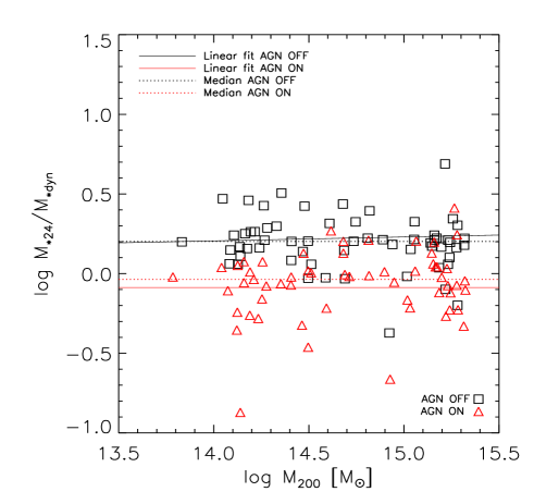
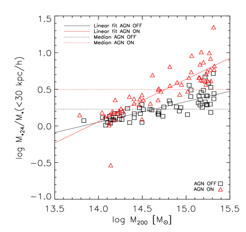
Figure 3: Left panel: Ratios between the BCG mass enclosed within the 24 mag arcsec^-2 in the V band, and that obtained by means of a dynamical separation from ICL (Cui et al. 2013; see text for more details) as a function of the halo mass. Right panel: the same but with the former mass replaced by the stellar mass within a radius of 30 kpc/$h$.

3 Results

3.1 The effect of AGN feedback on BCG mass

For almost a decade, AGN feedback has begun to be taken into account in galaxy formation, in order to avoid the prediction of too massive and too young galaxies. Actually, its relevance is quite plausible from a physical point of view. For instance, it is easy to see that, given the observed ratio of SMBH to stellar mass in spheroids, it is sufficient a very small fraction (a few percent), of the energy produced by accretion onto the SMBH to totally unbind the gas from the potential well of the galaxy. On the other hand, it has been well assessed that computations without some efficient inhibition of stellar mass assembly at the high mass end of the luminosity function, where SNae feedback becomes increasingly insufficient, over-predict the stellar mass by a factor $\,\lower 2.0pt\hbox{${>\atop\hbox{\raise 4.0pt\hbox{$\sim$}}}$}\,10$ (e.g. Benson et al. 2003). Negative feedback coming from AGN activity helps in reducing, if not totally solving, this problem.

In the left panel of Fig. 2 we show the distributions of the stellar masses of the BCGs, for runs with AGN ON and OFF, while the right panel displays the ratio between the masses of the same BCGs in AGN OFF and AGN ON simulation, as a function of hosting halo mass. Here we adopt three different possible definitions of the stellar mass. $M_{*24}$ is the mass enclosed by the 24 V mag/arcsec² isophote, mimicking a commonly adopted procedure to estimate total galaxy masses from observed images, as discussed in Section 2.2. $M_{*dyn}$ is instead the BCG mass computed performing a dynamical separation from the ICL, or more precisely from star particles not gravitationally bound to the galaxy, by means of an analysis of the velocity distribution. In brief, the method consists in recognizing that the latter is best fitted by the superposition of two Maxwellians, and in ascribing the low and high velocity components to the BCG and ICL respectively. Individual stellar particles are then assigned to the two components by means of an analysis of their velocities (see Cui et al. 2013 for details and references). Finally, $M_{*}(<30\ \mbox{kpc}/h)$ is the mass enclosed within a fixed radius from the galaxy center (defined as the center of mass of the stellar component). This simple choice of estimating the mass within a fixed physical radius has often been adopted to extract BCGs in hydro simulations. For instance McCarthy et al. (2010) and Stott et al. (2012) adopted 30 kpc$/h$, while Sijacki et al. (2007) used 20 kpc/$h$. However, this criterion is not well justified from an observational point of view (see below).

The two panels of Fig. 2 show that the inclusion of the AGN feedback indeed decreases the stellar mass. However the average decrease is only by a modest factor $\sim$ 1.5-5, depending on the adopted definition of mass. As we will see in more detail below, this is helpful but still un-sufficient for a satisfactory comparison with real galaxies. For $M_{*24}$, i.e. the mass obtained by means of a procedure close to an observational one, (and to a lesser extent also for $M_{*dyn}$) the decrease tends to be less pronounced in more massive haloes.

Fig. 3, left panel (see also left panel of Fig. 2), illustrates that $M_{*24}$ is on average $\sim 60$% larger than $M_{*dyn}$ for AGN OFF simulations, but only $\sim 15$% smaller for AGN ON runs, and that the ratios between these two masses do not have a clear trend with the halo mass. Indeed, Cui et al. (2013), analyzing this same set of simulations, find that the brightness profile of stars not dynamically bound to the BCG (i.e. not entering in the computations of $M_{*dyn}$), begins to dominate over that of the bound component on average at $\mu_{V}\,\lower 2.0pt\hbox{${>\atop\hbox{\raise 4.0pt\hbox{$\sim$}}}$}\,23$ mag/arcsec² for AGN OFF runs, with a weak dependence on mass. This limit turns out to be brighter enough than our adopted isophotal boundary ($\mu_{V}\,\lower 2.0pt\hbox{${>\atop\hbox{\raise 4.0pt\hbox{$\sim$}}}$}\,24$ mag/arcsec²) to exclude a fraction $\sim 50\%$ of the mass included by the latter. Conversely, the transition occurs at ($\mu_{V}\,\lower 2.0pt\hbox{${>\atop\hbox{\raise 4.0pt\hbox{$\sim$}}}$}\,24.75$) for AGN ON runs, almost independent of mass, a value fainter than our limit, which however does not add much mass.

Also the ratios between $M_{*24}$ and $M_{*}(<30\ \mbox{kpc}/h)$ depend on the flavor of the simulation, being on average over the whole sample $\sim 1.7$ and $\sim 3$ for AGN OFF and for AGN ON respectively (see right panel of Fig. 3 and also left panel of Fig. 2). However these ratios feature a quite evident trend with the halo mass, ranging from slightly more than 1, up to 2 and 5 respectively. Therefore, $M_{*}(<30\ \mbox{kpc})$ in general underestimates the BCG stellar mass, both with respect to the surface brightness limit and to the dynamical criterion. The problem worsen for AGN ON runs, since AGN feedback, besides making galaxies less massive, expands them (see Fig. 7 and related discussion below). Thus the use of a fixed physical radius to estimate stellar quantities introduces a bias, depending on the mass and on the sub-grid physics included. In particular, for the scope of the present paper, it can overstate the effectiveness of the AGN feedback in limiting the mass growth of galaxies, especially at high masses. We will come back to this point in Section 3.4.

For the above reasons, when comparing our results with data on total masses of BCGs, we adopt in the following $M_{*24}$, which is obtained mimicking a procedure often adopted in analyzing observations. However, it is reassuring to note that our conclusions would not be substantially affected by the use of $M_{*dyn}$.

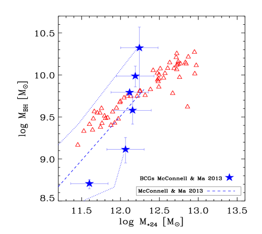
Figure 4: Correlation between the stellar and SMBH masses compared to a recent observational determination by McConnnell and Ma (2013), for a mixed sample of 35 galaxies with dynamically estimated bulge masses, and including 6 BCGs at the high mass end, plotted only in the range covered by data. The two dotted curves enclose the region containing all the available data, of which we plot only BCGs (blue stars).

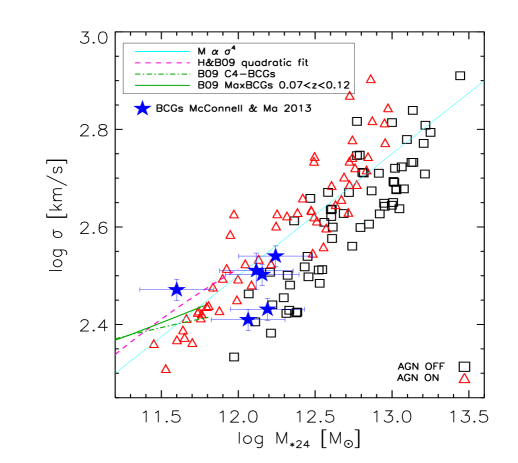
Figure 5: Correlation between the stellar mass and central (within $R_{e}/8$) 1-d velocity dispersion for our mock BCGs (Faber-Jackson relation), compared to recent estimates by Hyde & Bernardi (2009; H&B09) for elliptical galaxies and by Bernardi (2009; B09) for BCGs. These are plotted only in the range covered by their BCGs. The runs with and without AGN feedback are in red and black respectively.

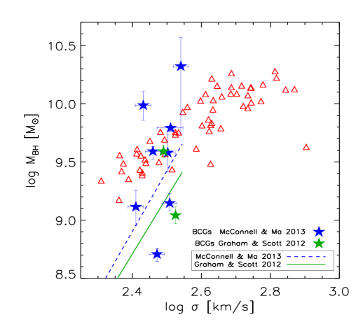
Figure 6: Correlation between the SMBH masses and stellar central (within $R_{e}/8$) 1-d velocity dispersion for our mock BCGs, compared to the determination by McConell & Ma (2013) for 53 Early Type Galaxies, including 8 BCGs, and that by Graham & Scott (2013) for 28 Ellipticals, two of which are BCGs.

3.2 SMBH mass vs BCG mass and velocity dispersion

When implementing in simulations sub resolution prescriptions for the growth of SMBH and for the ensuing feedback, the first basic requirement is to reproduce the observed correlation between the SMBH mass and the velocity dispersion, or the stellar mass, found for the spheroidal component of galaxies. Actually, the parameters entering in the sub-grid prescription for SMBH growth and AGN feedback, namely the accretion efficiency, the coefficient $\alpha$ in front of the Bondi accretion rate and the fraction of accretion energy thermally released to the interstellar medium (Eqs. 2, 3 and 4), have been calibrated here, as well as in previous works, in order to reproduce the $M_{BH}-M_{*}$ relationship, over the whole mass range accessible with the simulation (see Figure 1 and Section 2.1).

In view of this, Fig. 4 unsurprisingly shows that, once the stellar mass of the BCGs has been properly computed, correcting $M_{*SUB}$ for the ICL contamination, their relationship between the stellar and SMBH mass turns out to be in better agreement with that derived from observations, although with a somewhat shallower slope ($M_{BH}\propto M_{*}^{\alpha}$ with $\alpha\sim 0.7$ while $\alpha\sim 1$ in observation). Here we compare in particular our simulated BCGs with the recent observational determination by McConnnell & Ma (2013), for a mixed sample of 35 galaxies with dynamically estimated bulge masses, and including 6 BCGs, at the high mass end. Unfortunately, these BCGs have all (but one) similar masses within a factor $\,\lower 2.0pt\hbox{${<\atop\hbox{\raise 4.0pt\hbox{$\sim$}}}$}\,2$. As a consequence, while there is mounting evidence that these special objects differ from the general early type galaxy population for some other scaling relations (e.g. Hyde & Bernardi 2009; Berardi 2009), no conclusion can be drawn for the $M_{BH}-M_{*}$ relation. The simulated points extend to masses larger than observed by a factor $\sim 4$. This is a first general indication of the fact that even in our AGN ON runs the formation of baryonic structures is not prevented enough. This point will be addressed in Section 3.4. Note that, although we find in simulations a shallower slope than that found considering the whole early type galaxy population, the few observed BCGs scatter quite evenly around the region defined by the simulated points. Also, the intrinsic dispersion of real galaxies around the relationship is larger than that of simulated galaxies, as can be appreciated also from Figure 1. This can be due to an underestimate of the observational uncertainties, or to a physical link between star formation and SMBH accretion somewhat looser than that assumed in our simulation.

Since the ’70s, it has been known that the luminosity, or stellar mass, of early type galaxies strongly correlates with their velocity dispersion, $M_{*}\propto\sigma^{\gamma}$ with $\gamma\simeq 4$ (Faber & Jackson, 1976). More recently, it has been pointed out that this relationship shows a curvature at the high mass end, and in particular for BCGs, in the sense that the increase of $\sigma$ with stellar mass becomes slower, with $\gamma\simeq 5-6$ (Hyde & Bernardi 2009; Bernardi 2009). Fig. 5 shows the simulated Faber-Jackson relationship for AGN ON and AGN OFF runs, where $\sigma$ is the one dimensional velocity dispersion computed within $R_{e}/8$. The slopes are similar but in the former case the normalization is closer to observations. In both cases we get an increase of velocity dispersion with stellar mass described by $\gamma\sim 3$, faster than that of the general population of early type galaxies. This disagreement becomes more important if we consider the study by Bernardi (2009), based on two samples of thousands of BCGs. Moreover, there are no known BCGs with $\sigma>400$ km/s (e.g. von der Linden et al. 2007), while several simulated BCGs have $\sigma$ well above this limit. An important point to notice is that our AGN feedback, while decreasing the final stellar mass by a factor of a few, affects very little the predicted stellar velocity dispersion. In other words, the inclusion of AGN feedback moves the points in Fig. 5 almost horizontally to the left. Thus, while one could possibly imagine to reduce the residual over prediction of stellar masses with an even more aggressive choice of parameters, it is unlikely that this would help in making the velocity dispersions closer to the observed values. We will come back to this issue in Section 4.

The correlation between the SMBH mass and the central velocity dispersion $\sigma$ is shown in Fig. 6, and compared to recent observational determinations. McConnell & Ma (2013) provide the fit for a sample of 53 early type galaxies, including 8 BCGs, while Graham & Scott (2013) give a bisector regression for a sample of 28 ellipticals, two of which are BCGs. In both cases, the BCGs occupy a narrow $\sigma$ range, at the high end. These recent observational estimates point to a scaling of SMBH mass with $\sigma$ as steep as $M_{BH}\propto\sigma^{5}$, while our simulated BCGs are clearly characterized by a much shallower power law slope $\sim 2$. This is in keeping with the findings, presented in Fig. 4 and Fig. 5, that in our BCGs $M_{*}\propto\sigma^{3}$ and $M_{BH}\propto M_{*}^{0.7}$. As a result, while in the range of $\sigma$ covered by observations the simulated SMBH masses are larger than observed, if the observed correlation is extrapolated to larger masses, the opposite becomes true. Although the simulated point follow a quite shallower $M_{BH}-\sigma$ relationship than that defined by the whole early type galaxy population, the few observed BCGs are distributed around the former with a larger dispersion, similarly to the case of the $M_{BH}-M_{*}$

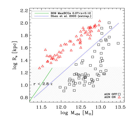
Figure 7: Effective radius against total stellar mass, computed within 24 magnitude in the V band, compared to the observed correlation in BCG (Bernardi 2009; plotted only in the region constrained by data), and to the extrapolation of the correlation derived for the global early type galaxies population by Shen et al. (2003). The runs with and without AGN feedback are in red and black respectively. The hatched area highlights the scale $2.8\epsilon$ over which, due to softening, the gravitational force deviates from the pure Newton law, although in most papers $\epsilon$ is regarded as the spatial resolution limit.

3.3 Mass-size relation

Normal Early Type Galaxies (ETGs) obey a well defined relationship between their stellar mass and effective radius $R\propto M^{0.6}$ (Mass-Radius Relation or MRR), as pointed out already by Burstein et al. (1997), and later substantially confirmed by various authors on the basis of the Sloan Digital Sky Survey (SDSS). As for BCGs, there have been both claims for a steeper slope $R\propto M^{0.9}$ (e.g. Bernardi 2009, Guo et al. 2009), as well as for no substantial deviation with respect to normal ETGs (von der Linden et al. 2007). In Fig. 7 we plot the effective radius against total stellar mass. The latter has been computed within the 24 mag/arcsec² V band isophote, for our mock BCG images, following a common observational definition (Section 2.2). In the same vein, the effective radius has been evaluated as the mean radius of the isophote enclosing half of the total light within the 24 mag/arcsec² V. The blue dotted line line is an extrapolation (at masses $>10^{12}M_{\odot}$) of the MRR relationship for ETGs by Shen et al. 2003, the short green line on the left is the fit given by Bernardi (2009) for BCGs in the redshifts bin $0.07<z<0.12$. The latter is plotted only in the range of masses in which it is actually derived, meaning that there are no BCGs in her sample whose stellar mass is larger than $10^{12}$ M_⊙. The figure shows that SMBHs feedback, besides making the galaxies less massive, with a greater effect at low masses, induces also a significative expansion by an average factor $\sim 4$. As a result, while the AGN OFF points lies below the extrapolations of both observed MRRs, the AGN ON are mostly above the Shen et al. (2003) MRR. By converse, the steeper law found by Bernardi (2009) for BCGs, when extrapolated to our mass range, would predict even larger galaxies. It is also interesting to note that the dispersion of the simulated correlation is much smaller in the AGN ON case. This supports, from a different point of view, the suggestion made by Ragone-Figueroa & Granato (2011). Using controlled numerical experiments, they proposed that AGN driven winds could have a role in explaining the low scatter of the observed local mass-size relationship (Shen et al. 2003; Bernardi 2009). This contribution may arise from the trade-off they found between variations of the assumed pre-wind galaxy size, and the amplification due to the wind driven mass loss. As a result, the post-wind size was found to be relatively insensitive to the initial one (see their figure 6).

Note that while AGN feedback clearly increases the effective radius, the same does not happen to the size of the 24 mag/arcsec² V band isophote, which we use to define the galaxy boundary. Indeed, we will see in Section 3.5 that the stellar density profiles are significantly flatter, with hints for a core, in the AGN ON runs. Our AGN feedback greatly affects the stellar density in the central regions, but little in the galaxy outskirts.

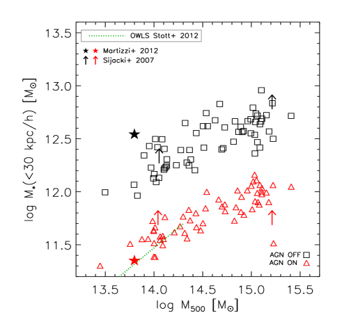
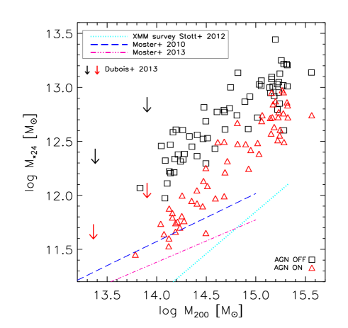
Figure 8: Left panel: stellar mass within 30 kpc/$h$ (as in Stott et al. 2012 for the OWLS simulation, green line) against $M_{500}$. Upward arrows mark the mass within 20 kpc/$h$ (hence lower limits in this plane, in particular for the high mass object) from the cosmological simulations of two galaxy clusters by Sijacki et al. 2007. Stars show the results by Martizzi et al. 2012a. They identified the BCG by means of a minimum stellar density criterium, but for their relatively small mass object the corresponding mass do not differ from $M_{*}(<30\ \mbox{kpc}/h)$ by more than 10%. Right panel: Stellar mass $M_{*24}$ enclosed by the 24 V mag/arcsec² isophote (a commonly adopted boundary for galaxies in observations) vs $M_{200}$, compared with recent abundance matching determinations (blue and purple lines) and with results from the XMM cluster survey (cyan line). All lines in these plot are plotted only in the region constrained by the data. The arrows show results of simulations by Dubois et al. 2013, for their two most massive galaxy groups. These are to be regarded as upper limits in this plot, since their estimate of the stellar mass of the central galaxy includes also the intra-cluster light. For all simulations, the runs with and without AGN feedback are plotted in red and black respectively.

3.4 The halo star formation efficiency

In Fig. 8, left panel, we compare our results on the relationship between the BCG stellar mass within 30 kpc/h and the halo mass $M_{500}$, with those by Stott et al. (2012) for the OWLS simulation. The latter simulations are also run with GADGET-3, but including a a different scheme for AGN feedback (Booth & Schaye 2009). In the mass range $3\times 10^{13}<M_{500}/\mbox{M}_{\odot}<2\times 10^{14}$, in which there is superposition between the two simulation sets, the agreement is good. In the higher mass regime covered by our simulations, there is a clear indication for a shallowing of the slope.

In the same plot, we have also reported the results obtained with the cosmological simulations of two galaxy clusters by Sijacki et al. 2007. We mark them as lower limits in this plane, since they estimated the BCG mass as the mass within 20 kpc/$h$. Finally, we include the results (stars) by Martizzi et al. 2012a, who identified the BCG by means of a minimum stellar density criterium. They claim that the corresponding mass does not differ from $M_{*}(<30\ \mbox{kpc}/h)$ by more than 10%.

We have already remarked (see discussion of Fig. 3) that the stellar mass computed within 30 kpc/$h$ is in general an underestimate of simulated BCGs total stellar mass, and that this underestimate is more severe for more massive galaxies, and when AGN feedback is included. As a consequence, its use provides an optimistic measure of the effectiveness of this physical process in limiting the stellar mass. As for observations, it is worth mentioning that Stott et al. (2011) found, for a local sample of BGCs, a mean value of the effective radius of $43.2$ kpc. Moreover, for a typical early type galaxy profile, the half mass radius is even larger than the half light radius. Thus the stellar mass within 30/$h\sim 40$ kpc in real BCGs is on average significantly less than half of the total mass. In conclusion, the practise of computing BCG stellar masses from simulations within $\sim 30-40$ kpc, in order to compare with total BCGs masses derived from observations is misleading.

For these reasons, in the right panel of Fig. 8 we compare with observations $M_{*24}$ against $M_{200}$. The arrows show results of simulations by Dubois et al. 2013, for their two most massive galaxy groups. They are reported as upper limits, since their estimate of the stellar mass of the central galaxy includes also the intra-cluster light. The cyan dotted line is a fit to observational estimates of the total stellar mass (from profile fitting) for the XMM cluster survey, given by Stott et al. (2012). We also plot recent determinations of this relationship based on the abundance matching technique (Moster et al. 2010, 2013). These are characterized by a slope, in the relevant mass range, much shallower than that found by Stott et al. (2012), and more in keeping with some other observational determinations (e.g. Lin & Mohr 2004; Popesso et al. 2007; Guo et al. 2009). If this slope is confirmed, the figure shows that our simulations, even with AGN feedback included, increasingly over-predict the BCG stellar mass with increasing halo mass. The use of $M(<30\ \mbox{kpc}/h)$ to estimate the BCG mass would largely mask the problem. In the low mass region, AGN ON simulations produce an amount of stars in relative agreement with observational estimates.

Our finding that AGN feedback helps to decrease the masses of BCGs, but falls short of reducing them to the observed values in massive clusters, is in good agreement also with the results shown by Puchwein et al. 2010 for BCGs luminosities (see their figure 8), and by Puchwein & Springel 2010 (their figure 5). To exacerbate the problem, we note that the over-prediction of stellar mass in our, and most other simulations, could be in part artificially reduced by the use of SPH technique to treat hydrodynamics. Indeed, it has been claimed that this method suffers a form of numerical quenching of cooling, particularly important in large haloes. Indeed, Vogelsberger et al. (2013) found that, using the novel moving mesh method for the hydrodynamical forces, it is necessary to invoke very strong forms of stellar and AGN feedback in order to reasonably reproduce the local galaxy luminosity function in cosmological simulations. More specifically, they had to increase significantly the strength of radio-mode feedback, compared to previous studies, and to adopt an energy per SNII event three times larger than the canonical one. Still, the bright end of the luminosity function remains somewhat overproduced.

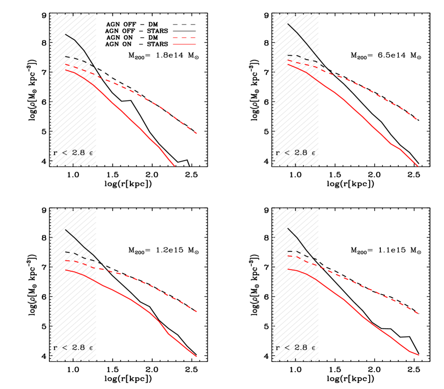
Figure 9: Density profiles for 4 representative clusters. Is is apparent that AGN feedback produces a significant flattening of the inner stellar and, to a lesser extent, DM profiles. The hatched areas highlight the scale $2.8\epsilon$ over which, due to softening, the gravitational force deviates from the pure Newton law. Note that in most papers $\epsilon$ (where the plotted lines begin) is regarded as the spatial resolution limit.

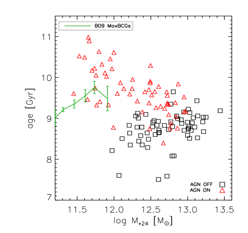
Figure 10: Mass averaged ages, within 24 mag arcsec^-2 in the V band, of stellar particles as a function of total stellar mass in simulated BCGs, compared with observational estimates by Bernardi (2009).

3.5 The effect of AGN feedback on density profiles

A few papers have pointed out recently that AGN feedback can flatten the central ($\sim 10$ kpc) density profiles of both stars and DM in massive galaxies. As for stellar profiles, this has been shown to be the case either using idealized numerical experiments (Ragone-Figueroa & Granato 2011; Martizzi et al. 2013) or cosmological zoom-in high resolution simulation of a few clusters (Sijacki et al. 2007; Puchwein et al. 2010; Martizzi et al. 2012a,b). As for the DM component, it has been shown that the expansion driven on its density profile by the strong AGN feedback, required to match the low star formation efficiencies of large DM halos inferred from observations (e.g. Moster et al. 2013), more than counteracts the opposite contraction caused by baryon condensation, both in cosmological as well as in controlled simulations (Duffy et al. 2010; Ragone-Figueroa, Granato & Abadi 2012). As a matter of fact, cuspy density profiles of DM in large ETGs, tentatively inferred from some recent observation (e.g. Tortora et al. 2010), could be difficult to reconcile with an strong AGN feedback.

Our intermediate resolution simulations of a relatively large sample of clusters confirm this finding. In Fig. 9 we show the density profiles for the BCGs of 4 representative clusters. Comparing the predicted profiles with and without AGN feedback, it is apparent that this process has the average effect of flattening the inner ($R\,\lower 2.0pt\hbox{${<\atop\hbox{\raise 4.0pt\hbox{$\sim$}}}$}\,30$ kpc) stellar profiles. The flattening becomes more and more pronounced going toward the center, hinting to a core starting at $\sim 10-15$ kpc. Although this scale is only 2-3 times the gravitational softening, and thus about our resolution limit, Martizzi et al. (2012a), with a spatial resolution five times better, found a core of the same size, which may suggest that we are witnessing to a real effect, rather than just a numerical artifact. Even the DM profile is flattened by the inclusion of AGN feedback by a sizeable amount.

It is worth noticing that the prediction of cored inner profiles of stars, over scales of $\sim 10$ kpc, has been regarded as a success of the simulations including AGN feedback (Martizzi et al. 2012a,b), because there have been reports of cores in observed profiles of cluster elliptical galaxies. However, the sizes of observed cores are at least one order of magnitude smaller, say $\,\lower 2.0pt\hbox{${<\atop\hbox{\raise 4.0pt\hbox{$\sim$}}}$}\,1$ kpc (see for instance figure 39 in Kormendy et al. 2009). Therefore, a final assessment on the capability of simulations to reproduce the correct inner density profiles of BCGs would require much higher resolutions than that of the simulations presented here. Nevertheless, it seems already established the fact that current models of AGN feedback produce stellar cores, or significative flattening of stellar profiles, on relatively well resolved scales, and much larger than observed. Thus, on one hand present day sub-resolution models of AGN feedback are not effective enough in diminishing the global formation of stars in the most massive galaxies, but on the other hand they seem to be relatively too effective in their centers.

Also, with AGN included, the baryonic component becomes subdominant down to the most internal regions accessible at our resolution limit. Actually, several studies point to an important, or even dominant, contribution to the gravitational field from DM within $R_{e}$ in bright ETGs (e.g. Tortora et al. 2012; McConnell et al. 2012; Grillo 2010).

3.6 Stellar ages

In Fig. 10 we show the mass averaged ages of stellar particles as a function of total stellar mass in simulated BCGs. These are compared with the observational estimates given by Bernardi (2009). It is apparent that the inclusion of AGN feedback, besides reducing the total mass, thus shifting the points leftwards, increases the average age by 0.5-2 Gyr, moving the points upwards. However, the effect decreases with increasing mass, resulting in a slight decrease of the age going to higher masses, a trend not confirmed by observations. This seems to be another manifestation, together with the excessive stellar masses, of the progressively insufficient quenching effect of AGN feedback prescription in massive galaxies.

Consistently with the less prolonged star forming phase in AGN ON simulations, the corresponding BCG mass averaged stellar metallicity turns out to be slightly lower. The predicted metallicity is essentially independent of the galaxy mass, and is on average about 0.8 and 0.6 solar in AGN OFF and AGN ON runs respectively.

4 Discussion and conclusions

AGN feedback is widely recognized as a required ingredient for simulations, to avoid the formation of excessively massive galaxies. Indeed, the approximate inclusion of this effect into our simulated clusters, alleviates the tensions with observational constraints on the baryonic budget in the various components of clusters and groups (this work; Planelles et al. 2013). In particular, we have analyzed here the basic properties of BCGs, finding that AGN ON simulations go in the right direction of reducing by a factor of a few the final stellar mass of these exceptional objects.

Nevertheless, the results obtained with our implementation of AGN feedback (similar to that of most cosmological simulations) are only partially satisfactory. The stellar mass remains still too large by a significant factor, greater than two and increasing with halo mass, with respect to real BCGs, a problem which is shared by other numerical works (Fig. 8). Also, their basic structural features show some disagreement with observations. Indeed, the predicted half light radius at a given stellar mass is larger than observed (Fig. 7). The AGN feedback causes a significant flattening of the stellar density profiles. This flattening increases with decreasing radius, and suggests almost cored profiles extending to much larger radii than observed (Fig. 9). It is unlikely that the latter feature is only due to effects of spatial resolution, since cores of similar sizes ($\sim 10$ kpc) have been observed in other higher resolution simulations, including AGN feedback (Martizzi et al. 2012a).

We found that our AGN feedback, while decreasing the final stellar mass by a factor of a few, affects very little the predicted stellar velocity dispersion (the inclusion of AGN feedback shifts the points in Fig. 5 almost horizontally to the left). It appears therefore unlikely that a more aggressive choice of parameters, which could reduce the still excessive stellar mass, would also reduce the velocity dispersions, to better match the observed values. In order to achieve this, a more fundamental change in the AGN feedback model seems to be required. A significative decrease of $\sigma$ can be attained by large scale outflows of gas, as shown by the controlled numerical experiments by Ragone-Figueroa & Granato (2011). They followed the dynamical evolution of a spheroidal stellar system, embedded in a dark matter halo, after the rapid ejection of large amount of gas. For instance, they found that if the expelled gas mass is $\sim 40\%$ of the initial baryon content of the galaxy, the velocity dispersion of stars can be reduced by $\sim 30\%$ (their figure 4). Moreover, Dubois et al. (2013) run cosmological zoom-in simulations for the formation of six early type galaxies, in which the AGN feedback has been included in a kinetic rather than thermal form. In principle, the substantial decrease of velocity dispersion they found, with respect to the no AGN case (see their figure 18), can arise from two causes: the shallowing of potential well due to the gas expulsion, and the quenching of the in situ star formation, which transforms these galaxies into systems built up mostly by accretion and minor mergers. Indeed, in minor mergers the velocity dispersion can decrease inversely proportional to the mass, as can be shown by means of simple virial theorem arguments (e.g. Bezanson et al. 2009; Naab et al. 2009). However, Ragone-Figueroa & Granato (2011) demonstrated that the former cause alone can have an important effect in decreasing the velocity dispersion. Moreover the “in situ quenching” is, at least in part, present also in simulations with thermal AGN feedback, which however does not produce by itself important gas outflows (Barai et al.  2013). In conclusion, outflows appear to be the best candidates for obtaining values of stellar velocity dispersions closer to observed ones.

Among the various relationships we considered, when comparing AGN ON with AGN OFF runs, we found that the former are characterized by a similar or lower spread. This is particularly evident for the mass-size relations (Fig. 7), and we have proposed a possible physical explanation, based on results of our previous work (Ragone-Figueroa & Granato, 2011). Conversely, McCarthy et al. 2010 found a clearly greater spread in the (different) relationships they considered, when AGN feedback was included in the OWLS simulation. They do not attempt an explanation for that, and it is impossible for us to assess the origin of their different result. However, we notice that when we did test runs adopting different, less effective, advection prescriptions to keep the SMBH at the centers of galaxies (see Appendix A.3), our decrease of the dispersion in the relationships obtained from AGN ON runs was largely masked or reversed.

It may be noticed that the dispersions of the $M_{BH}-M_{*}$ and $M_{BH}-M_{\sigma}$ relations produced by the simulations seem significantly smaller than observed, taking into account the declared observational uncertainties (Figs. 1, 4, 6). Unless the latter are underestimated, this suggests a link between the growth of stellar mass and that of the SMBH less strict than that produced by the prescriptions we adopt. For instance, we do not take into account the evolution of BH spins (e.g. Barausse 2012), which would result in a distribution of radiative efficiencies rather than a single value, under the common assumption that they are set by the radius of the last stable orbit around the BH. The very small dispersions in simulations could also be contributed by a too effective BH merging, following galaxy merging. Indeed, it has been shown that merging of galaxies and their host BH tends to strengthen a preexisting correlation (Peng 2007).

In conclusion, the prescriptions adopted so far in our simulations to describe AGN feedback, similar if not identical to those of most cosmological simulations so far, while producing encouraging results especially for the global properties of clusters (e.g. Mccarthy et al. 2010; Fabjan et al. 2010; Planelles et al. 2013), seem to require substantial improvements. In particular, the effectiveness in diminishing the total star formation of most massive galaxies has to be increased, whilst the relative effectiveness in the central regions $r\,\lower 2.0pt\hbox{${<\atop\hbox{\raise 4.0pt\hbox{$\sim$}}}$}\,10$ kpc should be properly balanced downwards. In other words, the effect of AGN feedback should be more widely spread over the galaxy volume, likely by means of large scale gas outflows. These important outflows, that can be generated by kinetic AGN feedback, should also help in decreasing the predicted excessive velocity dispersion of BCGs, on which instead the adopted thermal feedback has little effect.

Appendix A AGN feedback model: tests

In this Appendix, we describe in more details the AGN feedback model, and we show some tests that justify our prescriptions as well as our parameters choice. To this aim, we use four different simulations of the same Lagrangian region, centered on a cluster having a mass $M_{200}=3.7\times 10^{14}$h^-1 M_⊙ at redshift $z=0$. This region is one among those we use in the main paper, and all simulation details, except for the AGN sector, are identical to those presented there. For the first simulation we used without modifications the original BH and AGN feedback model by Springel et al. (2005) (A-STD), but with our chosen values for the parameters describing radiative and feedback efficiencies, and a switch between quasar and radio modes (Sijacki et al. (2007); see Section A.1). The main problem in using plainly the original scheme A-STD, is that it was thought and calibrated for non-cosmological high resolution simulations of merging galaxies, and its use without some modifications leads, in the context of this paper, to several unwanted and misleading effects, described below. Leaving for future work the task of improving both the physical model, as well as that of making its implementation less resolution dependent, our approach here has been to introduce the minimal changes required to avoid unreasonable results.

In the other three simulations, we modify A-STD introducing one at a time the three distinctive features of our final model: (i) we do not allow the BHs to swallow gas from the simulation, as it would be predicted by their accretion rates (A-NOSW); (ii) we use our scheme for BHs advection and mergers (A-CNTR); and (iii) we use our prescription for the coupling of the AGN feedback energy to the gas particles (A-NWEN). Table 1 lists our test simulations.

Table 1: Test simulations for our AGN feedback modified model. Column 1: Simulation name; Column 2: Model used.

A-STD	Springel et al. (2005) model + quasar/radio mode
A-NOSW	As A-STD, but no gas removal from simulation
A-CNTR	As A-STD, but with our modification to the BH advection and merger schemes
A-NWEN	As A-STD, but with our new coupling between AGB feedback energy and gas particles

A.1 BH accretion and ensuing feedback

We identify DM haloes using an on-the-fly Friends-of-Friends algorithm. We seed a BH particle every time that a DM halo has a mass $M_{halo}>M_{th}=2.5\times 10^{11}h^{-1}$ and does not already contain a BH. We initially put the newly seeded BH at the position and with the velocity of the gas particle having the minimum gravitational potential energy, and we remove the latter from the simulation. The initial mass of the BH is set to $M_{seed}=5\times 10^{6}h^{-1}$ M_⊙, but see Section A.2.

As in most previous simulations with AGN feedback, also in our simulations the BH grows at a rate which is the minimum between what we dub $\alpha$-modified Bondi rate (Bondi, 1952) and the Eddington rate:

$$\dot{M}_{BH}=\min\left(\dot{M}_{Bondi,\alpha},\dot{M}_{Edd}\right)$$ (1)

The general idea is that the former should provide an order of magnitude estimate of the gas which potentially can feed the BH, given its physical conditions, without producing enough luminosity to reverse the flow, as controlled by the latter. Of course, we should remind that this is an over-simplification of a very complex process, and that these rates are obtained under several strong assumptions. As a result, they could even fail to provide a correct order of magnitude.

The $\alpha$-modified Bondi rate is

$$\dot{M}_{Bondi,\alpha}=\alpha\,4\pi\frac{G^{2}M^{2}_{BH}}{c^{2}_{s}+v^{2}_{BH}}\rho$$ (2)

where $M_{BH}$ is the BH mass, $v_{BH}$ its velocity (relative to the surrounding gas bulk motion), $c_{s}$ the sound velocity of the gas surrounding the BH and $\rho$ its density, and a fudge adimensional factor $\alpha\sim 100$ is included. This apparently arbitrary and large factor, has been initially justified simply by the pragmatic requirement of helping in producing a reasonable black hole mass at the end of the simulation. More recently, it has been perceived as a cure for the limitation of having to use gas properties numerically calculated on scales much larger than the BH sphere of influence. Indeed, we always estimate gas quantities using the SPH spline kernel, whose smoothing length is the radius of a sphere containing a mass of $4\times N_{neigh}M_{gas,init}$ ($N_{neigh}$ is the number of neighbours for hydro calculations and $M_{gas,init}$ the initial mass of gas particles). This scale length is typically $\,\lower 2.0pt\hbox{${>\atop\hbox{\raise 4.0pt\hbox{$\sim$}}}$}\,10$ kpc in cosmological simulation (see e.g. Fig. 11), thus is is much larger than the real scale over which the BH accretes its gas (as discussed at the end of Section A.2). The assumption that gas properties at scales as large as these are related to the corresponding small-scale is unjustified. Actually, Booth & Schaye (2009) pointed out that the un-sufficient resolutions underestimate the density and overestimate the sound speed by orders of magnitude, thus justifying large values of $\alpha$. However, this would suggest some relationship between $\alpha$ and the resolution.

The Eddington accretion rate is:

$$\dot{M}_{Edd}=4\pi\frac{c\,G\,m_{p}}{\epsilon_{r}c^{2}\sigma_{T}}M_{BH}$$ (3)

where $m_{p}$ is the proton mass, $\sigma_{T}$ the Thompson cross section, $c$ the speed of light and $\epsilon_{r}$ the radiative efficiency, giving the radiated energy in units of the energy associated to the accreted mass. Once we estimate the accretion rate, we assume that a fraction $\epsilon_{f}$ of the irradiated energy couples to the IGM/ICM gas and heats it. Thus the rate of available feedback energy from an AGN is:

$$\dot{E}_{feed}=\epsilon_{f}\epsilon_{r}\dot{M}_{BH}c^{2}$$ (4)

Finally, following Sijacki et al. (2007) we assume a transition from a quasar mode to a radio mode of AGN feedback. This occurs when the accretion rate becomes smaller than a given limit, $\dot{M}_{BH}/\dot{M}_{Edd}=10^{-2}$. In this case, we increase the feedback efficiency $\epsilon_{f}$ by a factor four.

We varied the parameters $\alpha$, $\epsilon_{r}$ and $\epsilon_{f}$ to match the BH mass- stellar mass relation (see Figs. 1 and 4). Our choice is $\alpha=100$, $\epsilon_{r}=0.2$ and $\epsilon_{f}=0.2$.

Figure 11: Histogram of the BH particles smoothing length in the test region, for the A-STD simulation at redshift 2. This is representative of the situation in the redshift range most relevant for BH activity.

A.2 Numerical aspects of BH gas accretion

The growth rate of SMBHs is calculated as described above. In literature, a scheme for removing gas from the simulation following as much as possible the BH mass accretion rate (”swallowing” of gas particle by BHs) is usually adopted, to ensure mass conservation. Commonly, gas particles within the smoothing length of BHs are randomly removed from the simulation, with a probability proportional to the SPH kernel, and their mass is added to the BH mass. Of course this leads to a very discretized representation of the process, and the problem is particularly severe in cosmological simulations, wherein the mass of a gas particles ($\sim 10^{8}M_{\odot}$ in our case) can be in the range of an already well developed SMBH. Also, the swallowing occurs often at distances orders of magnitude greater than the actual sphere of influence of the BH.

To cope with this, the models usually characterize the BH particles by means of two masses: a theoretical one $M_{BH,th}$, determined exactly by the BH accretion rate computed from the Eq. 1 and used for all the computations involving AGN feedback, and a dynamical BH mass $M_{BH,dyn}$, used for the gravitational and dynamical calculations. The latter is adjusted by swallowing gas particles from time to time, in order to keep it as close as possible to the theoretical mass. At seeding, the BH is created by converting a gas particle into a BH particle, with the same dynamical mass.

However, at the relatively low mass resolution of cosmological simulations like our own, the match between the two BH masses is quite unsatisfactory until the SMBH reaches a very high mass $\,\lower 2.0pt\hbox{${>\atop\hbox{\raise 4.0pt\hbox{$\sim$}}}$}\,10^{9}M_{\odot}$. For instance, at seeding, the BH begins its “life” with a dynamical mass orders of magnitude greater than the theoretical one. On the other hand, a later seeding, with a theoretical mass already close to the gas particle mass, would miss the feedback effects of the BH during an important part of its growth. In cosmological simulations, the large ratio $M_{BH,dyn}/M_{BH,th}$, which should approach unity while the BH grows by accretion, thanks to the algorithm of swallowing, can instead persist for BH particles of large theoretical masses, if their mass growth occurs mostly by mergers. This situation can occur particularly often when the numerical scheme leads to some overmerging (see Section A.3). In this case, the dynamical mass of the particle, used to compute its gravitational effects, can become really huge.

To avoid introducing artifacts due to the large difference between the two masses, we choose here to keep always the dynamical mass equal to the theoretical one, as given by the accretion formula Eq. 1. Given that this already means to give up to rigorous mass conservation, we also decided to avoid at all any swallowing of the gas particles. The resulting global error in term of mass non-conservation is small, of the order of a fraction of percent the stellar mass of the halo where the BH dwells, and can be neglected on galactic scales. The advantage is that it avoids the gas depletion on physical scales much larger than the real sphere of influence of SMBH.

Indeed, typical values of BH smoothing lengths are of the order of tens of kpc in the redshift range more relevant for BH accretion. An example for z=2 is shown in Fig. 11. By converse, the radius at which a central SMBH dominates the potential of the host galaxies is

$$r_{BH}\simeq 11\frac{M_{BH}}{10^{8}M_{\odot}}\left(\frac{\sigma}{200\,\mbox{km/s}}\right)^{-2}\mbox{pc}$$ (5)

or, assuming that the system obeys the observed correlation between stellar velocity dispersion $\sigma$ and BH mass,

$$r_{BH}\simeq 16\left(\frac{M_{BH}}{10^{8}M_{\odot}}\right)^{0.62}\mbox{pc}$$ (6)

where we have used the recent determination by McConnell & Ma (2013) for ETGs.

In particular, we found that this unrealistic removal of the gas has, among others, also the effect of un-physically shallowing the gravitational potential in the innermost part of the haloes, making it easier for the BHs to drift away from it.

A.3 BH advection and mergers

The effect of the feedback energy provided by SMBHs critically depends on the fact that particles representing them stay at the center of their parent DM haloes, where it is seeded (see e.g. Wurster & Thacker (2013)). In addition, if a BH un-physically exits from its parent DM halo, that halo becomes eligible for seeding another spurious BH. This stability is not attained by construction in large-scale numerical simulations, for two reasons. The first is that, when the BH has a dynamical mass still comparable to that of other numerical particles, it can be scattered around by two-body encounters. The second has to do with the chaotic nature of self-gravitating systems is. The trajectory of an individual numerical particle in phase-space is subject, due to numerical errors, to large deviations from the exact trajectory of a particle starting from the same initial conditions. This effect is particularly important for un-softened systems (see e.g. Quinlan & Tremaine 1992), but it cannot be ignored also when a softened gravitational force is used (see e.g. Hayes 2003). Therefore it is necessary to introduce an artificial advection algorithm to keep the SMBH as close as possible to the galactic center. In our case, at each time step of the BH particle, we force it at the position of the most bound particle, of whatever type, within the gravitational softening of the BH.

When two BHs are within the gravitational softening and their relative velocity is smaller than a fraction of the sound velocity of the surrounding gas, we merge them. We place the resulting BH at the position of the most massive one. This repositioning scheme clearly has the consequence of violating the momentum conservation; however, the aim of our numerical prescriptions is to reproduce some physical properties and effects emerging from unresolved scales, and not to directly simulate the BH physics. From this point of view, a limited non-conservation of momentum (or mass, Section A.2) is acceptable.

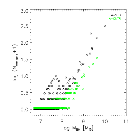
Figure 12: Total number of mergers of the BHs in the test region (down to z=0), against their mass, for the A-STD simulation, closely following the Springel et al. (2005) scheme, and the A-CTRL, in which instead our modifications for the advection and merging algorithms have been introduced.

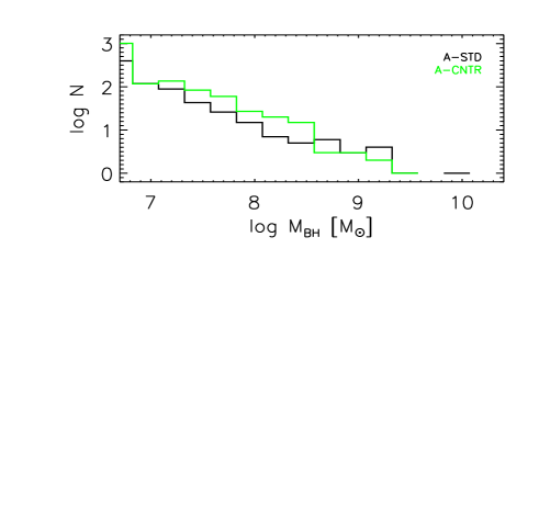
Figure 13: Mass distribution of BH at redshift $z=0$.

We explicitly note that we use the gravitational softening as a searching length, rather than the BH smoothing length as in most previous implementations, for both the advection and the merging algorithms. In principle, the former seems to be a more sensitive choice, because the numerical processes acting to drift away the BH, as well as the physical process leading to BH merging, are gravitational in nature. Furthermore, at the resolution of our simulations, the BH smoothing length is unreasonably large for these purposes, and significantly larger than the gravitational softening (Fig. 11). In particular, if we used the former for searching the minimum potential particle, BHs dwelling in satellite haloes could often be spuriously displaced to the center of a more massive DM halo, and immediately would merge with the BH dwelling there. This numerical over-merging affects the mass function of BH, artificially increasing by merging the final masses at the high mass end, and depleting the number of BH at low and intermediate masses. It is significantly reduced by repositioning within the softening length, as can be seen from Figures 12 and 13. For example, the most massive BH had 322 mergers in A-STD, which closely follows the Springel et al. (2005) scheme, but only 34 in A-CNTR, wherein our modifications for the advection and merging algorithms have been introduced. As a result, in the latter case its final mass is twice smaller.

A.4 Feedback energy distribution

In the original scheme by Springel et al. (2005), the AGN feedback energy is simply added to the specific internal energy of gas particles. Owing to the features of the effective model of star formation and stellar feedback (Springel & Hernquist, 2003), when SMBH energy is given to a star-forming gas particle, it is almost completely lost. This is due to the fact that any deviation of the internal energy from the equilibrium one rapidly decays, over a timescale shorter than a typical timestep.

Indeed, the total specific equilibrium energy is given by $u=(\rho_{h}u_{h}+\rho_{c}u_{c})\rho^{-1}$, where $u_{h}$ ($\rho_{h}$) and $u_{c}$ ($\rho_{c}$) are the equilibrium specific energies (densities) of the hot and cold phase respectively of the star-forming gas. $u_{c}$ is assumed to be constant, while

$$u_{h}=\frac{u_{SN}}{A+1}+u_{c}$$ (7)

where $A$ is the efficiency of evaporation of cold clouds in the Inter-Galactic Medium (IGM), taken to be $A\propto\rho^{-4/5}$; $u_{SN}$ is the specific energy provided by supernovae, also assumed constant (Springel & Hernquist, 2003).

From the same work, the time-scale over which deviations from this equilibrium energy decay is:

$$\tau_{h}=\frac{t_{*}\rho_{h}}{\beta(A+1)\rho_{c}}$$ (8)

where $t_{*}\propto\rho^{-1/2}$ is the star formation time-scale, $\rho$ being the average gas particle density; $\beta$ the mass fraction of stars which immediately explode as Type II supernovae. In particular, deviations due to an external source (external from the point of view of the effective model), such as AGN feedback evolves over a time-step $\Delta t$ to $u+(u^{out}-u)e^{-\Delta t/\tau_{h}}$, where $u^{out}$ is the energy provided from outside. In star-forming region, the higher the density of the gas is, the faster is the convergence to the equilibrium specific energy $u$ and the least effective is the AGN energy feedback. Any increase of internal specific energy of star-forming particles is immediately lost if the effective model for star formation and feedback is active.

To avoid this, whenever a star-forming gas particle receives energy from a SMBH, we now calculate the temperature $T_{c}$ at which the cold gas phase would be heated by it. The AGN energy is given to hot and cold phases proportionally to their mass, but since the mass fraction of the cold phase is high, this particular choice is not important. If $T_{c}$ turns out to be larger than the average temperature of the gas particle (before receiving AGN energy), we consider the particle not to be multi-phase anymore and prevent it from forming star. To avoid an immediate re-entering of this gas particle in the multi-phase star forming state, wherein it would immediately lose all of its internal specific energy in excess to the equilibrium one, we also add a maximum temperature condition to the usual minimum density condition for a gas particle to become multi-phase and form stars.

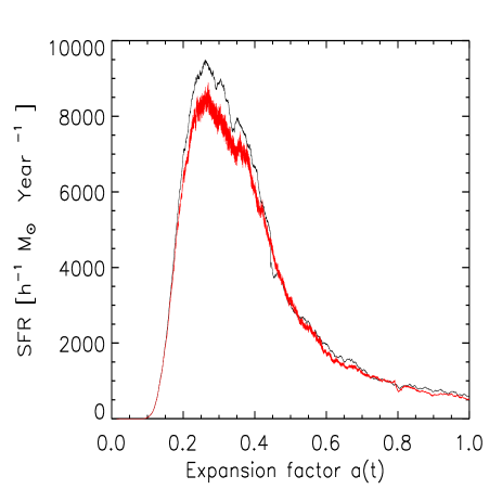
Figure 14: Star formation rate in our selected Lagrangian regions for simulation A-STD (black line) and A-NWEN (red line)

In Fig. 14, we show the effect of our new prescription on the overall star formation rate comparing simulation A-STD (black line) with A-NWEN (red line). A reduction of $\sim 10\%$ is appreciable at the peak of the star formation, which happens between redshift $z=3$ and $z=2.5$. The reason for this additional quenching can be understood from Fig. 15, where we show the density-temperature diagram of gas particles in simulations A-STD (black diamonds) and A-NWEN (red diamonds). We consider all the particles included in a sphere of radius $R=50$ h^-1 comoving kpc, centered on the most massive BH at redshift $z=2.8$. With the original prescription, even in presence of AGN feedback, gas particles remain very dense and star forming: the bulk of them stays on the effective equation of state given by the star formation model. This is tracked by the line shaped concentration of points in the lower right corner of the diagram. This is caused by the quick convergence to the equilibrium specific energy explained above. With our new scheme, gas is less dense, and more particles can reach temperatures higher than $10^{7}$K when receiving feedback energy, becoming non star forming. Thus, with our scheme the feedback energy acts in a more efficient way.

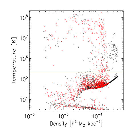
Figure 15: Phase diagram for gas particles in a sphere of radius $R=50$h^-1 comoving kpc, centered on the most massive BH at redshift $z=2.8$. Black diamonds: simulation A-STD; red diamonds: simulation A-NWEN. The horizontal line marks our adopted temperature threshold for a particle to become multi-phase and star-forming.

Finally, we also found that, contrarily to naive expectation, in the original model an increase of AGN feedback efficiency $\epsilon_{f}$ gives an increase in the star formation rate, rather than a reduction. This disturbing feature is due to the increase of gas pressure of star forming particles, caused by the action of non star-forming particles, heated by feedback, on the formers. Indeed, in the effective model of Springel & Hernquist (2003), an increase of gas pressure enhances the star formation. With our new scheme, this effect is reduced, since the pressure increase is partly balanced by a density decrease, as shown in Fig. 15. However it is still not eliminated. A substantial refinement of the AGN feedback prescriptions which pays particular attention to the interplay between AGN energy and star formation model is still needed in cosmological simulations.

References

- Barai et al. (2013) Barai P., Viel M., Murante G., Gaspari M., Borgani S., 2013, arXiv, arXiv:1307.5326
- Barausse (2012) Barausse E., 2012, MNRAS, 423, 2533
- Benson et al. (2003) Benson A. J., Bower R. G., Frenk C. S., Lacey C. G., Baugh C. M., Cole S., 2003, ApJ, 599, 38
- Benson (2010) Benson A. J., 2010, PhR, 495, 33
- Bernardi (2009) Bernardi M., 2009, MNRAS, 395, 1491
- Bezanson et al. (2009) Bezanson R., van Dokkum P. G., Tal T., Marchesini D., Kriek M., Franx M., Coppi P., 2009, ApJ, 697, 1290
- Bonafede et al. (2011) Bonafede A., Dolag K., Stasyszyn F., Murante G., Borgani S., 2011, MNRAS, 418, 2234
- Bondi (1952) Bondi, H, 1952, MNRAS, 112, 195
- Booth & Schaye (2009) Booth C. M., Schaye J., 2009, MNRAS, 398, 53
- Bower et al. (2006) Bower R. G., Benson A. J., Malbon R., Helly J. C., Frenk C. S., Baugh C. M., Cole S., Lacey C. G., 2006, MNRAS, 370, 645
- Burstein et al. (1997) Burstein D., Bender R., Faber S., Nolthenius R., 1997, AJ, 114, 1365
- Bruzual & Charlot (2003) Bruzual G., Charlot S., 2003, MNRAS, 344, 1000
- Chabrier (2003) Chabrier G., 2003, PASP, 115, 763
- Croton et al. (2006) Croton D. J., et al., 2006, MNRAS, 365, 11
- Cui et al. (2011) Cui W., Springel V., Yang X., De Lucia G., Borgani S., 2011, MNRAS, 416, 2997
- Cui et al. (2013) Cui W., et al. submitted
- de Vaucouleurs, de Vaucouleurs, & Corwin (1976) de Vaucouleurs G., de Vaucouleurs A., Corwin J. R., 1976, RC2, 0
- Dubois et al. (2013) Dubois Y., Gavazzi R., Peirani S., Silk J., 2013, MNRAS, 433, 3297
- Duffy et al. (2010) Duffy A. R., Schaye J., Kay S. T., Dalla Vecchia C., Battye R. A., Booth C. M., 2010, MNRAS, 405, 2161
- Faber & Jackson (1976) Faber S. M., Jackson R. E., 1976, ApJ, 204, 668
- Fabjan et al. (2010) Fabjan, D., Borgani, S., Tornatore, L., Saro, A., Murante, G., Dolag, K., MNRAS, 2010, 401, 1670
- Ferland et al. (1998) Ferland G. J., Korista K. T., Verner D. A., Ferguson J. W., Kingdon J. B., Verner E. M., 1998, PASP, 110, 761
- Graham & Scott (2013) Graham A. W., Scott N., 2013, ApJ, 764, 151
- Granato et al. (2004) Granato G. L., De Zotti G., Silva L., Bressan A., Danese L., 2004, ApJ, 600, 580
- Grillo (2010) Grillo C., 2010, ApJ, 722, 779
- Guo et al. (2009) Guo Y., et al., 2009, MNRAS, 398, 1129
- Haardt & Madau (2001) Haardt F., Madau P., 2001, in D.M. Neumann, J.T.V. Tran, eds., Clusters of Galaxies and the High Redshift Universe Observed in X-rays
- Hayes (2003) Hayes, W.B., 2003, ApJ, 587, L59
- Hlavacek-Larrondo et al. (2012) Hlavacek-Larrondo J., Fabian A. C., Edge A. C., Hogan M. T., 2012, MNRAS, 424, 224
- Hyde & Bernardi (2009) Hyde J. B., Bernardi M., 2009, MNRAS, 394, 1978
- Kormendy et al. (2009) Kormendy J., Fisher D. B., Cornell M. E., Bender R., 2009, ApJS, 182, 216
- Lidman et al. (2012) Lidman C., et al., 2012, MNRAS, 427, 550
- Lin & Mohr (2004) Lin Y.-T., Mohr J. J., 2004, ApJ, 617, 879
- Lin et al. (2013) Lin Y.-T., Brodwin M., Gonzalez A. H., Bode P., Eisenhardt P. R. M., Stanford S. A., Vikhlinin A., 2013, ApJ, 771, 61
- Martizzi, Teyssier, & Moore (2012) Martizzi D., Teyssier R., Moore B., 2012a, MNRAS, 420, 2859
- Martizzi et al. (2012) Martizzi D., Teyssier R., Moore B., Wentz T., 2012b, MNRAS, 422, 3081
- Martizzi, Teyssier, & Moore (2013) Martizzi D., Teyssier R., Moore B., 2013, MNRAS, 432, 1947
- McCarthy et al. (2010) McCarthy I. G., et al., 2010, MNRAS, 406, 822
- McConnell et al. (2012) McConnell N. J., Ma C.-P., Murphy J. D., Gebhardt K., Lauer T. R., Graham J. R., Wright S. A., Richstone D. O., 2012, ApJ, 756, 179
- McConnell & Ma (2013) McConnell N. J., Ma C.-P., 2013, ApJ, 764, 184
- Monaco, Fontanot, & Taffoni (2007) Monaco P., Fontanot F., Taffoni G., 2007, MNRAS, 375, 1189
- Moster, Naab, & White (2013) Moster B. P., Naab T., White S. D. M., 2013, MNRAS, 428, 3121
- Moster et al. (2010) Moster B. P., Somerville R. S., Maulbetsch C., van den Bosch F. C., Macciò A. V., Naab T., Oser L., 2010, ApJ, 710, 903
- Naab, Johansson, & Ostriker (2009) Naab T., Johansson P. H., Ostriker J. P., 2009, ApJ, 699, L178
- Peng (2007) Peng C. Y., 2007, ApJ, 671, 1098
- Planelles et al. (2013) Planelles S., Borgani S., Dolag K., Ettori S., Fabjan D., Murante G., Tornatore L., 2013, MNRAS, 431, 1487
- Popesso et al. (2007) Popesso P., Biviano A., Böhringer H., Romaniello M., 2007, A&A, 464, 451
- Puchwein et al. (2010) Puchwein E., Springel V., Sijacki D., Dolag K., 2010, MNRAS, 406, 936
- Puchwein & Springel (2013) Puchwein E., Springel V., 2013, MNRAS, 428, 2966
- Quinlan & Tremaine (1992) Quinlan, G.D., Tremaine, S., 1992, MNRAS, 259, 505
- Ragone-Figueroa & Granato (2011) Ragone-Figueroa C., Granato G. L., 2011, MNRAS, 414, 3690
- Ragone-Figueroa, Granato, & Abadi (2012) Ragone-Figueroa C., Granato G. L., Abadi M. G., 2012, MNRAS, 423, 3243
- Rudick et al. (2006) Rudick C. S., Mihos J. C., McBride C., 2006, The Astrophysical Journal
- Scannapieco et al. (2012) Scannapieco C., et al., 2012, MNRAS, 423, 1726
- Shen et al. (2003) Shen S., Mo H. J., White S. D. M., Blanton M. R., Kauffmann G., Voges W., Brinkmann J., Csabai I., 2003, MNRAS, 343, 978
- Sijacki et al. (2007) Sijacki D., Springel V., Di Matteo T., Hernquist L., 2007, MNRAS, 380, 877
- Somerville et al. (2008) Somerville R. S., Hopkins P. F., Cox T. J., Robertson B. E., Hernquist L., 2008, MNRAS, 391, 481
- Springel & Hernquist (2003) Springel, V., Hernquist, L., 2003, MNRAS, 339, 289
- Springel (2005) Springel V., 2005, MNRAS, 364, 1105
- Springel et al. (2005) Springel V., Di Matteo T., Hernquist L., 2005, MNRAS, 361, 776
- Stott et al. (2010) Stott J. P., et al., 2010, ApJ, 718, 23
- Stott et al. (2011) Stott J. P., Collins C. A., Burke C., Hamilton-Morris V., Smith G. P., 2011, MNRAS, 414, 445
- Stott et al. (2012) Stott J. P., et al., 2012, MNRAS, 422, 2213
- Tormen, Bouchet, & White (1997) Tormen G., Bouchet F. R., White S. D. M., 1997, MNRAS, 286, 865
- Tornatore et al. (2007) Tornatore L., Borgani S., Dolag K., Matteucci F., 2007, MNRAS, 382, 1050
- Tortora et al. (2010) Tortora C., Napolitano N. R., Romanowsky A. J., Jetzer P., 2010, ApJ, 721, L1
- Tortora et al. (2012) Tortora C., La Barbera F., Napolitano N. R., de Carvalho R. R., Romanowsky A. J., 2012, MNRAS, 425, 577
- Vogelsberger et al. (2013) Vogelsberger M., Genel S., Sijacki D., Torrey P., Springel V., Hernquist L., 2013, arXiv, arXiv:1305.2913
- von der Linden et al. (2007) von der Linden A., Best P. N., Kauffmann G., White S. D. M., 2007, MNRAS, 379, 867
- Wiersma, Schaye, & Smith (2009) Wiersma R. P. C., Schaye J., Smith B. D., 2009, MNRAS, 393, 99
- Wurster & Thacker (2013) Wurster, J., Thacker, R. J., 2013, MNRAS, 431, 2513