Domain walls and their experimental signatures in $s+is$ superconductors

Abstract

Arguments were recently advanced that hole-doped Ba_1-xK_xFe₂As₂ exhibits $s+is$ state at certain doping. Spontaneous breaking of time reversal symmetry in $s+is$ state, dictates that it possess domain wall excitations. Here, we discuss what are the experimentally detectable signatures of domain walls in $s+is$ state. We find that in this state the domain walls can have dipole-like magnetic signature (in contrast to the uniform magnetic signature of domain walls $p+ip$ superconductors). We propose experiments where quench-induced domain walls can be stabilized by geometric barriers and be observed via their magnetic signature or their influence on the magnetization process, thereby providing an experimental tool to confirm $s+is$ state.

The recently discovered iron-based superconductors Kamihara et al. (2008) may exhibit new physics originating in the possible frustration of inter-band couplings between more than two superconducting components Ng and Nagaosa (2009); Stanev and Tešanović (2010); Carlström et al. (2011); Maiti and Chubukov (2013). For a two-band superconductor, inter-band Josephson interaction either locks or anti-locks phases, so that the ground state inter-band phase difference is respectively $0$ or $\pi$. Similarly, for more than two bands, each inter-band coupling favours (anti-)locking of the two corresponding phases. However, these Josephson terms can collectively compete so that optimal phases are neither locked nor anti-locked. There, the resulting frustrated phase differences are neither $0$ nor $\pi$. Since it is not invariant under complex conjugation, such a ground state spontaneously breaks the Time-Reversal Symmetry (TRS) Ng and Nagaosa (2009); Stanev and Tešanović (2010). This is the $s+is$ state, with the spontaneously Broken Time-Reversal Symmetry (BTRS), that recently received strong theoretical support in connection with hole-doped Ba_1-xK_xFe₂As₂, Maiti and Chubukov (2013). There are also other scenarios for BTRS states in pnictides Lee et al. (2009); Platt et al. (2012), and related multi-component states may possibly exist in other classes of materials Mukherjee and Agterberg (2011).

Symmetrywise, these BTRS states break the $\ \mathrm{U}(1)\times\mathbb{Z}_{2}\$symmetry. The topological defects associated with the breakdown of a discrete $\ \mathbb{Z}_{2}\$symmetry are domain walls (DW) segregating regions of different broken states Manton and Sutcliffe (2004). Other superconductors with BTRS and having domain walls are the chiral $p$-wave superconductors. There are evidences for such superconductivity in Sr₂RuO₄ Xia et al. (2006). For that material, it is predicted that domain walls have magnetic signature and thus can be detected by measuring the magnetic field (see e.g. Matsumoto and Sigrist (1999); Ferguson and Goldbart (2011)). These signatures were searched for in surface probes measurements, but were not experimentally detected Hicks et al. (2010). This led to intense theoretical investigation of possible mechanisms for the field suppression (see e.g. Raghu et al. (2010)). The problem of interaction of vortices and domain walls in these systems and magnetization process was studied in Matsunaga et al. (2004); Ichioka et al. (2005). Domain walls between BTRS states is also highly important in rotational response of ${}^{3}He$ Walmsley and Golov (2012). Aspects of topological defects of $s+is$ states received attention only recently Garaud et al. (2011); [][.Thisworkstudieddynamicsofunstablecloseddomainwallsandreportedappearanceofmagneticsignatures.Wedidnotobservethiskindofmagneticsignaturesinoursimulations; whichbycontrastfocuseson(quasi-)equilibriumconfigurations.]Lin.Hu:12a; Garaud et al. (2013); Bojesen et al. (2013). The remaining question is how domain walls can be created and observed in $s+is$ superconductors. In this paper, we demonstrate that these objects can be stabilized by geometric barriers in mesoscopic samples and discuss what experimental signatures it will yield.

Figure 1: (Color online) – This shows the symmetry breaking pattern for a frustrated three-band superconductor. Surfaces show the potential energy as a function of the phase differences, at different temperatures. The blue line shows the ground state. Above $T_{\mathbb{Z}_{2}}$, phases are locked and the ground state is unique up to overall $\ \mathrm{U}(1)\$transformations. Below $T_{\mathbb{Z}_{2}}$ the ground state is degenerate and the time-reversal symmetry is broken.

It is well known that going through a phase transition allows uncorrelated regions to fall into different ground states Kibble (1976); Zurek (1985). This is the Kibble-Zurek (KZ) mechanism for the formation of topological defects (see Rivers (2001) for a review, for discussion in the context of chiral $p$-wave superconductor, see Vadimov and Silaev (2013)). As different regions fall into either of the $\ \mathbb{Z}_{2}\$states, domain walls are created while a superconductor goes through the transition to the broken $\ \mathrm{U}(1)\times\mathbb{Z}_{2}\$state. Fig. 1 shows the time-reversal symmetry breaking process while cooling down to $s+is$ state (for recent microscopic calculations of the appearance of $s+is$ state, see Maiti and Chubukov (2013)). Since their energy increases linearly with their length, closed domain walls contract and collapse or can be absorbed by boundaries. Here we propose a mechanism to stabilize domain walls, using geometrical barriers. We use numerical simulations that mimic the KZ mechanism, to depict experimental set-ups to nucleate, stabilize and observe domain walls in $s+is$ state.

In this work, we use the minimal Ginzburg-Landau (GL) free energy functional modeling a frustrated three-band superconductor

$$\mathcal{F}= \frac{{\boldsymbol{B}}^{2}}{2}+\sum_{a=1}^{3}\frac{1}{2}|(\boldsymbol{\nabla}+ie{\boldsymbol{A}})\psi_{a}|^{2}+\alpha_{a}|\psi_{a}|^{2}+\frac{1}{2}\beta_{a}|\psi_{a}|^{4}$$

$$-\sum_{a=1}^{3}\sum_{b>a}^{3}\eta_{ab}|\psi_{a}||\psi_{b}|\cos(\varphi_{b}-\varphi_{a})\,.$$ (1)

The complex fields $\psi_{a}=|\psi_{a}|e^{i\varphi_{a}}$ in (Domain walls and their experimental signatures in $s+is$ superconductors) represent the superconducting condensates (labeled with $a,b$). They are electromagnetically coupled by the vector potential ${\boldsymbol{A}}$. And the coupling constant $e$ is used to parametrize the London penetration length of the magnetic field ${\boldsymbol{B}}=\boldsymbol{\nabla}\times{\boldsymbol{A}}$. We model temperature dependence of the coefficients as $\alpha_{a}\simeq\alpha^{(0)}_{a}\left(T/T_{a}-1\right)$ ($\alpha^{(0)}_{a}$ and $T_{a}$ being characteristic constants). We investigate only a limited range of temperature $T/T_{c}\in[0.8;1]$, where $T_{c}$ is the common critical temperature. In general the GL coefficients have more complicated temperature dependencies (see e.g. Silaev and Babaev (2012)). However these dependencies are not very important for the questions which studied here. Moreover, our results qualitatively should also apply beyond the GL regime. This is because, as shown in Maiti and Chubukov (2013), the GL model captures the overall structure of normal modes and length scales of the full microscopic theory of the $s+is$ state. Thus, as long as the overall structure of the microscopically calculated phase diagram Maiti and Chubukov (2013); Stanev and Tešanović (2010) is preserved, spontaneous breaking of the $\ \mathrm{U}(1)\times\mathbb{Z}_{2}\$symmetry as well as domain wall formation should occur.

In the frustrated regime, when all three Josephson terms cannot simultaneously attain their optimal values and the resulting ground state phase differences $\varphi_{ab}\equiv\varphi_{b}-\varphi_{a}$ are neither $0$ nor $\pi$ Stanev and Tešanović (2010); Carlström et al. (2011). The ground state thus spontaneously breaks the time-reversal symmetry. For general consideration of phase locking between arbitrary number of components, see Weston and Babaev (2013).

As mentioned above, we model formation of domain walls during a cooling though $\ \mathbb{Z}_{2}\$phase transition. We explore different temperature dependent routes to the TRS breaking, predicted by microscopic theory Maiti and Chubukov (2013); Stanev and Tešanović (2010). The first route, which we refer to as set I (see Sup for details and the chosen values of GL parameters), is the transition from the $s_{++}$ state to the $s+is$ state. There, the system goes from a three-band TRS state to the three-band BTRS. The alternative possibility, which we refer as set II, is the transition from the $s_{\pm}$ state to the $s+is$ state. That is, from a two-band (TRS) state to the three-band BTRS Maiti and Chubukov (2013); Stanev and Tešanović (2010). Since there are two discrete ground states, different regions of a frustrated superconductor with BTRS can fall in either the $\ \mathbb{Z}_{2}\$states and these regions are then separated by a domain wall. As a result, during BTRS phase transition (at $T=T_{\mathbb{Z}_{2}}$), domain walls are created. We consider field configurations varying in the $xy$ plane, with a normal magnetic field and assume translational invariance along $z$-direction. A superconductor subject to an external field ${\boldsymbol{H}}=H\boldsymbol{e}_{z}$ is described by the Gibbs free energy $\mathcal{G}=\mathcal{F}-{\boldsymbol{B}}\cdot{\bf H}$. To evaluate the different responses the Gibbs free energy is minimized within a finite element framework provided by the Freefem++ library Hecht et al. (2007) (for details, see the discussion in the Supplementary material [SeeSupplementaryMaterialinappendix; fordetailsoftheparametersandnumericalmethods.Animationsofthemagnetizationprocessesandfieldcooledexperimentsarealsoavailableat][]Supplementary).

  

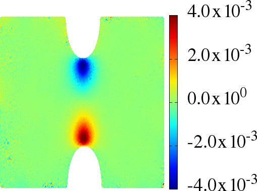
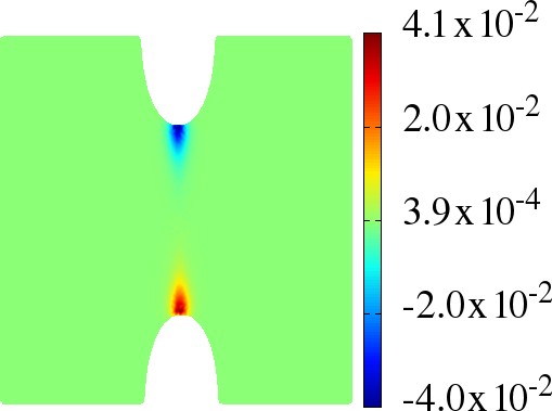
Figure 2: (Color online) – A geometrically stabilized domain wall in a non-convex domain, at $T/T_{c}=0.8$ for the parameter set I. The domain wall is geometrically trapped, since to escape it should increase its length, which is energetically costly. The phase difference $\varphi_{12}$ show that during the cooling, domain walls were created and one has been stabilized by the sample’s geometry. The unfavourable phase differences at the domain wall affects the densities of the condensates. $|\psi_{1}|^{2}$ overshoots at the domain wall, while $|\psi_{2}|^{2}$ and $|\psi_{3}|^{2}$ are depleted. Note that the domain wall has a magnetic signature: spots of the dipole-like magnetic field, where the domain wall touches the bumps. It originates in features of the interband counterflow at the domain wall, discussed in the text. The upper right panel shows the contribution to magnetic field of the second term in (Domain walls and their experimental signatures in $s+is$ superconductors).

While a frustrated superconductor is quenched through $T_{\mathbb{Z}_{2}}$, the temperature of the BTRS phase transition, domain walls are created. Because of their line tension, domain walls are unstable to be absorbed by the boundaries, or collapse if they are closed. Here we propose a mechanism for stabilization of domain walls, by using a geometric barrier. Such a barrier exists if a sample has a non-convex geometry as for example shown on Fig. 2. Next we will show, that when a domain wall is stabilized it has experimentally detectable features that can signal $s+is$ state. As shown in Fig. 2, if during a quench a domain wall ending on non-convex bumps is created, it can relax to a stable configuration.

  

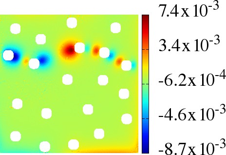
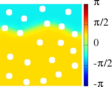
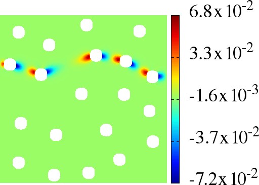
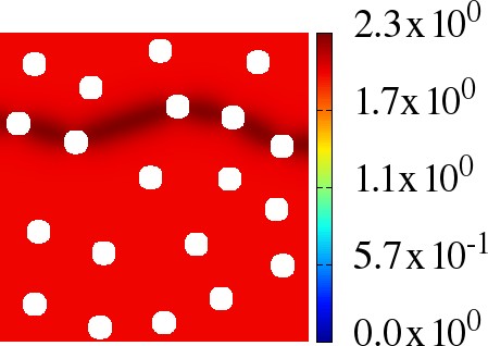
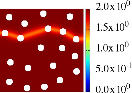
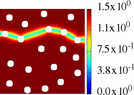
Figure 3: (Color online) – A domain wall stabilized by randomly located pinning centers. When cooled past $T_{\mathbb{Z}_{2}}$, domain walls are formed at random positions. Then, during the relaxation process, the quench-induced domain wall is stabilized against collapse by nearby pinning centers. Displayed quantities and physical parameters are the same as in Fig. 2. Here again, the domain wall has a dipole-like signature of the magnetic field where it is attached to the pinning centers.

Indeed, to join its ends and collapse to zero size, the domain wall would have to increase its length first, it is thus in a stable equilibrium while trapped on the bumps. Exactly the same effect is present when there is a pinning by inhomogeneities instead of a geometric barrier (see Fig. 3). This kind of pinning induces similar magnetic dipole signatures.

To simulate the cooling experiment, the energy is minimized at $T=T_{c}+\delta T$, i.e. starting in the normal state. The temperature is subsequently decreased with a step $\delta T$ and the energy minimized for the new temperature (i.e. new $\alpha_{a}$’s). The faster the system undergoes a phase transition, the more defects are nucleated. This is achieved, in our simulations, by cooling with bigger temperature steps (see animations in Sup for a typical domain wall-stabilizing process). Domain walls are always created, but their location is random and thus they do not always geometrically stabilize. We performed several simulations of the cooling processes and verified that indeed the number of produced defects is larger when temperature steps are bigger. Conversely, to ensure that no DW is formed, the system has to be cooled very slowly.

Remarkably, as shown in Figs. 2 and 3, even in zero applied field the domain wall carries opposite, non-zero magnetic field at its ends. Yet the total net flux through the sample is zero. The magnitude of this effect depends on the width of the domain wall (and thus on the parameters of the model). For Fig. 2, the amplitude of the local fields is of the order of magnitude of a percent of the magnetic field of a vortex. The origin of this signature in $s+is$ state is principally different from magnetic signature of domain walls in $p+ip$ superconductor. Namely, in $p+ip$ superconductors, DW carry uniform magnetic field originating from orbital momentum of Cooper pairs (see e.g. Ferguson and Goldbart (2011); Raghu et al. (2010); Vadimov and Silaev (2013)). Here, by contrast, the domain walls carry magnetic field only where they are attached to the boundary and the field inverts its direction so that there is no net flux. This magnetic field originates in interband counterflow in the presence of relative density gradients. Indeed, the magnetic field has the following dependence on the field gradients Garaud et al. (2013):

$$B_{z} =-\epsilon_{ij}\partial_{i}\left(\frac{J_{j}}{e^{|}\Psi|^{2}}\right)$$

$$-\frac{i\epsilon_{ij}}{e^{2}|\Psi|^{4}}\left[|\Psi|^{2}\partial_{i}\Psi^{\dagger}\partial_{j}\Psi+\Psi^{\dagger}\partial_{i}\Psi\partial_{j}\Psi^{\dagger}\Psi\right]\,,$$ (2)

with $\Psi^{\dagger}=(\psi_{1}^{*},\psi_{2}^{*},\psi_{3}^{*})$ and $|\Psi|^{2}=\Psi^{\dagger}\Psi$. The interband counterflow contribution to ${\boldsymbol{B}}$ is the second term (Domain walls and their experimental signatures in $s+is$ superconductors). That is, density gradients mixed with gradients of phase differences (see Figs. 2 and 3). In the total magnetic field signature, counterflows are partially screened by the first term.

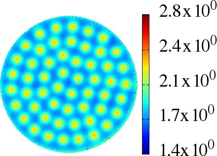
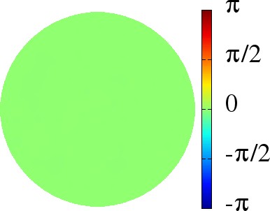
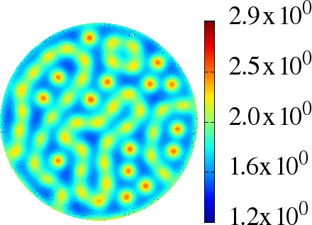
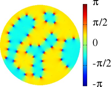
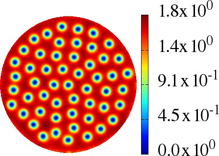
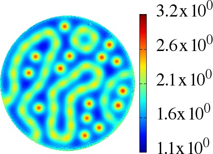
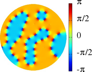
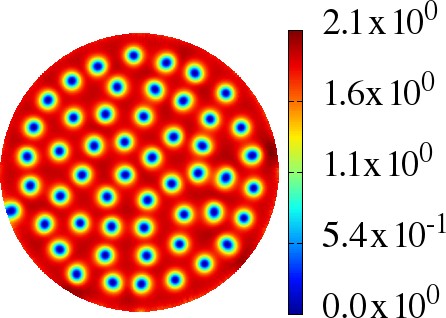
Figure 4: (Color online) – Field cooled experiment for the parameter set II, under an applied field $H/\Phi_{0}S=70$. First the system is a two-band ($\psi_{2}=0$) and thus it is TRS. Then when cooled through $T_{\mathbb{Z}_{2}}$ ($\psi_{2}\neq 0$) the system enters the BTRS regime and different region pick up different ground state phase-locking. The resulting DW are stabilized against complete contraction by the already existing vortices.

For modeling a field cooled experiment, the Gibbs energy for a given applied field $H$ is minimized for decreasing temperatures. This is shown in Fig. 4. At $T_{c}$ superconductivity sets in and the sample is filled with vortices. Then while temperature is further decreased, past $\ \mathbb{Z}_{2}\$phase transition (at $T_{\mathbb{Z}_{2}}$), KZ mechanism leads to the formation of domain walls. As shown in Fig. 4, the pre-existing vortices stabilize the domain wall against collapse (regardless of the geometry). These domain walls either terminate on the boundary or are closed. Closed domain walls stabilized by vortices were considered in Garaud et al. (2011, 2013). These are Skyrmions since they are characterized by $\ {\mathbbm{C}{P}}^{2}\$topological invariant. Note that to accommodate the unfavourable phase differences at the DW, it is beneficial to split vortices into three types of fractional vortices (see detailed discussion in Garaud et al. (2011, 2013)). Since at the DW, there is less total density, the penetration length is effectively smaller and vortices appear bigger. The DW can clearly be identified when measuring the magnetic field.

Consider now magnetization process at fixed $T<T_{\mathbb{Z}_{2}}$. No field is initially applied ($H=0$) and the superconductor is in one ground state. The applied field is increased with a step $\delta H$. There are no preexisting DW and, as long as the applied field is below $\ \mathrm{H}_{c1}\$, no vortex enters the system. The Meissner state survives to fields higher than $\ \mathrm{H}_{c1}\$because of the Bean-Livingston barrier. While the applied field is further increased, vortices enter and arrange in a triangular lattice. Note that, big steps $\delta H$ can provide enough energy to locally fall into the opposite $\ \mathbb{Z}_{2}\$state during a relaxation process. This thus leads to the formation of a domain wall which is stabilized by the presence of vortices (see Sup ).

Now we consider the regime of our main interest. As shown in Fig. 5, the magnetization process in the presence of quench-induced and geometrically stabilized domain wall is very unusual. Since some density components are depleted at the domain wall (see Fig. 2), vortex entry for the corresponding component costs much less energy there than from the boundaries. The first vortex entry occurs at much lower fields than $\ \mathrm{H}_{c1}\$. Here, a core is created only in one band, thus it is a fractional vortex which enters the domain wall. Fractional vortices are thermodynamically unstable in a uniform bulk superconducting state because they have logarithmically divergent energy Garaud et al. (2013). The situation here is different because the sample has a pre-existing domain wall. See Sup for all quantities. In increased field the domain wall is filled with vortices. Despite its energy cost, it eventually becomes beneficial to elongate the domain wall. It starts bending and gradually fills the sample. At the first integer vortex entry, the sample is already filled with the flux-carrying DW. The associated magnetization curves also show striking differences from the case without domains-wall. This can provide a way to confirm $s+is$ superconductivity. For a sample whose geometry allows stabilization of DW, magnetization process after a rapid cooling (or other kind of thermal quench) can be significantly different from that of the same, slowly cooled sample. The first will show magnetization process different from the reference measurement. Chances to stabilize domain walls are further enhanced by having multiple stabilizing geometric barriers.

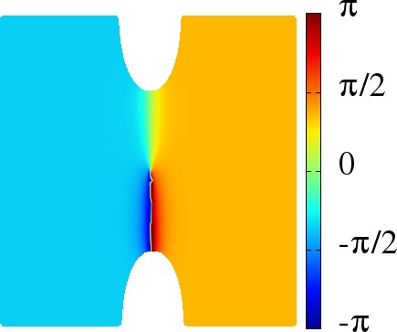
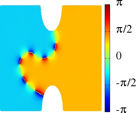
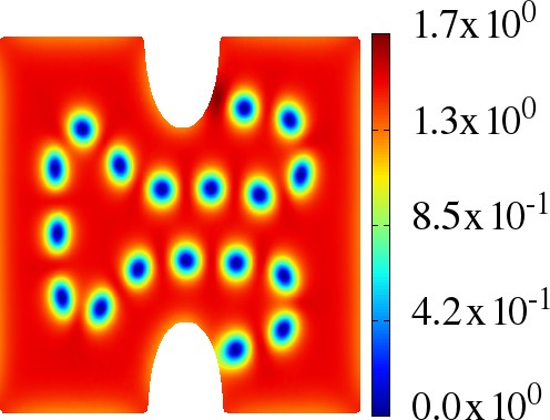
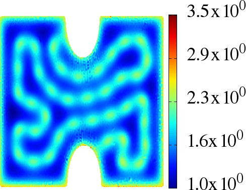
Figure 5: (Color online) – Magnetization process of a three-band BTRS, when the zero field configuration has the geometrically stabilized domain wall Fig. 2 (all parameters being the same). First vortex entry, way below $\ \mathrm{H}_{c1}\$, shown in the top row is a fractional vortex in $\psi_{3}$. This can be seen from the phase difference $\varphi_{13}$ which winds $2\pi$. The red curve is the magnetization curve of this process, while the blue curve is a reference magnetization, starting from a uniform ground state.

In conclusion, we have studied domain walls in $s+is$ superconductors. We presented proposal for an experimental set-up which can lead to formation of stable domain walls. We demonstrated that domain walls in $s+is$ superconductors have magnetic signatures which could be detected in scanning SQUID, Hall, or magnetic force microscopy measurements. Moreover we showed that for geometrically stabilized DW, the magnetization curve could change substantially as DW allows flux penetration in the form of fractional vortices in low fields. Thus a sample subject to different cooling processes should exhibit very different magnetization process and magnetization curves.

The observation of these features can signal $s+is$ state (because in contrast $s_{\pm}$ and $s_{++}$ states do not break $\ \mathbb{Z}_{2}\$symmetry and thus have no domain walls), for example in hole-doped Ba_1-xK_xFe₂As₂ Maiti and Chubukov (2013).

Appendix B Phase diagram in the Ginzburg-Landau regime

For our purposes, we do not need to reproduce phase diagram of Maiti and Chubukov (2013) quantitatively. It is sufficient, to retain temperature dependency only of the following coefficients:

$$\alpha_{a}\equiv\alpha_{a}(T)=\alpha^{(0)}_{a}\ln\frac{T}{T_{a}}\simeq\alpha^{(0)}_{a}\left(\frac{T}{T_{a}}-1\right)\,.$$ (B.1)

The temperatures are scaled so that in zero applied field, $T_{c}=1$. We investigate only a restricted range of temperatures $T/T_{c}\in[0.8;1]$. Figures 6 and 7 display the $H/T$ diagram for the parameter sets studied in the main text. The actual values of the parameters are given in the captions. In the main text, we discuss two possible routes to break time-reversal symmetry during the cooling process. Such a phase diagram agrees with microscopic calculations Maiti and Chubukov (2013) and is reproduced here phenomenologically in the framework of a minimal Ginzburg-Landau model.

Figure 6: (Color online) – Phase diagram and ground state configuration for the parameter set I. That is, the Ginzburg-Landau parameters are $(\alpha^{(0)}_{1},\alpha^{(0)}_{2},\alpha^{(0)}_{3})=(8.273,10.412,8.5)$ and $(T_{1},T_{2},T_{3})=(0.91,0.885,0.85)$. The gauge coupling $e=0.3$, while $\beta_{a}=1$ and $\eta_{12}=\eta_{13}=-\eta_{23}=2$.

For the first symmetry breaking pattern, which we refer as set I, superconductivity arises for all three-bands below $T_{c}$. The frustration becomes important enough to break time-reversal symmetry only below $T_{\mathbb{Z}_{2}}<T_{c}$. Thus before reaching the BTRS state, the system is a three-band TRS superconductor (the $s_{++}$ state). The related phase diagram is displayed in Fig. 6. The second symmetry breaking pattern which we investigate, shown in Fig. 7 is different. For temperatures $T_{\mathbb{Z}_{2}}<T<T_{c}$, only two bands develop superconductivity (the $s_{\pm}$ state). There thus is only one Josephson term, and the phases are trivially locked. Below $T_{\mathbb{Z}_{2}}$, the third condensate becomes superconducting and the time-reversal symmetry is broken (the $s+is$ state) because all three (frustrated) Josephson terms are important enough.

Note that at $T=0.8$, the values of the parameters of the Ginzburg-Landau functional are the same for parameter sets I and II. The magnetization process at $T=0.8$ is thus the same for both these systems.

Figure 7: (Color online) – Phase diagram and ground state configuration for the parameter set II. That is, the Ginzburg-Landau parameters are $(\alpha^{(0)}_{1},\alpha^{(0)}_{2},\alpha^{(0)}_{3})=(11.8108,41,4.9444)$ and $(T_{1},T_{2},T_{3})=(0.874,0.82,0.89)$. The gauge coupling $e=0.3$, while $\beta_{a}=1$ and $\eta_{12}=\eta_{13}=-\eta_{23}=2$.

Appendix C Finite element energy minimization

We consider the two-dimensional problem is defined on the bounded domain $\Omega\subset\mathbbm{R}^{2}$ with $\partial\Omega$ its boundary. $\Omega$ can assume any geometry. In particular, it can be convex (homeomorph to a disc) or non-convex. The problem is supplemented by the boundary condition ${\boldsymbol{n}}\cdot{\boldsymbol{D}}\psi_{a}=0$ with ${\boldsymbol{n}}$ the normal vector to $\partial\Omega$. Physically this condition implies there is no current flowing through the boundary. A superconductor subject to an external field ${\boldsymbol{H}}=H\boldsymbol{e}_{z}$ is described by the Gibbs free energy $\mathcal{G}=\mathcal{F}-{\boldsymbol{B}}\cdot{\boldsymbol{H}}$, yielding the boundary conditions on $\partial\Omega$ for the vector potential $\boldsymbol{\nabla}\times{\boldsymbol{A}}={\boldsymbol{H}}$.

The variational problem is defined for numerical computation using a finite element formulation provided by the Freefem++ library Hecht et al. (2007). Discretization within finite element formulation is done via a (homogeneous) triangulation over $\Omega$, based on Delaunay-Voronoi algorithm. Functions are decomposed on a continuous piecewise quadratic basis over each triangle. The accuracy of such method is controlled through the number of triangles, (we typically used $3\sim 6\times 10^{4}$), the order of expansion of the basis on each triangle (2nd order polynomial basis on each triangle), and also the order of the quadrature formula for the integral on the triangles.

Once the problem is posed, a numerical optimization algorithm is used to solve the variational non-linear problem (i.e. to find the minima of $\mathcal{G}$). We used here a non-linear conjugate gradient method. The algorithm is iterated until relative variation of the norm of the gradient of the functional $\mathcal{G}$ with respect to all degrees of freedom is less than $10^{-6}$.

C.1 Field cooled experiments

Simulating a field cooled experiment, is done through the following sequences. For a given value of the applied field $H$, the initial temperature is chosen so that it slightly exceeds the second critical field ($H>\mathrm{H}_{c2}$). Then the Gibbs energy is minimized for a given temperature. For the next step the temperature is decreased by step $\delta T$ and the Gibbs energy is subsequently minimized using solution at the previous temperature as an initial guess. To ensure that the system is not trapped into an artificial minimum, a small white noise corresponding to small thermal fluctuations is added at each temperature step, before further relaxing the energy. This procedure, corresponds to an horizontal path in the $H(T)$ diagram. It is iterated down to a given temperature, which we chose to be $T_{min}=0.8T_{c}$.

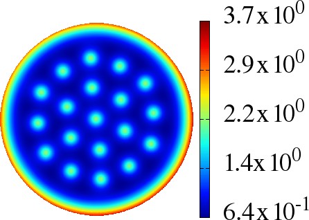
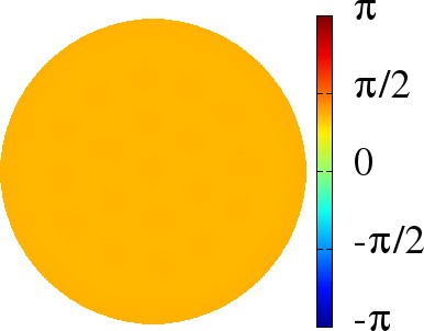
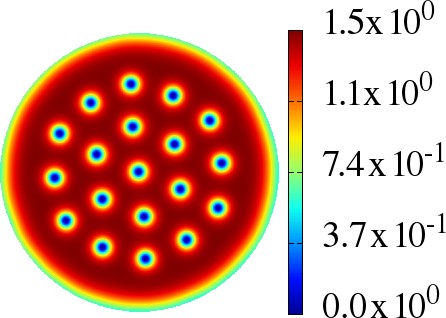
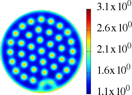
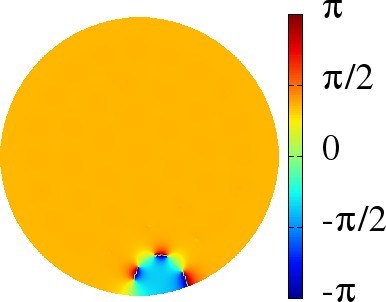
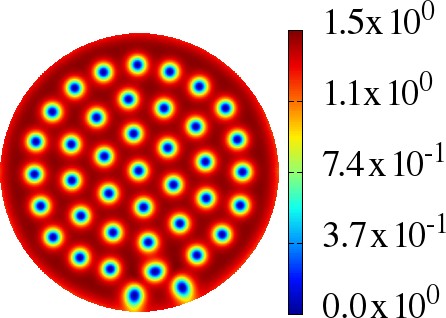
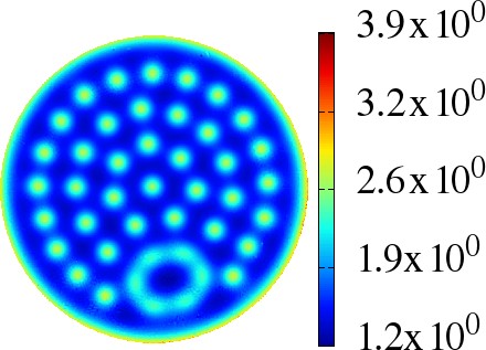
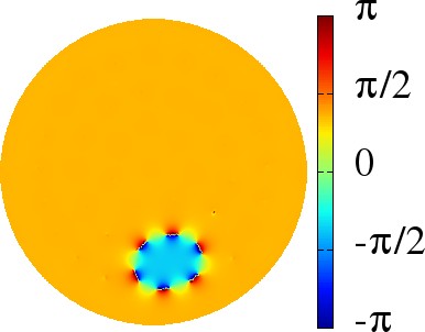
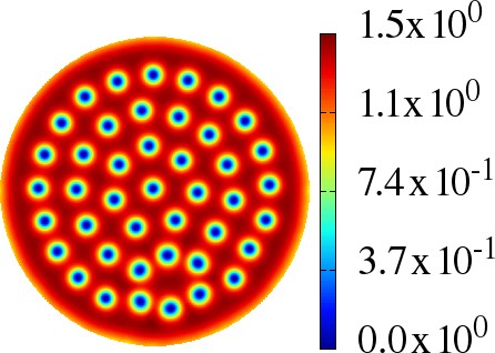
Figure 8: (Color online) – Magnetization process of a three-band superconductor in the BTRS state. As the domain is convex, the zero field configuration has no domain wall. Increase of the applied field can lead the system to locally fall into the opposite $\ \mathbb{Z}_{2}\$state and seeds a domain wall. The latter is stabilized by the vortices as in Fig. 3 of the paper. The parameter are the same as in Fig. 2 of the main text.

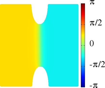
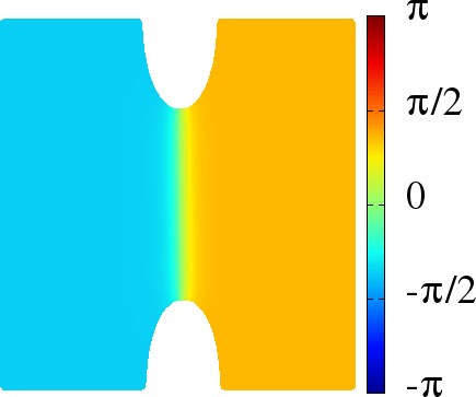
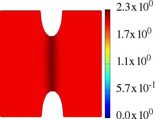
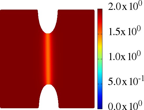
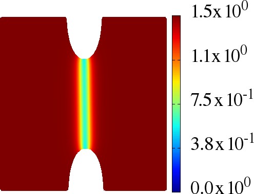
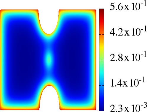
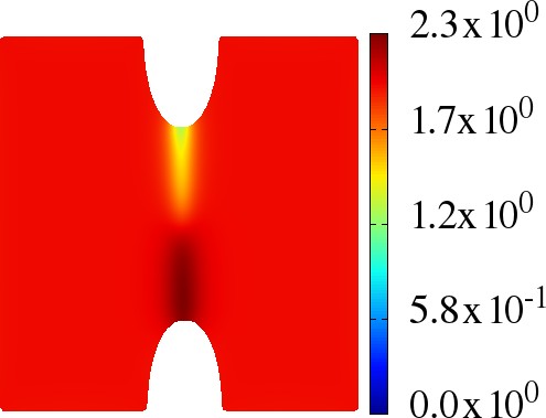
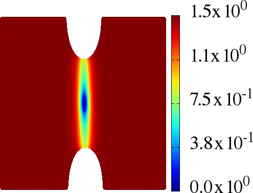
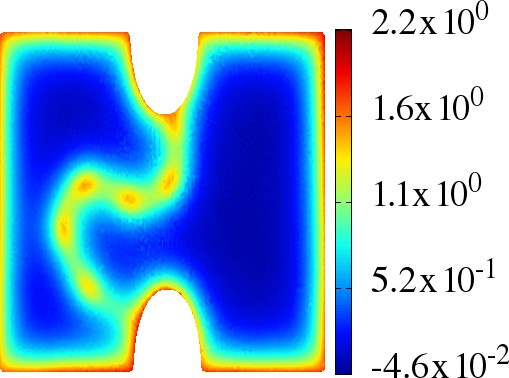
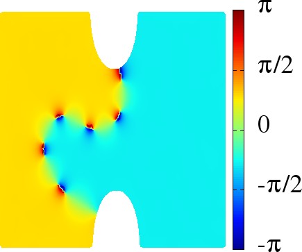
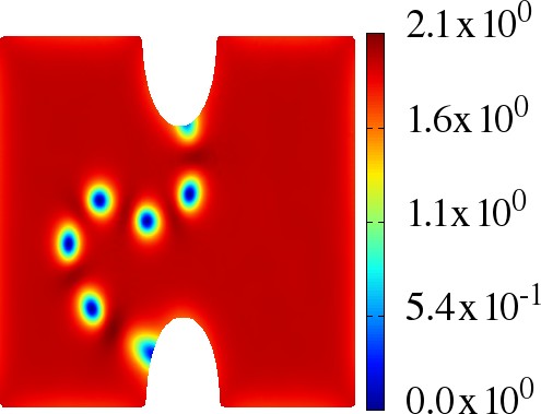
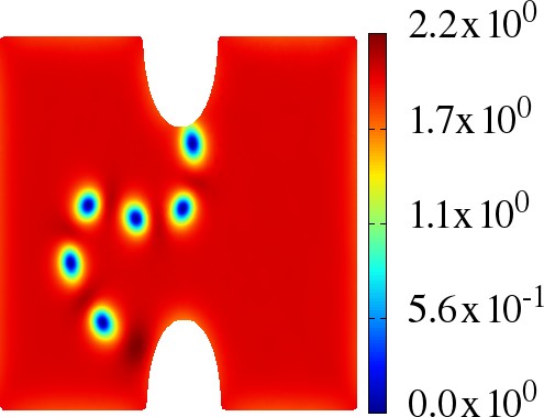
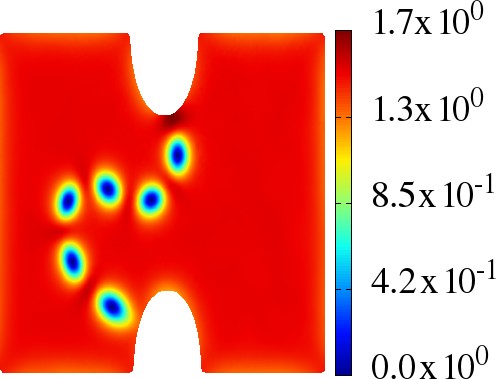
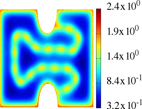
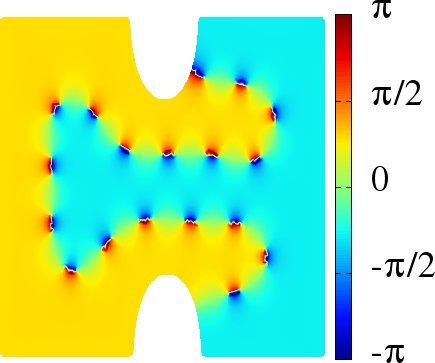
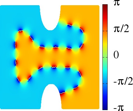
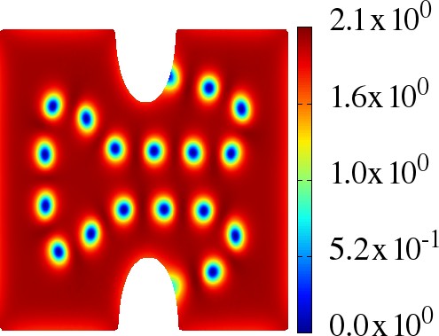
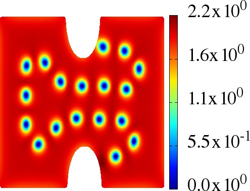
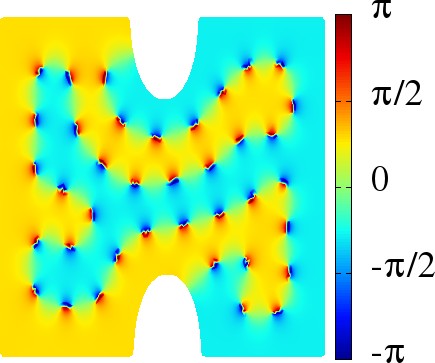
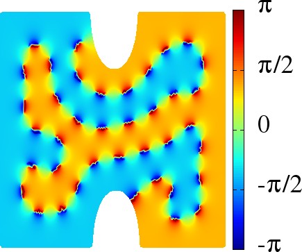
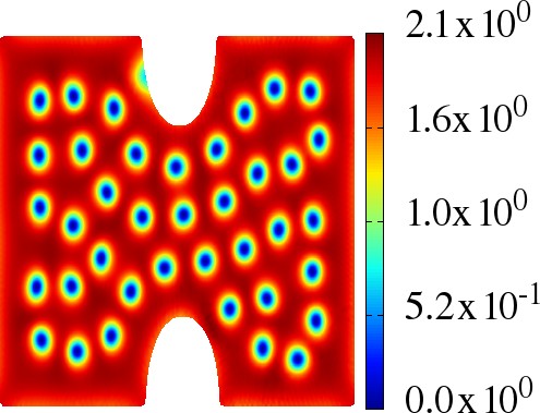
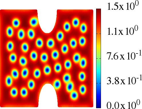
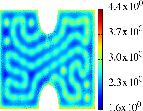
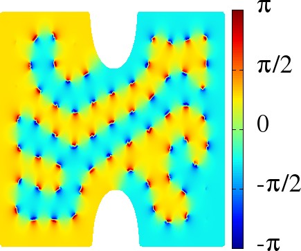
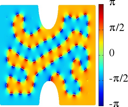
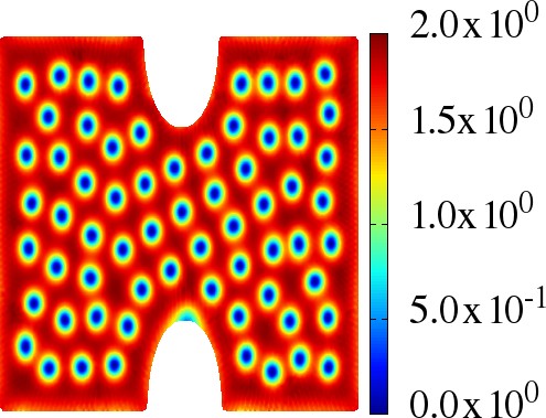
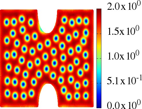
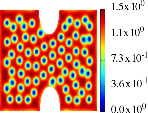
Figure 9: (Color online) – Magnetization process of a three-band BTRS, when the zero field configuration has the geometrically stabilized domain wall This displays additional quantities to the magnetization process shown in Fig. 4 of the main text. First vortex entry, way below $\ \mathrm{H}_{c1}\$, shown in the second row is a fractional vortex in $\psi_{3}$. This can be seen from the phase difference $\varphi_{13}$ which winds $2\pi$ and that $|\psi_{1}|^{2}$ and $|\psi_{2}|^{2}$ have no singularity.

Physically, this correspond to start the experiment with some applied field ${\boldsymbol{H}}$ at a temperature above the critical temperature. That is, initially there is no superconducting state. Then while decreasing the temperature, normal state is no longer stable and the system goes to superconducting state with vortices (when there is a non-zero applied field). While cooled, the system goes across the BTRS transition at $T_{\mathbb{Z}_{2}}$. There, different regions can fall into different ground states, thus leading to domain wall formation. This is Kibble-Zurek mechanism. Note that KZ mechanism involves actual time dependence. In our approach, we use a minimization algorithm instead of solving the actual time-dependent equations. At each temperature, once the algorithm has converged, the system is stationary. Thus we do not simulate the actual dynamics of Kibble-Zurek. Rather it is a quasi-equilibrium process which mimics the KZ mechanism.

C.2 Magnetization process at fixed $T$.

This experiment investigates the response of the superconductor of an applied external field, at a fixed temperature. Below its critical temperature, no field is initially applied ($H=0$). The $H=0$ configuration is generated by cooling the sample from $T_{c}$ to a preferred temperature below $T_{\mathbb{Z}_{2}}$. Thus, during the cooling process domain walls have been created. For a convex geometry, they can always decay to zero, while they can be geometrically stabilized, for non-convex geometries. For the magnetization process, the superconductor is initially either in the uniform ground state or non-uniform in the presence of a domain wall.

Then keeping the temperature fixed, the applied field is increased with a step $\delta H$. The configuration of the condensates and vector potential of the previous step is used and Gibbs energy minimized for the new value of the applied field. This corresponds physically to apply an increasing magnetic field at fixed temperature. As long as the applied field is below $\ \mathrm{H}_{c1}\$, it is not energetically preferable to nucleate flux carrying topological defects and the superconductor stays in the Meissner state. Above $\ \mathrm{H}_{c1}\$topological defects start to enter the system. Actually first vortex entry occurs for higher values of the applied field, since they have to overcome the Bean-Livingston barrier which depends on the geometry.

Big steps $\delta H$ in the applied field, can provide enough energy to locally fall into the opposite $\ \mathbb{Z}_{2}\$state during a relaxation process. As seen in Fig. 8, this thus leads to the formation of a domain wall which is stabilized by the presence of vortices.

Additional quantities, to the unusual magnetization process in presence of a domain wall in zero applied field are displayed in Fig. 9.