On Schwarz Methods for Nonsymmetric and Indefinite Problems

Abstract

In this paper we introduce a new Schwarz framework and theory, based on the well-known idea of space decomposition, for nonsymmetric and indefinite linear systems arising from continuous and discontinuous Galerkin approximations of general nonsymmetric and indefinite elliptic partial differential equations. The proposed Schwarz framework and theory are presented in a variational setting in Banach spaces instead of Hilbert spaces which is the case for the well-known symmetric and positive definite (SPD) Schwarz framework and theory. Condition number estimates for the additive and hybrid Schwarz preconditioners are established. The main idea of our nonsymmetric and indefinite Schwarz framework and theory is to use weak coercivity (satisfied by the nonsymmetric and indefinite bilinear form) induced norms to replace the standard bilinear form induced norm in the SPD Schwarz framework and theory. Applications of the proposed nonsymmetric and indefinite Schwarz framework to solutions of discontinuous Galerkin approximations of convection-diffusion problems are also discussed. Extensive 1-D numerical experiments are also provided to gauge the performance of the proposed Schwarz methods.

1 Introduction

The original Schwarz method, proposed and analyzed by Hermann Schwarz in 1870 [26], is an iterative method to find the solution of a partial differential equation (PDE) on a complicated domain which is the union of two overlapping simpler subdomains. The method solves the equation on each of the two subdomains by using the latest values of the approximate solution as the boundary conditions on the parts of the subdomain boundaries which are inside of the given domain. The idea of splitting a given problem posed on a large (and possibly complicated) domain into several subproblems posed on smaller subdomains and then solving the subdomain problems either sequentially or in parallel is a very appealing idea. Such a “divide-and-conquer” idea is at the heart of every domain decomposition or Schwarz method.

It is well-known that [27] the domain decomposition strategy can be introduced at the following three different levels: the continuous level for PDE analysis as proposed and analyzed by Hermann Schwarz in 1870, the discretization level for constructing (hybrid and composite) discretization methods, and the algebraic level for solving algebraic systems arising from the numerical approximations of PDE problems. These three levels are often interconnected, and each of them has its own merit to be studied. Most of the recent efforts and attentions have been focused on the algebraic level. The field of domain decomposition methods has blossomed and undergone intensive and phenomenal development during the last thirty years (cf. [25, 22, 27] and the references therein). The phenomenal development has largely been driven by the ever increasing demands for fast solvers for solving important and complicated scientific, engineering and industrial application problems which are often governed mathematically by a PDE or a system of PDEs. It has also been infused and facilitated by the rapid advances in computer hardware and the emergence of parallel computing technologies.

At the algebraic level, domain decomposition methods or Schwarz methods have been well developed and studied for various numerical approximations (discretizations) of many types of PDE problems including finite element methods (cf. [12, 29]), mixed finite element methods and spectral methods (cf. [27]), and discontinuous Galerkin methods (cf. [14, 20, 15, 2]). A general abstract framework, backed by an elegant convergence theory, was well established many years ago for symmetric and positive definite (SPD) PDE problems and their numerical approximations (cf. [12, 29, 25, 22, 27, 30] and the references therein).

Despite the tremendous advances in domain decomposition (Schwarz) methods over the past thirty years, the current framework and convergence theory are mainly confined to SPD problems in Hilbert spaces. Because the framework and especially the convergence theory indispensably rely on the SPD properties of the underlying problem and the Hilbert space structures, they do not apply to genuinely nonsymmetric and/or indefinite problems. As a result, the SPD framework and theory leave many important and interesting problems uncovered as pointed out in [27, page 311].

This paper attempts to address this important issue in Schwarz methods. The goal of this paper is to introduce a new Schwarz framework and theory, based on the well-known idea of space decomposition as in the SPD case, for nonsymmetric and indefinite linear systems arising from continuous and discontinuous Galerkin approximations of general nonsymmetric and indefinite elliptic partial differential equations under some “minimum” structure assumptions. Unlike the SPD framework and theory, our new framework and theory are presented in a variational setting in Banach spaces instead of Hilbert spaces. Such a general framework allows broader applications of Schwarz methods. Both additive Schwarz and multiplicative as weel as hybrid Schwarz methods are developed. A comprehensive convergence theory is provided which includes condition number estimates for the additive Schwarz preconditioners and hybrid Schwarz preconditioners. The main idea of our nonsymmetric and indefinite Schwarz framework and theory is to use weak coercivity (satisfied by the nonsymmetric and indefinite bilinear form) induced norms to replace the standard bilinear form induced norm in the SPD Schwarz framework and theory (see Sections 2–4 for a detailed exposition). As expected, working with such weak coercivity induced norms and nonsymmetric and indefinite bilinear forms is quite delicate. It requires new and different technical tools in order to establish our convergence theory.

The remainder of this paper is organized in the following way. In Section 2, we introduce notation, the functional setting, and the variational problems which we aim to solve. Section 2 also contains some further discussions on the main idea of the paper. Section 3 is devoted to establishing an abstract additive Schwarz, multiplicative Schwarz, and hybrid Schwarz framework for general nonsymmetric and indefinite algebraic problems in a variational setting in general Banach spaces. In Section 4, we present an abstract convergence theory for the additive and hybrid Schwarz methods proposed in Section 3. In Section 5, we present some applications of the proposed nonsymmetric and indefinite Schwarz framework to discontinuous Galerkin approximations of convection-diffusion (in particular, convection-dominated) problems. We also provide extensive 1-D numerical experiments to gauge the performance of the proposed nonsymmetric and indefinite Schwarz methods.

2 Functional setting and statement of problems

2.1 Variational problem

Let $X$ be a real Hilbert space with the inner product $(\cdot,\cdot)_{X}$ and the induced norm $\|\cdot\|_{X}$. Let $V,W\subset X$ be two reflexive Banach spaces endowed with the norms $\|\cdot\|_{V}$ and $\|\cdot\|_{W}$ respectively. Let $\mathcal{A}(\cdot,\cdot)$ be a real bilinear form defined on the product space $V\times W$ and $\mathcal{F}$ be a real linear functional defined on $W$. We consider the following variational problem: Find $u\in V$ such that

(1) $$\mathcal{A}(u,w)=\mathcal{F}(w)\qquad\forall w\in W.$$

The well-posedness of the above variational problem has been extensively studied. One of such results is summarized in the following theorem:

Theorem 1.

(cf. [4]) Suppose that $\mathcal{F}$ is a bounded linear functional on $W$. Assume that $\mathcal{A}(\cdot,\cdot)$ is continuous and weakly coercive in the sense that there exist constants $C_{\mathcal{A}},\gamma_{\mathcal{A}}>0$ such that

(2) $$|\mathcal{A}(v,w)| \leq C_{\mathcal{A}}\|v\|_{V}\|w\|_{W} \qquad\forall v\in V,\,w\in W,$$

(3) $$\sup_{w\in W}\frac{\mathcal{A}(v,w)}{\|w\|_{W}} \geq\gamma_{\mathcal{A}}\|v\|_{V} \qquad\forall v\in V,$$

(4) $$\sup_{v\in V}\mathcal{A}(v,w) >0 \qquad\forall\,0\neq w\in W.$$

Then problem (1) has a unique solution $u\in V$. Moreover,

(5) $$\|u\|_{V}\leq\frac{\|\mathcal{F}\|}{\gamma_{\mathcal{A}}}.$$

Remark 2.1.

(a) Theorem 1 is called Lax-Milgram-Babuška theorem in the literature (cf. [24]). It was first introduced to the finite element context in [3] (also see [4]). An earlier version of the theorem can also be found in [21].

(b) As pointed out in [4, page 117], condition (4) can be replaced by the following more restrictive condition: There exists a constant $\beta_{\mathcal{A}}>0$ such that

(6) $$\sup_{v\in V}\frac{\mathcal{A}(v,w)}{\|v\|_{V}}\geq\beta_{\mathcal{A}}\|w\|_{W}\qquad\forall w\in W.$$

The above condition can be viewed as a weak coercivity condition for the adjoint bilinear form $\mathcal{A}^{*}(\cdot,\cdot)$ of $\mathcal{A}(\cdot,\cdot)$.

(c) Weak coercivity condition (3) is often called the inf-sup or Babuška–Brezzi condition in the finite element literature [7, 11] for a different reason. It appears and plays a vital role for saddle point problems and their (mixed) finite element approximations (cf. [8, 9]).

(d) Theorem 1 is certainly valid when $V=W$. Since condition (3) is weaker than the strong coercivity, then Theorem 1 is a stronger result than the classical Lax-Milgram Theorem for the case $V=W$. Indeed, for most convection-dominated convection-diffusion problems, $V=W$. However, there are situations where condition (3) holds but strong coercivity fails.

(e) There are also situations where one prefers to use different norms for the trial space $V$ and the test space $W$ even if $V=W$. Theorem 1 also provides a convenient framework to handle such a situation.

2.2 Discrete problem

As problem (1) is posed on infinite dimensional spaces $V$ and $W$, to solve it numerically, one must approximate $V$ and $W$ by some finite dimensional spaces $V_{n},W_{n}\subset X$. Here $n=\mbox{dim}(V_{n})=\mbox{dim}(W_{n})$ is a positive integer which denotes the dimension of $V_{n}$ and $W_{n}$. If one of (or both) $V_{n}$ and $W_{n}$ is not a subspace of its corresponding infinite dimensional space, then one also needs to provide an approximate bilinear form $a(\cdot,\cdot)$ for $\mathcal{A}(\cdot,\cdot)$ so that $a(\cdot,\cdot)$ is well defined on $V_{n}\times W_{n}$. In addition, if $W_{n}$ is not a subspace of $W$ one also needs to provide an approximate linear functional $f$ for $\mathcal{F}$ so that $f$ is well defined on $W_{n}$.

Once $V_{n},W_{n},a$ and $f$ are constructed, the Galerkin method for problem (1) is defined as seeking $u_{n}\in V_{n}$ such that

(7) $$a(u_{n},w_{n})=f(w_{n})\qquad\forall w_{n}\in W_{n}.$$

Pick a basis $\{\phi^{(j)}\}_{j=1}^{n}$ of $V$ and a basis $\{\psi^{(j)}\}_{j=1}^{n}$ of $W$. It is trivial to check that the discrete variational problem (7) can be rewritten as the following linear system problem:

(8) $$A\mathbf{u}=\mathbf{f},$$

where $\mathbf{u}=[u^{(j)}]_{j=1}^{n}$ is the coefficient vector of the representation of $u_{n}$ in terms of the basis $\{\phi^{(j)}\}_{j=1}^{n}$ and

(9) $$A =\bigl{[}a_{ij}\bigr{]}_{i,j=1}^{n}, \qquad a_{ij} =a(\phi^{(j)},\psi^{(i)}),$$

(10) $$\mathbf{f} =\bigl{[}f^{(i)}\bigr{]}_{i=1}^{n}, \qquad f^{(i)} =f(\psi^{(i)}).$$

The properties of matrix $A$ (called a stiffness matrix) are obviously determined by the properties of the discrete bilinear form $a(\cdot,\cdot)$ and the approximate spaces $V_{n}$ and $W_{n}$. When $V_{n}=W_{n}$ it is well known that [17] $A$ is symmetric if and only if $a(\cdot,\cdot)$ is symmetric and $A$ is positive definite provided that $a(\cdot,\cdot)$ is strongly coercive on $V_{n}\times V_{n}$. In general, $A$ is just an $n\times n$ nonsymmetric real matrix if $a(\cdot,\cdot)$ is not symmetric. $A$ also can be indefinite (i.e., $A$ has at least one negative and one positive eigenvalue) if $a(\cdot,\cdot)$ fails to be coercive.

As (8) is a square linear system, by a well-known algebraic fact we know that (8) has a unique solution $\mathbf{u}$ provided that the stiffness matrix $A$ is nonsingular. This nonsingular condition on $A$ becomes necessary if one wants (8) to be uniquely solvable for arbitrary vector $\mathbf{f}$. For most application problems (such as boundary value problems for elliptic PDEs), one needs to consider various choices of the “load” functional $\mathcal{F}$, so the vector $\mathbf{f}$ is practically “arbitrary” in (8). Hence, besides some deeper mathematical and algorithmic considerations, asking for the stiffness matrix $A$ to be nonsingular is a “minimum” requirement for the discretization method (7) to be practically useful.

Sufficient conditions on the discrete bilinear form $a(\cdot,\cdot)$ and the approximate spaces $V_{n}$ and $W_{n}$ which infer the unique solvability of the linear system (8) have been well studied and understood in the past thirty years. In particular, for the SPD type (algebraic) problems arising from various discretizations of boundary value problems for elliptic PDEs [3, 4, 11, 7, 4, 5, 23]. In the following we shall quote some of these well-known results in a theorem which is a counterpart of Theorem 1.

Theorem 2.

(cf. [3, 4]) Suppose that $f$ is a bounded linear functional on $W_{n}$. Assume that $a(\cdot,\cdot)$ is continuous and weakly coercive in the sense that there exist constants $C_{a},\gamma_{a},\beta_{a}>0$ such that

(11) $$|a(v,w)| \leq C_{a}\|v\|_{V_{n}}\|w\|_{W_{n}} \qquad\forall v\in V_{n},\,w\in W_{n},$$

(12) $$\sup_{w\in W_{n}}\frac{a(v,w)}{\|w\|_{W_{n}}} \geq\gamma_{a}\|v\|_{V_{n}} \qquad\forall v\in V_{n},$$

(13) $$\sup_{v\in V_{n}}\frac{a(v,w)}{\|v\|_{V_{n}}} \geq\beta_{a}\|w\|_{W_{n}} \qquad\forall w\in W_{n}.$$

Then problem (7) has a unique solution $u_{n}\in V_{n}$. Moreover,

(14) $$\|u_{n}\|_{V_{n}}\leq\frac{M_{f}}{\gamma_{a}}$$

where $M_{f}$ is a positive constant.

A few remarks are in order about the above well-posedness theorem.

Remark 2.2.

(a) Condition (13) is equivalent to requiring that the adjoint $a^{*}(\cdot,\cdot)$ of $a(\cdot,\cdot)$ is weakly coercive.

(b) Conditions (11)–(13) are analogies of their continuous counterparts (2)–(4). Discrete weak coercivity condition (12) is often called the inf-sup or Babuška–Brezzi condition in the finite element literature [7, 11] for a different reason. It is the most important one in a set of sufficient conditions for a mixed finite element to be stable (cf. [8, 9]).

(c) A numerical method which fulfills conditions (11)–(13) is guaranteed to be uniquely solvable and stable. Hence, these conditions can be used as a test stone to determine whether a numerical method is a “good” method. For this reason, we shall call the numerical method (7) an inf-sup preserving method or a weak coercivity preserving method if it satisfies (11)–(13).

(d) Theorem 2 focuses on the unique solvability and the stability of the numerical method (7) not on the accuracy of the method. We like to note that method (7) indeed is an accurate numerical method provided that approximate spaces $V_{n}$ and $W_{n}$ are accurate approximations of $V$ and $W$ (cf. [4]).

2.3 Main objective

As we briefly explained above, approximating the variational problem (1) by a Galerkin method certainly results in solving the linear system (8). It is well known that the common dimension $n$ of the approximation spaces $V_{n}$ and $W_{n}$ has to be sufficiently large in order for the Galerkin method to be accurate. As a result, the size of the linear system (i.e., the size of the matrix $A$) is expected to be very large in applications. Moreover, if (1) is a variational formulation of some elliptic boundary value problem, then the stiffness matrix $A$ is certainly ill-conditioned in the sense that the condition number $\kappa(A):=\|A\|\|A^{-1}\|$ is very large. Here $\|A\|$ denotes a matrix norm of $A$. For example, in the case of second and fourth order elliptic boundary value problems, $\kappa(A)=O(n^{\frac{2}{d}})$ and $\kappa(A)=O(n^{\frac{4}{d}})$, respectively, where d is the spatial dimension of the domain. (cf. [7, 27]). Consequently, it is not efficient to solve linear system (8) directly using classical iterative methods even if they converge. Furthermore, unlike in the SPD case, classical iterative methods often do not converge for general nonsymmetric and indefinite linear system (8) (cf. [17, 27]).

As a first step toward developing better iterative solvers for nonsymmetric and indefinite linear system (8), it is natural to design a “good” preconditioner (i.e., an $n\times n$ real matrix $B$) such that $BA$ is well-conditioned (i.e., $\kappa(BA)$ is relatively small, say, significantly smaller than $\kappa(A)$). Then one can try classical iterative methods. In particular, the Generalized Minimal Residual (GMRES) method can be used on the preconditioned system

(15) $$BA\mathbf{x}=B\mathbf{b}.$$

One can also develop some new (and hopefully better) iterative methods if classical iterative methods still do not work as well on (15) as one had hoped.

As was already mentioned in Section 1, the focus of this paper is exactly what is described above. Our goal is to develop a new Schwarz framework and theory, based on the well-known idea of space decomposition, for solving nonsymmetric and indefinite linear system (8) which arises from the Galerkin method (7) as an approximation of the variational problem (1). As expected, our nonsymmetric and indefinite Schwarz framework and theory are natural extensions of the well-known SPD Schwarz framework and theory which were nicely described in [12, 29, 25, 22, 27].

3 An abstract Schwarz framework for nonsymmetric and indefinite problems

For the sake of notational brevity, throughout the remainder of this paper we shall suppress the sub-index $n$ in the discrete spaces $V_{n}$ and $W_{n}$ and in discrete functions $u_{n}$, $v_{n}$ and $w_{n}$. In other words, $V$ and $W$ are used to denote $V_{n}$ and $W_{n}$, and $u$, $v$ and $w$ are used to denote $u_{n}$, $v_{n}$ and $w_{n}$. In addition, we shall make an effort below to use the same or similar terminologies, as well as space and norm notation as those in [27] for the symmetric and positive definite (SPD) Schwarz framework and theory. We shall also make comments about notation and terminologies which have no SPD counterparts and try to make links between the well known SPD Schwarz framework and theory and our nonsymmetric and indefinite Schwarz framework and theory.

To motivate, we recall that in the SPD Schwarz framework and theory [12, 29, 25, 22, 27], since $V=W$ and the discrete bilinear form $a(\cdot,\cdot)$ is symmetric and strongly coercive, $\sqrt{a(v,v)}$ defines a convenient norm (which is also equivalent to the $\|\cdot\|_{V}$-norm) on the space $V$ (as well as on its subspaces). This bilinear form induced norm plays a vital role in the SPD Schwarz framework and theory.

Unfortunately, without the symmetry and strong coercivity assumptions on $a(\cdot,\cdot)$, $\sqrt{a(v,v)}$ is not a norm anymore when $V=W$. It is not even well defined if $V\neq W$! To overcome this difficulty, the existing nonsymmetric and indefinite Schwarz framework and theory (cf. [10, 27]), which only deal with the case $V=W$, assume that $a(\cdot,\cdot)$ has a decomposition $a(\cdot,\cdot)=a_{0}(\cdot,\cdot)+a_{1}(\cdot,\cdot),$ where $a_{0}(\cdot,\cdot)$ is assumed to be symmetric and strongly coercive (i.e., it is SPD) and $a_{1}(\cdot,\cdot)$ is a perturbation of $a_{0}(\cdot,\cdot)$. In this setting $a_{0}(\cdot,\cdot)$ then induces an equivalent (to $\|\cdot\|_{V}$) norm $\sqrt{a_{0}(v,v)}$ and one then works with this norm as in the SPD case. Unfortunately and understandably, such a setting requires that $a_{1}(\cdot,\cdot)$ is a small perturbation of $a_{0}(\cdot,\cdot)$, which is why the existing nonsymmetric and indefinite Schwarz framework and theory only apply to “nearly” SPD problems. Hence, it leaves more interesting and more difficult nonsymmetric and indefinite problems unresolved.

3.1 Main assumptions and main idea

To develop a new Schwarz framework and theory for general nonsymmetric and indefinite problems, our only assumptions on the discrete problem (7) are those stated in the well-posedness Theorem 2. We now restate those assumptions on the discrete bilinear form $a(\cdot,\cdot)$ and its adjoint $a^{*}(\cdot,\cdot)$ using the new function and space notation (i.e., after suppressing the sub-index $n$) as follows:

Main Assumptions

• Continuity There exists a positive constant $C_{a}$ such that

  (16) $$|a(v,w)|\leq C_{a}\|v\|_{V}\|w\|_{W}\qquad\forall v\in V,\,w\in W.$$

• Weak coercivity There exists positive constants $\gamma_{a}$, $\beta_{a}$ such that

  (17) $$\sup_{w\in W}\frac{a(v,w)}{\|w\|_{W}} \geq\gamma_{a}\|v\|_{V} \qquad\forall v\in V,$$

  (18) $$\sup_{v\in V}\frac{a(v,w)}{\|v\|_{V}} \geq\beta_{a}\|w\|_{W} \qquad\forall w\in W.$$

Remark 3.1.

(a) Since $a^{*}(w,v)=a(v,w)$, then the continuity condition (16) is equivalent to

(19) $$|a^{*}(w,v)|\leq C_{a}\|w\|_{W}\|v\|_{V}\qquad\forall w\in W,\,v\in V,$$

and (18) is equivalent to

(20) $$\sup_{v\in V}\frac{a^{*}(w,v)}{\|v\|_{V}}\geq\beta_{a}\|w\|_{W}\qquad\forall w\in W.$$

(b) Assumptions (MA₁) and (MA₂) impose some restrictions on the underlying Galerkin method (7). But as we noted in Remark 2.2, these are some “minimum” conditions for the Galerkin method to be practically useful. From that point of view, (MA₁) and (MA₂) are not restrictions at all.

As it was pointed out in the previous subsection, for a general nonsymmetric and indefinite problem, since the discrete bilinear form $a(\cdot,\cdot)$ is not strongly coercive, then $a(v,v)$ is not a norm anymore. In fact, $a(v,v)$ may not even be defined if $V\neq W$. So a crucial question is what norms (if any) would $a(\cdot,\cdot)$ induce on $V$ and $W$ which are equivalent to $\|\cdot\|_{V}$ and $\|\cdot\|_{W}$. It turns out that $a(\cdot,\cdot)$ does induce equivalent norms on both $V$ and $W$, and these norms are hidden in the weak coercivity conditions (17) and (18)! This key observation leads to the main idea of this paper; that is, we define the following weak coercivity induced norms:

(21) $$\|v\|_{a} :=\sup_{w\in W}\frac{a(v,w)}{\|w\|_{\mbox{\tiny W}}} \qquad\forall v\in V,$$

(22) $$\|w\|_{a^{*}} :=\sup_{v\in V}\frac{a^{*}(w,v)}{\|v\|_{\mbox{\tiny V}}} \qquad\forall w\in W.$$

Assumptions (MA₁) and (MA₂) immediately infer the following norm equivalence result. Since its proof is trivial, we omit it.

Lemma 3.

The following inequalities hold:

(23) $$\gamma_{a}\|v\|_{\mbox{\tiny V}} \leq\|v\|_{a}\leq C_{a}\|v\|_{\mbox{\tiny V}} \qquad\forall v\in V,$$

(24) $$\beta_{a}\|w\|_{\mbox{\tiny W}} \leq\|w\|_{a^{*}}\leq C_{a}\|w\|_{\mbox{\tiny W}} \qquad\forall w\in W.$$

We conclude this subsection by noting that the variational setting laid out so far is a Banach space setting. No Hilbert space structure is required for the space $V$ and $W$. This is not only mathematically interesting but also practically valuable because for some PDE application problems it is imperative to work in a Banach space setting. We also note that if $V=W$ and $a(\cdot,\cdot)$ is SPD (i.e., it is symmetric and strongly coercive), then $\|v\|_{a}=\|v\|_{a^{*}}=\sqrt{a(v,v)}$. Hence, we recover the standard bilinear form induced norm!

3.2 Space decomposition and local solvers

It is well known [12, 29, 25, 30, 27] that Schwarz domain decomposition methods can be presented abstractly in the framework of the space decomposition method. In particular, the physical domain decomposition provides a practical and effective way to construct the required space decomposition and local solvers in the method. To some extent, the space decomposition method to the Schwarz domain decomposition method is what the LU factorization is to the classical Gaussian elimination method.

Like in the SPD Schwarz framework (cf. [27]), there are two essential ingredients in our nonsymmetric and indefinite Schwarz framework, namely, (i) construction of a pair of “compatible” space decompositions for $V$ and $W$ and (ii) construction of a local solver (or local discrete bilinear form) on each pair of local spaces. However, there is an obvious and crucial difference between the SPD Schwarz framework and our nonsymmetric and indefinite Schwarz framework. When $V\neq W$, our framework requires space decompositions for both spaces $V$ and $W$, and these two space decompositions must be chosen compatibly in the sense to be described below.

Let

$$V_{j}\subset X,\qquad W_{j}\subset X\qquad\mbox{for }j=0,1,2,\cdots,J,$$

be two sets of reflexive Banach spaces with norms $\|\cdot\|_{\mbox{\tiny V${}_{j}$}}$ and $\|\cdot\|_{\mbox{\tiny W${}_{j}$}}$ respectively. We note that $V_{0}$ and $W_{0}$ are used to denote the so-called coarse spaces in the domain decomposition context. For $j=0,1,2,\cdots,J$, let

$$\mathcal{R}_{j}^{\dagger}:V_{j}\to V,\qquad\mathcal{S}_{j}^{\dagger}:W_{j}\to W$$

denote some prolongation operators.

Remark 3.2.

In the Schwarz method literature (cf. [27, 25, 29]), $R_{j}^{T}$ is often used to denote both the prolongation operator from $V_{j}$ to $V$ and its matrix representation. Such a choice of notation is due to the fact that the matrix representation of the not-explicitly-defined restriction operator $R_{j}$ from $V$ to $V_{j}$ is always chosen to be the transpose of the matrix representation of the prolongation operator. As expected, such a dual role notation may be confusing to some readers. To avoid such a potential confusion we use different notations for operators and their matrix representations throughout this paper.

We also like to note that in the construction of all Schwarz methods the restriction operators/matrices are not “primary” operators/matrices but “derivative” operators/matrices in the sense that they are not chosen independently. Instead, they are determined by the prolongation operators/matrices. One often first defines the matrix representation of the (desired) restriction operator as the transpose of the the matrix representation of the prolongation operator and then defines the restriction operator to be the unique linear operator which has the chosen matrix representation (under the same bases in which the prolongation matrix is obtained). This will also be the approach adopted in this paper for defining our restriction operators (see Definition 6). Clearly, such a definition of the restriction operators is not only abstract but also depends on the choices of the bases of the underlying function spaces. However, its simplicity and convenience at the matrix level, which are what really matter in practice, make the definition appealing and favorable so far.

Suppose that the following relations hold:

(25) $$\mathcal{R}_{j}^{\dagger}V_{j} \subsetneq V, \qquad\mathcal{S}_{j}^{\dagger}W_{j} \subsetneq W\quad\mbox{for }j=0,1,2,\cdots,J,$$

(26) $$V =\sum_{j=0}^{J}\mathcal{R}_{j}^{\dagger}V_{j}, \quad W =\sum_{j=0}^{J}\mathcal{S}_{j}^{\dagger}W_{j},$$

where $\mathcal{R}_{j}^{\dagger}V_{j}$ and $\mathcal{S}_{j}^{\dagger}W_{j}$ stand for the ranges of the linear operators $\mathcal{R}_{j}^{\dagger}$ and $\mathcal{S}_{j}^{\dagger}$ respectively.

Associated with each pair of local spaces $(V_{j},W_{j})$ for $j=0,1,2\cdots,J$, we introduce a local discrete bilinear form $a_{j}(\cdot,\cdot)$ defined on $V_{j}\times W_{j}$, which can be taken either as the restriction of global discrete bilinear form $a(\cdot,\cdot)$ on $V_{j}\times W_{j}$ or as some approximation of the restriction of $a(\cdot,\cdot)$ on $V_{j}\times W_{j}$. We call these two choices of local discrete bilinear form $a_{j}(\cdot,\cdot)$ an exact local solver and an inexact local solver respectively. After the local discrete bilinear forms are chosen, we can define what constitutes as a compatible space decomposition.

Definition 4.

(i) A pair of spaces $V_{j}$ and $W_{j}$ are said to be compatible with respect to $a_{j}(\cdot,\cdot)$ if they satisfy the following conditions:

• Local continuity. There exists a positive constant $C_{a_{j}}$ such that

  (27) $$|a_{j}(v,w)|\leq C_{a_{j}}\|v\|_{\mbox{\tiny V${}_{j}$}}\|w\|_{\mbox{\tiny W${}_{j}$}}\qquad\forall v\in V_{j},\,w\in W_{j}.$$

• Local weak coercivity. There exist positive constants $\gamma_{a_{j}}$ and $\beta_{a_{j}}$ such that

  (28) $$\sup_{w\in W_{j}}\frac{a_{j}(v,w)}{\|w\|_{\mbox{\tiny W${}_{j}$}}} \geq\gamma_{a_{j}}\|v\|_{\mbox{\tiny V${}_{j}$}} \qquad\forall v\in V_{j},$$

  (29) $$\sup_{v\in V_{j}}\frac{a_{j}(v,w)}{\|v\|_{\mbox{\tiny V${}_{j}$}}} \geq\beta_{a_{j}}\|w\|_{\mbox{\tiny W${}_{j}$}} \qquad\forall w\in W_{j}.$$

(ii) A pair of space decompositions $\{V_{j}\}_{j=0}^{J}$ and $\{W_{j}\}_{j=0}^{J}$ of $V$ and $W$ satisfying (25)–(26) are said to be compatible if each pair of $V_{j}$ and $W_{j}$ is compatible with respect to $a_{j}(\cdot,\cdot)$ for $j=0,1,2,\cdots,J$.

Obviously conditions (LA₁) and (LA₂) on $a_{j}(\cdot,\cdot)$ are the analogies of (MA₁) and (MA₂) on $a(\cdot,\cdot)$. By Theorem 2, these conditions guarantee that the local problem of seeking $u_{j}\in V_{j}$ such that

(30) $$a_{j}(u_{j},w_{j})=f_{j}(w_{j})\qquad\qquad\forall\ w_{j}\in W_{j}$$

is uniquely solvable for any given bounded linear functional $f_{j}$ on $W_{j}$. Moreover, (LA₁) and (LA₂) are “minimum” conditions for achieving such a guaranteed unique solvability (cf. Remark 2.2). Furthermore, like its global counterpart, the local weak coercivity condition (LA₂) induces the following two equivalent norms on $V_{j}$ and $W_{j}$:

(31) $$\|v\|_{a_{j}} :=\sup_{w\in W_{j}}\frac{a_{j}(v,w)}{\|w\|_{\mbox{\tiny W${}_{j}$}}} \qquad\forall v\in V_{j},$$

(32) $$\|w\|_{a_{j}^{*}} :=\sup_{v\in V_{j}}\frac{a_{j}^{*}(w,v)}{\|v\|_{\mbox{\tiny V${}_{j}$}}} \qquad\forall w\in W_{j},$$

where $a_{j}^{*}(w,v):=a_{j}(v,w)$ for any $(v,w)\in V_{j}\times W_{j}$.

Trivially, we have

Lemma 5.

Suppose that $V_{j}$ and $W_{j}$ are compatible with respect to $a_{j}(\cdot,\cdot)$. Then the following inequalities hold:

(33) $$\gamma_{a_{j}}\|v\|_{\mbox{\tiny V${}_{j}$}} \leq\|v\|_{a_{j}}\leq C_{a_{j}}\|v\|_{\mbox{\tiny V${}_{j}$}} \qquad\forall v\in V_{j},$$

(34) $$\beta_{a_{j}}\|w\|_{\mbox{\tiny W${}_{j}$}} \leq\|w\|_{a_{j}^{*}}\leq C_{a_{j}}\|w\|_{\mbox{\tiny W${}_{j}$}} \qquad\forall w\in W_{j}.$$

3.3 Additive Schwarz method

Throughout this section, we assume that we are given a global discrete problem (7), and the global discrete bilinear form $a(\cdot,\cdot)$ fulfills the main assumptions (MA₁) and (MA₂) so that problem (7) has a unique solution $u\in V$. In addition, we assume we are given a pair of space decompositions $\{V_{j}\}_{j=0}^{J}$ and $\{W_{j}\}_{j=0}^{J}$ of $V$ and $W$, the prolongation operators $\{\mathcal{R}_{j}^{\dagger}\}_{j=0}^{J}$ and $\{\mathcal{S}_{j}^{\dagger}\}_{j=0}^{J}$, and the local discrete bilinear forms $\{a_{j}(\cdot,\cdot)\}_{j=0}^{J}$ such that the given space decompositions are compatible with respect to the given local discrete bilinear forms in the sense of Definition 4. Our goal in this subsection is to construct the additive Schwarz method for problem (7) using the given information.

To continue, we now introduce two sets of projection-like operators $\widetilde{\mathcal{P}}_{j}:V\to V_{j}$ and $\widetilde{\mathcal{Q}}_{j}:W\to W_{j}$ for $j=0,1,2,\cdots,J$. These projection-like-operators will serve as the building blocks for the constructions of both our additive and multiplicative Schwarz methods. For any fixed $v\in V$ and $w\in W$, define $\widetilde{\mathcal{P}}_{j}v\in V_{j}$ and $\widetilde{\mathcal{Q}}_{j}w\in W_{j}$ by

(35) $$a_{j}\bigl{(}\widetilde{\mathcal{P}}_{j}v,w_{j}\bigr{)} :=a\bigl{(}v,\mathcal{S}_{j}^{\dagger}w_{j}\bigr{)} \qquad\forall w_{j}\in W_{j},$$

(36) $$a_{j}^{*}\bigl{(}\widetilde{\mathcal{Q}}_{j}w,v_{j}\bigr{)} :=a^{*}\bigl{(}w,\mathcal{R}_{j}^{\dagger}v_{j}\bigr{)} \qquad\forall v_{j}\in V_{j}.$$

We recall that $a_{j}^{*}(w_{j},v_{j})=a_{j}(v_{j},w_{j})$ for all $v_{j}\in V_{j}$ and $w_{j}\in W_{j}$. We also note that since $V_{j}$ and $W_{j}$ are assumed to be compatible, Theorem 2 then ensures both $\widetilde{\mathcal{P}}_{j}$ and $\widetilde{\mathcal{Q}}_{j}$ are well defined for $j=0,1,\cdots,J$.

Since $V_{j}$ and $W_{j}$ may not be subspaces of $V$ and $W$, $\widetilde{\mathcal{P}}_{j}v$ and $\widetilde{\mathcal{Q}}_{j}w$ may not belong to $V$ and $W$. To pull them back to the global discrete spaces $V$ and $W$, we appeal to the prolongation operators $\mathcal{R}_{j}^{\dagger}$ and $\mathcal{S}_{j}^{\dagger}$ for help. Define the composite operators

(37) $$\mathcal{P}_{j}:=\mathcal{R}_{j}^{\dagger}\circ\widetilde{\mathcal{P}}_{j},\qquad\mathcal{Q}_{j}:=\mathcal{S}_{j}^{\dagger}\circ\widetilde{\mathcal{Q}}_{j}\qquad\mbox{for }j=0,1,2,\cdots,J.$$

Trivially, we have $\mathcal{P}_{j}:V\to V$ and $\mathcal{Q}_{j}:W\to W$ for $j=0,1,2,\cdots,J$.

We now are ready to define the following additive Schwarz operators. Following [12, 29, 25, 27] we define

(38) $$\mathcal{P}_{\mbox{\tiny ad}} :=\mathcal{P}_{0}+\mathcal{P}_{1}+\mathcal{P}_{2}+\cdots+\mathcal{P}_{J},$$

(39) $$\mathcal{Q}_{\mbox{\tiny ad}} :=\mathcal{Q}_{0}+\mathcal{Q}_{1}+\mathcal{Q}_{2}+\cdots+\mathcal{Q}_{J}.$$

The matrix interpretation of the additive operator $\mathcal{P}_{\mbox{\tiny ad}}$ is similar to but slightly more complicated than the one in the SPD Schwarz framework. In particular, the additive operator $\mathcal{Q}_{\mbox{\tiny ad}}$ does not exist in the the SPD framework. For the reader’s convenience, we give below a brief matrix interpretation for both $\mathcal{P}_{\mbox{\tiny ad}}$ and $\mathcal{Q}_{\mbox{\tiny ad}}$.

Fixing a basis for each of $V,W,V_{j}$ and $W_{j}$, let $A$ and $A_{j}$ denote respectively the global and local stiffness matrices of the bilinear forms $a(\cdot,\cdot)$ and $a_{j}(\cdot,\cdot)$ with respect to the given bases. Let $R_{j}^{\dagger},S_{j}^{\dagger},\widetilde{P}_{j},\widetilde{Q}_{j},P_{j},Q_{j},P_{\mbox{\tiny ad}}$ and $Q_{\mbox{\tiny ad}}$ denote the matrix representations of the linear operators $\mathcal{R}_{j}^{\dagger},\mathcal{S}_{j}^{\dagger},\widetilde{\mathcal{P}}_{j},\widetilde{\mathcal{Q}}_{j},\mathcal{P}_{j},\mathcal{Q}_{j},\mathcal{P}_{\mbox{\tiny ad}}$ and $\mathcal{Q}_{\mbox{\tiny ad}}$ with respect to the given bases. Lastly, let $A^{T},A_{j}^{T},R_{j}^{{\dagger}T}$ and $S_{j}^{{\dagger}T}$ denote the matrix transposes of $A,A_{j},R_{j}^{\dagger}$ and $S_{j}^{\dagger}$.

Using the above notation and the well-known fact that composite linear operators are represented by matrix multiplications, we obtain from (35) and (36) that

(40) $$A_{j}\widetilde{P}_{j}\mathbf{v} :=S_{j}^{{\dagger}T}A\mathbf{v} \qquad\forall\mathbf{v}\in\mathbf{R}^{n},$$

(41) $$A_{j}^{T}\widetilde{Q}_{j}\mathbf{w} :=R_{j}^{{\dagger}T}A^{T}\mathbf{w} \qquad\forall\mathbf{w}\in\mathbf{R}^{n}.$$

Thus,

(42) $$\widetilde{P}_{j} =A_{j}^{-1}S_{j}^{{\dagger}T}A, \qquad P_{j} =R_{j}^{\dagger}A_{j}^{-1}S_{j}^{{\dagger}T}A,$$

(43) $$\widetilde{Q}_{j} =A_{j}^{-T}R_{j}^{{\dagger}T}A^{T}, \qquad Q_{j} =S_{j}^{\dagger}A_{j}^{-T}R_{j}^{{\dagger}T}A^{T},$$

where $A_{j}^{-1}$ and $A_{j}^{-T}$ denote the inverse matrices of $A_{j}$ and $A_{j}^{T}$, respectively. We also note that the compatibility assumptions (LA₁) and (LA₂) imply that $A_{j}^{-1}$ and $A_{j}^{-T}$ do exist.

Finally, it follows from (38), (39), (42) and (43) that

(44) $$P_{\mbox{\tiny ad}} =R_{0}^{\dagger}A_{0}^{-1}S_{0}^{{\dagger}T}A+\sum_{j=1}^{J}R_{j}^{\dagger}A_{j}^{-1}S_{j}^{{\dagger}T}A$$

(45) $$Q_{\mbox{\tiny ad}} =S_{0}^{\dagger}A_{0}^{-T}R_{0}^{{\dagger}T}A^{T}+\sum_{j=1}^{J}S_{j}^{\dagger}A_{j}^{-T}R_{j}^{{\dagger}T}A^{T}.$$

From the above expressions we obtain the following two additive Schwarz preconditioners for both $A$ and its transpose $A^{T}$:

(46) $$B :=R_{0}^{\dagger}A_{0}^{-1}S_{0}^{{\dagger}T}+\sum_{j=1}^{J}R_{j}^{\dagger}A_{j}^{-1}S_{j}^{{\dagger}T},$$

(47) $$\quad B^{\dagger} :=S_{0}^{\dagger}A_{0}^{-T}R_{0}^{{\dagger}T}+\sum_{j=1}^{J}S_{j}^{\dagger}A_{j}^{-T}R_{j}^{{\dagger}T}.$$

It is interesting to note that $B^{\dagger}=B^{T}$ which means that the nonsymmetric Schwarz preconditioner $B$ can be used to precondition both the linear system (7) and its adjoint system without any additional cost.

As it was already alluded to in Remark 3.2, we now formally define our restriction operators $\{\mathcal{R}_{j}\}$ and $\{\mathcal{S}_{j}\}$.

Definition 6.

For $j=0,1,2,\cdots,J$, let $\mathcal{R}_{j}:V\to V_{j}$ (resp. $\mathcal{S}_{j}:W\to W_{j}$) be the unique linear operator whose matrix representation is given by $S_{j}^{{\dagger}T}$ (resp. $R_{j}^{{\dagger}T}$) under the same bases of $V,W,V_{j}$ and $W_{j}$ in which $R_{j}^{{\dagger}T}$ and $S_{j}^{{\dagger}T}$ are obtained.

By the design, the matrix representations $R_{j}$ and $S_{j}$ of $\mathcal{R}_{j}$ and $\mathcal{S}_{j}$ satisfy $R_{j}=S_{j}^{{\dagger}T}$ and $S_{j}=R_{j}^{{\dagger}T}$.

3.4 Multiplicative Schwarz method

The multiplicative Schwarz methods for solving problem (7) refer to various generalizations of the original Schwarz alternating iterative method (cf. [6, 29]). However, they also can be formulated as linear iterations on some preconditioned systems (cf. [27]). In this paper we adopt the latter point of view to present our nonsymmetric and indefinite multiplicative Schwarz methods. We shall use the same notation as in Section 3.3.

We first introduce the following two so-called error propagation operators:

(48) $$\mathcal{E}_{\mbox{\tiny mu}} :=(\mathcal{I}-\mathcal{P}_{J})\circ(\mathcal{I}-\mathcal{P}_{J-1})\circ\cdots\circ(\mathcal{I}-\mathcal{P}_{0}),$$

(49) $$\mathcal{E}_{\mbox{\tiny sy}} :=(\mathcal{I}-\mathcal{P}_{0})\circ(\mathcal{I}-\mathcal{P}_{1})\circ\cdots\circ(\mathcal{I}-\mathcal{P}_{J})\circ(\mathcal{I}-\mathcal{P}_{J})\circ\cdots\circ(\mathcal{I}-\mathcal{P}_{0}).$$

where $\mathcal{I}$ denotes the identity operator on $V$ or on $W$. We then define the following two “preconditioned” operators:

(50) $$\mathcal{P}_{\mbox{\tiny mu}}:=\mathcal{I}-\mathcal{E}_{\mbox{\tiny mu}},\qquad\quad\mathcal{P}_{\mbox{\tiny sy}}:=\mathcal{I}-\mathcal{E}_{\mbox{\tiny sy}}.$$

It is easy to check that the algebraic matrix representations of the above operators are, respectively,

(51) $$E_{\mbox{\tiny mu}} :=(I-P_{J})(I-P_{J-1})\cdots(I-P_{0}),$$

(52) $$E_{\mbox{\tiny sy}} :=(I-P_{0})(I-P_{1})\cdots(I-P_{J})(I-P_{J})\cdots(I-P_{1})(I-P_{0}),$$

(53) $$P_{\mbox{\tiny mu}} :=I-E_{\mbox{\tiny mu}},$$

(54) $$P_{\mbox{\tiny sy}} :=I-E_{\mbox{\tiny sy}}.$$

Then our multiplicative Schwarz iterative methods are defined as

(55) $$\mathbf{u}^{(k+1)}=(I-C)\mathbf{u}^{(k)}+\mathbf{g}=E\mathbf{u}^{(k)}+\mathbf{g},\qquad k\geq 0$$

where $(C,E)$ are either $(P_{\mbox{\tiny mu}},E_{\mbox{\tiny mu}})$ or $(P_{\mbox{\tiny sy}},E_{\mbox{\tiny sy}})$, and $\mathbf{g}$ takes either $\mathbf{g}_{\mbox{\tiny mu}}\in\mathbf{R}^{n}$ or $\mathbf{g}_{\mbox{\tiny sy}}\in\mathbf{R}^{n}$ which are easily computable from $\mathbf{f}$ in (8).

Remark 3.3.

(a) Clearly, the case with the triple $(P_{\mbox{\tiny mu}},E_{\mbox{\tiny mu}},\mathbf{g}_{\mbox{\tiny mu}})$ corresponds to the classical multiplicative Schwarz method for (8) (cf. [6]).

(b) The case with the triple $(P_{\mbox{\tiny sy}},E_{\mbox{\tiny sy}},\mathbf{g}_{\mbox{\tiny sy}})$ can be regarded as a “symmetrized” multiplicative Schwarz method for nonsymmetric and indefinite problems. However, we note that the operator $\mathcal{E}_{\mbox{\tiny sy}}$ and matrix $E_{\mbox{\tiny sy}}$ are not symmetric in general because $\{\mathcal{P}_{j}\}$ and $\{P_{j}\}$ may not be symmetric.

(c) Unlike in the SPD case, the norm $\|\mathcal{E}_{\mbox{\tiny mu}}\|_{a}$ could be larger than $1$ for convection-dominant problems as shown by the numerical tests given in Section 5 although the multiplicative Schwarz method appears to be convergent in all those tests. Consequently, the convergent behavior of the multiplicative Schwarz method presented above is more complicated than its SPD counterpart.

3.5 A hybrid Schwarz method

In this subsection, we consider a hybrid Schwarz method which combines the additive Schwarz idea (between subdomains) and the multiplicative Schwarz idea (between levels). The hybrid method is expected to take advantage of both additive and multiplicative Schwarz methods.

The iteration operator of our hybrid Schwarz method is given by

(56) $$\mathcal{E}_{\mbox{\tiny hy}} :=(\mathcal{I}-\alpha\mathcal{P}_{0})(\mathcal{I}-\widehat{\mathcal{P}}),\qquad\mbox{where}\quad\widehat{\mathcal{P}}:=\sum_{j=1}^{J}\mathcal{P}_{j}.$$

(57) $$\mathcal{G}_{\mbox{\tiny hy}} :=(\mathcal{I}-\alpha\mathcal{Q}_{0})(\mathcal{I}-\widehat{\mathcal{Q}}),\qquad\mbox{where}\quad\widehat{\mathcal{Q}}:=\sum_{j=1}^{J}\mathcal{Q}_{j}.$$

Thus, the “preconditioned” hybrid Schwarz operator has the following form:

(58) $$\mathcal{P}_{\mbox{\tiny hy}} :=\mathcal{I}-\mathcal{E}_{\mbox{\tiny hy}}=\alpha\mathcal{P}_{0}+(\mathcal{I}-\alpha\mathcal{P}_{0})\widehat{\mathcal{P}}.$$

(59) $$\mathcal{Q}_{\mbox{\tiny hy}} :=\mathcal{I}-\mathcal{G}_{\mbox{\tiny hy}}=\alpha\mathcal{Q}_{0}+(\mathcal{I}-\alpha\mathcal{Q}_{0})\widehat{\mathcal{Q}},$$

where $\alpha$, called a relaxation parameter, is an undetermined positive constant.

Since the corresponding matrix representations of $\mathcal{E}_{\mbox{\tiny hy}},\mathcal{P}_{\mbox{\tiny hy}},\mathcal{G}_{\mbox{\tiny hy}}$, and $\mathcal{Q}_{\mbox{\tiny hy}}$ are easy to write down, we omit them to save space.

4 An abstract Schwarz convergence theory for nonsymmetric and indefinite problems

In this section we shall first establish condition number estimates for additive Schwarz operator $\mathcal{P}_{\mbox{\tiny ad}}$ and for its matrix representation $P_{\mbox{\tiny ad}}$. We then present a condition number estimate for the hybrid operator $\mathcal{P}_{\mbox{\tiny hy}}$.

4.1 Structure assumptions

Our convergence theory rests on the following Structure Assumptions:

• Compatibility assumption. Assume that $\{(V_{j},W_{j})\}_{j=0}^{J}$ is a compatible decomposition of $(V,W)$ in the sense of Definition 4.

• Energy stable decomposition assumption. There exist positive constants $C_{\mbox{\tiny V}}$ and $C_{\mbox{\tiny W}}$ such that every pair $(v,w)\in V\times W$ admits a decomposition

  $$v=\sum_{j=0}^{J}\mathcal{R}_{j}^{\dagger}v_{j},\qquad\quad w=\sum_{j=0}^{J}\mathcal{S}_{j}^{\dagger}w_{j},$$

  with $v_{j}\in V_{j}$ and $w_{j}\in W_{j}$ such that

  (60) $$\sum_{j=0}^{J}\|v_{j}\|_{a_{j}} \leq C_{\mbox{\tiny V}}\|v\|_{a},$$

  (61) $$\sum_{j=0}^{J}\|w_{j}\|_{\mbox{\tiny W${}_{j}$}} \leq C_{\mbox{\tiny W}}\|w\|_{\mbox{\tiny W}}.$$

• Strengthened generalized Cauchy-Schwarz inequality assumption. There exist constants $\theta_{ij}\in[0,1]$ for $i,j=0,1,2,\cdots,J$ such that

  (62) $$a(\mathcal{R}_{i}^{\dagger}v_{i},\mathcal{S}_{j}^{\dagger}w_{j}) \leq\theta_{ij}\|\mathcal{R}_{i}^{\dagger}v_{i}\|_{a}\|\mathcal{S}_{j}^{\dagger}w_{j}\|_{\mbox{\tiny W}}\qquad\forall v_{i}\in V_{i},\,w_{j}\in W_{j}.$$

• Local stability assumption. There exist positive constants $\omega_{\mbox{\tiny V}}$ and $\omega_{\mbox{\tiny W}}$ such that for $j=0,1,2,\cdots,J$

  (63) $$\|\mathcal{R}_{j}^{\dagger}v_{j}\|_{a} \leq\omega_{\mbox{\tiny V}}\|v_{j}\|_{a_{j}} \qquad\forall v_{j}\in V_{j},$$

  (64) $$\|\mathcal{S}_{j}^{\dagger}w_{j}\|_{\mbox{\tiny W}} \leq\omega_{\mbox{\tiny W}}\|w_{j}\|_{\mbox{\tiny W${}_{j}$}} \qquad\forall w_{j}\in W_{j}.$$

• Approximability assumption. There exist (small) positive constants $\delta_{\mbox{\tiny V}},\widehat{\delta}_{V},\delta_{\mbox{\tiny W}}$ and $\widehat{\delta}_{W}$ such that for $i=0,1,2,\cdots,J$ and $j=1,2,\cdots,J$

  (65) $$\|\widetilde{\mathcal{P}}_{j}\bigl{(}v-\mathcal{P}_{i}v\bigr{)}\|_{a_{j}} \leq\theta_{ij}\delta_{\mbox{\tiny V}}\|v\|_{a} \qquad\forall v\in V,$$

  (66) $$\|\widetilde{\mathcal{P}}_{0}\bigl{(}v-\mathcal{P}_{0}v\bigr{)}\|_{a_{0}} \leq\delta_{\mbox{\tiny V}}\|v\|_{a} \qquad\forall v\in V,$$

  (67) $$\|\widetilde{\mathcal{P}}_{0}\bigl{(}v-\widehat{\mathcal{P}}v\bigr{)}\|_{a_{0}} \leq\widehat{\delta}_{V}\|v\|_{a} \qquad\forall v\in V,$$

  (68) $$\|\widetilde{\mathcal{Q}}_{j}\bigl{(}w-\mathcal{Q}_{i}w\bigr{)}\|_{\mbox{\tiny W${}_{j}$}} \leq\theta_{ij}\delta_{\mbox{\tiny W}}\|w\|_{\mbox{\tiny W}} \qquad\forall w\in W,$$

  (69) $$\|\widetilde{\mathcal{Q}}_{0}\bigl{(}w-\mathcal{Q}_{0}w\bigr{)}\|_{\mbox{\tiny W${}_{0}$}} \leq\delta_{\mbox{\tiny W}}\|w\|_{\mbox{\tiny W}} \qquad\forall w\in W,$$

  (70) $$\|\widetilde{\mathcal{Q}}_{0}\bigl{(}w-\widehat{\mathcal{Q}}w\bigr{)}\|_{\mbox{\tiny W${}_{0}$}} \leq\widehat{\delta}_{W}\|w\|_{\mbox{\tiny W}} \qquad\forall w\in W,$$

  where $\theta_{ij}$ are the same as in (SA₂). $\widehat{\mathcal{P}}:=\sum_{i=1}^{J}\mathcal{P}_{i}$ and $\widehat{\mathcal{Q}}:=\sum_{i=1}^{J}\mathcal{Q}_{i}$.

We now explain the rationale and motivation of each assumption listed above.

Remark 4.1.

(a) We note that $\|\cdot\|_{a}$ and $\|\cdot\|_{a^{*}}$ are defined in (21) and (22), and $\|\cdot\|_{a_{j}}$ and $\|\cdot\|_{a_{j}^{*}}$ are defined in (31) and (32).

(b) In the SPD Schwarz theory (cf. [27]), the local bilinear forms are always assumed to be strongly coercive which then infers the invertibilty of the local stiffness matrices. However, such an assumption is often not listed explicitly. On the other hand, in our nonsymmetric and indefinite Schwarz theory, the invertibilty of the local stiffness matrices may not hold. We explicitly list it as an assumption in (SA₀).

(c) For a given compatible pair of space decompositions $\{(V_{j},W_{j})\}_{j=0}^{J}$, decompositions of each function $v\in V$ and $w\in W$ may not be unique. Assumption (SA₁) assumes that there exists at least one decomposition which is energy stable for every function in $V$ and $W$. It imposes a constraint on both the choice of the space decompositions $\{(V_{j},W_{j})\}_{j=0}^{J}$ and on the choice of the local bilinear forms $\{a_{j}(\cdot,\cdot)\}_{j=0}^{J}$.

(d) We note that different norms are used for two functions on the right-hand side of (62), and $\theta_{ij}$ is defined for $i,j=0,1,2,\cdots,J$. We set $\Theta=[\theta_{ij}]_{i,j=0}^{J}$ and note that $\Theta$ is a $(J+1)\times(J+1)$ matrix. We shall also use the submatrix $\widehat{\Theta}:=\Theta(1:J,1:J)$ in our convergence analysis to be given in Section 4. Since the bilinear form $a(\cdot,\cdot)$ is not an inner product, the standard Cauchy-Schwarz inequality does not hold in general. But it does hold in this generalized sense with $\theta_{ij}=1$, see Lemma 7. Moreover, we expect that each pair $(V_{j},W_{j})$ for $1\leq i,j\leq J$ only interacts with very few remaining pairs in the space decomposition $\{(V_{j},W_{j})\}_{j=1}^{J}$. Hence, the matrix $\widehat{\Theta}$, which is symmetric, is expected to be sparse and nearly diagonal in most applications. On the other hand, we expect that $\theta_{0j}=\theta_{i0}=1$ for $i,j=1,2,\cdots,J$.

(e) Local stability assumption (SA₃) imposes a condition on the choice of the prolongation operators $\mathcal{R}_{j}^{\dagger}$ and $\mathcal{S}_{j}^{\dagger}$. It requires that these operators are bounded operators.

(f) Assumption (SA₄), which does not appear in the SPD theory, imposes a local approximation condition on the projection-like operators $\{\widetilde{\mathcal{P}}_{j}\}$ and $\{\widetilde{\mathcal{Q}}_{j}\}$ and on the restriction operators $\{\mathcal{R}_{j}\}$ and $\{\mathcal{S}_{j}\}$.

(g) Because of the norm equivalence properties (23), (24), (33) and (34), one can easily replace the weak coercivity induced norms by their equivalent underlying space norms or vice versa in all assumptions (SA₁)–(SA₄). However, one must track all the constants resulting from the changes. The main reason for using the current forms of the assumptions is that they allow us to give a cleaner presentation of our nonsymmetric and indefinite Schwarz convergence theory to be described below.

4.2 Condition number estimate for $\mathcal{P}_{\mbox{\tiny ad}}$

First, we state the following simple lemma.

Lemma 7.

The following generalized Cauchy-Schwarz inequalities hold:

(71) $$a(v,w) \leq\|v\|_{a}\|w\|_{\mbox{\tiny W}} \qquad\forall v\in V,\,w\in W,$$

(72) $$a(v,w) \leq\|v\|_{\mbox{\tiny V}}\|w\|_{a^{*}} \qquad\forall v\in V,\,w\in W,$$

(73) $$a_{j}(v_{j},w_{j}) \leq\|v_{j}\|_{a_{j}}\|w\|_{\mbox{\tiny W${}_{j}$}} \qquad\forall v_{j}\in V_{j},\,w_{j}\in W_{j},\,\,j=0,1,\cdots,J,$$

(74) $$a_{j}(v_{j},w_{j}) \leq\|v\|_{\mbox{\tiny V${}_{j}$}}\|w_{j}\|_{a_{j}^{*}} \qquad\forall v_{j}\in V_{j},\,w_{j}\in W_{j},\,\,j=0,1,\cdots,J.$$

Proof.

(71)–(74) are immediate consequences of the definitions of the norms $\|\cdot\|_{a},\|\cdot\|_{a^{*}}$, $\|\cdot\|_{a_{j}}$ and $\|\cdot\|_{a_{j}^{*}}$. ∎

Lemma 8.

Under assumptions (SA₀) and (SA₃), the following estimates hold:

(75) $$\|\widetilde{\mathcal{P}}_{j}v\|_{a_{j}} \leq\omega_{\mbox{\tiny W}}\|v\|_{a} \qquad\forall v\in V,\quad j=0,1,\cdots,J.$$

(76) $$\|\mathcal{P}_{j}v\|_{a} \leq\omega_{\mbox{\tiny V}}\omega_{\mbox{\tiny W}}\|v\|_{a} \qquad\forall v\in V,\quad j=0,1,\cdots,J.$$

(77) $$\|\widetilde{\mathcal{Q}}_{j}w\|_{a^{*}_{j}} \leq\omega_{\mbox{\tiny V}}C_{a_{j}}\beta_{a}^{-1}\|w\|_{a^{*}} \qquad\forall w\in W,\quad j=0,1,\cdots,J.$$

(78) $$\|\mathcal{Q}_{j}w\|_{a^{*}} \leq\omega_{\mbox{\tiny V}}\omega_{\mbox{\tiny W}}C_{a}C_{a_{j}}\beta_{a}^{-1}\beta^{-1}_{a_{j}}\|w\|_{a^{*}} \qquad\forall w\in W,\quad j=0,1,\cdots,J.$$

(79) $$\|\mathcal{P}_{j}v\|_{\mbox{\tiny V}} \leq\omega_{\mbox{\tiny V}}\omega_{\mbox{\tiny W}}C_{a}\gamma_{a}^{-1}\|v\|_{\mbox{\tiny V}} \qquad\forall v\in V,\quad j=0,1,\cdots,J.$$

(80) $$\|\mathcal{Q}_{j}w\|_{\mbox{\tiny W}} \leq\omega_{\mbox{\tiny V}}\omega_{\mbox{\tiny W}}C_{a_{j}}\beta^{-1}_{a_{j}}\|w\|_{\mbox{\tiny W}} \qquad\forall w\in W,\quad j=0,1,\cdots,J.$$

Proof.

For any $v\in V$, by assumption (SA₃) and Lemma 7 we get for $j=0,1,\cdots,J$,

(81) $$\|\widetilde{\mathcal{P}}_{j}v\|_{a_{j}} =\sup_{w_{j}\in W_{j}}\frac{a_{j}(\widetilde{\mathcal{P}}_{j}v,w_{j})}{\|w_{j}\|_{\mbox{\tiny W${}_{j}$}}}$$

$$=\sup_{w_{j}\in W_{j}}\frac{a(v,\mathcal{S}_{j}^{\dagger}w_{j})}{\|w_{j}\|_{\mbox{\tiny W${}_{j}$}}} \qquad(\mbox{by \eqref{eq3.22}})$$

$$\leq\sup_{w_{j}\in W_{j}}\frac{\|v\|_{a}\,\|\mathcal{S}_{j}^{\dagger}w_{j}\|_{\mbox{\tiny W}}}{\|w_{j}\|_{\mbox{\tiny W${}_{j}$}}} \qquad(\mbox{by \eqref{eq4.5a}})$$

$$\leq\omega_{\mbox{\tiny W}}\|v\|_{a}. \qquad(\mbox{by \eqref{eq4.3y}})$$

Hence, (75) holds. (76) follows immediately from (75) and (63). By assumption (SA₃) and Lemma 7 we obtain

$$\|\widetilde{\mathcal{Q}}w\|_{a^{*}_{j}} =\sup_{v_{j}\in V_{j}}\frac{a_{j}(v_{j},\widetilde{\mathcal{Q}}w)}{\|v_{j}\|_{\mbox{\tiny V${}_{j}$}}}$$

$$=\sup_{v_{j}\in V_{j}}\frac{a(\mathcal{R}_{j}^{\dagger}v_{j},w)}{\|v_{j}\|_{\mbox{\tiny V${}_{j}$}}} \qquad(\mbox{by \eqref{eq3.23}})$$

$$\leq\sup_{v_{j}\in V_{j}}\frac{\|\mathcal{R}^{\dagger}_{j}v_{j}\|_{a}\|w\|_{\mbox{\tiny W}}}{\|v_{j}\|_{\mbox{\tiny V${}_{j}$}}} \qquad(\mbox{by \eqref{eq4.5a}})$$

$$\leq\sup_{v_{j}\in V_{j}}\frac{\omega_{\mbox{\tiny V}}\|v_{j}\|_{a_{j}}\|w\|_{\mbox{\tiny W}}}{\|v_{j}\|_{\mbox{\tiny V${}_{j}$}}} \qquad(\mbox{by \eqref{eq4.3x}})$$

$$\leq\omega_{\mbox{\tiny V}}C_{a_{j}}\|w\|_{\mbox{\tiny W}} \qquad(\mbox{by \eqref{eq3.20}})$$

$$\leq\omega_{\mbox{\tiny V}}C_{a_{j}}\beta_{a}^{-1}\|w\|_{a^{*}}. \qquad(\mbox{by \eqref{eq3.9}})$$

Hence, (77) holds. (78) follows from (77), (23), (64), and (34). From the proof for (77) we can obtain $\|\widetilde{\mathcal{Q}}_{j}w\|_{a^{*}_{j}}\leq\omega_{\mbox{\tiny V}}C_{a_{j}}\|w\|_{W}$. This result along with (64) and (34) yields (80). The proof is complete. ∎

We now are ready to give an upper bound estimate for the additive Schwarz operator $\mathcal{P}_{\mbox{\tiny ad}}$.

Proposition 9.

Under assumptions (SA₀)–(SA₃) the following estimate holds:

(82) $$\|\mathcal{P}_{\mbox{\tiny ad}}v\|_{a}\leq\omega_{\mbox{\tiny V}}\omega_{\mbox{\tiny W}}\bigl{[}1+\omega_{\mbox{\tiny W}}C_{\mbox{\tiny W}}N(\Theta)\bigr{]}\|v\|_{a}\qquad\forall v\in V,$$

where $\Theta=[\theta_{ij}]_{i,j=0}^{J}$, $N(\Theta)=\max\{N_{j}(\Theta);\,0\leq j\leq J\}$ and $N_{j}(\Theta)$ denotes the number of nonzero entries in the vector $\Theta(1:J,j)$, i.e., the number of nonzeros among the last $J$ entries of the $j$th column of the matrix $\Theta$.

Proof.

For any $w\in W$, let $\{w_{j}\}$ be an energy stable decomposition of $w$ as defined in (SA₁). By the definition of $\mathcal{P}_{\mbox{\tiny ad}}$, (71), (62), (76), (64), and (61) we get for any $v\in V$

(83) $$a(\mathcal{P}_{\mbox{\tiny ad}}v,w) =a(\mathcal{P}_{0}v,w)+\sum_{i=1}^{J}a(\mathcal{P}_{i}v,w)$$

$$=a(\mathcal{P}_{0}v,w)+\sum_{i=1}^{J}\sum_{j=0}^{J}a(\mathcal{R}_{i}^{\dagger}\widetilde{\mathcal{P}}_{i}v,\mathcal{S}_{j}^{\dagger}w_{j})$$

$$\leq\|\mathcal{P}_{0}v\|_{a}\|w\|_{\mbox{\tiny W}}+\sum_{i=1}^{J}\sum_{j=0}^{J}\theta_{ij}\|\mathcal{P}_{i}v\|_{a}\|\mathcal{S}_{j}^{\dagger}w_{j}\|_{\mbox{\tiny W}}$$

$$\leq\omega_{\mbox{\tiny V}}\omega_{\mbox{\tiny W}}\|v\|_{a}\Bigl{\{}\|w\|_{\mbox{\tiny W}}+\sum_{j=0}^{J}N_{j}(\Theta)\|\mathcal{S}_{j}^{\dagger}w_{j}\|_{\mbox{\tiny W}}\Bigr{\}}$$

$$\leq\omega_{\mbox{\tiny V}}\omega_{\mbox{\tiny W}}\|v\|_{a}\Bigl{\{}\|w\|_{\mbox{\tiny W}}+\omega_{\mbox{\tiny W}}N(\Theta)\sum_{j=0}^{J}\|w_{j}\|_{\mbox{\tiny W${}_{j}$}}\Bigr{\}}$$

$$\leq\omega_{\mbox{\tiny V}}\omega_{\mbox{\tiny W}}\|v\|_{a}\Bigl{\{}\|w\|_{\mbox{\tiny W}}+\omega_{\mbox{\tiny W}}N(\Theta)C_{\mbox{\tiny W}}\|w\|_{\mbox{\tiny W}}\Bigr{\}}$$

$$=\omega_{\mbox{\tiny V}}\omega_{\mbox{\tiny W}}\bigl{[}1+\omega_{\mbox{\tiny W}}C_{\mbox{\tiny W}}N(\Theta)\bigr{]}\|v\|_{a}\|w\|_{\mbox{\tiny W}}.$$

Hence, (82) holds. The proof is complete. ∎

As expected, it is harder to get a lower bound estimate for the additive Schwarz operator $\mathcal{P}_{\mbox{\tiny ad}}$. Such a bound then readily provides an upper bound for $\mathcal{P}_{\mbox{\tiny ad}}^{-1}$. To this end, we first establish the following key lemma.

Lemma 10.

(i) Suppose that for every $v\in V$, $\{\widetilde{\mathcal{P}}_{j}v;j=0,1,2,\cdots,J\}$ forms a stable decomposition of $\mathcal{P}_{\mbox{\tiny ad}}v$. Then under assumptions (SA₀) and (SA₁) the following inequality holds:

(84) $$\sum_{j=0}^{J}\|\widetilde{\mathcal{P}}_{j}v\|_{a_{j}}\leq C_{\mbox{\tiny V}}\|\mathcal{P}_{\mbox{\tiny ad}}v\|_{a}\qquad\forall v\in V.$$

(ii) If the condition of (i) does not hold, then under assumptions (SA₀)–(SA₄) we have

(85) $$\sum_{j=0}^{J}\|\widetilde{\mathcal{P}}_{j}v\|_{a_{j}} \leq\frac{3\omega_{\mbox{\tiny W}}}{2}\|\mathcal{P}_{\mbox{\tiny ad}}v\|_{a}+\Bigl{[}\bigl{(}1+N(\Theta)\bigr{)}\delta_{\mbox{\tiny V}}+\widehat{\delta}_{V}\Bigr{]}\|v\|_{a},$$

where $N(\Theta)$ is the same as in Proposition 9.

Proof.

(i) For any $v\in V$, let $u=\mathcal{P}_{\mbox{\tiny ad}}v$, $u_{j}=\widetilde{\mathcal{P}}_{j}v$ for $j=0,1,2,\cdots,J$. Since

$$u=\mathcal{P}_{\mbox{\tiny ad}}v=\sum_{j=0}^{J}\mathcal{P}_{j}v=\sum_{j=0}^{J}\mathcal{R}_{j}^{\dagger}\circ\widetilde{\mathcal{P}}_{j}v=\sum_{j=0}^{J}\mathcal{R}_{j}^{\dagger}u_{j},$$

$\{u_{j}\}$ is indeed a decomposition of $u$ which is assumed to be stable. By assumption (SA₁) we conclude that (60) holds for $u$, which gives (84).

(ii) Let $u$ be same as in part (i). Recall that $\widehat{\mathcal{P}}=\sum_{j=1}^{J}\mathcal{P}_{j}$. Using the identities

$$\widetilde{\mathcal{P}}_{0}v =\frac{1}{2}\Bigl{[}\widetilde{\mathcal{P}}_{0}u+\widetilde{\mathcal{P}}_{0}(v-\mathcal{P}_{0}v)+\widetilde{\mathcal{P}}_{0}(v-\widehat{\mathcal{P}}v)\Bigr{]},$$

$$\widetilde{\mathcal{P}}_{j}v =\frac{1}{J+1}\Bigl{[}\widetilde{\mathcal{P}}_{j}u+\sum_{i=0}^{J}\widetilde{\mathcal{P}}_{j}(v-\mathcal{P}_{i}v)\Bigr{]}\qquad\mbox{for }j=1,2,\cdots,J,$$

the triangle inequality, $(SA_{4})$ and (75) we get

$$\|\widetilde{\mathcal{P}}_{0}v\|_{a_{0}} \leq\frac{1}{2}\Bigl{[}\|\widetilde{\mathcal{P}}_{0}u\|_{a_{0}}+\|\widetilde{\mathcal{P}}_{0}\bigl{(}v-\mathcal{P}_{0}v\bigr{)}\|_{a_{0}}+\|\widetilde{\mathcal{P}}_{0}\bigl{(}v-\widehat{\mathcal{P}}v)\|_{a_{0}}\Bigr{]}$$

$$\leq\frac{1}{2}\Bigl{[}\omega_{\mbox{\tiny W}}\|u\|_{a}+\bigl{(}\delta_{\mbox{\tiny V}}+\widehat{\delta}_{V}\bigr{)}\|v\|_{a}\Bigr{]},$$

$$\|\widetilde{\mathcal{P}}_{j}v\|_{a_{j}} \leq\frac{1}{J+1}\Bigl{[}\|\widetilde{\mathcal{P}}_{j}u\|_{a_{j}}+\sum_{i=0}^{J}\|\widetilde{\mathcal{P}}_{j}(v-\mathcal{P}_{i}v)\|_{a_{j}}\Bigr{]}$$

$$\leq\frac{1}{J+1}\Bigl{[}\omega_{\mbox{\tiny W}}\|u\|_{a}+\sum_{i=0}^{J}\theta_{ij}\delta_{\mbox{\tiny V}}\|v\|_{a}\Bigr{]}$$

$$\leq\frac{1}{J+1}\Bigl{[}\omega_{\mbox{\tiny W}}\|u\|_{a}+N_{j}(\Theta)\delta_{\mbox{\tiny V}}\|v\|_{a}\Bigr{]}\qquad\mbox{for }j=1,2,\cdots,J.$$

Then summing the above inequality we obtain

$$\sum_{j=0}^{J}\|\widetilde{\mathcal{P}}_{j}v\|_{a_{j}} \leq\frac{3\omega_{\mbox{\tiny W}}}{2}\|u\|_{a}+\Bigl{[}\bigl{(}1+N(\Theta)\bigr{)}\delta_{\mbox{\tiny V}}+\widehat{\delta}_{V}\Bigr{]}\|v\|_{a}.$$

Hence, (85) holds. The proof is complete. ∎

We now are ready to establish a lower bound estimate for the additive Schwarz operator $\mathcal{P}_{\mbox{\tiny ad}}$.

Proposition 11.

(i) Under assumptions of (i) of Lemma 10, the following estimate holds:

(86) $$\|\mathcal{P}_{\mbox{\tiny ad}}v\|_{a}\geq(C_{\mbox{\tiny V}}C_{\mbox{\tiny W}})^{-1}\|v\|_{a}\qquad\forall v\in V.$$

(ii) Under assumptions of (ii) of Lemma 10, the following estimate holds:

(87) $$\|\mathcal{P}_{\mbox{\tiny ad}}v\|_{a} \geq K_{0}^{-1}\|v\|_{a}\qquad\forall v\in V$$

provided that $C_{W}\bigl{[}\bigl{(}1+N(\Theta)\bigr{)}\delta_{\mbox{\tiny V}}+\widehat{\delta}_{V}\bigr{]}<1$ where

(88) $$K_{0}:=\frac{3\omega_{\mbox{\tiny W}}C_{\mbox{\tiny W}}}{2-2C_{\mbox{\tiny W}}\bigl{[}\bigl{(}1+N(\Theta)\bigr{)}\delta_{\mbox{\tiny V}}+\widehat{\delta}_{V}\bigr{]}}.$$

Consequently, operator $\mathcal{P}_{\mbox{\tiny ad}}$ is invertible.

Proof.

For any $w\in W$, let $\{w_{j}\}$ be an energy stable decomposition of $w$, that is,

$$\qquad\quad w=\sum_{j=0}^{J}\mathcal{S}_{j}^{\dagger}w_{j},$$

and (61) holds. Then we have

(89) $$a(v,w) =\sum_{j=0}^{J}a(v,\mathcal{S}_{j}^{\dagger}w_{j})$$

$$=\sum_{j=0}^{J}a_{j}(\widetilde{\mathcal{P}}_{j}v,w_{j}) \qquad(\mbox{by \eqref{eq3.22}})$$

$$\leq\sum_{j=0}^{J}\|\widetilde{\mathcal{P}}_{j}v\|_{a_{j}}\|w_{j}\|_{\mbox{\tiny W${}_{j}$}} \qquad(\mbox{by \eqref{eq4.5c}})$$

$$\leq\sum_{j=0}^{J}\|\widetilde{\mathcal{P}}_{j}v\|_{a_{j}}\,\sum_{j=0}^{J}\|w_{j}\|_{\mbox{\tiny W${}_{j}$}} \qquad(\mbox{by discrete Schwarz inequality})$$

$$\leq C_{\mbox{\tiny W}}\|w\|_{\mbox{\tiny W}}\sum_{j=0}^{J}\|\widetilde{\mathcal{P}}_{j}v\|_{a_{j}}. \qquad(\mbox{by \eqref{eq4.1y}})$$

The desired estimates (86) and (87) follow from substituting (84) and (85) into (89), respectively. The proof is complete. ∎

Remark 4.2.

We note that the argument used in the proof of lower bound estimate (87) is in the spirit of the so-called Schatz argument (cf. [7]) which is often used to derive finite element error estimates for nonsymmetric and indefinite problems. It is interesting to see that a similar argument also plays an important role in our Schwarz convergence theory.

Combining Propositions 9 and 11 we obtain our first main theorem of this paper.

Theorem 12.

(i) If every $v\in V$ has a unique decomposition $v=\sum_{j=0}^{J}\mathcal{R}_{j}^{\dagger}v_{j}$ with $v_{j}\in V_{j}$, then under assumptions (SA₀)–(SA₃) the following condition number estimate holds:

(90) $$\kappa_{a}(\mathcal{P}_{\mbox{\tiny ad}})\leq\omega_{\mbox{\tiny V}}\omega_{\mbox{\tiny W}}C_{\mbox{\tiny V}}C_{\mbox{\tiny W}}\bigl{[}1+\omega_{\mbox{\tiny W}}C_{\mbox{\tiny W}}N(\Theta)\bigr{]}.$$

(ii) If the above unique decomposition assumption does not hold, then under assumptions (SA₀)–(SA₄) the following condition number estimate holds:

(91) $$\kappa_{a}(\mathcal{P}_{\mbox{\tiny ad}})\leq\omega_{\mbox{\tiny V}}\omega_{\mbox{\tiny W}}\bigl{[}1+\omega_{\mbox{\tiny W}}C_{\mbox{\tiny W}}N(\Theta)\bigr{]}K_{0}.$$

Where

(92) $$\kappa_{a}(\mathcal{P}_{\mbox{\tiny ad}}) :=\|\mathcal{P}_{\mbox{\tiny ad}}\|_{a}\|\mathcal{P}_{\mbox{\tiny ad}}^{-1}\|_{a},$$

(93) $$\|\mathcal{P}_{\mbox{\tiny ad}}\|_{a} :=\sup_{0\neq v\in V}\frac{\|\mathcal{P}_{\mbox{\tiny ad}}v\|_{a}}{\|v\|_{a}}.$$

The above condition number estimates for the operator $\mathcal{P}_{\mbox{\tiny ad}}$ also translates to its matrix representation.

Theorem 13.

(i) Under assumptions of (i) of Theorem 12 the following condition number estimate holds:

(94) $$\kappa_{A}(P_{\mbox{\tiny ad}})\leq\omega_{\mbox{\tiny V}}\omega_{\mbox{\tiny W}}C_{\mbox{\tiny V}}C_{\mbox{\tiny W}}\bigl{[}1+\omega_{\mbox{\tiny W}}C_{\mbox{\tiny W}}N(\Theta)\bigr{]}.$$

(ii) Under assumptions of (ii) of Theorem 12 the following condition number estimate holds:

(95) $$\kappa_{A}(P_{\mbox{\tiny ad}})\leq\omega_{\mbox{\tiny V}}\omega_{\mbox{\tiny W}}\bigl{[}1+\omega_{\mbox{\tiny W}}C_{\mbox{\tiny W}}N(\Theta)\bigr{]}K_{0},$$

where

(96) $$\kappa_{A}(P_{\mbox{\tiny ad}}) :=\|P_{\mbox{\tiny ad}}\|_{A}\|P_{\mbox{\tiny ad}}^{-1}\|_{A},$$

(97) $$\|P_{\mbox{\tiny ad}}\|_{A} :=\sup_{0\neq\mathbf{v}\in\mathbf{R}^{d}}\frac{\|P_{\mbox{\tiny ad}}\mathbf{v}\|_{A}}{\|\mathbf{v}\|_{A}},$$

(98) $$\|\mathbf{v}\|_{A} :=\sqrt{A\mathbf{v}\cdot A\mathbf{v}}=\sqrt{A^{T}A\mathbf{v}\cdot\mathbf{v}}.$$

4.3 Condition number estimate for $\mathcal{P}_{\mbox{\tiny hy}}$

As in the case of SPD problems [27, section 2.5.2], we replace the structure assumption (SA₁) by the following one:

• Energy stable decomposition assumption. There exist positive constants $\widetilde{C}_{\mbox{\tiny V}}$ and $\widetilde{C}_{\mbox{\tiny W}}$ such that every pair $(\varphi,\psi)\in\mbox{range}(\mathcal{I}-\alpha\mathcal{P}_{0})\times\mbox{range}(\mathcal{I}-\alpha\mathcal{Q}_{0})$ admits a decomposition

  $$\varphi=\sum_{j=1}^{J}\mathcal{R}_{j}^{\dagger}\varphi_{j},\qquad\quad\psi=\sum_{j=1}^{J}\mathcal{S}_{j}^{\dagger}\psi_{j},$$

  with $\varphi_{j}\in V_{j}$ and $\psi_{j}\in W_{j}$ such that

  (99) $$\sum_{j=1}^{J}\|\varphi_{j}\|_{a_{j}} \leq\widetilde{C}_{\mbox{\tiny V}}\|\varphi\|_{a},$$

  (100) $$\sum_{j=1}^{J}\|\psi_{j}\|_{\mbox{\tiny W${}_{j}$}} \leq\widetilde{C}_{\mbox{\tiny W}}\|\psi\|_{\mbox{\tiny W}}.$$

We remark that the new energy stable decomposition assumption ($\widetilde{\mbox{SA}}_{1}$) implies that any pair $(v,w)\in V\times W$ has a stable decomposition (in the sense of (SA₁)) of the following form:

$$v=\alpha\mathcal{P}_{0}v+\sum_{j=1}^{J}\mathcal{R}_{j}^{\dagger}\varphi_{j},\qquad w=\alpha\mathcal{Q}_{0}w+\sum_{j=1}^{J}\mathcal{S}_{j}^{\dagger}\psi_{j},$$

where $\{(\varphi_{j},\psi_{j})\}_{j=1}^{J}$ is a stable decomposition (in the sense of ($\widetilde{\mbox{SA}}_{1}$)) for $\bigl{(}(\mathcal{I}-\alpha\mathcal{P}_{0})v,(\mathcal{I}-\alpha\mathcal{Q}_{0})w\bigr{)}$.

Next lemma shows that $\mathcal{P}_{j}$ (resp. $\mathcal{P}_{\mbox{\tiny ad}}$) and $\mathcal{Q}_{j}$ (resp. $\mathcal{Q}_{\mbox{\tiny ad}}$) are mutually conjugate with respect to the bilinear form $a(\cdot,\cdot)$.

Lemma 14.

The following identities hold:

(101) $$a(\mathcal{P}_{j}v,w) =a(v,\mathcal{Q}_{j}w)\qquad\forall(v,w)\in V\times W,\,j=0,1,2,\cdots,J.$$

(102) $$a(\mathcal{P}_{\mbox{\tiny ad}}v,w) =a(v,\mathcal{Q}_{\mbox{\tiny ad}}w)\qquad\forall(v,w)\in V\times W.$$

Since the proof is trivial, we omit it to save space.

The following proposition is the analogue to Proposition 9 for the hybrid operator $\mathcal{P}_{\mbox{\tiny hy}}$.

Proposition 15.

Under assumptions (SA₀), ($\widetilde{\mbox{SA}}_{1}$), (SA₂) and (SA₃) the following estimate holds:

(103) $$\|\mathcal{P}_{\mbox{\tiny hy}}v\|_{a}\leq\omega_{\mbox{\tiny V}}\omega_{\mbox{\tiny W}}\bigl{[}\alpha+\omega_{\mbox{\tiny W}}\widetilde{C}_{\mbox{\tiny W}}N(\widehat{\Theta})\bigl{(}1+\alpha\omega_{\mbox{\tiny V}}\omega_{\mbox{\tiny W}}C_{a_{j}}\beta_{a_{j}}^{-1}\bigr{)}\bigr{]}\|v\|_{a}$$

for all $v\in V$. Where $\widehat{\Theta}=\Theta(1:J,1:J)$.

Proof.

Let $\widehat{\mathcal{P}}:=\sum_{j=1}^{J}\mathcal{P}_{j}$ and $\widehat{\mathcal{Q}}:=\sum_{j=1}^{J}\mathcal{Q}_{j}$. For any $v\in V$ and $w\in W$, let $\varphi:=(\mathcal{I}-\alpha\mathcal{P}_{0})v$ and $\psi:=(\mathcal{I}-\alpha\mathcal{Q}_{0})w$. Obviously, $\varphi\in\mbox{range}(\mathcal{I}-\alpha\mathcal{P}_{0})$ and $\psi\in\mbox{range}(\mathcal{I}-\mathcal{Q}_{0})$. By assumption ($\widetilde{\mbox{SA}}_{1}$), $(\varphi,\psi)$ admits an energy stable decomposition $\{(\varphi_{j},\psi_{j})\}_{j=1}^{J}$. Thus,

(104) $$a((\mathcal{I}-\alpha\mathcal{P}_{0})\widehat{\mathcal{P}}v,w) =a(\widehat{\mathcal{P}}v,(\mathcal{I}-\alpha\mathcal{Q}_{0})w)$$

$$=a(\widehat{\mathcal{P}}v,\psi)$$

$$=\sum_{i=1}^{J}\sum_{j=1}^{J}a(\mathcal{R}_{i}^{\dagger}\widetilde{\mathcal{P}}_{i}v,\mathcal{S}_{j}^{\dagger}\psi_{j})$$

$$\leq\sum_{i=1}^{J}\sum_{j=1}^{J}\theta_{ij}\|\mathcal{P}_{i}v\|_{a}\|\mathcal{S}_{j}^{\dagger}\psi_{j}\|_{\mbox{\tiny W}}$$

$$\leq\omega_{\mbox{\tiny V}}\omega_{\mbox{\tiny W}}\|v\|_{a}\sum_{j=1}^{J}N_{j}(\widehat{\Theta})\|\mathcal{S}_{j}^{\dagger}\psi_{j}\|_{\mbox{\tiny W}}$$

$$\leq\omega_{\mbox{\tiny V}}\omega_{\mbox{\tiny W}}^{2}N(\widehat{\Theta})\|v\|_{a}\sum_{j=1}^{J}\|\psi_{j}\|_{\mbox{\tiny W${}_{j}$}}$$

$$\leq\omega_{\mbox{\tiny V}}\omega_{\mbox{\tiny W}}^{2}\widetilde{C}_{\mbox{\tiny W}}N(\widehat{\Theta})\|v\|_{a}\|\psi\|_{\mbox{\tiny W}}$$

$$\leq\omega_{\mbox{\tiny V}}\omega_{\mbox{\tiny W}}^{2}\widetilde{C}_{\mbox{\tiny W}}N(\widehat{\Theta})\bigl{(}1+\alpha\omega_{\mbox{\tiny V}}\omega_{\mbox{\tiny W}}C_{a_{j}}\beta^{-1}_{a_{j}}\bigr{)}\|v\|_{a}\|w\|_{\mbox{\tiny W}},$$

where we have used (80) to obtain the last inequality. The above inequality in turn implies that

$$\|(\mathcal{I}-\alpha\mathcal{P}_{0})\widehat{\mathcal{P}}v\|_{a}\leq\omega_{\mbox{\tiny V}}\omega_{\mbox{\tiny W}}^{2}\widetilde{C}_{\mbox{\tiny W}}N(\widehat{\Theta})\bigl{(}1+\alpha\omega_{\mbox{\tiny V}}\omega_{\mbox{\tiny W}}C_{a_{j}}\beta^{-1}_{a_{j}}\bigr{)}\|v\|_{a},$$

and

$$\|\mathcal{P}_{\mbox{\tiny hy}}v\|_{a} \leq\alpha\|\mathcal{P}_{0}v\|_{a}+\|(\mathcal{I}-\alpha\mathcal{P}_{0})\widehat{\mathcal{P}}v\|_{a}$$

$$\leq\alpha\omega_{\mbox{\tiny V}}\omega_{\mbox{\tiny W}}+\omega_{\mbox{\tiny V}}\omega_{\mbox{\tiny W}}^{2}\widetilde{C}_{\mbox{\tiny W}}N(\widehat{\Theta})\bigl{(}1+\alpha\omega_{\mbox{\tiny V}}\omega_{\mbox{\tiny W}}C_{a_{j}}\beta^{-1}_{a_{j}}\bigr{)}\|v\|_{a}.$$

Hence, (103) holds and the proof is complete. ∎

Next, we derive a lower bound estimate for $\|\mathcal{P}_{\mbox{\tiny hy}}\|_{a}$. The following proposition is an analogue of Proposition 11.

Proposition 16.

Under assumptions (SA₀), ($\widetilde{\mbox{SA}}_{1}$), (SA₂)–(SA₄), along with the assumption $\mbox{range}\bigl{(}I-\alpha\mathcal{Q}_{0}\bigr{)}=W$ the following estimate holds:

(105) $$\|\mathcal{P}_{\mbox{\tiny hy}}v\|_{a} \geq K_{1}^{-1}\|v\|_{a}\qquad\forall v\in V,$$

provided that $\delta_{\mbox{\tiny V}}\widetilde{C}_{\mbox{\tiny W}}N\bigl{(}\widehat{\Theta}\bigr{)}+\alpha\omega_{\mbox{\tiny V}}\widehat{\delta}_{V}<J$. Where

(106) $$K_{1}:=\frac{1}{J-\delta_{\mbox{\tiny V}}\widetilde{C}_{\mbox{\tiny W}}N\bigl{(}\widehat{\Theta}\bigr{)}-\alpha\omega_{\mbox{\tiny V}}\widehat{\delta}_{V}}.$$

Consequently, operator $\mathcal{P}_{\mbox{\tiny hy}}$ is invertible.

Proof.

For any $v\in V$ and $w\in W$. Let $\psi:=(\mathcal{I}-\alpha\mathcal{Q}_{0})w\in\mbox{range}(\mathcal{I}-\alpha\mathcal{Q}_{0})$ and $u:=\mathcal{P}_{\mbox{\tiny hy}}v$. Assumption ($\widetilde{\mbox{SA}}_{1}$) ensures that $\psi$ has an energy stable decompositions $\{\psi_{j}\}_{j=1}^{J}$ with $\psi_{j}\in W_{j}$, that is,

(107) $$\psi=\sum_{j=1}^{J}\mathcal{S}_{j}^{\dagger}\psi_{j} \qquad\sum_{j=1}^{J}\|\psi_{j}\|_{\mbox{\tiny W${}_{j}$}}\leq\widetilde{C}_{\mbox{\tiny W}}\|\psi\|_{\mbox{\tiny W}}.$$ and

Using the following identity

$$v=\frac{1}{J}\Bigl{[}u+\sum^{J}_{i=1}\bigl{(}v-\mathcal{P}_{i}v\bigr{)}+\alpha\mathcal{P}_{0}\bigl{(}\widehat{\mathcal{P}}v-v\bigr{)}\Bigr{]},$$

(SA₄), (63) and (107) we get

$$a(v,\psi) =\frac{1}{J}\Bigl{[}a(u,\psi)+\sum^{J}_{i=1}a\bigl{(}v-\mathcal{P}_{i}v,\psi\bigr{)}+\alpha a\bigl{(}\mathcal{P}_{0}\bigl{(}\widehat{\mathcal{P}}v-v\bigr{)},\psi\bigr{)}\Bigr{]}$$

$$\leq\frac{1}{J}\Bigl{[}\|u\|_{a}\|\psi\|_{\mbox{\tiny W}}+\sum^{J}_{j=1}\sum^{J}_{i=1}a\bigl{(}v-\mathcal{P}_{i}v,\mathcal{S}_{j}^{\dagger}\psi_{j}\bigr{)}+\alpha\bigl{\|}\mathcal{P}_{0}\bigl{(}\widehat{\mathcal{P}}v-v\bigr{)}\bigr{\|}_{a}\|\psi\|_{\mbox{\tiny W}}\Bigr{]}$$

$$\leq\frac{1}{J}\Bigl{[}\|u\|_{a}\|\psi\|_{\mbox{\tiny W}}+\sum^{J}_{j=1}\sum^{J}_{i=1}a_{j}\bigl{(}\widetilde{\mathcal{P}}_{j}\bigl{(}v-\mathcal{P}_{i}v\bigr{)},\psi_{j}\bigr{)}+\alpha\omega_{\mbox{\tiny V}}\bigl{\|}\widetilde{\mathcal{P}}_{0}\bigl{(}\widehat{\mathcal{P}}v-v\bigr{)}\bigr{\|}_{a_{0}}\|\psi\|_{\mbox{\tiny W}}\Bigr{]}$$

$$\leq\frac{1}{J}\Bigl{[}\|u\|_{a}\|\psi\|_{\mbox{\tiny W}}+\sum^{J}_{j=1}\sum^{J}_{i=1}\bigl{\|}\widetilde{\mathcal{P}}_{j}\bigl{(}v-\mathcal{P}_{i}v\bigr{)}\bigr{\|}_{a_{j}}\|\psi_{j}\|_{\mbox{\tiny W${}_{j}$}}+\alpha\omega_{\mbox{\tiny V}}\widehat{\delta}_{V}\|v\|_{a}\|\psi\|_{\mbox{\tiny W}}\Bigr{]}$$

$$\leq\frac{1}{J}\Bigl{[}\|u\|_{a}\|\psi\|_{\mbox{\tiny W}}+\sum^{J}_{j=1}\sum^{J}_{i=1}\theta_{ij}\delta_{\mbox{\tiny V}}\|v\|_{a}\|\psi_{j}\|_{\mbox{\tiny W${}_{j}$}}+\alpha\omega_{\mbox{\tiny V}}\widehat{\delta}_{V}\|v\|_{a}\|\psi\|_{\mbox{\tiny W}}\Bigr{]}$$

$$\leq\frac{1}{J}\Bigl{[}\|u\|_{a}\|\psi\|_{\mbox{\tiny W}}+\sum^{J}_{j=1}N_{j}\bigl{(}\widehat{\Theta}\bigr{)}\delta_{\mbox{\tiny V}}\|v\|_{a}\|\psi_{j}\|_{\mbox{\tiny W${}_{j}$}}+\alpha\omega_{\mbox{\tiny V}}\widehat{\delta}_{V}\|v\|_{a}\|\psi\|_{\mbox{\tiny W}}\Bigr{]}$$

$$\leq\frac{1}{J}\Bigl{[}\|u\|_{a}\|\psi\|_{\mbox{\tiny W}}+N\bigl{(}\widehat{\Theta}\bigr{)}\delta_{\mbox{\tiny V}}\|v\|_{a}\sum^{J}_{j=1}\|\psi_{j}\|_{\mbox{\tiny W${}_{j}$}}+\alpha\omega_{\mbox{\tiny V}}\widehat{\delta}_{V}\|v\|_{a}\|\psi\|_{\mbox{\tiny W}}\Bigr{]}$$

$$\leq\frac{1}{J}\Bigl{[}\|u\|_{a}\|\psi\|_{\mbox{\tiny W}}+\widetilde{C}_{\mbox{\tiny W}}N\bigl{(}\widehat{\Theta}\bigr{)}\delta_{\mbox{\tiny V}}\|v\|_{a}\|\psi\|_{\mbox{\tiny W}}+\alpha\omega_{\mbox{\tiny V}}\widehat{\delta}_{V}\|v\|_{a}\|\psi\|_{\mbox{\tiny W}}\Bigr{]}.$$

The desired estimate follows from the assumption $\mbox{range}(I-\alpha\mathcal{Q}_{0})=W$. ∎

Remark 4.3.

We note that the assumption $\mbox{\rm range }(\mathcal{I}-\alpha\mathcal{Q}_{0})=W$ is equivalent to asking $\mathcal{I}-\alpha\mathcal{Q}_{0}$ to be invertible, which holds for sufficiently small or large relaxation parameter $\alpha$.

Combining Propositions 15 and 16 we obtain our third main theorem of this paper.

Theorem 17.

Under assumptions (SA₀)–(SA₄) and $\mbox{range}\bigl{(}I-\alpha\mathcal{Q}_{0}\bigr{)}=W$ the following condition number estimate holds:

(108) $$\kappa_{a}(\mathcal{P}_{\mbox{\tiny hy}})\leq\omega_{\mbox{\tiny V}}\omega_{\mbox{\tiny W}}\bigl{[}\alpha+\omega_{\mbox{\tiny W}}\widetilde{C}_{\mbox{\tiny W}}N(\widehat{\Theta})\bigl{(}1+\alpha\omega_{\mbox{\tiny V}}\omega_{\mbox{\tiny W}}C_{a_{j}}\beta_{a_{j}}^{-1}\bigr{)}\bigr{]}\,K_{1}.$$

5 Application to DG discretizations for convection-diffusion problems

In this section we shall use our abstract framework and the abstract convergence theory developed in Sections 3 and 4 to construct three types of Schwarz methods for discontinuous Galerkin approximations of the following general diffusion-convection problem:

(109) $$\mathcal{L}u:=-{\rm div\ }(D(x)\nabla u)+\mathbf{b}(x)\cdot\nabla u+c(x)u =f \qquad\mbox{in }\Omega,$$

(110) $$u =0 \qquad\mbox{on }\partial\Omega,$$

where $\Omega\subset\mathbf{R}^{d}\,(d=1,2,3)$ is a bounded domain with Lipschitz continuous boundary $\partial\Omega$. $D(x)\in\mathbf{R}^{d\times d}$ satisfies $\lambda|\xi|^{2}\leq D(x)\xi\cdot\xi\leq\Lambda|\xi|^{2}$ $\,\forall\xi\in\mathbf{R}^{d}$ for some positive constants $\lambda$ and $\Lambda$. So (109) is uniformly elliptic in $\Omega$ [16, Chapter 8]. Assume that $\mathbf{b}\in H(\mbox{div, }\Omega)$ or $\mathbf{b}\in[C^{0}(\overline{\Omega})]^{d}$, $c\in L^{\infty}(\Omega)$ and $f\in L^{2}(\Omega)$. Let $V=W=H^{1}_{0}(\Omega)$, then the variational formulation of (109)–(110) is defined as [4, 16]

(111) $$\mathcal{A}(u,w)=\mathcal{F}(w)\qquad\forall w\in W,$$

where

(112) $$\mathcal{A}(u,w) :=\int_{\Omega}\Bigl{(}D(x)\nabla u\cdot\nabla w+\mathbf{b}(x)\cdot\nabla uw+c(x)uw\Bigr{)}\,dx,$$

(113) $$\mathcal{F}(w) :=\int_{\Omega}fw\,dx.$$

Clearly, when $\mathbf{b}(x)\not\equiv 0$, the bilinear form $\mathcal{A}(\cdot,\cdot)$ is nonsymmetric. The problem can be further classified as follows:

(i) Positive definite case: If $\mathbf{b}$ and $c$ satisfies

(114) $$c(x)-\frac{1}{2}{\rm div\ }\mathbf{b}(x)\geq 0\qquad\mbox{in }\Omega.$$

(ii) Indefinite case: If $\mathbf{b}$ and $c$ satisfies

(115) $$c(x)-\frac{1}{2}{\rm div\ }\mathbf{b}(x)<0\qquad\mbox{in }\Omega.$$

It is easy to check that all the conditions of the classical Lax-Milgram Theorem hold in the positive definite case. It also can be shown [4] that in the indefinite case all the conditions of Theorem 1 are satisfied provided that problem (109)–(110) and its adjoint problem are uniquely solvable for arbitrary source terms. It is also well known [4, 16] that in indefinite case the bilinear form $\mathcal{A}(\cdot,\cdot)$ satisfies a Gårding-type inequality instead of the strong coercivity.

5.1 Discontinuous Galerkin approximations

Consider a special case of (109) where $D(x)=\epsilon>0$, $\mathbf{b}\in[W^{1,\infty}(\Omega)]^{d}$, and $c(x)={\rm div\ }(\mathbf{b}(x))+\gamma(x)$ where $\gamma\in L^{\infty}(\Omega)$. To discretize this problem, we shall use an interior penalty discontinuous Galerkin (IPDG) scheme developed in [1]. For this scheme we require a shape-regular triangulation $\mathcal{T}_{h}$ of the domain $\Omega$. The scheme can then be written in the form (7) where

(116) $$V=W:=\left\{v\in L^{2}(\Omega)\mbox{ such that }v|_{K}\in\mathbb{P}_{r}(K)\ \forall K\in\mathcal{T}_{h}\right\},$$

(117) $$a(u,w):=\sum_{K\in\mathcal{T}_{h}}\int_{K}(\gamma uw+(\epsilon\nabla u-\mathbf{b}u)\cdot\nabla w)\,dx+\sum_{e\in\Gamma}c_{e}\frac{\epsilon}{|e|}\int_{e}[u]\cdot[w]\,ds$$

$$\quad+\sum_{e\in\mathcal{E}^{\circ}_{h}}\int_{e}\{\mathbf{b}u\}_{upw}\cdot[w]\,ds-\sum_{e\in\Gamma}\int_{e}\{\epsilon\nabla_{h}u\}\cdot[w]\,ds+\sum_{e\in\Gamma^{+}}\int_{e}\mathbf{b\cdot n}uw\,ds,$$

(118) $$f(w):=\sum_{K\in\mathcal{T}_{h}}\int_{K}fw\,dx.$$

Where $r\geq 1,\Gamma=\partial\Omega$, $\mathbf{n}$ is the unit outward normal vector to $\Gamma$, and $\Gamma^{+}$ indicates the outflow portion of $\Gamma$ defined as

$$\Gamma^{+}=\left\{x\in\Gamma\mbox{ such that }\mathbf{b}(x)\cdot\mathbf{n}(x)\geq 0\right\}.$$

$[\cdot]$ and $\{\cdot\}$ are the standard jump and average operators, respectively, and $\{\cdot\}_{upw}$ is the upwind flux. To define this flux, we consider a vector valued function $\boldsymbol{\tau}$ defined on two neighboring elements $K_{1}$ and $K_{2}$ of $\mathcal{T}_{h}$ with common edge $e$. Suppose that $\boldsymbol{\tau}^{i}=\boldsymbol{\tau}|_{K_{i}}$ for $i=1,2$. Then $\{\boldsymbol{\tau}\}_{upw}$ is defined on the edge $e$ as follows:

$$\{\boldsymbol{\tau}\}_{upw}=\frac{1}{2}(\mbox{sign}(\mathbf{b}\cdot\mathbf{n}^{1})+1)\boldsymbol{\tau}^{1}+\frac{1}{2}(\mbox{sign}(\mathbf{b}\cdot\mathbf{n}^{2})+1)\boldsymbol{\tau}^{2},$$

where $\mathbf{n}^{i}$ is the unit outward normal vector of $K_{i}$ on $e$ for $i=1,2$. The choice of this scheme was made because it was shown [1] that in the positive definite case (i.e. when (114) holds) this scheme satisfies (MA1) and (MA2) (cf. Section 3.1).

Once a discretization scheme is chosen we can begin to develop our space decomposition and local solvers. In this example, we will obtain the space decomposition by using a nonoverlapping domain decomposition. Let $\mathcal{T}_{H}$ be a coarse mesh of $\Omega$ and $\mathcal{T}_{s}$ a nonoverlapping partition $\left\{\Omega_{j}\right\}^{J}_{j=1}$ of $\Omega$ such that $\mathcal{T}_{s}\subseteq\mathcal{T}_{H}\subseteq\mathcal{T}_{h}$. Then we define

(119) $$V_{0}=W_{0}:=\left\{v\in L^{2}(\Omega)\mbox{ such that }v|_{K}\in\mathbb{P}_{r}\ \forall K\in\mathcal{T}_{H}\right\},$$

(120) $$V_{j}=W_{j}:=\left\{v\in L^{2}(\Omega_{j})\mbox{ such that }v|_{K}\in\mathbb{P}_{r}\ \forall K\in\mathcal{T}_{h}\mbox{ with }K\subseteq\Omega_{j}\right\}$$

for $j=1,2,\dots,J$ and $r\geq 1$. For the prolongation operator $\mathcal{R}^{\dagger}_{0}=\mathcal{S}^{\dagger}_{0}$ we use the polynomial interpolation on each element $K\in\mathcal{T}_{h}$.

(121) $$\mathcal{R}^{\dagger}_{0}u_{0}|_{K}=\mbox{ the interpolant of }u_{0}\mbox{ in }\mathbb{P}_{r}(K)$$

for each $u_{0}\in V_{0}$ and $K\in\mathcal{T}_{h}$. For the prolongation operators $\mathcal{R}^{\dagger}_{j}=\mathcal{S}^{\dagger}_{j}$ we use the following natural injection into $V$:

(124) $$\mathcal{R}^{\dagger}_{j}u_{j}=\left\{\begin{array}[]{l l}u_{j}&\qquad\mbox{ in }\Omega_{j}\\ 0&\qquad\mbox{ in }\Omega\setminus\Omega_{j}.\end{array}\right.$$

For the local bilinear forms $a_{j}(\cdot,\cdot)$ we use the exact local solvers defined by

(125) $$a_{j}(u_{j},w_{j}):=a(\mathcal{R}^{\dagger}_{j}u_{j},\mathcal{R}^{\dagger}_{j}w_{j})\qquad\forall\ u_{j},w_{j}\in V_{j}$$

for $j=0,1,\dots,J$. Note that in this example we only have one set of subspaces $\{V_{j}\}^{J}_{j=0}$ and one set of prolongation operators $\{\mathcal{R}^{\dagger}_{j}\}^{J}_{j=0}$ so we shall only have one set of projection-like operators $\{\mathcal{P}_{j}\}^{J}_{j=0}$ defined in (35) and (37). Using these projection-like operators we can then build the Schwarz operators $\mathcal{P}_{ad}$, $\mathcal{P}_{mu}$, and $\mathcal{P}_{hy}$ defined in (38), (50), and (58) respectively.

5.2 Numerical Experiments

In this section we present several $1$-D numerical experiments to gauge the theoretical results proved in the previous section. For these experiments we concentrated on equation (109) in the domain $\Omega=(0,1)$ with the following choices of constant coefficient:

Test 1. $D(x)=1$, $b(x)=1,000$, and $c(x)=1$.

Test 2. $D(x)=1$, $b(x)=2,000$, and $c(x)=1$.

Test 3. $D(x)=1$, $b(x)=10,000$, and $c(x)=1$.

Test 4. $D(x)=1$, $b(x)=100,000$, and $c(x)=1$.

Note that these choices of coefficients put us in the convection dominated regime and fit the criteria of the positive definite case characterized by (114). For this reason we are able to use the discretization scheme and domain decomposition techniques described in Section 5.1. In these experiments we use a uniform fine mesh size $h=1/256$ and a uniform coarse mesh size $H=1/64$. The equations are solved numerically using standard GMRES, GMRES after using $\mathcal{P}_{ad}$ preconditioning, the multiplicative Schwarz iterative method (55), and GMRES after using $\mathcal{P}_{hy}$ preconditioning. To verify the dependence of $\kappa_{a}(\mathcal{P}_{ad})$ and $\kappa_{a}(\mathcal{P}_{hy})$, we use a varying number of subdomains $J=4,8,16,32,64$.

Our first goal in these experiments is to compare the performance of the Schwarz methods to that of standard GMRES in order to verify the usefulness of such methods. We would like to verify numerically that the estimates given in previous sections are tight. In particular, we would like to find an example that shows that $\kappa_{A}(P_{ad})$ does in fact depend linearly on the number of subdomains $J$ as predicted in Theorem 13. For multiplicative Schwarz iteration we would like to estimate $\|E_{mu}\|_{A}$, noting that if this norm is less than $1$ it guarantees convergence of the method. If not, we shall need to rely on the spectral radius $\rho(E_{mu})$ to guarantee this convergence.

Tables 1–4 collect the test results on the additive, multiplcative, and hybrid Schwarz methods proposed in Section 3. Where $J=\mbox{NA}$ represents the original system with no preconditioning. From these numerical results we can make the following observations:

1. Any of these methods offers an improvement in terms of the CPU time needed to solve the system when compared to solving the system using standard GMRES.

2. GMRES after using $\mathcal{P}_{ad}$ or $\mathcal{P}_{hy}$ for preconditioning performs better when the number of subdomains $J$ is not too large.

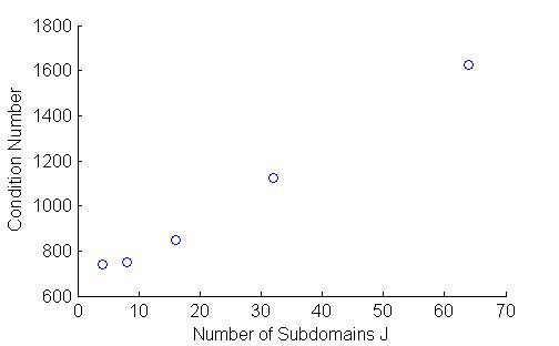
(a) Plot of J vs. $\kappa_{A}(P_{ad})$

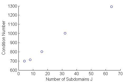
(b) Plot of J vs. $\kappa_{A}(P_{hy})$

Fig. 1: Dependence of $\kappa_{A}(P_{ad})$ and $\kappa_{A}(P_{hy})$ on J in Test 2

3. In all of these tests $\kappa_{A}(P_{ad})$ and $\kappa_{A}(P_{hy})$ depend on the number of subdomains $J$. Particularly in Test 2, we see an example that exhibits approximate linear dependence. See figure 1.

4. For $\|E_{mu}\|_{A}$ we do not observe such a strong dependence on the number of subdomains $J$.

5. In these tests $\|E_{mu}\|_{A}$ is greater than $1$; thus, we cannot rely upon this as an indicator for convergence of the multiplicative Schwarz iterative method.

6. $\kappa_{A}$ is not a unique metric in judging the convergence of GMRES after preconditioning with $P_{ad}$ and $P_{hy}$. For instance, in Test 4 $\kappa_{A}(P_{ad})$ decreases while the number of iterations necessary for GMRES increases as $J$ increases. This is opposite of the behavior that is observed in the previous tests.

Our numerical experiments verify that $\kappa_{A}$ is not a unique metric for the convergence of GMRES. Therefore, we must rely on other metrics to predict the convergence behavior of GMRES. The following theorem is used in [27] to test convergence of GMRES after Schwarz preconditioning in the indefinite case:

Theorem 18 ([13]).

Consider the linear system $A\mathbf{x}=\mathbf{b}$ where $A\in\mathbb{R}^{d\times d}$ and $\mathbf{x},\mathbf{b}\in\mathbb{R}^{d}$. If the symmetric part of $A$ is positive definite, then after $k$ step of GMRES, the norm of the residual $\mathbf{r_{k}}:=\mathbf{b}-A\mathbf{x}^{(k)}$ is bounded by

$$\|\mathbf{r_{k}}\|_{2}\leq\left(1-\frac{c_{p}^{2}}{C_{p}^{2}}\right)^{k/2}\|\mathbf{r_{0}}\|_{2},$$

where $c_{p}>0$ is the minimal eigenvalue of the symmetric part of $A$ and $C_{p}$ is the operator norm of $A$ given by

$$c_{p}:=\min_{\mathbf{u}\in\mathbb{R}^{d}}\frac{\langle\mathbf{u},A\mathbf{u}\rangle}{\langle\mathbf{u},\mathbf{u}\rangle},\qquad C_{p}:=\max_{\mathbf{u}\in\mathbb{R}^{d}}\frac{\|A\mathbf{u}\|_{2}}{\|\mathbf{u}\|_{2}}.$$

Unfortunately, this theorem cannot be applied in our case because we are not guaranteed that $P_{ad}$ and $P_{hy}$ have positive definite symmetric part (i.e., $c_{p}>0$). In the tests previously done, we find that these operators can be indefinite (i.e., $c_{p}<0$). Another result that could be of help in this area is the following theorem (cf. [28]).

Theorem 19.

Consider the linear system $A\mathbf{x}=\mathbf{b}$ where $A\in\mathbb{R}^{d\times d}$ and $\mathbf{x},\mathbf{b}\in\mathbb{R}^{d}$. Further suppose that $A$ is diagonalizable. Then after $k$ steps of GMRES, the residual $\mathbf{r}_{k}:=\mathbf{b}-A\mathbf{x}^{(k)}$ satisfies

$$\frac{\|\mathbf{r}_{k}\|_{2}}{\|\mathbf{b}\|_{2}}\leq\kappa_{2}(V)\inf_{\begin{subarray}{c}p\in\mathbb{P}_{k}\\ p(0)=1\end{subarray}}\sup_{\lambda\in\sigma(A)}|p(\lambda)|,$$

where $V$ is a nonsingular matrix of eigenvectors of $A$ and $\sigma(A)$ denotes the spectrum of $A$.

The above theorem says that the spread of the spectrum is a metric to judge the performance of GMRES with GMRES performing better when the spectrum of $A$ is clustered. With this theorem in mind, let us examine the spectrum of the matrix $A$ and $P_{ad}$ for $J=4,8,16,32,64$ obtained in Test 2 and Test 4.

Note that in Figure 2(a) and Figure 3(a) the spectrum has a large spread which is consistent with the fact that GMRES performed poorly on the original system without preconditioning. We also see that after preconditioning, the spectrum of $P_{ad}$ is clustered which corresponds to improved performance of GMRES after preconditioning with $P_{ad}$. Lastly, we note that as the number of subdomains $J$ increases, the spread of the spectrum of $P_{ad}$ increases. This corresponds to a decreased performance in GMRES after preconditioning with $P_{ad}$ as $J$ increases.

This result leads us to believe that to accurately judge the behavior of GMRES after preconditioning one needs to analyze the spectrum of the preconditioned system. Similarly, we find that to accurately predict the performance of the multiplicative Schwarz iterative method one needs to analyze the spectral radius of $E_{mu}$.

Another property of $\kappa_{A}(P_{ad})$ that is of interest is its dependence on the fine mesh parameter $h$ and the coarse mesh parameter $H$. It was shown in [14] that $\kappa_{A}(P_{ad})=O(\frac{H}{h})$ using two-level non-overlapping domain decomposition for an IPDG approximation of the equation (109) with $\mathbf{b}=0$ and $c=0$. This work uses the existing framework that is laid down for the symmetric and positive definite case. We would like to test our new framework to see if this dependence on $H$ and $h$ is still true. For this reason in Test 1 - 4 we have calculated $\kappa_{A}(P_{ad})$ with $1/h=16,32,64,128$ and $1/H=4,8,16$ when $J=4$. We also calculated $\kappa_{A}(P_{ad})$ with $1/h=32,64,128,256$ and $1/H=8,16,32$ when $J=8$. From Table 5 and Table 6 it seems that we cannot expect $\kappa_{A}(P_{ad})=O(\frac{H}{h})$ but instead we might expect the dependence to be one of the type

$$\kappa_{A}(P_{ad})=O\left(\frac{H^{\sigma_{1}}}{h^{\sigma_{2}}}\right)$$

where $\sigma_{1}$ and $\sigma_{2}$ are positive real numbers with $\sigma_{1}<\sigma_{2}$ or some other more complicated dependence on $H$ and $h$.

J	Iteration #		CPU Time		$\kappa_{A}$
	of GMRES
NA	552		14.3760		$3.3893\times 10^{4}$
	$P_{ad}$	$P_{hy}$	$P_{ad}$	$P_{hy}$	$P_{ad}$	$P_{hy}$
4	7	2	1.3638	1.1922	460.5713	397.3567
8	7	3	1.3343	1.2367	436.7967	398.2544
16	11	5	1.6873	1.4040	438.2207	412.1700
32	17	8	2.6431	1.9066	521.3530	478.9537
64	30	15	6.2315	3.7889	774.7091	619.3973

(a) GMRES after preconditioning with $P_{ad}$ and $P_{hy}$

J	Iterations # of	CPU Time	$\|E_{mu}\|_{A}$	$\rho(E_{mu})$
	Mult. Schwartz
4	2	1.1060	19.8830	$4.4793\times 10^{-6}$
8	2	1.1016	19.8889	0.0029
16	3	1.1352	19.8469	0.0725
32	5	1.2768	19.7658	0.3179
64	8	1.7129	19.7176	0.5926

(b) Multiplicative Schwarz Iteration

Table 1: Performance of three Schwarz methods on Test 1

J	Iteration #		CPU Time		$\kappa_{A}$
	of GMRES
NA	550		14.4971		$1.7388\times 10^{4}$
	$P_{ad}$	$P_{hy}$	$P_{ad}$	$P_{hy}$	$P_{ad}$	$P_{hy}$
4	8	3	1.3249	1.2069	741.9511	699.5729
8	10	5	1.4463	1.2835	749.0976	713.3674
16	17	8	1.9924	1.5557	847.4815	800.9121
32	27	14	5.5602	2.4255	$1.1221\times 10^{3}$	$1.0029\times 10^{3}$
64	44	24	8.7063	5.3089	$1.6247\times 10^{3}$	$1.2918\times 10^{3}$

(a) GMRES after preconditioning with $P_{ad}$ and $P_{hy}$

J	Iterations # of	CPU Time	$\|E_{mu}\|_{A}$	$\rho(E_{mu})$
	Mult. Schwartz
4	2	1.1010	26.4005	0.0011
8	3	1.1131	26.3187	0.0451
16	4	1.1679	26.1222	0.2529
32	6	1.3214	25.9832	0.5277
64	10	1.8713	25.9270	0.7167

(b) Multiplicative Schwarz Iteration

Table 2: Performance of three Schwarz methods on Test 2

J	Iteration #		CPU Time		$\kappa_{A}$
	of GMRES
NA	554		14.3919		$4.0782\times 10^{3}$
	$P_{ad}$	$P_{hy}$	$P_{ad}$	$P_{hy}$	$P_{ad}$	$P_{hy}$
4	8	3	1.3422	1.1772	647.6787	615.1005
8	12	5	1.4953	1.2517	658.7462	627.0064
16	18	9	2.0216	1.5588	726.3005	690.1682
32	27	15	3.5402	2.4623	854.1450	788.5277
64	35	23	7.1266	4.9327	939.5190	816.1892

(a) GMRES after preconditioning with $P_{ad}$ and $P_{hy}$

J	Iteration # of	CPU Time	$\|E_{mu}\|_{A}$	$\rho(E_{mu})$
	Mult. Schwartz
4	2	1.1067	24.7399	0.0021
8	2	1.0982	24.6200	0.0526
16	3	1.1394	24.4247	0.2350
32	5	1.2778	24.2986	0.4369
64	7	1.6321	24.2524	0.5302

(b) Multiplicative Schwarz Iteration

Table 3: Performance of three Schwarz methods on Test 3

J	Iteration #		CPU Time		$\kappa_{A}$
	of GMRES
NA	468		9.4276		$1.0769\times 10^{3}$
	$P_{ad}$	$P_{hy}$	$P_{ad}$	$P_{hy}$	$P_{ad}$	$P_{hy}$
4	8	2	1.3305	1.2039	103.5739	31.7538
8	11	2	1.4551	1.2558	75.7527	31.6954
16	14	3	1.8217	1.3019	56.6486	31.6803
32	13	5	2.2940	1.6227	46.4141	31.8710
64	15	8	3.7025	2.5950	44.1292	32.2846

(a) GMRES after preconditioning with $P_{ad}$ and $P_{hy}$

J	Iteration # of	CPU Time	$\|E_{mu}\|_{A}$	$\rho(E_{mu})$
	Mult. Schwartz
4	2	1.0996	5.4574	$85394\times 10^{-9}$
8	2	1.0984	5.4575	$1.0873\times 10^{-6}$
16	2	1.1157	5.4575	$6.6472\times 10^{-4}$
32	2	1.1566	5.4560	0.0158
64	2	1.2399	5.4540	0.0678

(b) Multiplicative Schwarz Iteration

Table 4: Performance of three Schwarz methods on Test 4

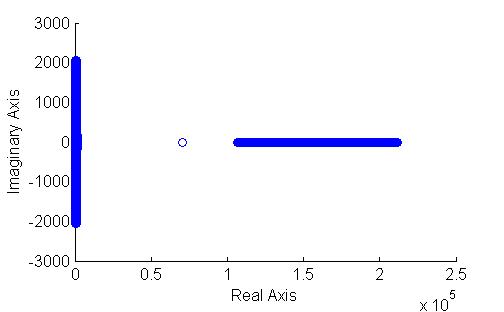
(a) Plot of $\sigma(A)$

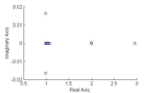
(b) Plot of $\sigma(P_{ad})$ with J = 4

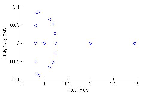
(c) Plot of $\sigma(P_{ad})$ with J = 8

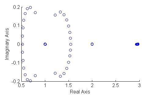
(d) Plot of $\sigma(P_{ad})$ with J = 16

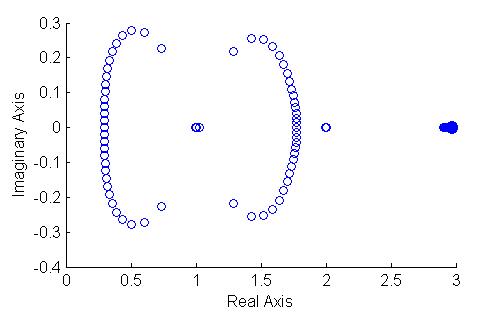
(e) Plot of $\sigma(P_{ad})$ with J = 32

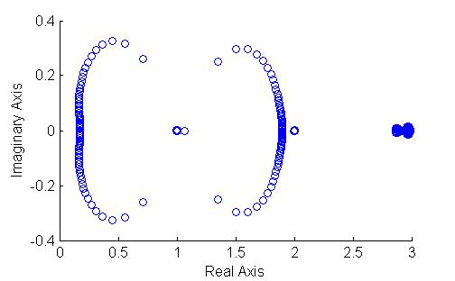
(f) Plot of $\sigma(P_{ad})$ with J = 64

Fig. 2: Spectrum plots from Test 2

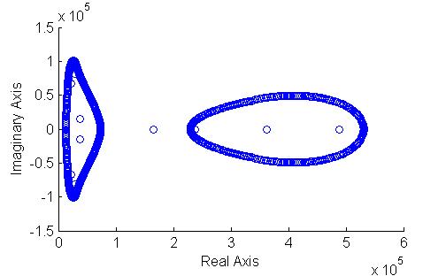
(a) Plot of $\sigma(A)$

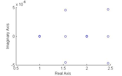
(b) Plot of $\sigma(P_{ad})$ with J = 4

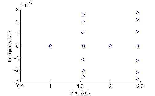
(c) Plot of $\sigma(P_{ad})$ with J = 8

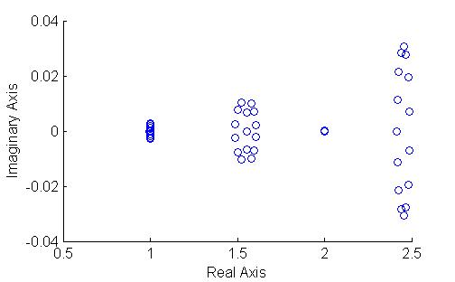
(d) Plot of $\sigma(P_{ad})$ with J = 16

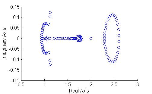
(e) Plot of $\sigma(P_{ad})$ with J = 32

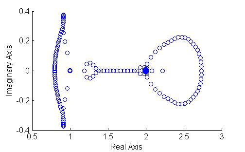
(f) Plot of $\sigma(P_{ad})$ with J = 64

Fig. 3: Spectrum plots from Test 4

	16	32	64	128
4	65.7321	421.0708	$2.6132\times 10^{3}$	$1.5015\times 10^{4}$
8	31.1342	182.6298	$1.0812\times 10^{3}$	$5.2251\times 10^{3}$
16	9.1835	66.5400	325.8230	$1.3700\times 10^{3}$

(a) Test 1

	16	32	64	128
4	29.9211	167.5776	$1.0288\times 10^{3}$	$6.5720\times 10^{3}$
8	16.9208	87.8272	567.0238	$3.4546\times 10^{3}$
16	7.9795	43.6354	249.6884	$1.4125\times 10^{3}$

(b) Test 2

	16	32	64	128
4	9.8123	28.7663	120.0237	598.6388
8	8.1720	18.9775	77.8493	413.6956
16	7.0895	15.4453	52.6716	279.7399

(c) Test 3

	16	32	64	128
4	7.7226	13.6618	27.8054	68.6090
8	7.2057	12.2264	23.0226	50.6394
16	6.9673	11.7750	21.6517	45.9328

(d) Test 4

Table 5: Behavior of $\kappa_{A}(P_{ad})$ as $h$ and $H$ vary when $J=4$.

	32	64	128	256
8	212.7543	$1.3522\times 10^{3}$	$6.7950\times 10^{3}$	$2.7336\times 10^{4}$
16	75.7638	428.5503	$1.8990\times 10^{3}$	$6.2384\times 10^{3}$
32	11.0954	108.7492	441.1266	$1.4728\times 10^{3}$

(a) Test 1

	32	64	128	256
8	98.1017	669.2190	$4.1498\times 10^{3}$	$2.3439\times 10^{4}$
16	45.5532	306.0990	$1.8395\times 10^{3}$	$8.5735\times 10^{3}$
32	9.3610	111.3056	605.5322	$2.6167\times 10^{3}$

(b) Test 2

	32	64	128	256
8	17.5492	84.0599	470.5346	$2.7253\times 10^{3}$
16	12.2180	50.0108	314.2682	$1.9264\times 10^{3}$
32	8.2829	31.6447	183.8996	$1.2169\times 10^{3}$

(c) Test 3

	32	64	128	256
8	9.0739	16.7773	42.5919	147.1763
16	8.6294	15.0583	32.3845	107.8848
32	8.3903	14.4013	29.2256	91.4682

(d) Test 4

Table 6: Behavior of $\kappa_{A}(P_{ad})$ as $h$ and $H$ vary when $J=8$.

Acknowledgment: This work was initiated while the first autthor was a long term visitor of the IMA at University of Minnesota in Fall 2010. The first author would like to thank the IMA for its financial support and its hospitality. The first author would also like to thank Blanca Ayuso and Ohannes Karakashian for their many stimulating and critical discussions which have substantially helped to shape the structure and results of this paper.

References

- [1] B. Ayuso and L. D. Marini, Discontinuous Galerkin methods for advection-diffusion-reaction problems, SIAM J. Numer. Anal. (47), 2009, pp. 1391–1420.
- [2] P. F. Antonietti and B. Ayuso, Schwarz domain decomposition preconditioners for discontinuous Galerkin approximations of elliptic problems: non-overlapping case, M2AN Math. Model. Numer. Anal., (41), 2007, pp. 21–54.
- [3] I. Babuška, Error bound for the finite element method, Numer. Math., (16), 1971, pp. 322–333.
- [4] I. Babuška and A. K. Aziz, Survey lectures on the mathematical foundations of finite element method, A.K. Aziz (ed.), The Mathematical Foundations of the FEM with Application to PDE, Academic Press, 1972, pp. 5–359.
- [5] C. Bernardi and Y. Maday, Spectral methods, In Handbook of numerical analysis, Vol. V, Handb. Numer. Anal., V, pages 209–485. North-Holland, Amsterdam, 1997.
- [6] J. H. Bramble, J. E. Pasciak, J Wang and J Xu, Convergence estimates for product iterative methods with applications to domain decomposition, Math. Comp., (57), 1991, pp. 1–21.
- [7] S. C. Brenner and L. R. Scott, The Mathematical Theory of Finite Element Methods, 3rd Edition, Springer, New York, 2008.
- [8] F. Brezzi, On the existence uniqueness and approximation of saddle-point problems arising from Lagrange multipliers, RAIRO, R.2, 1974, pp. 129–151.
- [9] F. Brezzi and M. Fortin, Mixed and Hybrid Finite Element Method, Springer, New York, 1991
- [10] X.-C. Cai and O. B. Widlund, “Domain decomposition algorithms for indefinite elliptic problems”, SIAM J. Sci. Statist. Comput., (13), 1992, pp. 243–258.
- [11] P. G. Ciarlet, The Finite Element Method for Elliptic Problems. North-Holland, Amsterdam, 1978.
- [12] M. Dryja and O. B. Widlund, Towards a unified theory of domain decomposition algorithms for elliptic problems, Proceedings of Third International Symposium on Domain Decomposition Methods for Partial Differential Equations (T. Chan etc. editors), SIAM, Philadelphia, 1990. pp. 3–21.
- [13] S. C. Eisenstat, H. C. Elman, and M. H. Schultz, Variational iterative methods for nonsymmetric systems of linear equations, SIAM J. Numer. Anal. (20)2,1983, pp. 345 - 357.
- [14] X. Feng and O. A. Karakashian, Two-level additive Schwarz methods for a discontinuous Galerkin approximation of second order elliptic problems, SIAM J. Numer. Anal. (39)39, 2001, pp. 1343–1365.
- [15] X. Feng and O. A. Karakashian, Two-level non-overlapping Schwarz preconditioners for a discontinuous Galerkin approximation of the biharmonic equation, J. Sci. Comput. (22/23), 2005, pp. 289–314.
- [16] D. Gilbarg, N.S. Trudinger, Elliptic Partial Differential Equations of Second Order, Second Edition, Springer, New York, 2000.
- [17] G. H. Golub and C. F. Van Loan, Matrix Computation, 3rd Edition, Johns Hopkins University Press, 1996.
- [18] P. Houston, E. Süli and C. Schwab, Discontinuous -finite element methods for advection-diffusion-reaction problems, SIAM J. Numer. Anal., (39), 2002, pp. 2133–2163.
- [19] P. D. Lax and A. N. Milgram, Parabolic equations, Ann. Math. Studies, (33), 1954, pp. 167–190.
- [20] C. Lasser and A. Toselli, An overlapping domain decomposition preconditioner for a class of discontinuous Galerkin approximations of advection-diffusion problems, Math. Comp., (72), 2003, pp. 1215–1238.
- [21] L. Nirenberg, Remarks on strongly elliptic partial differential equations, Comm. Pure Appl. Math., (8), 1955, pp. 648–674.
- [22] A. Quarteroni and A. Valli, Domain Decomposition Methods for Partial Differential Equations, Oxford University Press, New York, 1999
- [23] B. Rivière, Discontinuous Galerkin Methods for Solving Elliptic and Parabolic Equations. SIAM, Philadelphia, PA, 2008.
- [24] I. Rosca, On the Babuška Lax Milgram theorem, An. Univ. Bucuresti, XXXVIII, (3)1989, pp. 61–65.
- [25] B. E. Smith, P. E. Bjørstad and W. D. Gropp, Domain Decomposition, Parallel Multilevel Methods for Elliptic Partial Differential Equations. Cambridge University Press, New York, 1996.
- [26] H. A. Schwarz, Über einen Grenzübergang durch alternierendes Verfahren, Vierteljahrsschrift der Naturforschenden Gesellschaft in Zürich, (15), 1870, pp. 272–286.
- [27] A. Toselli and O. Widlund, Domain Decomposition Methods - Algorithms and Theory, Springer, 2005.
- [28] L. Trefethen, D. Bau, Numerical Linear Algebra, Siam, 1997.
- [29] J. Xu, Iterative methods by space decomposition and subspace correction. SIAM Review, (34), 1992, pp. 581–613.
- [30] J. Xu and L. Zikatanov, The method of alternating projections and the method of subspace corrections in Hilbert space, J. Amer. Math. Soc., (15), 2002, pp. 573–597.