Confidence Sets Based on Thresholding Estimators in High-Dimensional Gaussian Regression Models

Abstract

We study confidence intervals based on hard-thresholding, soft-thresholding, and adaptive soft-thresholding in a linear regression model where the number of regressors $k$ may depend on and diverge with sample size $n$. In addition to the case of known error variance, we define and study versions of the estimators when the error variance is unknown. In the known-variance case, we provide an exact analysis of the coverage properties of such intervals in finite samples. We show that these intervals are always larger than the standard interval based on the least-squares estimator. Asymptotically, the intervals based on the thresholding estimators are larger even by an order of magnitude when the estimators are tuned to perform consistent variable selection. For the unknown-variance case, we provide non-trivial lower bounds and a small numerical study for the coverage probabilities in finite samples. We also conduct an asymptotic analysis where the results from the known-variance case can be shown to carry over asymptotically if the number of degrees of freedom $n-k$ tends to infinity fast enough in relation to the thresholding parameter.

1 Introduction

We study confidence sets based on thresholding estimators such as hard-thresholding, soft-thresholding, and adaptive soft-thresholding in a Gaussian linear regression model when the number of regressors can be large. When the regressors are orthogonal, the estimators we consider can be viewed as penalized least-squares estimators, with soft-thresholding then coinciding with the Lasso (introduced by Frank & Friedman, 1993, Alliney & Ruzinsky, 1994, and Tibshirani, 1996) and adaptive soft-thresholding coinciding with the adaptive Lasso (introduced by Zou, 2006). Thresholding estimators have of course been discussed earlier in the context of model selection (see Bauer et al., 1988) and in the context of wavelets (see, e.g. Donoho et al., 1995).

These types of estimators also widely gained importance in the context of econometric models: Belloni & Chernozhukov (2011) provide a discussion of using Lasso-type estimators in econometrics, including applications to earning regressions, instrument selection, and cross-country growth regressions. Caner & Knight (2013) introduce Bridge estimators (of which the Lasso is a special case) to the to the framework of unit root tests, whereas Caner & Zhang (2014) investigate the elastic net estimator (merging the Lasso with ridge regression) in the context of generalized method of moments estimators. For using thresholding estimators in connection with econometric models, see e.g. Bai & Ng (2008) who use hard- and soft-thresholding for factor forecasting.

When using and applying these kinds of estimators to econometric (and other) models, it is of course of importance to know about the statistical performance of the estimator in question, in particular of how to perform valid inference (see also Berk et al. (2013) for a treatment within a different context). For this, knowledge of the distributional properties of the particular estimator is needed. Contributions concerning such properties of thresholding and penalized least-squares estimators include the following: Knight & Fu (2000) derive the asymptotic distribution of the Lasso and related estimators when they are tuned to act as a conservative variable selection procedure, while the asymptotic distribution of the Lasso and the adaptive Lasso estimator when tuned as a consistent variable selection procedure is considered in Zou (2006). The asymptotic distribution of the so-called smoothly clipped absolute deviation (SCAD) estimator is derived in Fan & Li (2001) and Fan & Peng (2004) also under consistent tuning. Following this work, many papers have been published that study the asymptotic distribution of various penalized least-squares estimators when those are tuned to act as a consistent variable selection procedure, see the introduction in Pötscher & Schneider (2009) for a partial list. With the exception of Knight & Fu (2000), all these papers consider a so-called fixed-parameter framework for the asymptotic results. But as pointed out in Leeb & Pötscher (2005), such a framework may be highly misleading in the context of variable selection procedures and penalized least-squares estimators. To this end, Pötscher & Leeb (2009) and Pötscher & Schneider (2009) carry out a detailed study of the finite-sample as well as large-sample distribution of various penalized least-squares estimators, adopting a moving-parameter framework for the asymptotic results. While these two papers are set in the framework of an orthogonal linear regression model with a fixed number of parameters and known error variance, Pötscher & Schneider (2011) investigate finite-sample and large-sample distributions for thresholding estimators also for non-orthogonal regressors and a potentially diverging number of parameters.

Given all these distributional results in finite samples as well as asymptotically within a moving parameter framework, a natural question is of course what these results imply for confidence sets, as this is an important issue for statistical inference. To address this question, Pötscher & Schneider (2010) consider confidence intervals based on hard-thresholding, Lasso, and adaptive Lasso within an orthogonal linear regression model with normal errors. In the present paper, we extend these results relaxing the condition of orthogonality as well as allowing for a high-dimensional framework where the number of parameters $k$ may depend on and diverge with sample size $n$. The estimators we consider are hard-, soft-, and adaptive soft-thresholding acting componentwise. In addition to the case of known error variance $\sigma^{2}$, we define versions of the estimators when the error variance is unknown. We also make use of some distributional results derived in Pötscher & Schneider (2011).

Our main contributions and findings are as follows. In the case of known error variance, we derive explicit expressions for the minimal coverage probabilities of fixed (non-random) width confidence intervals in finite samples based on the estimators in question. We show that symmetric intervals are the shortest. The interval based on soft-thresholding is smaller than the one based on adaptive soft-thresholding which in turn is smaller than the one based on hard-thresholding. Compared to the standard interval based on the least-squares estimator, the intervals based on the thresholding estimators are all larger in finite samples. Asymptotically, two different pictures arise: when the estimators are tuned to perform conservative model selection, the lengths of the intervals are all of the same order which essentially is $n^{-1/2}$. If the estimators are tuned to carry out consistent selection, however, it turns out the lengths of the intervals based on the thresholding estimators are larger by an order of magnitude compared to the standard one based on least-squares estimation.

In the case of unknown error variance, we consider symmetric intervals of random width (where the randomness is introduced by scaling the length with an estimate of the error standard deviation). We provide lower and upper bounds for the minimal coverage probabilities of the intervals based on the thresholding estimators under consideration. When comparing the lengths of the intervals based on the thresholding estimators to the standard one based on least-squares estimation, asymptotically we arrive at the same conclusions as in the known-variance case. We also find that the effect of having to estimate the error variance disappears asymptotically only the number of degrees of freedom $n-k$ diverges fast enough in relation to the tuning (thresholding) parameter of the estimators.

The paper is organized as follows. We introduce the model and define the estimators and some notation in Section 2. Sections 3 and 4 derive auxiliary results for the finite- and large sample distributions of the thresholding estimators which are needed later for the study of confidence intervals in the main Section 5. Section 6 contains a short summary, and a table with an overview of assumptions and results is given in Appendix A. Finally, proofs are relegated to Appendix B.

2 The Model and the Estimators

Assumption M.

The model we consider is the linear regression model

$$y=X\theta+u,$$

where $y$ is the $n\times 1$ data vector, $X$ is a non-stochastic $n\times k$ matrix of rank $k\geq 1$ containing the regressors, and $u\sim N(0,\sigma^{2}I_{n})$.

We allow $k$, the number of columns of $X$, as well as the entries of $y$, $X$, and $u$ to depend on sample size $n$, although we almost always suppress this dependence on $n$ in the notation. Note that this framework allows for high-dimensional regression models, where the number of regressors $k$ may diverge, as well as for the more classical situation where $k$ remains fixed. Let

$$\hat{\theta}_{LS} = \left(X^{\prime}X\right)^{-1}X^{\prime}y$$

$$\hat{\sigma}^{2} = (y-X\hat{\theta}_{LS})^{\prime}(y-X\hat{\theta}_{LS})/(n-k)$$

denote the least-squares estimator for $\theta$ and the associated estimator for $\sigma^{2}$, the latter being defined only if $n>k$. Furthermore, we denote by $\xi_{i,n}$ the non-negative square root of $((X^{\prime}X/n)^{-1})_{ii}$, the $i$-th diagonal element of $(X^{\prime}X/n)^{-1}$. Note that in the textbook case where $k$ is fixed and $X^{\prime}X/n$ is assumed to converge to a finite positive definite matrix, $\xi_{i,n}$ asymptotically settles at a finite value greater than zero.

Definition 1.

The hard-thresholding estimator $\tilde{\theta}_{H}=(\tilde{\theta}_{H,1},\dots,\tilde{\theta}_{H,k})^{\prime}$ is defined via its components as follows

$$\tilde{\theta}_{H,i}=\tilde{\theta}_{H,i}(\eta_{i,n})=\hat{\theta}_{LS,i}\,\boldsymbol{1}\left(\left|\hat{\theta}_{LS,i}\right|>\hat{\sigma}\xi_{i,n}\eta_{i,n}\right),$$

where the tuning or thresholding parameters $\eta_{i,n}$ are positive real numbers that may change over components and $\hat{\theta}_{LS,i}$ denotes the $i$-th component of the least-squares estimator. We also consider its infeasible counterpart $\hat{\theta}_{H}=(\hat{\theta}_{H,i},\dots,\hat{\theta}_{H,i})$ given by

$$\hat{\theta}_{H,i}=\hat{\theta}_{H,i}(\eta_{i,n})=\hat{\theta}_{LS,i}\,\boldsymbol{1}\left(\left|\hat{\theta}_{LS,i}\right|>\sigma\xi_{i,n}\eta_{i,n}\right),$$

assuming knowledge of the error variance $\sigma^{2}$. The soft-thresholding estimator $\tilde{\theta}_{S}$ and its infeasible counterpart $\hat{\theta}_{S}$ are given by the components

$$\tilde{\theta}_{S,i} = \tilde{\theta}_{S,i}(\eta_{i,n})\;=\;\operatorname{sgn}(\hat{\theta}_{LS,i})\left(\left|\hat{\theta}_{LS,i}\right|-\hat{\sigma}\xi_{i,n}\eta_{i,n}\right)_{+}$$

$$= \left\{\begin{array}[]{cc}0&\text{ if }|\hat{\theta}_{LS,i}|\leq\hat{\sigma}\xi_{i,n}\eta_{i,n}\\ \hat{\theta}_{LS,i}-\operatorname{sgn}(\hat{\theta}_{LS,i})\hat{\sigma}\xi_{i,n}\eta_{i,n}&\text{ if }|\hat{\theta}_{LS,i}|>\hat{\sigma}\xi_{i,n}\eta_{i,n}\end{array}\right.$$

and

$$\hat{\theta}_{S,i} = \hat{\theta}_{S,i}(\eta_{i,n})\;=\;\operatorname{sgn}(\hat{\theta}_{LS,i})\left(\left|\hat{\theta}_{LS,i}\right|-\sigma\xi_{i,n}\eta_{i,n}\right)_{+}$$

$$= \left\{\begin{array}[]{cc}0&\text{ if }|\hat{\theta}_{LS,i}|\leq\sigma\xi_{i,n}\eta_{i,n}\\ \hat{\theta}_{LS,i}-\operatorname{sgn}(\hat{\theta}_{LS,i})\sigma\xi_{i,n}\eta_{i,n}&\text{ if }|\hat{\theta}_{LS,i}|>\sigma\xi_{i,n}\eta_{i,n},\end{array}\right.$$

where $(\cdot)_{+}=\max(\cdot,0)$. Finally, the adaptive soft-thresholding estimator $\tilde{\theta}_{AS}$ and its infeasible counterpart $\hat{\theta}_{AS}$ are defined componentwise via

$$\tilde{\theta}_{AS,i} = \tilde{\theta}_{AS,i}(\eta_{i,n})\;=\;\hat{\theta}_{LS,i}\left(1-\hat{\sigma}^{2}\xi_{i,n}^{2}\eta_{i,n}^{2}/\hat{\theta}_{LS,i}^{2}\right)_{+}$$

$$= \left\{\begin{array}[]{cc}0&\text{ if }|\hat{\theta}_{LS,i}|\leq\hat{\sigma}\xi_{i,n}\eta_{i,n}\\ \hat{\theta}_{LS,i}-\hat{\sigma}^{2}\xi_{i,n}^{2}\eta_{i,n}^{2}/\hat{\theta}_{LS,i}&\text{ if }|\hat{\theta}_{LS,i}|>\hat{\sigma}\xi_{i,n}\eta_{i,n}\end{array}\right.$$

and

$$\hat{\theta}_{AS,i} = \hat{\theta}_{AS,i}(\eta_{i,n})\;=\;\hat{\theta}_{LS,i}\left(1-\sigma^{2}\xi_{i,n}^{2}\eta_{i,n}^{2}/\hat{\theta}_{LS,i}^{2}\right)_{+}$$

$$= \left\{\begin{array}[]{cc}0&\text{ if }|\hat{\theta}_{LS,i}|\leq\sigma\xi_{i,n}\eta_{i,n}\\ \hat{\theta}_{LS,i}-\sigma^{2}\xi_{i,n}^{2}\eta_{i,n}^{2}/\hat{\theta}_{LS,i}&\text{ if }|\hat{\theta}_{LS,i}|>\sigma\xi_{i,n}\eta_{i,n}.\end{array}\right.$$

Note that $\tilde{\theta}_{H}$, $\tilde{\theta}_{S}$, and $\tilde{\theta}_{AS}$ as well as their infeasible counterparts are equivariant under scaling of the columns of $(y:X)$ by non-zero column-specific scale factors. We have chosen to let the thresholds $\hat{\sigma}\xi_{i,n}\eta_{i,n}$ ($\sigma\xi_{i,n}\eta_{i,n}$, respectively) depend explicitly on $\hat{\sigma}$ ($\sigma$, respectively) and $\xi_{i,n}$ in order to give $\eta_{i,n}$ an interpretation independent of the values of $\sigma$ and $X$. Often $\eta_{i,n}$ will be chosen independently of $i$, i.e., $\eta_{i,n}=\eta_{n}$ where $\eta_{n}$ is a positive real number. Clearly, for the feasible versions we always need to assume $n>k$, whereas for the infeasible versions $n\geq k$ suffices.

Aside from requiring that the regressor matrix $X$ has full column rank, we essentially have no assumptions on the regressor matrix $X$ except that for simplicity for all asymptotic considerations, we assume the following.

Assumption A.

Let $\xi_{i,n}^{2}/n=((X^{\prime}X)^{-1})_{i,i}$ satisfy

$$\sup_{n}\xi_{i,n}^{2}/n<\infty$$

for every fixed $i\geq 1$ satisfying $i\leq k(n)$ for large enough $n$.

Note that Assumption A is not really restrictive in the sense that the case excluded by it implies unboundedness of $\xi_{i,n}^{2}/n$, which in particular would entail inconsistency of the least-squares estimator.

We now turn to some definitions in terms of the asymptotic regimes we consider. Clearly, all three estimators exhibit positive probability of being set equal to 0 and in that sense they perform variable selection. Asymptotically, we will distinguish two different cases for this. Let $\breve{\theta}_{i}$ denote any of the thresholding estimators introduced above.

Definition 2.

The case of consistent variable selection occurs when

$$\lim_{n\to\infty}P_{n,\theta,\sigma}(\breve{\theta}_{i}=0)=1\;\;\text{ whenever }\theta_{i}=0,$$

in which we shall refer to $\breve{\theta}_{i}$ as being consistently tuned. The other case is the case of conservative variable selection where

$$\limsup_{n\to\infty}P_{n,\theta,\sigma}(\breve{\theta}_{i}=0)<1\;\;\text{ whenever }\theta_{i}=0,$$

in which we shall call $\breve{\theta}_{i}$ conservatively tuned.

Propositions 4 and 10 in Pötscher & Schneider (2011) show that $\breve{\theta}_{i}$ is consistently tuned when $n^{1/2}\eta_{i,n}\to\infty$, and conservatively tuned when $n^{1/2}\eta_{i,n}\to e_{i}$ with $0\leq e_{i}<\infty$, including the case $e_{i}=0$ in which $\breve{\theta}_{i}$ can be shown to be asymptotically equivalent to $\hat{\theta}_{LS,i}$ (see Remark 17 in the above reference). Moreover, Theorem 16 in the same reference shows that $\breve{\theta}_{i}$ is consistent for $\theta_{i}$ in terms of parameter estimation whenever $\xi_{i,n}\eta_{i,n}\to 0$ (in fact, the estimator is then even uniformly consistent) and this assumption will appear as a basic condition in all asymptotic considerations.

We conclude this section by introducing some more notation: $\hat{\theta}_{i}$ denotes any of the estimators $\hat{\theta}_{H,i}$, $\hat{\theta}_{S,i}$, or $\hat{\theta}_{AS,i}$ and $\tilde{\theta}_{i}$ any of the estimators $\tilde{\theta}_{H,i}$, $\tilde{\theta}_{S,i}$, or $\tilde{\theta}_{AS,i}$. Let $\overline{\mathbb{R}}$ be the extended real line $\mathbb{R}\cup\{-\infty,\infty\}$. Furthermore, $\Phi$ and $\phi$ are the cumulative distribution function (cdf) and the probability density function (pdf) of a standard normal distribution, respectively. By $T_{m}$ and $t_{m}$ we denote the cdf and pdf of a $t$-distribution with $m\in\mathbb{N}$ degrees of freedom, respectively. We use the convention $\Phi(\infty)=1$, $\Phi(-\infty)=0$ with a similar convention for $T_{m}$. By $\rho_{m}$ we denote the density function of $\sqrt{\chi^{2}_{m}/m}$, the square root of a chi-squared-distributed random variable divided by its degrees of freedom, $m$. For repeated later use, note that $T_{m}(x)=\int_{0}^{\infty}\Phi(xs)\rho_{m}(s)\,ds$. Finally, $\delta_{z}$ will denote the measure for pointmass at $z$.

3 Auxiliary Results: Finite-Sample Distributions

Pötscher & Schneider (2011) derive finite- and large-sample distributions of the thresholding estimators defined in Definition 1 for the case of known and of unknown error variance. More concretely, the finite-sample distributions of $\sigma^{-1}\alpha_{i,n}(\hat{\theta}_{i}-\theta_{i})$ and $\sigma^{-1}\alpha_{i,n}(\tilde{\theta}_{i}-\theta_{i})$ are derived, where $\alpha_{i,n}>0$ is a non-random scaling factor. When considering the large-sample distributions, the scaling factor $\alpha_{i,n}$ is set equal to $n^{1/2}/\xi_{i,n}$ in case of conservative tuning and equal to $(\xi_{i,n}\eta_{i,n})^{-1}$ in case of consistent tuning. These are shown to correspond to the uniform convergence rates of the estimators.

In the present paper, to analyze the coverage properties of confidence sets based on $\hat{\theta}_{i}$ in Section 5.1, we will make use of the finite-sample distributions of $\sigma^{-1}\alpha_{i,n}(\hat{\theta}_{i}-\theta_{i})$. These distributions were derived in in Propositions 19-21 Pötscher & Schneider (2011). In the unknown-variance case, to investigate the coverage probabilities of confidence sets based on $\tilde{\theta}_{i}$ in Section 5.2, we will need knowledge of the distributions of $\hat{\sigma}^{-1}\alpha_{i,n}(\tilde{\theta}_{i}-\theta_{i})$ with random scaling by $\hat{\sigma}^{-1}$ rather than the distributions of $\sigma^{-1}\alpha_{i,n}(\tilde{\theta}_{i}-\theta_{i})$ with non-random scaling which have been considered in the above mentioned paper.

To this end, we derive the finite-sample distributions of $\hat{\sigma}^{-1}\alpha_{i,n}(\tilde{\theta}_{i}-\theta_{i})$ in the following propositions and make some qualitative comparisons to the distributions of $\sigma^{-1}\alpha_{i,n}(\tilde{\theta}_{i}-\theta_{i})$. The corresponding large-sample distributions are considered in Section 4.

We shall suppress the dependence of the distribution function on the scaling factor $\alpha_{i,n}$ in the notation. Moreover, note that the distribution functions depend on the parameter $\theta$ only through the $i$-th component $\theta_{i}$. We start by considering the hard-thresholding estimator.

Proposition 3 (Hard-thresholding in finite samples).

The cdf $\tilde{H}^{i}_{H,n,\theta,\sigma}:=\tilde{H}^{i}_{H,\eta_{i,n},n,\theta,\sigma}$ of $\hat{\sigma}^{-1}\alpha_{i,n}(\tilde{\theta}_{H,i}-\theta_{i})$ is given by

$$\begin{split}&\tilde{H}^{i}_{H,n,\theta,\sigma}(x)\;=\;\int_{0}^{\infty}\left[\Phi\big{(}n^{1/2}xs/(\alpha_{i,n}\xi_{i,n})\big{)}\boldsymbol{1}\left(|xs/\alpha_{i,n}+\theta_{i}/\sigma|>\xi_{i,n}s\eta_{i,n}\right)\right.\\ &+\;\Phi\big{(}n^{1/2}(-\theta_{i}/(\sigma\xi_{i,n})+s\eta_{i,n})\big{)}\boldsymbol{1}\left(0\leq xs/\alpha_{i,n}+\theta_{i}/\sigma\leq\xi_{i,n}s\eta_{i,n}\right)\\ &\left.+\;\Phi\big{(}n^{1/2}(-\theta_{i}/(\sigma\xi_{i,n})-s\eta_{i,n})\big{)}\boldsymbol{1}\left(-\xi_{i,n}s\eta_{i,n}\leq xs/\alpha_{i,n}+\theta_{i}/\sigma<0\right)\right]\rho_{n-k}(s)\,ds,\end{split}$$ (5)

or equivalently, its measure is given by

$$\begin{split}d&\tilde{H}^{i}_{H,n,\theta,\sigma}(x)=\int_{0}^{\infty}\left[\Phi\big{(}n^{1/2}s\eta_{i,n}\big{)}-\Phi\big{(}-n^{1/2}s\eta_{i,n}\big{)}\right]\rho_{n-k}(s)\,ds\,d\delta_{0}(x)\\ &+\boldsymbol{1}\left(|x|>\alpha_{i,n}\xi_{i,n}\eta_{i,n}\right)\int_{0}^{\infty}(n^{1/2}s/(\alpha_{i,n}\xi_{i,n}))\phi\big{(}n^{1/2}xs/(\alpha_{i,n}\xi_{i,n})\big{)}\rho_{n-k}(s)\,dsdx\end{split}$$ (6)

for $\theta_{i}=0$, and by

$$\begin{split}d&\tilde{H}^{i}_{H,n,\theta,\sigma}(x)=\;\boldsymbol{1}\{-\operatorname{sgn}(\theta_{i})\,x\geq 0\}\,\alpha_{i,n}|\theta_{i}|/(\sigma x^{2})\,\rho_{n-k}\left(-\alpha_{i,n}\theta_{i}/(\sigma x)\right)\\ &\times\left[\Phi\big{(}-(n^{1/2}\theta_{i}/(\sigma\xi_{i,n}))(1+\alpha_{i,n}\xi_{i,n}\eta_{i,n}/x)\big{)}-\Phi\big{(}-(n^{1/2}\theta_{i}/(\sigma\xi_{i,n}))(1-\alpha_{i,n}\xi_{i,n}\eta_{i,n}/x)\big{)}\right]\,dx\\ &+\int_{0}^{\infty}(n^{1/2}s/(\alpha_{i,n}\xi_{i,n}))\phi\big{(}n^{1/2}xs/(\alpha_{i,n}\xi_{i,n})\big{)}\boldsymbol{1}\left(|xs/\alpha_{i,n}+\theta_{i}/\sigma|>\xi_{i,n}s\eta_{i,n}\right)\rho_{n-k}(s)\,dsdx\end{split}$$ (7)

in case $\theta_{i}\neq 0$.

Figure 1: Hard-thresholding: Plots of $d\tilde{H}^{i}_{H,n,\theta,\sigma}$ for (a) $\theta_{i}=0$ and (b) $\theta_{i}=0.16$. Exemplarily, in both plots we set $n=40$, $k=35$, $\eta_{i,n}=0.05$, $\xi_{i,n}=1$, $\sigma^{2}=1$, $\alpha_{i,n}=n^{1/2}/\xi_{i,n}$. The dot in part (a) corresponds to the total mass of the atomic part.

We now look at the soft-thresholding estimator.

Proposition 4 (Soft-thresholding in finite samples).

The cdf $\tilde{H}^{i}_{S,n,\theta,\sigma}:=\tilde{H}^{i}_{S,\eta_{i,n},n,\theta,\sigma}$ of $\hat{\sigma}^{-1}\alpha_{i,n}(\tilde{\theta}_{S,i}-\theta_{i})$ is given by

$$\begin{split}&\tilde{H}^{i}_{S,n,\theta,\sigma}(x)\;=\;\int_{0}^{\infty}\left[\Phi\big{(}n^{1/2}(xs/(\alpha_{i,n}\xi_{i,n})+s\eta_{i,n})\big{)}\boldsymbol{1}\left(xs/\alpha_{i,n}+\theta_{i}/\sigma\geq 0\right)\right.\\ &+\;\left.\Phi\big{(}n^{1/2}(xs/(\alpha_{i,n}\xi_{i,n})-s\eta_{i,n})\big{)}\boldsymbol{1}\left(xs/\alpha_{i,n}+\theta_{i}/\sigma<0\right)\right]\rho_{n-k}(s)\,ds,\end{split}$$ (8)

or equivalently, its measure is given by

$$\begin{split}d&\tilde{H}^{i}_{S,n,\theta,\sigma}(x)=\int_{0}^{\infty}\left[\Phi\big{(}n^{1/2}s\eta_{i,n}\big{)}-\Phi\big{(}-n^{1/2}s\eta_{i,n}\big{)}\right]\rho_{n-k}(s)\,ds\,d\delta_{0}(x)\\ &+\int_{0}^{\infty}(n^{1/2}s/(\alpha_{i,n}\xi_{i,n}))\left[\phi\big{(}n^{1/2}(xs/(\alpha_{i,n}\xi_{i,n})+s\eta_{i,n})\big{)}\boldsymbol{1}\left(x>0\right)\right.\\ &+\left.\phi\big{(}n^{1/2}(xs/(\alpha_{i,n}\xi_{i,n})-s\eta_{i,n})\big{)}\boldsymbol{1}\left(x<0\right)\right]\rho_{n-k}(s)\,dsdx\end{split}$$ (9)

for $\theta_{i}=0$ and by

$$\begin{split}d&\tilde{H}^{i}_{S,n,\theta,\sigma}(x)=\;\boldsymbol{1}\{-\operatorname{sgn}(\theta_{i})\,x\geq 0\}\,\alpha_{i,n}|\theta_{i}|/(\sigma x^{2})\,\rho_{n-k}\left(-\alpha_{i,n}\theta_{i}/(\sigma x)\right)\\ &\times\left[\Phi\big{(}-(n^{1/2}\theta_{i}/(\sigma\xi_{i,n}))(1+\alpha_{i,n}\xi_{i,n}\eta_{i,n}/x)\big{)}-\Phi\big{(}-(n^{1/2}\theta_{i}/(\sigma\xi_{i,n}))(1-\alpha_{i,n}\xi_{i,n}\eta_{i,n}/x)\big{)}\right]\,dx\\ &+\int_{0}^{\infty}(n^{1/2}s/(\alpha_{i,n}\xi_{i,n}))\left[\phi\big{(}n^{1/2}(xs/(\alpha_{i,n}\xi_{i,n})+s\eta_{i,n})\big{)}\boldsymbol{1}\left(xs/\alpha_{i,n}+\theta_{i}/\sigma>0\right)\right.\\ &+\left.\phi\big{(}n^{1/2}(xs/(\alpha_{i,n}\xi_{i,n})-s\eta_{i,n})\big{)}\boldsymbol{1}\left(xs/\alpha_{i,n}+\theta_{i}/\sigma<0\right)\right]\rho_{n-k}(s)\,dsdx\end{split}$$ (10)

in case $\theta_{i}\neq 0$.

Figure 2: Soft-thresholding: Plots of $d\tilde{H}^{i}_{S,n,\theta,\sigma}$ for (a) $\theta_{i}=0$ and (b) $\theta_{i}=0.16$. Exemplarily, in both plots we set to $n=40$, $k=35$, $\eta_{i,n}=0.05$, $\xi_{i,n}=1$, $\sigma^{2}=1$, $\alpha_{i,n}=n^{1/2}/\xi_{i,n}$. The dot in part (a) corresponds to the total mass of the atomic part.

We next consider the adaptive soft-thresholding estimator.

Proposition 5 (Adaptive soft-thresholding in finite samples).

The cdf $\tilde{H}^{i}_{AS,n,\theta,\sigma}:=\tilde{H}^{i}_{AS,\eta_{i,n},n,\theta,\sigma}$ of $\hat{\sigma}^{-1}\alpha_{i,n}(\tilde{\theta}_{AS,i}-\theta_{i})$ is given by

$$\begin{split}\tilde{H}^{i}_{AS,n,\theta,\sigma}(x)\;=\;&\int_{0}^{\infty}\left[\Phi\big{(}z_{n,\theta,\sigma}^{(2)}(xs,s\eta_{i,n})\big{)}\boldsymbol{1}\left(xs/\alpha_{i,n}+\theta_{i}/\sigma\geq 0\right)\right.\\ &+\left.\Phi\big{(}z_{n,\theta,\sigma}^{(1)}(xs,s\eta_{i,n})\big{)}\boldsymbol{1}\left(xs/\alpha_{i,n}+\theta_{i}/\sigma<0\right)\right]\rho_{n-k}(s)\,ds,\end{split}$$ (11)

or equivalently, its measure is given by

$$\begin{split}d&\tilde{H}^{i}_{AS,n,\theta,\sigma}(x)=\int_{0}^{\infty}\left[\Phi\big{(}n^{1/2}s\eta_{i,n}\big{)}-\Phi\big{(}-n^{1/2}s\eta_{i,n}\big{)}\right]\rho_{n-k}(s)\,ds\,d\delta_{0}(x)\\ &+\int_{0}^{\infty}0.5(n^{1/2}s/(\alpha_{i,n}\xi_{i,n}))\left[\phi\big{(}z_{n,\theta,\sigma}^{(2)}(xs,s\eta_{i,n})\big{)}(1+t_{n,\theta,\sigma}(xs,s\eta_{i,n}))\boldsymbol{1}\left(x>0\right)\right.\\ &+\left.\phi\big{(}z_{n,\theta,\sigma}^{(1)}(xs,s\eta_{i,n})\big{)}(1-t_{n,\theta,\sigma}(xs,s\eta_{i,n}))\boldsymbol{1}\left(x<0\right)\right]\rho_{n-k}(ds)\,dx\end{split}$$ (12)

for $\theta_{i}=0$ and by

$$\begin{split}d&\tilde{H}^{i}_{AS,n,\theta,\sigma}(x)=\;\boldsymbol{1}\{-\operatorname{sgn}(\theta_{i})\,x\geq 0\}\,\alpha_{i,n}|\theta_{i}|/(\sigma x^{2})\,\rho_{n-k}\left(-\alpha_{i,n}\theta_{i}/(\sigma x)\right)\\ &\times\left[\Phi\big{(}-(n^{1/2}\theta_{i}/(\sigma\xi_{i,n}))(1+\alpha_{i,n}\xi_{i,n}\eta_{i,n}/x)\big{)}-\Phi\big{(}-(n^{1/2}\theta_{i}/(\sigma\xi_{i,n}))(1-\alpha_{i,n}\xi_{i,n}\eta_{i,n}/x)\big{)}\right]\,dx\\ &+\int_{0}^{\infty}0.5(n^{1/2}s/(\alpha_{i,n}\xi_{i,n}))\left[\phi\big{(}z_{n,\theta,\sigma}^{(2)}(xs,s\eta_{i,n})\big{)}(1+t_{n,\theta,\sigma}(xs,s\eta_{i,n}))\boldsymbol{1}\left(xs/\alpha_{i,n}+\theta_{i}/\sigma>0\right)\right.\\ &+\left.\phi\big{(}z_{n,\theta,\sigma}^{(1)}(xs,s\eta_{i,n})\big{)}(1-t_{n,\theta,\sigma}(xs,s\eta_{i,n}))\boldsymbol{1}\left(xs/\alpha_{i,n}+\theta_{i}/\sigma<0\right)\right]\rho_{n-k}(ds)\,dx\end{split}$$ (13)

for $\theta_{i}\neq 0$, where $z_{n,\theta,\sigma}^{(1)}(u,v)\leq z_{n,\theta,\sigma}^{(2)}(u,v)$ are defined by

$$0.5n^{1/2}(u/\alpha_{i,n}-\theta_{i}/\sigma)/\xi_{i,n}\pm n^{1/2}\sqrt{\left(0.5(u/\alpha_{i,n}+\theta_{i}/\sigma)/\xi_{i,n}\right)^{2}+v^{2}},$$

and $t_{n,\theta,\sigma}(u,v)=0.5\xi_{i,n}^{-1}\left(u/\alpha_{i,n}+\theta_{i}/\sigma\right)/\left((0.5\xi_{i,n}^{-1}\big{(}u/\alpha_{i,n}+\theta_{i}/\sigma)^{2}+v^{2}\right)^{1/2}$.

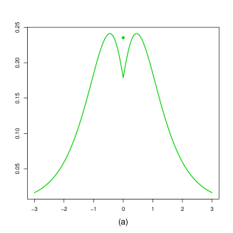
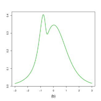
Figure 3: Adaptive Soft-thresholding: Plots of $d\tilde{H}^{i}_{AS,n,\theta,\sigma}$ for (a) $\theta_{i}=0$ and (b) $\theta_{i}=0.16$. Exemplarily, in both plots we set to $n=40$, $k=35$, $\eta_{i,n}=0.05$, $\xi_{i,n}=1$, $\sigma^{2}=1$, $\alpha_{i,n}=n^{1/2}/\xi_{i,n}$. The dot in part (a) corresponds to the total mass of the atomic part.

Propositions 3-5 show the following about the finite-sample distributions of $\hat{\sigma}^{-1}\alpha_{i,n}(\tilde{\theta}_{i}-\theta_{i})$. The distributions of all three estimators are non-normal and depend on the unknown parameter vector $\theta$ only through the $i$-th component $\theta_{i}$. In case $\theta_{i}=0$, they are made up of two components, one being pointmass at 0 and the other one being absolutely continuous (with respect to Lebesgue-measure) with a density that is generally bimodal. The pointmass part has the same weight for all three estimators and is represented by the first term in (6), (9), and (12) ending with $d\delta_{0}(x)$. The remaining second term, ending with $dx$, represents the absolutely continuous part. In case $\theta_{i}\neq 0$, the distributions are always absolutely continuous, as can be seen in in (7), (10), and (13).

Propositions 23-25 in Pötscher & Schneider (2011) show that the distributions of $\sigma^{-1}\alpha_{i,n}$ $\times(\tilde{\theta}_{i}-\theta_{i})$ with non-random scaling consist of pointmass and an absolutely continuous part for all values of $\theta_{i}$. This means that scaling the estimators by $\hat{\sigma}^{-1}$ instead of $\sigma^{-1}$ results in smoothing the distribution function to the extent that when $\theta_{i}\neq 0$, the previously existing pointmass is spread onto $\mathbb{R}_{-}$ or $\mathbb{R}_{+}$ in case $\theta_{i}>0$ or $\theta_{i}<0$, respectively, yielding a continuous distribution function for non-zero values of $\theta_{i}$. In case $\theta_{i}=0$, the atomic part of the distributions of $\sigma^{-1}\alpha_{i,n}(\tilde{\theta}_{i}-\theta_{i})$ remains the same as in the case of scaling by $\hat{\sigma}^{-1}$.

Curiously, on the other hand, scaling by $\hat{\sigma}^{-1}$ cancels out some smoothing effect of the unknown-variance hard-thresholding estimator $\hat{\theta}_{H,i}$ in case $\theta_{i}=0$: there, the density of the absolutely continuous part of the distribution is only piecewise continuous (has an excised part) both in the case of known variance and unknown variance with random $\hat{\sigma}^{-1}$-scaling, that is, for the distributions of $\sigma^{-1}\alpha_{i,n}(\hat{\theta}_{H,i}-\theta_{i})$ and $\hat{\sigma}^{-1}\alpha_{i,n}(\tilde{\theta}_{H,i}-\theta_{i})$, but not so for the case of unknown variance with non-random $\sigma^{-1}$-scaling, that is, for $\sigma^{-1}\alpha_{i,n}(\tilde{\theta}_{H,i}-\theta_{i})$, cf. Figure 1 in Pötscher & Leeb (2009) and the paragraph above Remark 26 in Pötscher & Schneider (2011).

4 Auxiliary Results: Large-Sample Distributions

We next derive the asymptotic distributions of $\hat{\sigma}^{-1}\alpha_{i,n}(\tilde{\theta}_{i}-\theta_{i})$ under a so-called moving-parameter framework where the unknown parameter $\theta$ is allowed to vary with sample size. It is well known that asymptotics based on a fixed-parameter framework only do not yield a representative picture of the finite-sample behavior and performance of the estimator, as is mentioned in the introduction in Section 1. In particular, we will need the asymptotic distributions of $\hat{\sigma}^{-1}\alpha_{i,n}(\tilde{\theta}_{i}-\theta_{i})$ under a moving-parameter framework in order to carry out a uniform analysis of the coverage properties of confidence intervals based on $\tilde{\theta}_{i}$ in Section 5.2.

The sequence of scaling factors $\alpha_{i,n}$ is chosen according to the uniform convergence rate of the estimators, that is, $\alpha_{i,n}=n^{1/2}/\xi_{i,n}$ in the case of conservative tuning, and $\alpha_{i,n}=(\xi_{i,n}\eta_{i,n})^{-1}$ in case of consistent tuning, see Theorem 16 in Pötscher & Schneider (2011).

Since the number of parameters $k$ may vary with sample size $n$, asymptotically, we distinguish the case where the number of degrees of freedom $n-k$ in the variance estimation tends to infinity, and the case where $n-k$ converges to a finite limit, implying that it eventually remains constant. For the case where $n-k\to\infty$, note that $\hat{\sigma}/\sigma$ converges to 1 in probability, so that the asymptotic distributions of $\hat{\sigma}^{-1}\alpha_{i,n}(\tilde{\theta}_{i}-\theta_{i})$ coincide with the asymptotic distributions of $\sigma^{-1}\alpha_{i,n}(\tilde{\theta}_{i}-\theta_{i})$ which have been derived in Pötscher & Schneider (2011).

Note that technically, for the proofs of Section 5, we make explicit use of the large-sample distributions in the consistently tuned case only. We state the distributions of the conservatively tuned case for completeness, but only list the case when $n-k$ converges to a finite limit. For the consistently tuned estimators, we also quote the case when $n-k\to\infty$ since the results are directly relevant for Section 5.

4.1 Conservative Tuning

We first consider the case where the estimators are tuned to perform conservative variable selection implying that the sequence of tuning parameters satisfies $n^{1/2}\eta_{i,n}\to e_{i}$ with $0\leq e_{i}<\infty$. We start by looking at the hard-thresholding estimator and derive the asymptotic distribution of $\hat{\sigma}^{-1}(n^{1/2}/\xi_{i,n})(\tilde{\theta}_{H,i}-\theta_{i})$.

Proposition 6 (Hard-thresholding with conservative tuning).

Suppose that for a given $i\geq 1$ satisfying $i\leq k=k(n)$ for large enough $n$ we have $\xi_{i,n}\eta_{i,n}\to 0$ and $n^{1/2}\eta_{i,n}\to e_{i}$ where $0\leq e_{i}<\infty$. Set the scaling factor $\alpha_{i,n}=n^{1/2}/\xi_{i,n}$. Suppose that the true parameters $\theta^{(n)}=(\theta_{1,n},\dots,\theta_{k_{n},n})\in\mathbb{R}^{k_{n}}$ and $\sigma_{n}\in(0,\infty)$ satisfy $n^{1/2}\theta_{i,n}/(\sigma_{n}\xi_{i,n})\to\nu_{i}\in\overline{\mathbb{R}}$ and that $n-k\to m$ in $\mathbb{N}$. Then $\tilde{H}^{i}_{H,n,\theta^{(n)},\sigma_{n}}$ converges weakly to the distribution with cdf

$$\begin{split}\int_{0}^{\infty}&\big{[}\Phi\left(xs\right)\boldsymbol{1}\left(|xs+\nu_{i}|>se_{i}\right)+\Phi\left(-\nu_{i}+se_{i}\right)\boldsymbol{1}\left(0\leq xs+\nu_{i}\leq se_{i}\right)\\ &+\Phi\left(-\nu_{i}-se_{i}\right)\boldsymbol{1}\left(-se_{i}\leq xs+\nu_{i}<0\right)\big{]}\rho_{m}(s)\,ds.\end{split}$$ (14)

The corresponding measure is given by

$$\bigg{\{}\boldsymbol{1}\{-\operatorname{sgn}(\nu_{i}) \,x\geq 0\}\,|\nu_{i}|/x^{2}\,\rho_{m}\left(-\nu_{i}/x\right)\big{[}\Phi\left(-\nu_{i}(1+e_{i}/x)\right)-\Phi\left(-\nu_{i}(1-e_{i}/x)\right)\big{]}$$

$$+\left.\int_{0}^{\infty}s\phi\left(xs\right)\boldsymbol{1}\left(|xs+\nu_{i}|>se_{i}\right)\rho_{m}(s)\,ds\right\}dx$$

for $0<|\nu_{i}|<\infty$ and by

$$\big{[}T_{m}(e_{i})-T_{m}(-e_{i})\big{]}d\delta_{0}(x)+\boldsymbol{1}\left(|x|>e_{i}\right)t_{m}(x)\,dx$$

for $\nu_{i}=0$.

Note that the limiting distribution in the above proposition is a $t$-distribution with $m$ degrees of freedom in case $|\nu_{i}|=\infty$ or $e_{i}=0$. Moreover, if $\nu_{i}=0$, the expression in (14) simplifies to

$$T_{m}(x)\boldsymbol{1}\left(|x|>e_{i}\right)+T_{m}\left(e_{i}\right)\boldsymbol{1}\left(0\leq x\leq e_{i}\right)+T_{m}\left(-e_{i}\right)\boldsymbol{1}\left(-e_{i}\leq x<0\right).$$

By the argument given above, the limiting distribution for the case when $n-k\to\infty$ is the same as in Theorem 33(b) in Pötscher & Schneider (2011).

We now look at the soft-thresholding estimator and derive the asymptotic distribution of $\hat{\sigma}^{-1}(n^{1/2}/\xi_{i,n})(\tilde{\theta}_{S,i}-\theta_{i})$.

Proposition 7 (Soft-thresholding with conservative tuning).

Suppose that for a given $i\geq 1$ satisfying $i\leq k=k(n)$ for large enough $n$ we have $\xi_{i,n}\eta_{i,n}\to 0$ and $n^{1/2}\eta_{i,n}\to e_{i}$ where $0\leq e_{i}<\infty$. Set the scaling factor $\alpha_{i,n}=n^{1/2}/\xi_{i,n}$. Suppose that the true parameters $\theta^{(n)}=(\theta_{1,n},\dots,\theta_{k_{n},n})\in\mathbb{R}^{k_{n}}$ and $\sigma_{n}\in(0,\infty)$ satisfy $n^{1/2}\theta_{i,n}/(\sigma_{n}\xi_{i,n})\to\nu_{i}\in\overline{\mathbb{R}}$ and that $n-k\to m$ in $\mathbb{N}$. Then $\tilde{H}^{i}_{S,n,\theta^{(n)},\sigma_{n}}$ converges weakly to the distribution with cdf

$$\int_{0}^{\infty}\big{[}\Phi\left((x+e_{i})s\right)\boldsymbol{1}\left(xs+\nu_{i}\geq 0\right)+\Phi\left((x-e_{i})s\right)\boldsymbol{1}\left(xs+\nu_{i}<0\right)\big{]}\rho_{m}(s)\,ds.$$ (15)

The corresponding measure is given by

$$\bigg{\{} \boldsymbol{1}\{-\operatorname{sgn}(\nu_{i})\,x\geq 0\}\,|\nu_{i}|/x^{2}\,\rho_{m}\left(-\nu_{i}/x\right)\big{[}\Phi\left(-\nu_{i}(1+e_{i}/x)\right)-\Phi\left(-\nu_{i}(1-e_{i}/x)\right)\big{]}$$

$$+\left.\int_{0}^{\infty}s\big{[}\phi\left((x+e_{i})s\right)\boldsymbol{1}\left(xs+\nu_{i}>0\right)+\phi\left((x-e_{i})s\right)\boldsymbol{1}\left(xs+\nu_{i}<0\right)\big{]}\rho_{m}(s)\,ds\right\}dx$$

for $0<|\nu_{i}|<\infty$ and by

$$\big{[}T_{m}(e_{i})-T_{m}(-e_{i})\big{]}d\delta_{0}(x)+t_{m}(x+\operatorname{sgn}(x)e_{i})\,dx$$

for $\nu_{i}=0$.

Note that the limiting distribution is a $t$-distribution with $m$ degrees of freedom in case $e_{i}=0$, and a shifted $t$-distribution with $m$ degrees of freedom in case $|\nu_{i}|=\infty$ (with shift $-\operatorname{sgn}(\nu_{i})e_{i}$). In case $\nu_{i}=0$, the expression in (15) simplifies to

$$T_{m}(x+e_{i})\boldsymbol{1}(x\geq 0)+T_{m}(x-e_{i})\boldsymbol{1}(x<0).$$

By the argument given above, the limiting distribution for the case $n-k\to\infty$ is the same as in Theorem 34(b) in Pötscher & Schneider (2011).

Finally, we consider the adaptive soft-thresholding estimator and derive the asymptotic distribution of $\hat{\sigma}^{-1}(n^{1/2}/\xi_{i,n})(\tilde{\theta}_{AS,i}-\theta_{i})$.

Proposition 8 (Adaptive soft-thresholding with conservative tuning).

  Suppose that for a given $i\geq 1$ satisfying $i\leq k=k(n)$ for large enough $n$ we have $\xi_{i,n}\eta_{i,n}\to 0$ and $n^{1/2}\eta_{i,n}\to e_{i}$ where $0\leq e_{i}<\infty$. Set the scaling factor $\alpha_{i,n}=n^{1/2}/\xi_{i,n}$. Suppose that the true parameters $\theta^{(n)}=(\theta_{1,n},\dots,\theta_{k_{n},n})\in\mathbb{R}^{k_{n}}$ and $\sigma_{n}\in(0,\infty)$ satisfy $n^{1/2}\theta_{i,n}/(\sigma_{n}\xi_{i,n})\to\nu_{i}\in\overline{\mathbb{R}}$ and that $n-k\to m$ in $\mathbb{N}$. Then $\tilde{H}^{i}_{AS,n,\theta^{(n)},\sigma_{n}}$ converges weakly to the distribution with cdf

$$\int_{0}^{\infty}\!\big{[}\Phi(\bar{z}^{(2)}_{\nu_{i}}(xs,se_{i}))\boldsymbol{1}(xs+\nu_{i}\geq 0)+\Phi(\bar{z}^{(1)}_{\nu_{i}}(xs,se_{i}))\boldsymbol{1}(xs+\nu_{i}<0)\big{]}\rho_{m}(s)ds,$$ (16)

where $\bar{z}_{\nu}^{(1)}(u,v)\leq\bar{z}_{\nu}^{(2)}(u,v)$ are defined as

$$(u-\nu)/2\pm\sqrt{((u+\nu)/2)^{2}+v^{2}}.$$

The corresponding measure is given by

$$\bigg{\{} \boldsymbol{1}\{-\operatorname{sgn}(\nu_{i})\,x\geq 0\}\,|\nu_{i}|/x^{2}\,\rho_{m}\left(-\nu_{i}/x\right)\big{[}\Phi\left(-\nu_{i}(1+e_{i}/x)\right)-\Phi\left(-\nu_{i}(1-e_{i}/x)\right)\big{]}$$

$$+\int_{0}^{\infty}0.5s\big{[}\phi\big{(}\bar{z}^{(2)}_{\nu_{i}}(xs,se_{i})\big{)}\left(1+\bar{t}_{\nu_{i}}(xs,se_{i})\right)\boldsymbol{1}\left(xs+\nu_{i}>0\right)$$

$$+\phi\big{(}\bar{z}^{(1)}_{\nu_{i}}(xs,se_{i})\big{)}\left(1-\bar{t}_{\nu_{i}}(xs,se_{i})\right)\boldsymbol{1}\left(xs+\nu_{i}<0\right)\big{]}\rho_{m}(s)ds\bigg{\}}\,dx$$

for $0<|\nu_{i}|<\infty$, where

$$\bar{t}_{\nu}(u,v):=\frac{(u-\nu)/2}{\sqrt{((u+\nu)/2)^{2}+v^{2}}}$$

and by

$$\big{[}T_{m} (e_{i})-T_{m}(-e_{i})\big{]}d\delta_{0}(x)$$

$$+\;0.5\big{[}\boldsymbol{1}\left(x>0\right)t_{m}\big{(}x/2+\sqrt{x^{2}/4+e_{i}^{2}}\big{)}\big{(}1+\frac{x/2}{\sqrt{x^{2}/4+e_{i}^{2}}}\big{)}$$

$$+\;\boldsymbol{1}\left(x<0\right)t_{m}\big{(}x/2-\sqrt{x^{2}/4+e_{i}^{2}}\big{)}\big{(}1-\frac{x/2}{\sqrt{x^{2}/4+e_{i}^{2}}}\big{)}\big{]}\,dx$$

for $\nu_{i}=0$.

Note that the limiting distribution in the above proposition is a $t$-distribution with $m$ degrees of freedom in case $|\nu_{i}|=\infty$ or $e_{i}=0$. Moreover, when $\nu_{i}=0$, the expression in (16) simplifies to

$$\boldsymbol{1}\left(x\geq 0\right)T_{m}\big{(}x/2+\sqrt{x^{2}/4+e_{i}^{2}}\big{)}+\boldsymbol{1}\left(x<0\right)T_{m}\big{(}x/2-\sqrt{x^{2}/4+e_{i}^{2}}\big{)}.$$

By the argument given above, the limiting distribution for the case $n-k\to\infty$ is the same as in Theorem 35(b) in Pötscher & Schneider (2011).

More generally, Propositions 6-8 show the following: In case that $n-k$ is eventually constant, the large-sample distribution perfectly captures the behavior of the finite-sample distribution. In fact, the limiting distribution has the same functional form as the finite-sample distribution, only with the quantities $n^{1/2}\theta_{i,n}/\xi_{i,n}$ and $n^{1/2}\eta_{i,n}$ having settled down to their limiting values, $\nu_{i}$ and $e_{i}$, respectively. Similar to the finite-sample case, the large-sample distribution possesses an atomic part only in case $\nu_{i}=0$.

In case $n-k\to\infty$, as can be learnt the Theorems 33(b)-35(b) form Pötscher & Schneider (2011), not too surprisingly, the effect of having to estimate the error variance washes out, and the limiting distribution actually coincides with the known-variance case, cf. Propositions 27-29 in Pötscher & Schneider (2011). Here, the limiting distributions also possess an atomic part when $\nu_{i}\neq 0$, more concretely, the limiting distribution is only absolutely continuous when $|\nu_{i}|=\infty$ or $e_{i}=0$.

4.2 Consistent Tuning

We now turn to the case where the estimators are tuned to perform consistent variable selection so that the sequence of tuning parameters satisfies $n^{1/2}\eta_{i,n}\to\infty$. We start by looking at the hard-thresholding estimator and derive the asymptotic distribution of $(\hat{\sigma}\xi_{i,n}\eta_{i,n})^{-1}(\tilde{\theta}_{H,i}-\theta_{i})$.

Proposition 9 (Hard-thresholding with consistent tuning).

  Suppose that for a given $i\geq 1$ satisfying $i\leq k=k(n)$ for large enough $n$ we have $\xi_{i,n}\eta_{i,n}\to 0$ and $n^{1/2}\eta_{i,n}\to\infty$. Set the scaling factor $\alpha_{i,n}=(\xi_{i,n}\eta_{i,n})^{-1}$. Suppose that the true parameters $\theta^{(n)}=(\theta_{1,n},\dots,\theta_{k_{n},n})\in\mathbb{R}^{k_{n}}$ and $\sigma_{n}\in(0,\infty)$ satisfy $\theta_{i,n}/(\sigma_{n}\xi_{i,n}\eta_{i,n})\to\zeta_{i}\in\overline{\mathbb{R}}$.

1. If $n-k$ eventually converges to a finite limit $m\in\mathbb{N}$, then

   1. $|\zeta_{i}|=\infty$ or $\zeta_{i}=0$ implies that $\tilde{H}^{i}_{H,n,\theta^{(n)},\sigma_{n}}$ converges weakly to $\delta_{0}$.

   2. $0<\zeta_{i}<\infty$ implies that $\tilde{H}^{i}_{H,n,\theta^{(n)},\sigma_{n}}$ converges weakly to the distribution with cdf

      $$\boldsymbol{1}(-1\leq x<0)\Pr(m\zeta_{i}^{2}<\chi_{m}^{2}\leq m\zeta_{i}^{2}/x^{2})+\boldsymbol{1}(x\geq 0).$$

   3. $-\infty<\zeta_{i}<0$ implies that $\tilde{H}^{i}_{H,n,\theta^{(n)},\sigma_{n}}$ converges weakly to the distribution with cdf

      $$\boldsymbol{1}(0\leq x<1)\big{[}\Pr(\chi_{m}^{2}\leq m\zeta_{i}^{2})+\Pr(\chi_{m}^{2}>m\zeta_{i}^{2}/x^{2})\big{]}+\boldsymbol{1}(x\geq 1).$$

2. If $n-k\to\infty$, then

   1. $|\zeta_{i}|<1$ implies that $\tilde{H}^{i}_{H,n,\theta^{(n)},\sigma_{n}}$ converges weakly to $\delta_{-\zeta_{i}}$.

   2. $|\zeta_{i}|>1$ implies that $\tilde{H}^{i}_{H,n,\theta^{(n)},\sigma_{n}}$ converges weakly to $\delta_{0}$.

   3. $|\zeta_{i}|=1$ implies that $\tilde{H}^{i}_{H,n,\theta^{(n)},\sigma_{n}}$ converges weakly

      $$w(f_{i},r_{i},s_{i})\delta_{-\zeta_{i}}+(1-w(f_{i},r_{i},s_{i}))\delta_{0},$$

      where $f_{i,n}=n^{1/2}\eta_{i,n}/(n-k)^{1/2}\to f_{i}\in\overline{\mathbb{R}}$, $r_{i,n}=n^{1/2}(\eta_{i,n}-\zeta_{i}\theta_{i,n}/(\sigma_{n}\xi_{i,n}))\to r_{i}\in\overline{\mathbb{R}}$ and $r_{i,n}/f_{i,n}\to s_{i}\in\overline{\mathbb{R}}$ and the weight function $w$ is given by

      $$w(f_{i},r_{i},s_{i})=\begin{cases}\Phi(r_{i})&f_{i}=0,\\ \int_{\mathbb{R}}\Phi(2^{-1/2}f_{i}t+r_{i})\phi(t)dt&0<f_{i}<\infty,\\ \Phi(2^{1/2}s_{i})&f_{i}=\infty.\end{cases}$$

We now look at the soft-thresholding estimator and derive the asymptotic distribution of $(\hat{\sigma}\xi_{i,n}\eta_{i,n})^{-1}(\tilde{\theta}_{S,i}-\theta_{i})$.

Proposition 10 (Soft-thresholding with consistent tuning).

Suppose that for a given $i\geq 1$ satisfying $i\leq k=k(n)$ for large enough $n$ we have $\xi_{i,n}\eta_{i,n}\to 0$ and $n^{1/2}\eta_{i,n}\to\infty$. Set the scaling factor $\alpha_{i,n}=(\xi_{i,n}\eta_{i,n})^{-1}$. Suppose that the true parameters $\theta^{(n)}=(\theta_{1,n},\dots,\theta_{k_{n},n})\in\mathbb{R}^{k_{n}}$ and $\sigma_{n}\in(0,\infty)$ satisfy $\theta_{i,n}/(\sigma_{n}\xi_{i,n}\eta_{i,n})\to\zeta_{i}\in\overline{\mathbb{R}}$.

1. If $n-k$ eventually converges to a finite limit $m\in\mathbb{N}$, then

   1. $|\zeta_{i}|=\infty$ implies that $\tilde{H}^{i}_{S,n,\theta^{(n)},\sigma_{n}}$ converges weakly to $\delta_{-\operatorname{sgn}(\zeta_{i})}$.

   2. $0<\zeta_{i}<\infty$ implies that $\tilde{H}^{i}_{S,n,\theta^{(n)},\sigma_{n}}$ converges weakly to the distribution with cdf

      $$\boldsymbol{1}(-1\leq x<0)\Pr(\chi_{m}^{2}\leq m\zeta_{i}^{2}/x^{2})+\boldsymbol{1}(x\geq 0).$$

   3. $\zeta_{i}=0$ implies that $\tilde{H}^{i}_{S,n,\theta^{(n)},\sigma_{n}}$ converges weakly to $\delta_{0}$.

   4. $-\infty<\zeta_{i}<0$ implies that $\tilde{H}^{i}_{S,n,\theta^{(n)},\sigma_{n}}$ converges weakly to the distribution with cdf

      $$\boldsymbol{1}(0\leq x<1)\Pr(\chi_{m}^{2}>m\zeta_{i}^{2}/x^{2})+\boldsymbol{1}(x\geq 1).$$

2. If $n-k\to\infty$, then

   1. $|\zeta_{i}|\leq 1$ implies that $\tilde{H}^{i}_{S,n,\theta^{(n)},\sigma_{n}}$ converges weakly to $\delta_{-\zeta_{i}}$.

   2. $|\zeta_{i}|>1$ implies that $\tilde{H}^{i}_{S,n,\theta^{(n)},\sigma_{n}}$ converges weakly to $\delta_{-\operatorname{sgn}(\zeta_{i})}$.

Finally, we consider the adaptive soft-thresholding estimator and derive the asymptotic distribution of $(\hat{\sigma}\xi_{i,n}\eta_{i,n})^{-1}(\tilde{\theta}_{AS,i}-\theta_{i})$.

Proposition 11 (Adaptive soft-thresholding with consistent tuning).

Suppose that for a given $i\geq 1$ satisfying $i\leq k=k(n)$ for large enough $n$ we have $\xi_{i,n}\eta_{i,n}\to 0$ and $n^{1/2}\eta_{i,n}\to\infty$. Set the scaling factor $\alpha_{i,n}=(\xi_{i,n}\eta_{i,n})^{-1}$. Suppose that the true parameters $\theta^{(n)}=(\theta_{1,n},\dots,\theta_{k_{n},n})\in\mathbb{R}^{k_{n}}$ and $\sigma_{n}\in(0,\infty)$ satisfy $\theta_{i,n}/(\sigma_{n}\xi_{i,n}\eta_{i,n})\to\zeta_{i}\in\overline{\mathbb{R}}$.

1. If $n-k$ eventually converges to a finite limit $m\in\mathbb{N}$, then

   1. $\zeta_{i}=0$ or $|\zeta_{i}|=\infty$ implies that $\tilde{H}^{i}_{AS,n,\theta^{(n)},\sigma_{n}}$ converges weakly to $\delta_{0}$.

   2. $0<\zeta_{i}<\infty$ implies that $\tilde{H}^{i}_{AS,n,\theta^{(n)},\sigma_{n}}$ converges weakly to the distribution with cdf

      $$\boldsymbol{1}(-1\leq x<0)\Pr(m\zeta_{i}^{2}x^{2}<\chi_{m}^{2}\leq m\zeta_{i}^{2}/x^{2})+\boldsymbol{1}(x\geq 0).$$

   3. $-\infty<\zeta_{i}<0$ implies that $\tilde{H}^{i}_{AS,n,\theta^{(n)},\sigma_{n}}$ converges weakly to the distribution with cdf

      $$\boldsymbol{1}(0\leq x<1)\big{[}\Pr(\chi_{m}^{2}\leq m\zeta_{i}^{2}x^{2})+\Pr(\chi_{m}^{2}>m\zeta_{i}^{2}/x^{2})\big{]}+\boldsymbol{1}(x\geq 1).$$

2. If $n-k\to\infty$, then

   1. $|\zeta_{i}|\leq 1$ implies that $\tilde{H}^{i}_{AS,n,\theta^{(n)},\sigma_{n}}$ converges weakly to $\delta_{-\zeta_{i}}$.

   2. $1<|\zeta_{i}|<\infty$ implies that $\tilde{H}^{i}_{AS,n,\theta^{(n)},\sigma_{n}}$ converges weakly to $\delta_{-1/\zeta_{i}}$.

   3. $|\zeta_{i}|=\infty$ implies that $\tilde{H}^{i}_{AS,n,\theta^{(n)},\sigma_{n}}$ converges weakly to $\delta_{0}$.

Inspecting the results from Propositions 9-11, we find the following: The limiting distributions are concentrated on the interval $[-1,1]$ in all cases.

In the case when $n-k\to\infty$, the limiting distributions always collapse to pointmass in case of soft- and adaptive soft-thresholding and to a convex combination of two pointmasses in case of hard-thresholding. The limits are the same as for the known-variance case for soft- and adaptive soft-thresholding (cf. Propositions 28(b) and 29(b) in Pötscher & Schneider, 2011). It seems worth noting that for the hard-thresholding estimator, the limit also depends on how fast $n-k$ diverges in relation to the tuning parameter $\eta_{i,n}$.

When the number of degrees of freedom $n-k$ eventually converges to a constant, in contrast to the limiting behavior when scaling the same estimators by the unknown variance instead of the corresponding estimator (cf. Theorems 36(a)-38(a) in Pötscher & Schneider, 2011), we find that the limiting distributions of are always concentrated on the interval $[-1,1]$. Moreover, we find an absolutely continuous part in the limit also for hard-thresholding, which was a convex combination of two pointmasses for non-random scaling.

When $n-k\to\infty$, we observe the same interesting phenomenon as for the estimators in the known-variance case, namely that the limiting distributions always collapse to pointmass or a convex combination of two pointmasses. This shows that the consistently tuned thresholding estimators exhibit a severe bias-problem in the sense that the “bias-component” is the dominant component and of larger order than the “stochastic variability” of the estimator. Note that this is not due to a “wrong choice” of scaling factor since indeed the scaling was chosen according to the uniform convergence rate of the estimators. When $n-k$ converges to a finite value, some “stochastic variability” due to the variance estimator can still be seen in the limit, but only to the extent that it is contained in either the interval $[-1,0]$ or the interval $[0,1]$.

Remark.

Note that Pötscher & Schneider (2011) show that the distribution functions of $\sigma^{-1}\alpha_{i,n}(\hat{\theta}_{i}-\theta_{i})$ and $\sigma^{-1}\alpha_{i,n}(\tilde{\theta}_{i}-\theta_{i})$ are uniformly close when the tuning parameter satisfies $n^{1/2}\eta_{i,n}/(n-k)^{1/2}\to 0$ (cf. Theorem 30 in that reference). It seems worth noting that it can be shown that the same is not true anymore when comparing the distributions of $\sigma^{-1}\alpha_{i,n}(\hat{\theta}_{i}-\theta_{i})$ and $\hat{\sigma}^{-1}\alpha_{i,n}(\tilde{\theta}_{i}-\theta_{i})$. We abstain from spelling out details.

5 Main Results: Confidence Sets

We now turn to the main topic of the paper: analyzing coverage properties of confidence sets based on the thresholding estimators defined in Section 2. More concretely, we consider confidence intervals for a component $\theta_{i}$ of the unknown parameter vector $\theta$ based on the introduced thresholding estimators. For comparison and illustration purposes, note that the standard $(1-\alpha)$-confidence interval based on the least-squares estimator in the known-variance case is given by $[\hat{\theta}_{LS,i}-\sigma z_{i,n},\hat{\theta}_{LS,i}+\sigma z_{i,n}]$ where $z_{i,n}$ satisfies

$$\Phi(n^{1/2}z_{i,n}/\xi_{i,n})-\Phi(-n^{1/2}z_{i,n}/\xi_{i,n})=1-\alpha,$$

and by $[\hat{\theta}_{LS,i}-\hat{\sigma}t_{i,n},\hat{\theta}_{LS,i}+\hat{\sigma}t_{i,n}]$, where $t_{i,n}$ solves

$$T_{n-k}(n^{1/2}t_{i,n}/\xi_{i,n})-T_{n-k}(-n^{1/2}t_{i,n}/\xi_{i,n})=1-\alpha$$

in the unknown-variance case. Note that the coverage probabilities in the two displays above do not depend on $\theta_{i}$ and $\sigma$ so that the coverage is the same for any values of the unknown parameters. For the thresholding estimators, however, this is clearly not the case anymore as can be seen from the corresponding expressions for the finite-sample distributions that depend on $\theta_{i}$ and $\sigma$ in a complicated manner. Therefore, in order to come up with confidence intervals based on the thresholding estimators, we actually need find lower bounds on the coverage probabilities over all unknown parameters, that is, we need to minimize (or lower bound) those probabilities over $\theta_{i}$ (and $\sigma$). This is done in the following two sections for the known- and the unknown-variance case.

5.1 Known-variance Case

We consider confidence intervals of the form $[\hat{\theta}_{i}-\sigma a_{i,n},\hat{\theta}_{i}+\sigma b_{i,n}]$ where $a_{i,n},b_{i,n}$ are non-negative real numbers. We are interested in the finite-sample coverage properties of such intervals, more concretely we aim to investigate for which $a_{i,n}$ and $b_{i,n}$ we have

$$P_{n,\theta,\sigma}(\theta_{i}\in[\hat{\theta}_{i}-\sigma a_{i,n},\hat{\theta}_{i}+\sigma b_{i,n}])\geq 1-\alpha\;\;\text{ for all }\theta\in\mathbb{R}^{k}$$

for some prescribed coverage probability $1-\alpha\in(0,1)$. The finite-sample results for the estimators in the known-variance case can be summarized in the following theorem.

Theorem 12.

For every $n\geq 1$ and every $\alpha$ satisfying $0<\alpha<1$ we have:

1. The infimal coverage probability $\inf_{\theta\in\mathbb{R}^{k}}P_{n,\theta,\sigma}(\theta_{i}\in[\hat{\theta}_{H,i}-\sigma a_{i,n},\hat{\theta}_{H,i}+\sigma b_{i,n}])$ is given by

   $$\begin{array}[]{cl}\Phi(n^{1/2}(a_{i,n}/\xi_{i,n}-\eta_{i,n}))-\Phi(-n^{1/2}b_{i,n}/\xi_{i,n})&\text{ if }\;\xi_{i,n}\eta_{i,n}\leq a_{i,n}+b_{i,n}\;\text{ and }\;a_{i,n}\leq b_{i,n}\\ \Phi(n^{1/2}(b_{i,n}/\xi_{i,n}-\eta_{i,n}))-\Phi(-n^{1/2}a_{i,n}/\xi_{i,n})&\text{ if }\;\xi_{i,n}\eta_{i,n}\leq a_{i,n}+b_{i,n}\;\text{ and }\;a_{i,n}>b_{i,n}\\ 0&\text{ if }\;\xi_{i,n}\eta_{i,n}>a_{i,n}+b_{i,n}.\end{array}$$

   Among all intervals $[\hat{\theta}_{H,i}-\sigma a_{i,n},\hat{\theta}_{H,i}+\sigma b_{i,n}]$ with infimal coverage probability not less than $1-\alpha$ there is a unique shortest interval $C_{H,i,n}=[\hat{\theta}_{H,i}-\sigma a^{*}_{H,i,n},\hat{\theta}_{H,i}+\sigma b^{*}_{H,i,n}]$ characterized by $a^{*}_{H,i,n}=b^{*}_{H,i,n}$ with $a^{*}_{H,i,n}$ being the unique solution in $a$ of

   $$\Phi(n^{1/2}(a/\xi_{i,n}-\eta_{i,n}))-\Phi(-n^{1/2}a/\xi_{i,n})=1-\alpha.$$

   The interval $C_{H,i,n}$ has infimal coverage probability equal to $1-\alpha$ and $a^{*}_{H,i,n}$ satisfies $a^{*}_{H,i,n}>\xi_{i,n}\eta_{i,n}/2$.

2. The infimal coverage probability $\inf_{\theta\in\mathbb{R}^{k}}P_{n,\theta,\sigma}(\theta_{i}\in[\hat{\theta}_{S,i}-\sigma a_{i,n},\hat{\theta}_{S,i}+\sigma b_{i,n}])$ is given by

   $$\begin{array}[]{ll}\Phi(n^{1/2}(a_{i,n}/\xi_{i,n}-\eta_{i,n}))-\Phi(n^{1/2}(-b_{i,n}/\xi_{i,n}-\eta_{i,n}))&\text{ if }\;a_{i,n}\leq b_{i,n}\\ \Phi(n^{1/2}(b_{i,n}/\xi_{i,n}-\eta_{i,n}))-\Phi(n^{1/2}(-a_{i,n}/\xi_{i,n}-\eta_{i,n}))&\text{ if }\;a_{i,n}>b_{i,n}.\end{array}$$

   Among all intervals $[\hat{\theta}_{S,i}-\sigma a_{i,n},\hat{\theta}_{S,i}+\sigma b_{i,n}]$ with infimal coverage probability not less than $1-\alpha$ there is a unique shortest interval $C_{S,i,n}=[\hat{\theta}_{S}-\sigma a^{*}_{S,i,n},\hat{\theta}_{S}+\sigma b^{*}_{S,i,n}]$ characterized by $a^{*}_{S,i,n}=b^{*}_{S,i,n}$ with $a^{*}_{S,i,n}$ being the unique solution in $a$ of

   $$\Phi(n^{1/2}(a/\xi_{i,n}-\eta_{i,n}))-\Phi(n^{1/2}(-a/\xi_{i,n}-\eta_{i,n}))=1-\alpha.$$

   The interval $C_{S,i,n}$ has infimal coverage probability equal to $1-\alpha$ and $a^{*}_{S,i,n}$ is positive.

3. The infimal coverage probability $\inf_{\theta\in\mathbb{R}^{k}}P_{n,\theta,\sigma}(\theta_{i}\in[\hat{\theta}_{AS,i}-\sigma a_{i,n},\hat{\theta}_{AS,i}+\sigma b_{i,n}])$ is given by

   $$\Phi(n^{1/2}(a_{i,n}/\xi_{i,n}-\eta_{i,n}))-\Phi(n^{1/2}\xi_{i,n}^{-1}((a_{i,n}-b_{i,n})/2- \sqrt{((a_{i,n}+b_{i,n}/2)^{2}+\xi^{2}_{i,n}\eta^{2}_{i,n}}))$$

   $$\text{ if }\;a_{i,n}\leq b_{i,n}$$

   $$\Phi(n^{1/2}(b_{i,n}/\xi_{i,n}-\eta_{i,n}))-\Phi(n^{1/2}\xi_{i,n}^{-1}((b_{i,n}-a_{i,n})/2- \sqrt{((a_{i,n}+b_{i,n}/2)^{2}+\xi^{2}_{i,n}\eta^{2}_{i,n}}))$$

   $$\text{ if }\;a_{i,n}>b_{i,n}.$$

   Among all intervals $[\hat{\theta}_{AS,i}-\sigma a_{i,n},\hat{\theta}_{AS,i}+\sigma b_{i,n}]$ with infimal coverage probability not less than $1-\alpha$ there is a unique shortest interval $C_{AS,i,n}=[\hat{\theta}_{AS,i}-\sigma a^{*}_{AS,i,n},\hat{\theta}_{AS,i}+\sigma b^{*}_{AS,i,n}]$ characterized by $a^{*}_{AS,i,n}=b^{*}_{AS,i,n}$ with $a^{*}_{AS,i,n}$ being the unique solution in $a$ of

   $$\Phi(n^{1/2}(a/\xi_{i,n}-\eta_{i,n}))-\Phi\left(-n^{1/2}\sqrt{(a/\xi_{i,n})^{2}+\eta_{i,n}^{2}}\right)=1-\alpha.$$

   The interval $C_{A,i,n}$ has infimal coverage probability equal to $1-\alpha$ and $a^{*}_{AS,i,n}$ is positive.

It seems worth noting that the infimal coverage probabilities in Theorem 12 do not depend on the particular value of $\sigma$. This is due to the scale-equivariance of the estimators mentioned in the Section 2, more concretely we have that for $C_{i,n}=[\hat{\theta}_{i}-\sigma a_{i,n},\hat{\theta}_{i}+\sigma a_{i,n}]$ and $p^{i}_{n}(\theta,\sigma,a_{i,n},\eta_{i,n})=P_{n,\theta,\sigma}(\theta_{i}\in C_{i,n})$ that $p^{i}_{n}(\theta,\sigma,a_{i,n},\eta_{i,n})=p^{i}_{n}(\theta/\sigma,1,a_{i,n},\eta_{i,n})$, so that for the infimal coverage probabilities, it suffices to consider the case $\sigma=1$.

The fact that symmetric intervals are the shortest even though the distributions of the estimation errors $\hat{\theta}_{i}-\theta_{i}$ are not symmetric seems to be linked to the fact that the corresponding distributions under the parameters $\theta_{i}$ and $-\theta_{i}$ are mirror images of each other.

5.1.1 Comparison of lengths

When comparing the lengths of the different confidence intervals, note that the half-length of the standard $(1-\alpha)$-confidence interval based on the least-squares estimator is given by $\sigma z_{i,n}=\sigma(\xi_{i,n}/n^{1/2})\Phi^{-1}(1-\alpha/2)$ and that the above theorem shows that

$$z_{i,n}<a^{*}_{S,i,n}<a^{*}_{AS,i,n}<a^{*}_{H,i,n}$$

for each $n\geq 1$ and every $0<\alpha<1$. The asymptotic behavior is as follows. In the regime of conservative variable selection where $n^{1/2}\eta_{i,n}\to e_{i}<\infty$, it follows immediately from Theorem 12 that $n^{1/2}a^{*}_{H,i,n}/\xi_{i,n}$, $n^{1/2}a^{*}_{S,i,n}/\xi_{i,n}$, and $n^{1/2}a^{*}_{AS,i,n}/\xi_{i,n}$ converge to the unique solutions in $a$ of

$$\Phi(a-e_{i})-\Phi(-a)\;=\;1-\alpha,$$

$$\Phi(a-e_{i})-\Phi(-a-e_{i})\;=\;1-\alpha,$$

$$\Phi(a-e_{i})-\Phi(-\sqrt{a^{2}+e_{i}^{2}})\;=\;1-\alpha,$$

respectively, so that while $a^{*}_{H,i,n}$, $a^{*}_{S,i,n}$, and $a^{*}_{AS,i,n}$ are larger than $z_{i,n}$ for each $n\geq 1$, they are of the same order $\xi_{i,n}/n^{1/2}$. For the case of consistent variable selection, however, when $n^{1/2}\eta_{i,n}\to\infty$, a different picture arises. Let $a^{*}_{i,n}$ stand for any of the expressions $a^{*}_{H,i,n}$, $a^{*}_{S,i,n}$, and $a^{*}_{AS,i,n}$. Theorem 12 shows that

$$\Phi(n^{1/2}(a^{*}_{i,n}/\xi_{i,n}-\eta_{i,n}))\longrightarrow 1-\alpha,$$

since $\Phi(-n^{1/2}a^{*}_{H,i,n}/\xi_{i,n})<\Phi(-n^{1/2}\eta_{i,n}/2)\to 0$, and both $\Phi(n^{1/2}(-a^{*}_{S,i,n}/\xi_{i,n}-\eta_{i,n}))$ and $\Phi\left(-n^{1/2}((a^{*}_{AS,i,n}/\xi_{i,n})^{2}+\eta_{i,n}^{2})^{1/2}\right)$ are less than $\Phi(-n^{1/2}\eta_{i,n})$ which converges to 0. This entails that

$$n^{1/2}a^{*}_{i,n}/\xi_{i,n}=n^{1/2}\eta_{i,n}+\Phi^{-1}(1-\alpha)+o(1).$$ (17)

Since $n^{1/2}\eta_{i,n}\to\infty$ and $n^{1/2}z_{i,n}/\xi_{i,n}=\Phi^{-1}(1-\alpha/2)$, we find the lengths of the confidence intervals for the thresholding estimators are actually larger than the standard confidence interval by an order of magnitude in the case of consistent tuning.

5.1.2 A simple confidence interval

For the case of consistent tuning of the estimators, we find that we can construct a simple confidence interval for which we can derive the asymptotic coverage probabilities. Consider intervals of the form $D_{i,n}=[\hat{\theta}_{i}-\sigma d\xi_{i,n}\eta_{i,n},\hat{\theta}_{i}+\sigma d\xi_{i,n}\eta_{i,n}]$, where $d$ is a non-negative real number. (Note that $\xi_{i,n}\eta_{i,n}$ corresponds to the uniform convergence rate in the consistently tuned case.)

Proposition 13.

Suppose that for given $i\geq 1$ satisfying $i\leq k=k(n)$ for large enough $n$ we have $\xi_{i,n}\eta_{i,n}\to 0$ and $n^{1/2}\eta_{i,n}\to\infty$. Then

$$\lim_{n\to\infty}\inf_{\theta\in\mathbb{R}^{k}}P_{n,\theta,\sigma}(\theta_{i}\in D_{i,n})=1$$

if $d>1$,

$$\;\;\;\lim_{n\to\infty}\inf_{\theta\in\mathbb{R}^{k}}P_{n,\theta,\sigma}(\theta_{i}\in D_{i,n})=1/2$$

if $d=1$ and

$$\lim_{n\to\infty}\inf_{\theta\in\mathbb{R}^{k}}P_{n,\theta,\sigma}(\theta_{i}\in D_{i,n})=0$$

if $d<1$.

Since Proposition 13 provides rather crude confidence intervals, it may be of interest to asymptotically compare the lengths with the exact intervals proposed in Theorem 12. From (17) we find that

$$d\xi_{i,n}\eta_{i,n}/a^{*}_{i,n}=d+o(1),$$

where $d>1$ in fact can be chosen arbitrarily close to 1.

5.2 Unknown-Variance Case

Computing coverage probabilities becomes more complicated when the error variance is not known. In finite samples, we derive a closed form expression for the infimal coverage probability for an interval based on the soft-thresholding estimator and provide lower bounds when the interval is based on hard-thresholding or adaptive soft-thresholding.

We construct intervals with exact asymptotic coverage for all three estimators when the number of degrees of freedom $n-k$ tends to infinity fast enough in relation to the tuning parameter (for either conservative or consistent tuning) based on the fact that in this case the infimal coverage probabilities in the known- and unknown-variance case become arbitrarily close asymptotically.

Similarly to Proposition 13 we construct a simple confidence interval when the estimators are tuned to perform consistent variable selection, independent of whether and how fast the number of degrees of freedom tends to infinity.

Based on our findings in Theorem 12 in the known-variance case, for the unknown-variance case we consider symmetric intervals of the form $E_{i,n}=[\tilde{\theta}_{i}-\hat{\sigma}a_{i,n},\tilde{\theta}_{i}+\hat{\sigma}a_{i,n}]$ for non-negative $a_{i,n}$. Note that

$$P_{n,\theta,\sigma}(\theta_{i}\in E_{i,n}) = \int_{0}^{\infty}p^{i}_{n}(\theta,\sigma,a_{i,n}s,\eta_{i,n}s)\rho_{n-k}(s)\,ds$$ (18)

$$= \int_{0}^{\infty}p^{i}_{n}(\theta/\sigma,1,a_{i,n}s,\eta_{i,n}s)\rho_{n-k}(s)\,ds$$

as discussed in Section 5.1, so that again it suffices to consider the case $\sigma=1$ and in fact we have

$$\inf_{\theta\in\mathbb{R}^{k},\sigma\in\mathbb{R}_{+}}P_{n,\theta,\sigma}(\theta_{i}\in E_{i,n})=\inf_{\theta\in\mathbb{R}^{k}}P_{n,\theta,1}(\theta_{i}\in E_{i,n}).$$

The lower bounds derived in Proposition 14 and 18 below are then based on the fact that by we have (18)

$$\inf_{\theta\in\mathbb{R}^{k}}P_{n,\theta,1}(\theta_{i}\in E_{i,n})\geq\int_{0}^{\infty}\inf_{\theta\in\mathbb{R}^{k}}p^{i}_{n}(\theta/\sigma,1,a_{i,n}s,\eta_{i,n}s)\rho_{n-k}(s)\,ds,$$

where the infimum inside the integral on the right-hand side of the inequality can by computed using Theorem 12.

5.2.1 Hard-thresholding

We start by considering the hard-thresholding estimator. We look at intervals of the form $E_{H,i,n}=[\tilde{\theta}_{H,i}-\hat{\sigma}a_{i,n},\tilde{\theta}_{H,i}+\hat{\sigma}a_{i,n}]$, where $a_{i,n}$ is a non-negative real number. Let $C_{H,i,n}=[\hat{\theta}_{H,i}-\sigma a_{i,n},\hat{\theta}_{H,i}+\sigma a_{i,n}]$ be the corresponding interval for the hard-thresholding estimator assuming knowledge of $\sigma^{2}$. In contrast to the known-variance case, it is not possible anymore to come up with a closed-form expression for the infimal coverage probability of $E_{H,i,n}$. Instead, we uniformly bound the coverage probability from below therefore allowing for conservative confidence intervals in finite samples. For the case when the number of degrees of freedom $n-k$ diverges sufficiently fast in relation to the tuning parameter $\eta_{i,n}$, we show that the difference in the infimal coverage probabilities from the known- and unknown-variance case tends to zero, yielding formulas for confidence sets in the unknown-variance case that asymptotically have the exact prescribed coverage. We start by giving the bound in finite samples.

Proposition 14.

For every $n\geq 2$, we have

$$\inf_{\theta\in\mathbb{R}^{k},\sigma\in\mathbb{R}_{+}}P_{n,\theta,\sigma}(\theta_{i}\in E_{H,i,n})\;\geq\;T_{n-k}(n^{1/2}(a_{i,n}/\xi_{i,n}-\eta_{i,n}))-T_{n-k}(-n^{1/2}a_{i,n}/\xi_{i,n}).$$

Note that the bound is trivial in case $a_{i,n}\leq\xi_{i,n}\eta_{i,n}/2$. The bound is “asymptotically sharp” when $n-k\to\infty$ and $n^{1/2}\eta_{i,n}/(n-k)^{1/2}\to 0$ in the sense that the difference between the left- and the right-hand side of the above display then converges to zero. This can be seen from the following theorem, together with the fact that by Theorem 12(a) the difference between the corresponding infimal coverage probability in the known-variance case and the above bound is less than or equal to $2\|\Phi-T_{n-k}\|_{\infty}$, where $\|\Phi-T_{n-k}\|_{\infty}=\sup_{x\in\mathbb{R}}|\Phi(x)-T_{n-k}(x)|\to 0$ as $n-k\to\infty$ by Polya’s Theorem.

Theorem 15.

Suppose that for given $i\geq 1$ satisfying $i\leq k=k(n)$ for large enough $n$ we have $\xi_{i,n}\eta_{i,n}\to 0$, $n-k\to\infty$, and $n^{1/2}\eta_{i,n}/(n-k)^{1/2}\to 0$. Then, for any sequence $a_{i,n}$ of non-negative real numbers, we have

$$\inf_{\theta\in\mathbb{R}^{k},\sigma\in\mathbb{R}_{+}}P_{n,\theta,\sigma}(\theta_{i}\in E_{H,i,n})-\inf_{\theta\in\mathbb{R}^{k}}P_{n,\theta,\sigma}(\theta_{i}\in C_{H,i,n})\longrightarrow 0.$$

Remark.

In case of conservative tuning, the condition $n^{1/2}\eta_{i,n}/(n-k)^{1/2}\to 0$ in Theorem 15 always holds when $n-k\to\infty$. In fact, if $\lim_{n\to\infty}n^{1/2}\eta_{i,n}=e_{i}\neq 0$, the condition is equivalent to $n-k\to\infty$. In case of consistent tuning, $n-k\to\infty$ is a necessary condition for $n^{1/2}\eta_{i,n}/(n-k)^{1/2}\to 0$ only, and it means that $n-k$ needs to diverge “fast enough” in relation to the tuning parameter.

5.2.2 Soft-thresholding

We consider intervals of the form $E_{S,i,n}=[\tilde{\theta}_{S,i}-\hat{\sigma}a_{i,n},\tilde{\theta}_{S,i}+\hat{\sigma}a_{i,n}]$ based on the soft-thresholding estimator, where $a_{i,n}$ is a non-negative real number. Let $C_{S,i,n}=[\hat{\theta}_{S,i}-\sigma a_{i,n},\hat{\theta}_{S,i}+\sigma a_{i,n}]$ be the corresponding interval for the soft-thresholding estimator assuming knowledge of $\sigma^{2}$. In contrast to hard-thresholding and adaptive soft-thresholding, it is indeed possible to derive a closed-form expression for the infimal coverage probabilities for intervals based on soft-thresholding also in the unknown-variance case.

Proposition 16.

For every $n\geq 2$, we have

$$\inf_{\theta\in\mathbb{R}^{k},\sigma\in\mathbb{R}_{+}}P_{n,\theta,\sigma}(\theta_{i} \in E_{S,i,n})=T_{n-k}(n^{1/2}(a_{i,n}/\xi_{i,n}-\eta_{i,n}))-T_{n-k}(n^{1/2}(-a_{i,n}/\xi_{i,n}-\eta_{i,n})).$$

We can derive the following theorem, the asymptotic equivalence of the infimal coverage probabilities in the known- and unknown-variance case when $n-k\to\infty$, as an immediate consequence of Proposition 16, together with Theorem 12(b) and the fact that $\|\Phi-T_{n-k}\|_{\infty}\to 0$ as $n-k\to\infty$.

Theorem 17.

Suppose that for given $i\geq 1$ satisfying $i\leq k=k(n)$ for large enough $n$ we have $\xi_{i,n}\eta_{i,n}\to 0$. Then, for any sequence $a_{i,n}$ of non-negative real numbers, we have

$$\inf_{\theta\in\mathbb{R}^{k},\sigma\in\mathbb{R}_{+}}P_{n,\theta,\sigma}(\theta_{i}\in E_{S,i,n})-\inf_{\theta\in\mathbb{R}^{k}}P_{n,\theta,\sigma}(\theta_{i}\in C_{S,i,n})\longrightarrow 0$$

as $n-k\to\infty$.

5.2.3 Adaptive soft-thresholding

We consider intervals of the form $E_{AS,i,n}=[\tilde{\theta}_{AS,i}-\hat{\sigma}a_{i,n},\tilde{\theta}_{AS,i}+\hat{\sigma}a_{i,n}]$ based on the adaptive soft-thresholding estimator, where $a_{i,n}$ is a non-negative real number. Let $C_{AS,i,n}=[\hat{\theta}_{AS,i}-\sigma a_{i,n},\hat{\theta}_{AS,i}+\sigma a_{i,n}]$ be the corresponding interval in the known-variance case. Just as for the hard-thresholding estimator, we uniformly bound the coverage probability from below allowing for conservative confidence intervals in finite samples. For the case when the number of degrees of freedom $n-k$ diverges sufficiently fast in relation to the tuning parameter $\eta_{i,n}$, we show asymptotic equivalence of the infimal coverage probabilities in the known- and unknown-variance case.

Proposition 18.

For every $n\geq 2$, we have

$$\inf_{\theta\in\mathbb{R}^{k},\sigma\in\mathbb{R}_{+}} P_{n,\theta,\sigma}(\theta_{i}\in E_{AS,i,n})$$

$$\geq\;T_{n-k}(n^{1/2}(a_{i,n}/\xi_{i,n}-\eta_{i,n}))-T_{n-k}(-n^{1/2}\sqrt{(a_{i,n}/\xi_{i,n})^{2}+\eta^{2}_{i,n}}).$$

This bound is “asymptotically sharp” when $n-k\to\infty$ and $n^{1/2}\eta_{i,n}/(n-k)^{1/2}\to 0$ in the sense that the difference between the left- and the right-hand side of the above display then converges to zero. This can be seen from the following theorem together with the fact that by Theorem 12(c) the difference between the corresponding infimal coverage probability in the known-variance case and the above bound is less than or equal to $2\|\Phi-T_{n-k}\|_{\infty}$, where $\|\Phi-T_{n-k}\|_{\infty}\to 0$ as $n-k\to\infty$.

Theorem 19.

Suppose that for given $i\geq 1$ satisfying $i\leq k=k(n)$ for large enough $n$ we have $\xi_{i,n}\eta_{i,n}\to 0$, $n-k\to\infty$, and $n^{1/2}\eta_{i,n}/(n-k)^{1/2}\to 0$. Then, for any sequence $a_{i,n}$ of non-negative real numbers, we have

$$\inf_{\theta\in\mathbb{R}^{k},\sigma\in\mathbb{R}_{+}}P_{n,\theta,\sigma}(\theta_{i}\in E_{AS,i,n})-\inf_{\theta\in\mathbb{R}^{k}}P_{n,\theta,\sigma}(\theta_{i}\in C_{AS,i,n})\longrightarrow 0.$$

Note that the remark below Theorem 15 applies for the above theorem as well.

5.2.4 Comparison of lengths

When comparing lengths of confidence intervals in the unknown-variance case in finite samples, Proposition 16 and the inequalities in (27) and (30) in the proofs of Theorems 15 and 19 show that

$$\inf_{\theta\in\mathbb{R}^{k},\sigma\in\mathbb{R}_{+}}P_{n,\theta,\sigma}(\theta_{i}\in E_{i,n})\leq T_{n-k}(n^{1/2}a_{i,n}/\xi_{i,n})-T_{n-k}(-n^{1/2}a_{i,n}/\xi_{i,n})$$ (19)

holds for $E_{i,n}=[\tilde{\theta}_{i}-\hat{\sigma}a_{i,n},\tilde{\theta}_{i}+\hat{\sigma}a_{i,n}]$ based on any of the three thresholding estimators in consideration. Since the coverage probability of the standard interval $[\hat{\theta}_{LS,i}-\hat{\sigma}t_{i,n},\hat{\theta}_{LS,i}+\hat{\sigma}t_{i,n}]$ based on the least-squares estimator is given by

$$T_{n-k}(n^{1/2}t_{i,n}/\xi_{i,n})-T_{n-k}(-n^{1/2}t_{i,n}/\xi_{i,n}),$$

we see that the lengths for the $(1-\alpha)$-intervals based on the thresholding estimators are larger than the corresponding standard $(1-\alpha)$-interval in finite samples in the unknown-variance case also. Asymptotically, a similar discussion as in Section 5.1.1 applies. When the estimators are conservatively tuned, the lengths of all intervals including the standard one are of the same order $\xi_{i,n}/n^{1/2}$ (which can be seen from the inequality above together with Propositions 14, 16, and 18). In the consistently tuned case, we also find the same behavior as in the known-variance case in the sense that the lengths of the intervals based on the thresholding estimators are larger by an order of magnitude compared to the standard interval (which can be learnt from Proposition 20 below using the case $d<1$).

5.2.5 A simple confidence interval

Just like in the known-variance case, we can derive a simple confidence interval based on each of the estimators in the unknown-variance case when the estimator is tuned to perform consistent variable selection, in fact, this can be done independently of whether the number of degrees of freedom $n-k$ remains bounded or diverges, in particular independently of how fast it diverges in relation to the tuning parameter. We consider intervals of the form $F_{i,n}=[\tilde{\theta}_{i}-\hat{\sigma}d\xi_{i,n}\eta_{i,n},\tilde{\theta}_{i}+\hat{\sigma}d\xi_{i,n}\eta_{i,n}]$ where $d$ is non-negative.

Proposition 20.

Suppose that for given $i\geq 1$ satisfying $i\leq k=k(n)$ for large enough $n$ we have $\xi_{i,n}\eta_{i,n}\to 0$ and $n^{1/2}\eta_{i,n}\to\infty$. Then

$$\lim_{n\to\infty}\inf_{\theta\in\mathbb{R}^{k},\sigma\in\mathbb{R}_{+}}P_{n,\theta,\sigma}(\theta_{i}\in F_{i,n})=1$$

if $d>1$, and

$$\lim_{n\to\infty}\inf_{\theta\in\mathbb{R}^{k},\sigma\in\mathbb{R}_{+}}P_{n,\theta,\sigma}(\theta_{i}\in F_{i,n})=0$$

if $d<1$.

Remark.

When $d=1$, we cannot make a comprehensive statement in the unknown-variance case. However, Proposition 16 shows that the limit always equals 1/2 for the soft-thresholding estimator, and Theorem 15 and 19 provide the same limit for hard-thresholding and adaptive soft-thresholding in case $n^{1/2}\eta_{i,n}/(n-k)^{1/2}\to 0$.

5.2.6 Numerical considerations

To get an idea of the meaning of the lower bounds in Propositions 14 and 18 for hard- and adaptive soft-thresholding and the upper bound in (19), we provide some numerical considerations. (Note that for soft-thresholding as well as for the known-variance case in general, the corresponding results are exact in finite samples, making a numerical study unnecessary.) We use $1-\alpha=0.95$ and set to $n=40$, $k=35$, $\xi_{i,n}=1$, and $\sigma^{2}=1$ (just like in Figures 1-3). Two different values for the threshold were chosen, $\eta_{i,n}=0.05$ and $\eta_{i,n}=0.5$. For each of the two estimators, we use the corresponding lower bound from Proposition 14 and 18, respectively, to compute the length $a_{i,n}$ for a confidence interval of the form $E_{i,n}=[\tilde{\theta}_{i}-\hat{\sigma}a_{i,n},\tilde{\theta}_{i}+\hat{\sigma}a_{i,n}]$ (with $\tilde{\theta}_{i}$ denoting either $\tilde{\theta}_{H,i}$ or $\tilde{\theta}_{AS,i}$) with minimal coverage of at least 0.95. For the particular length $a_{i,n}$, we also list the upper bound for the minimal coverage probability from (19). The actual minimal coverage probability listed below in Table 1 is computed by numerically minimizing the expression $P_{n,\theta,\sigma}(\theta_{i}\in[\tilde{\theta}_{i}-\hat{\sigma}a_{i,n},\tilde{\theta}_{i}+\hat{\sigma}a_{i,n}]$) in $\theta_{i}$ for the given length $a_{i,n}$ (see also Figure 4 for a plot of this coverage probability as a function of $\theta_{i}$).

	length $a_{i,n}$		lower bound	actual min. coverage		upper bound
	$\eta_{i,n}\!=\!0.05$	$\eta_{i,n}\!=\!0.5$		$\eta_{i,n}\!=\!0.05$	$\eta_{i,n}\!=\!0.5$	$\eta_{i,n}\!=\!0.05$	$\eta_{i,n}\!=\!0.5$
$\hat{\theta}_{LS,i}$	0.406		–	0.95		–
$\tilde{\theta}_{H,i}$	0.434	0.823	0.95	0.9592	0.9893	0.9595	0.9965
$\tilde{\theta}_{AS,i}$	0.432	0.820	0.95	0.9574	0.9844	0.9591	0.9965

Table 1: Results for the 95%-confidence intervals based on the lower bounds. The parameters were set to $n=40$, $k=35$, $\xi_{i,n}=1$, and $\sigma^{2}=1$. The threshold was $\eta_{i,n}=0.05$ and $\eta_{i,n}=0.5$.

We see that the threshold $\eta_{i,n}$ plays an important role: a larger threshold yields larger confidence intervals and also widens the range between lower and upper bound with the actual minimal coverage probabilities being closer to the upper than the lower bound. In order to get an idea of the “conservativeness” introduced by using the upper bounds we found that for the larger threshold $\eta_{i,n}=0.5$, the length $a_{i,n}=0.67$ approximately gave the desired minimal coverage probability of $0.95$ for hard-thresholding. This was computed by decreasing the conservative value of $a_{i,n}=0.823$ until the numerically computed minimum was at roughly at $0.95$. Table 1 also shows that (for the values used) the intervals based hard-thresholding are slightly larger than the ones based on adaptive soft-thresholding, which is in line with the theoretical findings for the known-variance case.

   

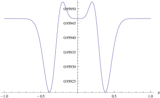
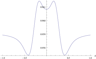
Figure 4: Plots of coverage probabilities $P_{n,\theta,\sigma}(\theta_{i}\in[\tilde{\theta}_{i}-\hat{\sigma}a_{i,n},\tilde{\theta}_{i}+\hat{\sigma}a_{i,n}]$ as a function of $\theta_{i}$ for hard-thresholding (left) and adaptive soft-thresholding (right), where $a_{i,n}$ was chosen for each estimator so that the upper bound in Proposition 14 and 18 equals $1-\alpha=0.95$. For both plots: $n=40$, $k=35$, $\eta_{i,n}=0.05$, $\xi_{i,n}=1$, $\sigma^{2}=1$.

6 Summary

We considered distributional properties of thresholding estimators within a normal linear regression model with a potentially diverging number of parameters where the error variance may be unknown. Aside from looking at finite-sample as well as large-sample distributions (within a moving-parameter asymptotic framework) for the estimators, we constructed valid confidence sets based on these estimators. We provided intervals that exactly have the prescribed coverage as their minimal coverage probability in finite samples for the case when the error variance is known, and conservative intervals where the minimal coverage probability can never fall below the prescribed value for the case of unknown error variance. Some numerical considerations were carried out to illustrate how conservative these lower bounds are and what the approximation entails for the lengths of the so-constructed intervals.

We showed that the lengths of the intervals based on the thresholding estimators are always larger compared to the corresponding standard intervals in finite samples. Asymptotically, in case of conservative variable selection, the lengths of all intervals including the standard one are of the same order. When the estimators are tuned to perform consistent variable selection, the lengths of the intervals based on the thresholding estimators are in fact larger by an order of magnitude compared to the standard one.

7 Acknowledgments

The author wishes to thank anonymous referees for very valuable comments and acknowledges support from DFG grant FOR 916.

Appendix A Overview of Assumptions and Results

A quick overview of the propositions and theorems derived in this paper is given below in Table 2. The first chart lists all finite-sample results. All of them except Theorem 12 concern the estimators for the case of unknown error variance. The second chart depicts asymptotic results under a conservatively tuned regime for the two cases of the asymptotic behavior of the number of degrees of freedom, namely, when $n-k$ eventually converges to a constant and when $n-k$ diverges. All results in this chart are for unknown error variance. Finally, the asymptotic results under a consistent variable selection framework are specified in the last chart. Proposition 13 concerns the known-variance case (for which the asymptotic behavior of $n-k$ is irrelevant), whereas all other results listed are for the unknown-variance case. Here, we distinguish three situations for the large-sample behavior of $n-k$: $n-k$ converging to a finite value, $n-k$ tending to infinity, and the subcase where $n-k$ diverges “fast enough” in relation to the tuning parameter $\eta_{i,n}$ in the sense that $n^{1/2}\eta_{i,n}/\sqrt{n-k}\to 0$. To contrast the main contributions of this paper concerning the confidence intervals with the auxiliary results on the distributions of the estimators, the former ones are listed in boldface.

finite-sample results
distributions	Prop. 3, 4, 5
confidence intervals	Ther. 12 (known variance)
	Prop. 14, 16, 18

asymptotic results: conservative tuning
	$n-k=m$	$n-k\to\infty$
distributions	Prop. 6, 7, 8	–
confidence intervals	–	Ther. 15, 17, 19

asymptotic results: consistent tuning
	$n-k=m$	$n-k\to\infty$	$\;\;n^{1/2}\eta_{i,n}/\sqrt{n-k}\to 0\;\;$
			($n-k\to\infty$ “fast enough”)
distributions	Prop. 9(a), 10(a), 11(a)	Prop. 9(b), 10(b), 11(b)
confidence intervals			Ther. 15, 17, 19
	Prop. 13 (known variance), Prop. 20

Table 2: Overview of assumptions and results.

Appendix B Proofs

B.1 Proofs for Section 3

Proof of Proposition 3.

In the following, we denote the distribution function of $\sigma^{-1}\alpha_{i,n}(\hat{\theta}_{H,i}-\theta_{i})$, the estimator in the known-variance case, by $H^{i}_{H,\eta_{i,n},n,\theta,\sigma}$ which was already derived in Pötscher & Schneider (2011). We have

$$\tilde{H}_{H,n,\theta,\sigma}^{i}(x) = \int_{0}^{\infty}P_{n,\theta,\sigma}\left(\sigma^{-1}\alpha_{i,n}(\tilde{\theta}_{H,i}-\theta_{i})\leq x\hat{\sigma}/\sigma\,\middle|\,\hat{\sigma}/\sigma=s\right)\rho_{n-k}(s)\,ds$$

$$= \int_{0}^{\infty}H^{i}_{H,s\eta_{i,n},n,\theta,\sigma}(xs)\,\rho_{n-k}(s)\,ds,$$

where we have used independence of $\hat{\sigma}$ and $\hat{\theta}_{LS,i}$ allowing us to replace $\hat{\sigma}$ by $s\sigma$ in the relevant formulas, cf. Leeb & Pötscher (2003, p. 110). Replacing $\eta_{i,n}$ by $s\eta_{i,n}$ and $x$ by $xs$ in (7) in Pötscher & Schneider (2011) into the above equation gives (5). To show (6) and (7), observe first that for each fixed $s$ we can regard $H^{i}_{H,s\eta_{i,n},n,\theta,\sigma}(xs)$ as $H^{i}_{H,s\eta_{i,n},n,\theta,\sigma}(x)$, but with the scaling factor $\alpha_{i,n}$ replaced by $\alpha_{i,n}/s$. Further rewriting this cdf as an integral of the measure $dH^{i}_{H,s\eta_{i,n},n,\theta,\sigma}$ from (8) in Pötscher & Schneider (2011), applying Fubini’s theorem and performing an elementary calculation yields

$$\tilde{H}^{i}_{H,n,\theta,\sigma}(x)\;=\;\int_{0}^{\infty}\boldsymbol{1}\{xs/\alpha_{i,n}+\theta_{i}/\sigma\geq 0\}$$

$$\times\left[\Phi\big{(}n^{1/2}(-\theta_{i}/(\sigma\xi_{i,n})+s\eta_{i,n})\big{)}-\Phi\big{(}n^{1/2}(-\theta_{i}/(\sigma\xi_{i,n})-s\eta_{i,n})\big{)}\right]\rho_{n-k}(s)\,ds$$

$$+\int_{-\infty}^{x}\int_{0}^{\infty}(n^{1/2}s/(\alpha_{i,n}\xi_{i,n}))\phi\big{(}n^{1/2}ws/(\alpha_{i,n}\xi_{i,n})\big{)}\boldsymbol{1}\left(|ws/\alpha_{i,n}+\theta_{i}/\sigma|>\xi_{i,n}s\eta_{i,n}\right)$$

$$\times\rho_{n-k}(s)\,dsdw$$

for any $\theta_{i}\in\mathbb{R}$. The second term in the above display immediately gives the second term in (6) and (7). Also, the first term in (6) can be derived in a straightforward manner since the indicator function in the first integral of the above display simply becomes $\boldsymbol{1}\{x\geq 0\}$ for $\theta_{i}=0$. Finally, to obtain the first term in (7), “move” the corresponding indicator function in the above display into the limits of the integral and differentiate with respect to to $x$ applying Leibniz’s integral rule.

Proof of Proposition 4.

The proof proceeds in a similar manner as in the proof of Proposition 3. Let $H^{i}_{S,\eta_{i,n},n,\theta,\sigma}$ denote the distribution function of $\sigma^{-1}\alpha_{i,n}(\hat{\theta}_{S,i}-\theta_{i})$, the estimator in the known-variance case, which was derived in Pötscher & Schneider (2011). We have

$$\tilde{H}_{S,n,\theta,\sigma}^{i}(x) = \int_{0}^{\infty}P_{n,\theta,\sigma}\left(\sigma^{-1}\alpha_{i,n}(\tilde{\theta}_{S,i}-\theta_{i})\leq x\hat{\sigma}/\sigma\,\middle|\,\hat{\sigma}/\sigma=s\right)\rho_{n-k}(s)\,ds$$

$$= \int_{0}^{\infty}H^{i}_{S,s\eta_{i,n},n,\theta,\sigma}(xs)\,\rho_{n-k}(s)\,ds,$$

where we have used independence of $\hat{\sigma}$ and $\hat{\theta}_{LS,i}$ allowing us to replace $\hat{\sigma}$ by $s\sigma$ in the relevant formulas, cf. Leeb & Pötscher (2003, p. 110). Replacing $\eta_{i,n}$ by $s\eta_{i,n}$ and $x$ by $xs$ in (9) in Pötscher & Schneider (2011) into the above equation gives (8). To show (9) and (10), observe first that for each fixed $s$ we can regard $H^{i}_{S,s\eta_{i,n},n,\theta,\sigma}(xs)$ as $H^{i}_{S,s\eta_{i,n},n,\theta,\sigma}(x)$, but with the scaling factor $\alpha_{i,n}$ replaced by $\alpha_{i,n}/s$. Further rewriting this cdf as an integral of the measure $dH^{i}_{S,s\eta_{i,n},n,\theta,\sigma}$ from (10) in Pötscher & Schneider (2011), applying Fubini’s theorem and performing an elementary calculation yields

$$\tilde{H}^{i}_{S,n,\theta,\sigma}(x)\;=\;\int_{0}^{\infty}\boldsymbol{1}\{xs/\alpha_{i,n}+\theta_{i}/\sigma\geq 0\}$$

$$\times\left[\Phi\big{(}n^{1/2}(-\theta_{i}/(\sigma\xi_{i,n})+s\eta_{i,n})\big{)}-\Phi\big{(}n^{1/2}(-\theta_{i}/(\sigma\xi_{i,n})-s\eta_{i,n})\big{)}\right]\rho_{n-k}(s)\,ds$$

$$+\int_{-\infty}^{x}\int_{0}^{\infty}(n^{1/2}s/(\alpha_{i,n}\xi_{i,n}))\left[\phi\big{(}n^{1/2}(ws/(\alpha_{i,n}\xi_{i,n})+s\eta_{i,n})\big{)}\boldsymbol{1}\left(ws/\alpha_{i,n}+\theta_{i}/\sigma>0\right)\right.$$

$$+\left.\phi\big{(}n^{1/2}(ws/(\alpha_{i,n}\xi_{i,n})-s\eta_{i,n})\big{)}\boldsymbol{1}\left(ws/\alpha_{i,n}+\theta_{i}/\sigma<0\right)\right]\rho_{n-k}(s)\,dsdw$$

for any $\theta_{i}\in\mathbb{R}$. The second term in the above display immediately gives the second term in (9) and (10). Also, the first term in (9) can be derived in a straightforward manner since the indicator function in the first integral of the above display simply becomes $\boldsymbol{1}\{x\geq 0\}$ for $\theta_{i}=0$. Finally, to obtain the first term in (10), “move” the corresponding indicator function in the above display into the limits of the integral and differentiate with respect to to $x$ applying Leibniz’s integral rule.

Proof of Proposition 5.

The proof proceeds in a similar manner as in the proof of Proposition 3. Let $H^{i}_{AS,\eta_{i,n},n,\theta,\sigma}$ denote the distribution function of $\sigma^{-1}\alpha_{i,n}(\hat{\theta}_{AS,i}-\theta_{i})$, the estimator in the known-variance case, which was derived in Pötscher & Schneider (2011). We have 4 that

$$\tilde{H}_{AS,n,\theta,\sigma}^{i}(x) = \int_{0}^{\infty}P_{n,\theta,\sigma}\left(\sigma^{-1}\alpha_{i,n}(\tilde{\theta}_{AS,i}-\theta_{i})\leq x\hat{\sigma}/\sigma\mid\hat{\sigma}=s\sigma\right)\rho_{n-k}(s)\,ds$$

$$= \int_{0}^{\infty}H^{i}_{AS,s\eta_{i,n},n,\theta,\sigma}(xs)\,\rho_{n-k}(s)\,ds,$$

where we have used independence of $\hat{\sigma}$ and $\hat{\theta}_{LS,i}$ allowing us to replace $\hat{\sigma}$ by $s\sigma$ in the relevant formulas, cf. Leeb & Pötscher (2003, p. 110). Replacing $\eta_{i,n}$ by $s\eta_{i,n}$ and $x$ by $xs$ in (11) in Pötscher & Schneider (2011) into the above equation gives (11). To show (12) and (13), observe first that for each fixed $s$ we can write $H^{i}_{AS,s\eta_{i,n},n,\theta,\sigma}(xs)$ as $H^{i}_{AS,s\eta_{i,n},n,\theta,\sigma}(x)$, but with the scaling factor $\alpha_{i,n}$ replaced by $\alpha_{i,n}/s$. Further rewriting this cdf as an integral of the measure $dH^{i}_{AS,s\eta_{i,n},n,\theta,\sigma}$ from Proposition 21 in Pötscher & Schneider (2011), applying Fubini’s theorem and performing an elementary calculation yields

$$\tilde{H}^{i}_{AS,n,\theta,\sigma}(x)\;=\;\int_{0}^{\infty}\boldsymbol{1}\{xs/\alpha_{i,n}+\theta_{i}/\sigma\geq 0\}$$

$$\times\left[\Phi\big{(}n^{1/2}(-\theta_{i}/(\sigma\xi_{i,n})+s\eta_{i,n})\big{)}-\Phi\big{(}n^{1/2}(-\theta_{i}/(\sigma\xi_{i,n})-s\eta_{i,n})\big{)}\right]\rho_{n-k}(s)\,ds$$

$$+\int_{-\infty}^{x}\int_{0}^{\infty}0.5(n^{1/2}s/(\alpha_{i,n}\xi_{i,n}))\left[\phi\big{(}z_{n,\theta,\sigma}^{(2)}(ws,s\eta_{i,n})\big{)}(1+t_{n,\theta,\sigma}(ws,s\eta_{i,n}))\boldsymbol{1}\{ws/\alpha_{i,n}+\theta_{i}/\sigma>0\}\right.$$

$$+\phi\big{(}z_{n,\theta,\sigma}^{(1)}(ws,s\eta_{i,n})\big{)}(1-t_{n,\theta,\sigma}(ws,s\eta_{i,n}))\boldsymbol{1}\{ws/\alpha_{i,n}+\theta_{i}/\sigma<0\}\left.\right]\rho_{n-k}(s)\,ds\,dw$$

for any $\theta_{i}\in\mathbb{R}$. The second term in the above display immediately gives the second term in (12) and (13). Also, the first term in (12) can also be derived in a straightforward manner since the indicator function in the first integral of the above display simply becomes $\boldsymbol{1}\{x\geq 0\}$ for $\theta_{i}=0$. Finally, to obtain the first term in (13), “move” the corresponding indicator function in the above display into the limits of the integral and differentiate with respect to to $x$ applying Leibniz’s integral rule.

B.2 Proofs for Section 4

Proof of Proposition 6.

Note that for fixed $x$ the expression inside the square brackets in (5) converges to the expression inside the square brackets in (14) for Lebesgue-almost all $s\in(0,\infty)$. Since $n-k=m$ eventually, the dominated convergence theorem proves (14). To conclude the expressions for the corresponding measure, note that the limit distribution in (14) is the same as the finite-sample distribution in (5) with $n^{1/2}\theta_{i,n}/(\sigma_{n}\xi_{i,n})$ and $n^{1/2}\eta_{i,n}$ having settled down to their limiting values $\nu_{i}$ and $e_{i}$, respectively, so that the formulas in (6) and (7) can be used.

Proof of Proposition 7.

The proof proceeds in a similar manner as the proof of Proposition 6. Note that for fixed $x$ the expression inside the square brackets in (8) converges to the expression inside the square brackets in (15) for Lebesgue-almost all $s\in(0,\infty)$. Since $n-k=m$ eventually, the dominated convergence theorem proves (15). To conclude the expressions for the corresponding measure, note that the limit distribution in (15) is the same as the finite-sample distribution in (8) with $n^{1/2}\theta_{i,n}/(\sigma_{n}\xi_{i,n})$ and $n^{1/2}\eta_{i,n}$ having settled down to their limiting values $\nu_{i}$ and $e_{i}$, respectively, so that the formulas in (9) and (10) can be used.

Proof of Proposition 8.

The proof proceeds in a similar manner as the proof of Proposition 6. Note that for fixed $x$ the expression inside the square brackets in (11) converges to the expression inside the square brackets in (16) for Lebesgue-almost all $s\in(0,\infty)$. Since $n-k=m$ eventually, the dominated convergence theorem proves (16). To conclude the expressions for the corresponding measure, note that the limit distribution in (16) is the same as the finite-sample distribution in (11) with $n^{1/2}\theta_{i,n}/(\sigma_{n}\xi_{i,n})$ and $n^{1/2}\eta_{i,n}$ having settled down to their limiting values $\nu_{i}$ and $e_{i}$, respectively, so that the formulas in (12) and (13) can be used.

Proof of Proposition 9.

To prove part (a) note that by Proposition 3 the distribution function of $(\hat{\sigma}\xi_{i,n}\eta_{i,n})^{-1}(\tilde{\theta}_{H,i}-\theta_{i,n})$ is given by

$$\begin{split}\int_{0}^{\infty}\big{[}\Phi\big{(}n^{1/2}\eta_{i,n}xs\big{)}\boldsymbol{1}\big{(}&|xs+\zeta_{i,n}|>s\big{)}+\Phi\big{(}n^{1/2}\eta_{i,n}(s-\zeta_{i,n})\big{)}\boldsymbol{1}\left(0\leq xs+\zeta_{i,n}\leq s\right)\\ &+\Phi\big{(}n^{1/2}\eta_{i,n}(-s-\zeta_{i,n})\big{)}\boldsymbol{1}\left(-s\leq xs+\zeta_{i,n}<0\right)\big{]}\rho_{n-k}(s)\,ds,\end{split}$$ (20)

where $\zeta_{i,n}=\theta_{i,n}/(\sigma_{n}\xi_{i,n}\eta_{i,n})$ and $\zeta_{i,n}\to\zeta_{i}$. Since $n^{1/2}\eta_{i,n}\to\infty$ and $n-k=m$ eventually, the dominated convergence theorem gives that the above display converges to

$$\begin{split}\int_{0}^{\infty}\big{[}\boldsymbol{1}(x\geq 0)\boldsymbol{1}(|xs+\zeta_{i}|&>s)+\boldsymbol{1}(s>\zeta_{i})\boldsymbol{1}(0\leq xs+\zeta_{i}\leq s)\\ &+\boldsymbol{1}(s<-\zeta_{i})\boldsymbol{1}(-s\leq xs+\zeta_{i}<0)\big{]}\rho_{m}(s)\,ds\end{split}$$ (21)

for all $x\neq 0$ since then the integrand of (20) converges to the integrand of (21) for Lebesgue-almost all $s>0$. The expression in (21) clearly simplifies to $\boldsymbol{1}(x\geq 0)$ when $|\zeta_{i}|=\infty$ or $\zeta_{i}=0$, proving part 1. For $0<|\zeta_{i}|<\infty$, after some elementary calculations, we can write (21) as

$$\boldsymbol{1}(-1\leq x<0)\int_{\zeta_{i}}^{-\zeta_{i}/x}\rho_{m}(s)\,ds+\boldsymbol{1}(x\geq 0)$$

when $\zeta_{i}>0$, and as

$$\boldsymbol{1}(0\leq x<1)\big{[}\int_{-\zeta_{i}/x}^{\infty}\rho_{m}(s)\,ds+\int_{0}^{-\zeta_{i}}\rho_{m}(s)\,ds\big{]}+\boldsymbol{1}(x\geq 1)$$

when $\zeta_{i}<0$, yielding 2. and 3. and finishing the proof for part (a).

For proving part (b), note that the distribution corresponding to $\rho_{n-k}$, that is, the distribution of $\hat{\sigma}/\sigma_{n}$, now converges to pointmass at 1 in probability. This implies that by Slutzky’s Theorem the limiting distribution of $\hat{\sigma}^{-1}\alpha_{i,n}(\tilde{\theta}_{H,i}-\theta_{i,n})=(\hat{\sigma}/\sigma_{n})^{-1}\,\sigma_{n}^{-1}\alpha_{i,n}(\tilde{\theta}_{H,i}-\theta_{i,n})$ is the same as the one of $\sigma_{n}^{-1}\alpha_{i,n}(\tilde{\theta}_{H,i}-\theta_{i,n})$ which can be found in Theorem 36(b) in Pötscher & Schneider (2011).

Proof of Proposition 10.

To prove part (a) note that the cdf of $\hat{\sigma}^{-1}\alpha_{i,n}(\tilde{\theta}_{S,i}-\theta_{i,n})$ with $\alpha_{i,n}=(\xi_{i,n}\eta_{i,n})^{-1}$ is given by

$$\int_{0}^{\infty}\big{[}\Phi\big{(}n^{1/2}\eta_{i,n}(x+1)s)\big{)}\boldsymbol{1}\left(xs+\zeta_{i,n}\geq 0\right)+\Phi\big{(}n^{1/2}\eta_{i,n}(x-1)s\big{)}\boldsymbol{1}\left(xs+\zeta_{i,n}<0\right)\big{]}\rho_{n-k}(s)\,ds,$$ (22)

again, where $\zeta_{i,n}=\theta_{i,n}/(\sigma_{n}\xi_{i,n}\eta_{i,n})$ and $\zeta_{i,n}\to\zeta_{i}$. Since $n^{1/2}\eta_{i,n}\to\infty$ and $n-k=m$ eventually, the dominated convergence theorem gives that the above display converges to

$$\int_{0}^{\infty}\big{[}\boldsymbol{1}(x\geq-1)\boldsymbol{1}(xs+\zeta_{i}\geq 0)+\boldsymbol{1}(x\geq 1)\boldsymbol{1}(xs+\zeta_{i}<0)\big{]}\rho_{m}(s)\,ds,$$ (23)

for all $x\neq-1$ when $\zeta_{i}>0$, for all $x\neq 1$ when $\zeta_{i}<0$, and for all $x\neq 0$ when $\zeta_{i}=0$, since then the integrand of (22) converges to the integrand of (23) for Lebesgue-almost all $s>0$. The expression in (23) simplifies to $\boldsymbol{1}(x\geq-1)$ and $\boldsymbol{1}(x\geq 1)$ for $\zeta_{i}=\infty$ and $\zeta_{i}=-\infty$, respectively, and to $\boldsymbol{1}(x\geq 0)$ for $\zeta_{i}=0$, proving parts 1. and 3. For $0<|\zeta_{i}|<\infty$, we can write (23) as

$$\boldsymbol{1}(-1\leq x<0)\int_{0}^{-\zeta_{i}/x}\rho_{m}(s)\,ds+\boldsymbol{1}(x\geq 0)$$

when $\zeta_{i}>0$, and as

$$\boldsymbol{1}(0\leq x<1)\int_{-\zeta_{i}/x}^{\infty}\rho_{m}(s)\,ds+\boldsymbol{1}(x\geq 1)$$

when $\zeta_{i}<0$, yielding 2. and 4. and finishing the proof for part (a).

For proving part (b), note that the distribution corresponding to $\rho_{n-k}$, that is, the distribution of $\hat{\sigma}/\sigma_{n}$, now converges to pointmass at 1 in probability. This implies that by Slutzky’s Theorem the limiting distribution of $\hat{\sigma}^{-1}\alpha_{i,n}(\tilde{\theta}_{S,i}-\theta_{i,n})=(\hat{\sigma}/\sigma_{n})^{-1}\,\sigma_{n}^{-1}\alpha_{i,n}(\tilde{\theta}_{S,i}-\theta_{i,n})$ is the same as the one of $\sigma_{n}^{-1}\alpha_{i,n}(\tilde{\theta}_{S,i}-\theta_{i,n})$ which can be found in Theorem 37(b) in Pötscher & Schneider (2011).

Proof of Proposition 11.

To prove part (a) note that the cdf of $\hat{\sigma}^{-1}\alpha_{i,n}(\tilde{\theta}_{AS,i}-\theta_{i,n})$ with $\alpha_{i,n}=(\xi_{i,n}\eta_{i,n})^{-1}$ can be written as

$$\begin{split}\int_{0}^{\infty}&\big{[}\Phi\big{(}n^{1/2}\eta_{i,n}\big{(}(xs-\zeta_{i,n})/2+\sqrt{((xs+\zeta_{i,n})/2)^{2}+s^{2}}\big{)}\big{)}\boldsymbol{1}\left(xs+\zeta_{i,n}\geq 0\right)\\ &+\;\Phi\big{(}n^{1/2}\eta_{i,n}\big{(}(xs-\zeta_{i,n})/2-\sqrt{((xs+\zeta_{i,n})/2)^{2}+s^{2}}\big{)}\big{)}\boldsymbol{1}\left(xs+\zeta_{i,n}<0\right)\big{]}\rho_{n-k}(s)\,ds,\end{split}$$ (24)

again, where $\zeta_{i,n}=\theta_{i,n}/(\sigma_{n}\xi_{i,n}\eta_{i,n})$ and $\zeta_{i,n}\to\zeta_{i}$. Since $n^{1/2}\eta_{i,n}\to\infty$ and $n-k=m$ eventually, the dominated convergence theorem gives that the above display converges to

$$\begin{split}\int_{0}^{\infty}&\big{[}\boldsymbol{1}\big{(}(xs-\zeta_{i})/2+\sqrt{((xs+\zeta_{i})/2)^{2}+s^{2}}\geq 0\big{)}\boldsymbol{1}(xs+\zeta_{i}\geq 0)\\ &+\;\boldsymbol{1}\big{(}(xs-\zeta_{i})/2-\sqrt{((xs+\zeta_{i})/2)^{2}+s^{2}}\geq 0\big{)}\boldsymbol{1}(xs+\zeta_{i}<0)\big{]}\rho_{m}(s)\,ds,\end{split}$$ (25)

for all $x$ when $0<|\zeta_{i}|<\infty$, and for all $x\neq 0$ when $\zeta_{i}=0$, since then the integrand of (24) converges to the integrand of (25) for Lebesgue-almost all $s>0$. The expression simplifies to $\boldsymbol{1}(x\geq 0)$ for $\zeta_{i}=0$. To find the limit when $|\zeta_{i}|=\infty$, we first consider the case $\zeta_{i}=\infty$. For large enough $n$, the integrand in (24) becomes $\boldsymbol{1}((xs-\zeta_{i,n})/2+\sqrt{((xs+\zeta_{i,n})/2)^{2}+s^{2}}\geq 0)$ so that we need to determine the limit of

$$\big{(}(xs -\zeta_{i,n})/2\big{)}+\sqrt{\big{(}(xs+\zeta_{i,n})/2\big{)}^{2}+s^{2}}$$

$$=\;\big{(}(xs-\zeta_{i,n})/2\big{)}+\big{(}(xs+\zeta_{i,n})/2\big{)}\sqrt{1+\big{(}2s/(xs+\zeta_{i,n})\big{)}^{2}}$$

$$=\;\big{(}(xs-\zeta_{i,n})/2\big{)}+\big{(}(xs+\zeta_{i,n})/2\big{)}\big{(}1+O\big{(}(s/(xs+\zeta_{i,n})^{2}\big{)}\big{)}$$

$$=\;xs+o(1)$$

as $\zeta_{i,n}\to\infty$, where we have used a Taylor-expansion of $\sqrt{1+z}$ around 0. We can therefore conclude that for all fixed $x\neq 0$, the integrand of (24) converges for Lebesgue-almost all $s>0$ to $\boldsymbol{1}(xs\geq 0)$ implying that the weak limit of (24) is $\boldsymbol{1}(x\geq 0)$. The proof for $\zeta_{i}=-\infty$ works analogously, finishing part 1.

For $0<|\zeta_{i}|<\infty$, a tedious but elementary case-by-case analysis shows that we can write (25) as

$$\boldsymbol{1}(-1\leq x<0)\int_{-x\zeta_{i}}^{-\zeta_{i}/x}\rho_{m}(s)\,ds+\boldsymbol{1}(x\geq 0)$$

when $\zeta_{i}>0$, and as

$$\boldsymbol{1}(0\leq x<1)\big{[}\int_{-\zeta_{i}/x}^{\infty}\rho_{m}(s)\,ds+\int_{0}^{-\zeta_{i}x}\rho_{m}(s)\,ds\big{]}+\boldsymbol{1}(x\geq 1)$$

when $\zeta_{i}<0$, yielding 2. and 3. and finishing the proof for part (a).

For proving part (b), note that the distribution corresponding to $\rho_{n-k}$, that is, the distribution of $\hat{\sigma}/\sigma_{n}$, now converges to pointmass at 1 in probability. This implies that by Slutzky’s Theorem the limiting distribution of $\hat{\sigma}^{-1}\alpha_{i,n}(\tilde{\theta}_{AS,i}-\theta_{i,n})=(\hat{\sigma}/\sigma_{n})^{-1}\,\sigma_{n}^{-1}\alpha_{i,n}(\tilde{\theta}_{AS,i}-\theta_{i,n})$ is the same as the one of $\sigma_{n}^{-1}\alpha_{i,n}(\tilde{\theta}_{AS,i}-\theta_{i,n})$ which can be found in Theorem 38(b) in Pötscher & Schneider (2011).

B.3 Proofs for Section 5

Proof of Theorem 12.

We first consider the hard-thresholding estimator. Observe that

$$\hat{\theta}_{H,i}/(\sigma\xi_{i,n})=\left(\hat{\theta}_{LS,i}/(\sigma\xi_{i,n})\right)\boldsymbol{1}\left(|\hat{\theta}_{LS,i}/(\sigma\xi_{i,n})|>\eta_{i,n}\right)$$

and that $\hat{\theta}_{LS,i}/(\sigma\xi_{i,n})$ is $N(\theta_{i}/(\sigma\xi_{i,n}),1/n)$. Pötscher & Schneider (2010) derive confidence intervals for a hard-thresholding estimator for a Gaussian linear regression model with orthogonal regressors and known error variance. Identifying $\hat{\theta}_{LS,i}/(\sigma\xi_{i,n})$ and $\theta_{i}/(\sigma\xi_{i,n})$ with $\bar{y}$ and $\theta$ and making use of Proposition 2 and Theorem 5 in the above reference by noting that

$$P_{n,\theta,\sigma} \left(\theta_{i}\in[\hat{\theta}_{H,i}-\sigma a_{i,n},\hat{\theta}_{H,i}+\sigma b_{i,n}]\right)$$

$$=\;P_{n,\theta,\sigma}\left(\theta_{i}/(\sigma\xi_{i,n})\in\left[\hat{\theta}_{H,i}/(\sigma\xi_{i,n})-a_{i,n}/\xi_{i,n},\hat{\theta}_{H,i}/(\sigma\xi_{i,n})+b_{i,n}/\xi_{i,n}\right]\right)$$

immediately gives the result in (a) after replacing $\eta_{n}$ with $\eta_{i,n}$ and $a_{n}$ by $a/\xi_{i,n}$. The results for soft- and adaptive soft-thresholding in (b) and (c), respectively, follow analogously by making use of Proposition 1 and 3, respectively, as well as Theorem 5 in the reference mentioned above.

Proof of Proposition 13.

Note that

$$P_{n,\theta,\sigma}(\theta_{i}\in D_{i,n})=P_{n,\theta,\sigma}\left(-d\leq(\sigma\xi_{i,n}\eta_{i,n})^{-1}(\hat{\theta}_{i}-\theta_{i})\leq d\right).$$

Propositions 27(b), 28(b), and 29(b) in Pötscher & Schneider (2011) show that any accumulation point of the limiting distribution of $(\sigma\xi_{i,n}\eta_{i,n})^{-1}(\hat{\theta}_{i}-\theta_{i})$ with respect to weak convergence is a measure concentrated on $[-1,1]$, which proves the result for $d>1$. If $d<1$, the same propositions show that we can always find a sequence $\theta^{(n)}$ such that the distribution of $(\sigma\xi_{i,n}\eta_{i,n})^{-1}(\hat{\theta}_{i}-\theta_{i,n})$ is concentrated on one of the endpoints of the interval $[-1,1]$ implying

$$P_{n,\theta,\sigma}\left(-d\leq(\xi_{i,n}\eta_{i,n})^{-1}(\hat{\theta}_{i}-\theta_{i,n})\leq d\right)\longrightarrow 0$$

and proving the claim for $d<1$. Finally, use the expressions for the infimal coverage probabilities in Theorem 12 to see the result for $d=1/2$.

Proof of Proposition 14.

Define $p^{i}_{H,n}(\theta,\sigma,a_{i,n},\eta_{i,n})=P_{n,\theta,\sigma}(\theta_{i}\in C_{H,i,n})$, the coverage probability for the hard-thresholding estimator with known error variance. As discussed in the beginning of Section 5.2, we have

$$\inf_{\theta\in\mathbb{R},\sigma\in\mathbb{R}_{+}} P_{n,\theta,\sigma}(\theta\in E_{H,i,n})=\inf_{\theta\in\mathbb{R}}\int_{0}^{\infty}p^{i}_{H,n}(\theta,1,a_{i,n}s,\eta_{i,n}s)\rho_{n-k}(s)\,ds$$

$$\geq\;\int_{0}^{\infty}\inf_{\theta\in\mathbb{R}}p^{i}_{H,n}(\theta,1,a_{i,n}s,\eta_{i,n}s)\rho_{n-k}(s)\,ds$$

which equals

$$\int_{0}^{\infty}\big{[}\Phi(n^{1/2} (a_{i,n}/\xi_{i,n}-\eta_{i,n})s)-\Phi(-n^{1/2}a_{i,n}s/\xi_{i,n})\big{]}\rho_{n-k}(s)\,ds$$

$$=\;T_{n-k}(n^{1/2}(a_{i,n}/\xi_{i,n}-\eta_{i,n}))-T_{n-k}(-n^{1/2}a_{i,n}/\xi_{i,n})$$

when $a_{i,n}\geq\xi_{i,n}\eta_{i,n}/2$, and 0 for $a_{i,n}<\xi_{i,n}\eta_{i,n}/2$, cf. Theorem 12(a).

Proof of Theorem 15.

For $p^{i}_{H,n}(\theta,\sigma,a_{i,n},\eta_{i,n})=p^{i}_{H,n}(\theta/\sigma,1,a_{i,n},\eta_{i,n})=P_{n,\theta,\sigma}(\theta_{i}\in C_{H,i,n})$, the coverage probability in the known-variance case, we have

$$\lim_{\theta_{i}\to\infty}p^{i}_{H,n}(\theta,1,a_{i,n},\eta_{i,n})=\Phi(n^{1/2}a_{i,n}/\xi_{i,n})-\Phi(-n^{1/2}a_{i,n}/\xi_{i,n}),$$

as can be seen from Proposition 19 in Pötscher & Schneider (2011). This implies that

$$\inf_{\theta\in\mathbb{R}^{k}}P_{n,\theta,\sigma}(\theta_{i}\in C_{H,i,n})\leq\Phi(n^{1/2}a_{i,n}/\xi_{i,n})-\Phi(-n^{1/2}a_{i,n}/\xi_{i,n}),$$ (26)

as well as

$$\inf_{\theta\in\mathbb{R}^{k},\sigma\in\mathbb{R}_{+}} P_{n,\theta,\sigma}(\theta_{i}\in E_{H,i,n})\leq\lim_{\theta_{i}\to\infty}\int_{0}^{\infty}p^{i}_{H,n}(\theta,1,a_{i,n}s,\eta_{i,n}s)\rho_{n-k}(s)\,ds$$

$$=\;\int_{0}^{\infty}\left[\Phi(n^{1/2}a_{i,n}s/\xi_{i,n})-\Phi(-n^{1/2}a_{i,n}s/\xi_{i,n})\right]\rho_{n-k}(s)\,ds$$

$$=\;T_{n-k}(n^{1/2}a_{i,n}/\xi_{i,n})-T_{n-k}(-n^{1/2}a_{i,n}/\xi_{i,n}),$$ (27)

where we have used dominated convergence for the first equality in the above display.

Step 1: If $n^{1/2}a_{i,n}/\xi_{i,n}\to 0$, the upper bounds in (26) and (27) both converge to 0, thus proving the claim.

Step 2: Let $n^{1/2}\eta_{i,n}\to 0$. If $a_{i,n}<\xi_{i,n}\eta_{i,n}/2$, then $n^{1/2}a_{i,n}/\xi_{i,n}\to 0$ also, showing the theorem by Step 1. If $a_{i,n}\geq\xi_{i,n}\eta_{i,n}/2$, we have by Theorem 12(a) that $\inf_{\theta\in\mathbb{R}^{k}}P_{n,\theta,\sigma}(\theta_{i}\in C_{H,i,n})$ differs from $\Phi(n^{1/2}a_{i,n}/\xi_{i,n})-\Phi(-n^{1/2}a_{i,n}/\xi_{i,n})$ only by a term that is $o(1)$ since $\Phi$ is globally Lipschitz. The same is true for $\inf_{\theta\in\mathbb{R}^{k},\sigma\in\mathbb{R}_{+}}P_{n,\theta,\sigma}(\theta_{i}\in E_{H,i,n})$ since then the difference between lower bound from Proposition 14 and the upper bound from (27) converges to zero, so that $|\inf_{\theta\in\mathbb{R}^{k},\sigma\in\mathbb{R}_{+}}P_{n,\theta,\sigma}(\theta_{i}\in E_{H,i,n})-[\Phi(n^{1/2}a_{i,n}/\xi_{i,n})-\Phi(-n^{1/2}a_{i,n}/\xi_{i,n})]|\leq o(1)+2\|\Phi-T_{n-k}\|_{\infty}\to 0$ by Polya’s Theorem.

Step 3: Assume $n^{1/2}(a_{i,n}/\xi_{i,n}-\eta_{i,n})\to\infty$. We then have $n^{1/2}a_{i,n}/\xi_{i,n}\to\infty$ also, so that by Theorem 12(a) together with Proposition 14 the infimal coverage probabilities both converge to 1, showing the claim for this step.

Step 4: By a subsequence argument we may now assume that $n^{1/2}a_{i,n}/\xi_{i,n}$ as well as $n^{1/2}\eta_{i,n}$ are bounded away from zero, and that $n^{1/2}(a_{i,n}/\xi_{i,n}-\eta_{i,n})$ is bounded from above. Note that this implies that $a_{i,n}/(\xi_{i,n}\eta_{i,n})$ is also bounded from above by some constant, say, $C$. By Lemma 13 in Pötscher & Schneider (2010) [after identifying $n$ with $n-k$ and $h_{n}$ with $\rho_{n-k}$] we see that for every $\varepsilon>0$ we can find a constant $c(\varepsilon)>0$ such that for every $n\geq 2$

$$\int_{1-c(\varepsilon)(n-k)^{-1/2}}^{1+c(\varepsilon)(n-k)^{-1/2}}\rho_{n-k}(s)\,ds\geq 1-\varepsilon.$$ (28)

Now define $\theta^{(n)}(\varepsilon)$ to have $i$-th component $\theta_{i,n}(\varepsilon):=a_{i,n}(1+c(\varepsilon)(n-k)^{-1/2})$ and set the remaining components to arbitrary values. By Proposition 19 in Pötscher & Schneider (2011), this choice of $\theta^{(n)}$ implies that for large enough $n$ we have

$$|p^{i}_{H,n}(\theta^{(n)}(\varepsilon),1,a_{i,n},\eta_{i,n})-\inf_{\theta\in\mathbb{R}^{k}}p^{i}_{H,n}(\theta,1,a_{i,n},\eta_{i,n})|$$

$$=\;|\max(0,\Phi(n^{1/2}(\theta_{i,n}(\varepsilon)/\xi_{i,n}-\eta_{i,n}))-\Phi(-n^{1/2}a_{i,n}/\xi_{i,n}))$$

$$\;\;\;\;\;\;-\max(0,\Phi(n^{1/2}(a_{i,n}/\xi_{i,n}-\eta_{i,n}))-\Phi(-n^{1/2}a_{i,n}/\xi_{i,n}))|$$

$$\leq\;(2\pi)^{-1/2}n^{1/2}|\theta_{i,n}(\varepsilon)/\xi_{i,n}-a_{i,n}/\xi_{i,n}|=(2\pi)^{-1/2}c(\varepsilon)(n-k)^{-1/2}n^{1/2}a_{i,n}/\xi_{i,n}$$

$$\leq\;(2\pi)^{-1/2}c(\varepsilon)Cn^{1/2}\eta_{i,n}/(n-k)^{1/2}\longrightarrow 0,$$

where we have used the fact that $\max(0,x)$ is globally Lipschitz with constant 1 and $\Phi(x)$ is globally Lipschitz with constant $(2\pi)^{-1/2}$. Moreover, for $s$ satisfying $|s-1|<c(\varepsilon)(n-k)^{-1/2}$ we have by the boundedness of $a_{i,n}/(\xi_{i,n}\eta_{i,n})$ that $sa_{i,n}<\theta_{i,n}(\varepsilon)\leq s(a_{i,n}+\xi_{i,n}\eta_{i,n})$ for large enough $n$. For such $s$ and $n$, this implies, in a similar manner as above,

$$| p^{i}_{H,n}(\theta^{(n)}(\varepsilon),1,a_{i,n}s,\eta_{i,n}s)-p^{i}_{H,n}(\theta^{(n)}(\varepsilon),1,a_{i,n},\eta_{i,n})|$$

$$=\;|\max(0,\Phi(n^{1/2}(\theta_{i,n}(\varepsilon)/\xi_{i,n}-\eta_{i,n}s))-\Phi(-n^{1/2}a_{i,n}s/\xi_{i,n}))$$

$$\;\;\;\;\;\;-\max(0,\Phi(n^{1/2}(\theta_{i,n}(\varepsilon)/\xi_{i,n}-\eta_{i,n}))-\Phi(-n^{1/2}a_{i,n}/\xi_{i,n}))|$$

$$\leq\;(2\pi)^{-1/2}|s-1|n^{1/2}(a_{i,n}/\xi_{i,n}+\eta_{i,n})$$

$$\leq\;(2\pi)^{-1/2}c(\varepsilon)(1+C)n^{1/2}\eta_{i,n}/(n-k)^{1/2}\longrightarrow 0.$$

This furthermore entails that

$$\inf_{\theta\in\mathbb{R},\sigma\in\mathbb{R}_{+}}P_{n,\theta,\sigma}(\theta_{i}\in E_{H,i,n})\;\leq\;\int_{0}^{\infty}p^{i}_{H,n}(\theta_{n}(\varepsilon),1,a_{i,n}s,\eta_{i,n}s)\rho_{n-k}(s)\,ds$$

$$\leq\;\int_{0}^{\infty}\left|p^{i}_{H,n}(\theta_{n}(\varepsilon),1,a_{i,n}s,\eta_{i,n}s)-p^{i}_{H,n}(\theta^{(n)}(\varepsilon),1,a_{i,n},\eta_{i,n})\right|\rho_{n-k}(s)\,ds$$

$$\;\;\;\;\;\;\;\;\;+p^{i}_{H,n}(\theta^{(n)}(\varepsilon),1,a_{i,n},\eta_{i,n})$$

$$\leq\;\int_{1-c(\varepsilon)(n-k)^{-1/2}}^{1+c(\varepsilon)(n-k)^{-1/2}}\left|p^{i}_{H,n}(\theta_{n}(\varepsilon),1,a_{i,n}s,\eta_{i,n}s)-p^{i}_{H,n}(\theta^{(n)}(\varepsilon),1,a_{i,n},\eta_{i,n})\right|\rho_{n-k}(s)\,ds$$

$$\;\;\;\;\;\;\;\;\;+\varepsilon+p^{i}_{H,n}(\theta^{(n)}(\varepsilon),1,a_{i,n},\eta_{i,n})$$

$$=\;\inf_{\theta\in\mathbb{R}^{k}}p^{i}_{H,n}(\theta,1,a_{i,n},\eta_{i,n})+\varepsilon+o(1)=\;\inf_{\theta\in\mathbb{R}^{k}}P_{n,\theta,\sigma}(\theta_{i}\in C_{H,i,n})+\varepsilon+o(1),$$

where we have made use of (28) and $\varepsilon>0$ was arbitrary. On the other hand, Proposition 14 and Theorem 12(a) show that

$$\inf_{\theta\in\mathbb{R}^{k},\sigma\in\mathbb{R}_{+}} P_{n,\theta,\sigma}(\theta_{i}\in E_{H,i,n})\geq\max[0,T_{n-k}(n^{1/2}(a_{i,n}/\xi_{i,n}-\eta_{i,n}))-T_{n-k}(-n^{1/2}a_{i,n}/\xi_{i,n})]$$

$$\geq\;\max[0,\Phi(n^{1/2}(a_{i,n}/\xi_{i,n}-\eta_{i,n}))-\Phi(-n^{1/2}a_{i,n}/\xi_{i,n})]-2\|\Phi-T_{n-k}\|_{\infty}$$

$$=\;\inf_{\theta\in\mathbb{R}^{k}}P_{n,\theta,\sigma}(\theta_{i}\in C_{H,i,n})-2\|\Phi-T_{n-k}\|_{\infty},$$

where $\|\Phi-T_{n-k}\|_{\infty}\to 0$ when $n-k\to\infty$ by Polya’s Theorem, finally proving the claim.

Proof of Proposition 16.

Define $p^{i}_{S,n}(\theta,\sigma,a_{i,n},\eta_{i,n})=P_{n,\theta,\sigma}(\theta_{i}\in[\hat{\theta}_{S,i}-\sigma a_{i,n},\hat{\theta}_{S,i}-\sigma a_{i,n}])$, the coverage probability for the soft-thresholding estimator with known error variance. We have

$$T_{n-k}(n^{1/2}(a_{i,n}/\xi_{i,n}-\eta_{i,n}))-T_{n-k}(n^{1/2}(-a_{i,n}/\xi_{i,n}-\eta_{i,n}))$$

$$=\;\int_{0}^{\infty}\big{[}\Phi(n^{1/2}(a_{i,n}/\xi_{i,n}-\eta_{i,n})s)-\Phi(n^{1/2}(-a_{i,n}/\xi_{i,n}-\eta_{i,n})s)\big{]}\rho_{n-k}(s)\,ds$$

$$=\int_{0}^{\infty}\lim_{\theta_{i}\to\infty}p^{i}_{S,n}(\theta,1,a_{i,n}s,\eta_{i,n}s)\rho_{n-k}(s)\,ds=\lim_{\theta_{i}\to\infty}\int_{0}^{\infty}p^{i}_{S,n}(\theta,1,a_{i,n}s,\eta_{i,n}s)\rho_{n-k}(s)\,ds$$

$$\geq\;\inf_{\theta\in\mathbb{R}^{k}}P_{n,\theta,1}(\theta_{i}\in E_{S,i,n})\;\geq\;\int_{0}^{\infty}\inf_{\theta\in\mathbb{R}^{k}}p^{i}_{S,n}(\theta,1,a_{i,n}s,\eta_{i,n}s)\rho_{n-k}(s)\,ds$$

$$=\;\int_{0}^{\infty}\big{[}\Phi(n^{1/2}(a_{i,n}/\xi_{i,n}-\eta_{i,n})s)-\Phi(n^{1/2}(-a_{i,n}/\xi_{i,n}-\eta_{i,n})s)\big{]}\rho_{n-k}(s)\,ds$$

$$=\;T_{n-k}(n^{1/2}(a_{i,n}/\xi_{i,n}-\eta_{i,n}))-T_{n-k}(n^{1/2}(-a_{i,n}/\xi_{i,n}-\eta_{i,n})),$$

where the second equality can be seen from Proposition 20 in Pötscher & Schneider (2011), the third equality is due to dominated convergence, and the second-last equality comes from Theorem 12(b).

Proof of Proposition 18.

Define $p^{i}_{AS,n}(\theta,\sigma,a_{i,n},\eta_{i,n})=P_{n,\theta,\sigma}(\theta_{i}\in[\hat{\theta}_{AS,i}-\sigma a_{i,n},\hat{\theta}_{AS,i}-\sigma a_{i,n}])$, the coverage probability for the adaptive soft-estimator with known error variance. As discussed in the beginning of Section 5.2, we have

$$\inf_{\theta\in\mathbb{R},\sigma\in\mathbb{R}_{+}} P_{n,\theta,\sigma}(\theta_{i}\in E_{AS,i,n})=\inf_{\theta\in\mathbb{R}^{k}}\int_{0}^{\infty}p^{i}_{AS,n}(\theta,1,a_{i,n}s,\eta_{i,n}s)\rho_{n-k}(s)\,ds$$

$$\geq\;\int_{0}^{\infty}\inf_{\theta\in\mathbb{R}^{k}}p^{i}_{AS,n}(\theta,1,a_{i,n}s,\eta_{i,n}s)\rho_{n-k}(s)\,ds$$

$$=\;\int_{0}^{\infty}\big{[}\Phi(n^{1/2}(a_{i,n}/\xi_{i,n}-\eta_{i,n})s)-\Phi(-n^{1/2}s\sqrt{(a_{i,n}/\xi_{i,n})^{2}+\eta^{2}_{i,n}})\big{]}\rho_{n-k}(s)\,ds$$

$$=\;T_{n-k}(n^{1/2}(a_{i,n}/\xi_{i,n}-\eta_{i,n}))-T_{n-k}(-n^{1/2}\sqrt{(a_{i,n}/\xi_{i,n})^{2}+\eta^{2}_{i,n}})$$

where the second-last equality holds by Theorem 12(c).

Proof of Theorem 19.

The proof proceeds in a similar manner as the proof of Theorem 15. For $p^{i}_{AS,n}(\theta,\sigma,a_{i,n},\eta_{i,n})=p^{i}_{AS,n}(\theta/\sigma,1,a_{i,n},\eta_{i,n})=P_{n,\theta,\sigma}(\theta_{i}\in C_{AS,i,n})$, the coverage probability in the known-variance case, we have

$$\lim_{\theta_{i}\to\infty}p^{i}_{AS,n}(\theta,1,a_{i,n},\eta_{i,n})=\Phi(n^{1/2}a_{i,n}/\xi_{i,n})-\Phi(-n^{1/2}a_{i,n}/\xi_{i,n}),$$

as can be seen from Proposition 21 in Pötscher & Schneider (2011). This implies that

$$\inf_{\theta\in\mathbb{R}^{k}}P_{n,\theta,\sigma}(\theta_{i}\in C_{AS,i,n})\leq\Phi(n^{1/2}a_{i,n}/\xi_{i,n})-\Phi(-n^{1/2}a_{i,n}/\xi_{i,n})$$ (29)

as well as

$$\inf_{\theta\in\mathbb{R}^{k},\sigma\in\mathbb{R}_{+}} P_{n,\theta,\sigma}(\theta_{i}\in E_{AS,i,n})\leq\lim_{\theta_{i}\to\infty}\int_{0}^{\infty}p^{i}_{AS,n}(\theta,1,a_{i,n}s,\eta_{i,n}s)\rho_{n-k}(s)\,ds$$

$$=\;\int_{0}^{\infty}\left[\Phi(n^{1/2}a_{i,n}s/\xi_{i,n})-\Phi(-n^{1/2}a_{i,n}s/\xi_{i,n})\right]\rho_{n-k}(s)\,ds$$

$$=\;T_{n-k}(n^{1/2}a_{i,n}/\xi_{i,n})-T_{n-k}(-n^{1/2}a_{i,n}/\xi_{i,n}),$$ (30)

where we have used dominated convergence for the first equality in the above display.

Step 1: If $n^{1/2}a_{i,n}/\xi_{i,n}\to 0$, the upper bounds in (29) and (30) both converge to 0, thus proving the claim.

Step 2: Let $n^{1/2}\eta_{i,n}\to 0$. By Theorem 12(c) $\inf_{\theta\in\mathbb{R}^{k}}P_{n,\theta,\sigma}(\theta_{i}\in C_{H,i,n})$ differs from $\Phi(n^{1/2}a_{i,n}/\xi_{i,n})-\Phi(-n^{1/2}a_{i,n}/\xi_{i,n})$ only by a term that is $o(1)$ since $\Phi$ is globally Lipschitz and $0\leq n^{1/2}\sqrt{(a_{i,n}/\xi_{i,n})^{2}+\eta_{i,n}^{2}}-n^{1/2}a_{i,n}/\xi_{i,n}\leq n^{1/2}\eta_{i,n}\to 0$. The same is true for $\inf_{\theta\in\mathbb{R}^{k},\sigma\in\mathbb{R}_{+}}P_{n,\theta,\sigma}(\theta_{i}\in E_{H,i,n})$ since then the difference between the lower bound from Proposition 18 and the upper bound from (30) converges to zero by a similar reasoning, so that $\inf_{\theta\in\mathbb{R}^{k},\sigma\in\mathbb{R}_{+}}P_{n,\theta,\sigma}(\theta_{i}\in E_{H,i,n})-[\Phi(n^{1/2}a_{i,n}/\xi_{i,n})-\Phi(-n^{1/2}a_{i,n}/\xi_{i,n})]=o(1)+2\|\Phi-T_{n-k}\|_{\infty}\to 0$ by Polya’s Theorem.

Step 3: Assume $n^{1/2}(a_{i,n}/\xi_{i,n}-\eta_{i,n})\to\infty$. We then have $n^{1/2}\sqrt{(a_{i,n}/\xi_{i,n})^{2}+\eta_{i,n}^{2}}\to\infty$ also, so that by Theorem 12(c) together with Proposition 18 the infimal coverage probabilities both converge to 1, showing the claim for this step.

Step 4: By a subsequence argument we may now assume that $n^{1/2}a_{i,n}/\xi_{i,n}$ as well as $n^{1/2}\eta_{i,n}$ are bounded away from zero, and that $n^{1/2}(a_{i,n}/\xi_{i,n}-\eta_{i,n})$ is bounded from above. Note that this implies that $a_{i,n}/(\xi_{i,n}\eta_{i,n})$ is also bounded from above by some constant, say, $C$. Again, for an arbitrary $\varepsilon>0$ define $\theta^{(n)}(\varepsilon)$ to have $i$-th component $\theta_{i,n}(\varepsilon):=a_{i,n}(1+c(\varepsilon)(n-k)^{-1/2})$, where $c(\varepsilon)$ is the constant from (28) and set the remaining components to arbitrary values. By Proposition 21 in Pötscher & Schneider (2011), this choice of $\theta^{(n)}$ implies that $p^{i}_{AS,n}(\theta^{(n)}(\varepsilon),1,a_{i,n},\eta_{i,n})$ is given by

$$\Phi \left(n^{1/2}((a_{i,n}-\theta_{i,n}(\varepsilon))/(2\xi_{i,n})+\sqrt{((a_{i,n}+\theta_{i,n}(\varepsilon))/(2\xi_{i,n}))^{2}+\eta_{i,n}^{2}})\right)$$

$$-\;\Phi\left(n^{1/2}(-(a_{i,n}+\theta_{i,n}(\varepsilon))/(2\xi_{i,n})+\sqrt{((-a_{i,n}+\theta_{i,n}(\varepsilon))/(2\xi_{i,n}))^{2}+\eta_{i,n}^{2}})\right).$$

Now define $\delta_{i,n}=a_{i,n}c(\varepsilon)(n-k)^{-1/2}$. Using Theorem 12(c), the fact that $\Phi$ is globally Lipschitz with constant $(2\pi)^{-1/2}$, and the elementary inequality $|\sqrt{x}-\sqrt{y}|\leq|x-y|/(2\sqrt{z})$ for $\min(x,y)\geq z>0$ applied for $z=(\xi_{i,n}\eta_{i,n})^{2}$, some lengthy but elementary calculations yield

$$|p^{i}_{AS,n}(\theta^{(n)}(\varepsilon),1,a_{i,n},\eta_{i,n})-\inf_{\theta\in\mathbb{R}^{k}}p^{i}_{AS,n}(\theta,1,a_{i,n},\eta_{i,n})|$$

$$\leq\;\left|\Phi\left((n^{1/2}/\xi_{i,n})(a_{i,n}+\delta_{i,n}/2-\sqrt{(\delta_{i,n}/2)^{2}+\xi_{i,n}^{2}\eta_{i,n}^{2}})\right)-\Phi\left((n^{1/2}/\xi_{i,n})(a_{i,n}-\xi_{i,n}\eta_{i,n})\right)\right|$$

$$\;\;\;+\left|\Phi\left((n^{1/2}/\xi_{i,n})(\delta_{i,n}/2-\sqrt{(a_{i,n}+\delta_{i,n}/2)^{2}+\xi_{i,n}^{2}\eta_{i,n}^{2}})\right)-\Phi\left(-(n^{1/2}/\xi_{i,n})\sqrt{a_{i,n}^{2}+\xi_{i,n}^{2}\eta_{i,n}^{2}}\right)\right|$$

$$\leq\;(2\pi)^{-1/2}(n^{1/2}/\xi_{i,n})\big{[}\delta_{i,n}+\left|\sqrt{(\delta_{i,n}/2)^{2}+\xi_{i,n}^{2}\eta_{i,n}^{2}}-\xi_{i,n}\eta_{i,n}\right|$$

$$\;\;\;+\left|\sqrt{(a_{i,n}+\delta_{i,n}/2)^{2}+\xi_{i,n}^{2}\eta_{i,n}^{2}}-\sqrt{a_{i,n}^{2}+\xi_{i,n}^{2}\eta_{i,n}^{2}}\right|\big{]}$$

$$\leq\;(2\pi)^{-1/2}(n^{1/2}/\xi_{i,n})\big{[}1.5\delta_{i,n}+(2\xi_{i,n}\eta_{i,n})^{-1}(\delta_{i,n}a_{i,n}+\delta_{i,n}^{2}/4)\big{]}$$

$$\leq\;0.5(2\pi)^{-1/2}(n^{1/2}/\xi_{i,n})\delta_{i,n}\big{[}3+C+0.25\delta_{i,n}/(\xi_{i,n}\eta_{i,n})\big{]}$$

$$\leq\;0.5(2\pi)^{-1/2}c(\varepsilon)Cn^{1/2}\eta_{i,n}(n-k)^{-1/2}\big{[}3+C+0.25Cc(\varepsilon)(n-k)^{-1/2}\big{]}\longrightarrow 0.$$

Moreover, for $s$ satisfying $|s-1|<c(\varepsilon)(n-k)^{-1/2}$ we have that $sa_{i,n}<\theta^{(n)}(\varepsilon)$ for all $n$. Again, with some lengthy but elementary calculations using the above mentioned inequality twice with $z=(\xi_{i,n}\eta_{i,n}(1-c(\varepsilon)(n-k)^{-1/2})^{2}$ we have for $n$ large enough satisfying $1-c(\varepsilon)(n-k)^{-1/2}\geq 1/2$ (entailing $(2\sqrt{z})^{-1}\leq(\xi_{i,n}\eta_{i,n})^{-1}$, as well as $1+c(\varepsilon)(n-k)^{-1/2}\leq 3/2$ and $|s+1|\leq 5/2$) that

$$| p^{i}_{AS,n}(\theta^{(n)}(\varepsilon),1,a_{i,n}s,\eta_{i,n}s)-p^{i}_{AS,n}(\theta^{(n)}(\varepsilon),1,a_{i,n},\eta_{i,n})|$$

$$\leq\;(2\pi)^{-1/2}(n^{1/2}/\xi_{i,n})\bigg{[}a_{i,n}|s-1|$$

$$\;\;\;+\left|\sqrt{((a_{i,n}s+\theta_{i,n}(\varepsilon))/2)^{2}+\xi_{i,n}^{2}\eta_{i,n}^{2}s^{2}}-\sqrt{((a_{i,n}+\theta_{i,n}(\varepsilon))/2)^{2}+\xi_{i,n}^{2}\eta_{i,n}^{2}}\right|$$

$$\;\;\;+\left|\sqrt{((a_{i,n}s-\theta_{i,n}(\varepsilon))/2)^{2}+\xi_{i,n}^{2}\eta_{i,n}^{2}s^{2}}-\sqrt{((a_{i,n}-\theta_{i,n}(\varepsilon))/2)^{2}+\xi_{i,n}^{2}\eta_{i,n}^{2}}\right|\bigg{]}$$

$$\leq\;(2\pi)^{-1/2}(n^{1/2}/\xi_{i,n})|s-1|\big{[}a_{i,n}+(\xi_{i,n}\eta_{i,n})^{-1}(a_{i,n}^{2}|s+1|/2+a_{i,n}\theta_{i,n}(\varepsilon)+2\xi_{i,n}^{2}\eta_{i,n}^{2}|s+1|)\big{]}$$

$$\leq\;(2\pi)^{-1/2}c(\varepsilon)n^{1/2}\eta_{i,n}(n-k)^{-1/2}\big{[}5+C+(11/4)C^{2}\big{]}\longrightarrow 0.$$

This furthermore implies that

$$\inf_{\theta\in\mathbb{R},\sigma\in\mathbb{R}_{+}}P_{n,\theta,\sigma}(\theta_{i}\in E_{AS,i,n})\;\leq\;\int_{0}^{\infty}p^{i}_{AS,n}(\theta_{n}(\varepsilon),1,a_{i,n}s,\eta_{i,n}s)\rho_{n-k}(s)\,ds$$

$$\leq\;\int_{0}^{\infty}\left|p^{i}_{AS,n}(\theta_{n}(\varepsilon),1,a_{i,n}s,\eta_{i,n}s)-p^{i}_{AS,n}(\theta^{(n)}(\varepsilon),1,a_{i,n},\eta_{i,n})\right|\rho_{n-k}(s)\,ds$$

$$\;\;\;\;\;\;\;\;\;+p^{i}_{AS,n}(\theta^{(n)}(\varepsilon),1,a_{i,n},\eta_{i,n})$$

$$\leq\;\int_{1-c(\varepsilon)(n-k)^{-1/2}}^{1+c(\varepsilon)(n-k)^{-1/2}}\left|p^{i}_{AS,n}(\theta_{n}(\varepsilon),1,a_{i,n}s,\eta_{i,n}s)-p^{i}_{AS,n}(\theta^{(n)}(\varepsilon),1,a_{i,n},\eta_{i,n})\right|\rho_{n-k}(s)\,ds$$

$$\;\;\;\;\;\;\;\;\;+\varepsilon+p^{i}_{AS,n}(\theta^{(n)}(\varepsilon),1,a_{i,n},\eta_{i,n})$$

$$=\;\inf_{\theta\in\mathbb{R}^{k}}p^{i}_{AS,n}(\theta,1,a_{i,n},\eta_{i,n})+\varepsilon+o(1)=\;\inf_{\theta\in\mathbb{R}}P_{n,\theta,\sigma}(\theta_{i}\in C_{AS,i,n})+\varepsilon+o(1),$$

where $\varepsilon>0$ was arbitrary. On the other hand, Proposition 18 and Theorem 12(c) show that

$$\inf_{\theta\in\mathbb{R}^{k},\sigma\in\mathbb{R}_{+}} P_{n,\theta,\sigma}(\theta_{i}\in E_{AS,i,n})$$

$$\geq\;T_{n-k}(n^{1/2}(a_{i,n}/\xi_{i,n}-\eta_{i,n}))-T_{n-k}(-n^{1/2}\sqrt{(a_{i,n}/\xi_{i,n})^{2}+\eta_{i,n}^{2}})$$

$$\geq\;\Phi(n^{1/2}(a_{i,n}/\xi_{i,n}-\eta_{i,n}))-\Phi(-n^{1/2}\sqrt{(a_{i,n}/\xi_{i,n})^{2}+\eta_{i,n}^{2}})-2\|\Phi-T_{n-k}\|_{\infty}$$

$$=\;\inf_{\theta\in\mathbb{R}^{k}}P_{n,\theta,\sigma}(\theta_{i}\in C_{AS,i,n})-2\|\Phi-T_{n-k}\|_{\infty},$$

where $\|\Phi-T_{n-k}\|_{\infty}\to 0$ when $n-k\to\infty$ by Polya’s Theorem, finally proving the claim.

Proof of Proposition 20.

Note that

$$P_{n,\theta,\sigma}(\theta_{i}\in F_{i,n})=P_{n,\theta,\sigma}\left(-d\leq(\hat{\sigma}\xi_{i,n}\eta_{i,n})^{-1}(\tilde{\theta}_{i}-\theta_{i})\leq d\right).$$

Propositions 9-11 show that any accumulation point of the limiting distribution of the sequence $(\hat{\sigma}\xi_{i,n}\eta_{i,n})^{-1}(\tilde{\theta}_{i}-\theta_{i})$ with respect to weak convergence is a measure concentrated on $[-1,1]$, which proves the result for $d>1$. If $d<1$, the same propositions show that we can always find a sequence $\theta^{(n)}$ such that the distribution of $(\hat{\sigma}\xi_{i,n}\eta_{i,n})^{-1}(\tilde{\theta}_{i}-\theta_{i,n})$ is concentrated on one of the endpoints of the interval $[-1,1]$ implying

$$P_{n,\theta,\sigma}\left(-d\leq(\hat{\sigma}\xi_{i,n}\eta_{i,n})^{-1}(\tilde{\theta}_{i}-\theta_{i,n})\leq d\right)\longrightarrow 0,$$

proving the claim for $d<1$ also.

References

- (1)
- Alliney & Ruzinsky (1994) Alliney S., Ruzinsky A. (1994). ‘An Algorithm for the Minimization of Mixed and Norms with Applications to Bayesian Estimation’. IEEE Transactions on Signal Processing 42:618–627.
- Bai & Ng (2008) Bai J., Ng S. (2008). ‘Forecasting economic time series using targeted predictors’. Journal of Econometrics 146:304–317.
- Bauer et al. (1988) Bauer P., et al. (1988). ‘Model Selection by Multiple Test Procedures’. Statistics 19:39–44.
- Belloni & Chernozhukov (2011) Belloni A., Chernozhukov V. (2011). ‘High Dimensional Sparse Econometric Models: An Introduction’. In P. Alquier, E. Gautier, & G. Stoltz (eds.), Inverse Problems and High-Dimensional Estimation, Lecture Notes in Statistics, chap. 5, pp. 121–156. Springer, Berlin Heidelberg.
- Berk et al. (2013) Berk R., et al. (2013). ‘Valid post-selection inference’. Annals of Statistics 41:802–837.
- Caner & Knight (2013) Caner M., Knight K. (2013). ‘An Alternative to Unit Root Tests: Bridge Estimators Differentiate between Nonstationary versus Stationary Models and Select Optimal Lag’. Journal of Statistical Planning and Inference 143:691–715.
- Caner & Zhang (2014) Caner M., Zhang H. H. (2014). ‘Adaptive Elastic Net for Generalized Methods of Moments’. Journal of Business and Economic Statistics forthcoming.
- Donoho et al. (1995) Donoho D. L., et al. (1995). ‘Wavelet Shrinkage: Asymptopia? With Discussion and a Reply by the Authors’. Journal of the Royal Statistical Society Series B 57:301–369.
- Fan & Li (2001) Fan J., Li R. (2001). ‘Variable Selection via Nonconcave Penalized Likelihood and Its Oracle Properties’. Journal of the American Statistical Association 96:1348–1360.
- Fan & Peng (2004) Fan J., Peng H. (2004). ‘Nonconcave Penalized Likelihood with a Diverging Number of Parameters’. Annals of Statistics 32:928–961.
- Frank & Friedman (1993) Frank I. E., Friedman J. H. (1993). ‘A Statistical View of Some Chemometrics Regression Tools (with discussion)’. Technometrics 35:109–148.
- Knight & Fu (2000) Knight K., Fu W. (2000). ‘Asymptotics of Lasso-Type Estimators’. Annals of Statistics 28:1356–1378.
- Leeb & Pötscher (2003) Leeb H., Pötscher B. M. (2003). ‘The Finite-Sample Distribution of Post-Model-Selection Estimators and Uniform Versus Nonuniform Approximations’. Econometric Theory 19:100–142.
- Leeb & Pötscher (2005) Leeb H., Pötscher B. M. (2005). ‘Model Selection and Inference: Facts and Fiction’. Econometric Theory 21:21–59.
- Pötscher & Leeb (2009) Pötscher B. M., Leeb H. (2009). ‘On the Distribution of Penalized Maximum Likelihood Estimators: The LASSO, SCAD, and Thresholding’. Journal of Multivariate Analysis 100:2065–2082.
- Pötscher & Schneider (2009) Pötscher B. M., Schneider U. (2009). ‘On the Distribution of the Adaptive LASSO Estimator’. Journal of Statistical Planning and Inference 139:2775–2790.