Relativistic two-phonon model for low-energy nuclear response

Abstract

A two-phonon version of the relativistic quasiparticle time blocking approximation introduces as a new class of many-body models for nuclear structure calculations based on the covariant energy density functional. As a fully consistent extension of the relativistic quasiparticle random phase approximation, the relativistic two-phonon model implies fragmentation of nuclear states over two-quasiparticle and two-phonon configurations coupled to each other. In particular, we show how the lowest two-phonon $1^{-}$ state, identified as a member of the $[2^{+}\otimes 3^{-}]$ quintuplet, emerges from the coherent two-quasiparticle pygmy dipole mode in vibrational nuclei. The inclusion of the two-phonon configurations into the model space allows a quantitative description of the positions and the reduced transition probabilities of the lowest 1^- states in tin isotopes ^{112,116,120,124}Sn as well as the low-energy fraction of the dipole strength below the giant dipole resonance without any adjustment procedures. The model is applied to the low-lying dipole strength in neutron-rich ^68,70,72Ni isotopes. Recent experimental data for ⁶⁸Ni are reproduced fairly well.

I Introduction

The theoretical description of nuclear low-lying dipole strength remains among the most important problems in nuclear structure and nuclear astrophysics. In contrast to high-frequency oscillations which evolve very smoothly with particle numbers, the nuclear response below the particle emission threshold is quite irregular. This phenomenon reflects a complicated interplay of various structure mechanisms and provides a sensitive test for microscopic theories which include complex many-body correlations. It has been pointed out that the low-energy enhancement of the dipole strength may enhance the radiative neutron capture rates in the r-process of nucleosynthesis GKS.04 with a considerable influence on the elemental abundance distributions S.09 . Since the r-process path is believed to occur in environments of the extreme neutron densities, the role of the exotic nuclear structures becomes exceedingly important LG.10 ; PVKC.07 . Recent studies of the neutron capture rates beyond the standard approaches LLL.09 have revealed that the rates are sensitive to the fine structure of the dipole strength distribution around the neutron emission threshold of neutron-rich nuclei. This emphasizes the necessity of a precise knowledge about the low-energy nuclear response and stimulates the effort from both theoretical and experimental sides.

Measurements of the dipole strength by means of high resolution nuclear resonance fluorescence Rye.02 ; ZVB.02 ; SBB.06 ; SRB.07 ; SRT.08 ; SFH.08 resolve the fine structure of the spectra below the neutron threshold. Unique spectroscopic information about the low-energy dipole strength in neutron-rich medium-mass and heavy nuclei have been obtained in recent experiments with Coulomb dissociation Adr.05 ; KAB.07 and virtual photon scattering WBC.09 . This offers exciting opportunities for constraining the next-generation microscopic nuclear structure models designed to provide the missing information about exotic nuclei and to help in the analysis of experimental data.

Measurements of the low-lying dipole strength above and below the neutron threshold are usually performed with different nuclear reactions, which have reduced sensitivity in the area around the threshold. Therefore, besides a few exceptions Tamii.11 ; Pol.12 ; zr90.12 , a correct comparison of the calculated low-lying strength with the data is still problematic. Nevertheless, it is generally agreed that the low-energy dipole response corresponds to oscillations of the neutron skin with respect to the isospin saturated core SAZ.13 , therefore the resonance-like structure on the low-energy shoulder of the giant dipole resonance (GDR) is often called pygmy dipole resonance (PDR). Properties of this mode of excitation are of special interest as they are found to be correlated with the neutron skin thickness and with the symmetry energy P.06 ; K.07 ; C.10 , although the degree of such correlations is not well established yet RN.10 .

The collectivity of the PDR is another subject of discussions. Self-consistent relativistic (quasiparticle) random phase approximation (RQRPA) VPRL.01 ; PRN.03 results mostly in a relatively collective pygmy mode, in contrast to the results of the non-relativistic approaches TSG.07 ; TL.08 , which give usually only incoherent particle-hole transitions below the GDR. On the other hand, in Ref. TE.06 it is pointed out that the collectivity of the pygmy mode is restored within non-relativistic QRPA calculations with Skyrme forces when a fully self-consistent scheme is employed. Hence, exact self-consistency between the mean field and the nuclear effective interaction is an essential ingredient for a successful description of the low-lying dipole strength.

The degree of collectivity is conventionally quantified by the number of the particle-hole transitions which contribute to a particular excited state. However, this makes sense only if the approach is, by construction, confined by the particle-hole configurations. This is the case for the QRPA, but not for the true wave functions which have more complicated structure. Since the pygmy dipole mode has essentially surface nature, it strongly mixes with other surface modes, especially with the low-lying ones. Therefore, for an adequate description of the PDR QRPA is not sufficient and correlations beyond QRPA should be included. For the relativistic case, a self-consistent extension of the RQRPA has been developed in Ref. LRT.08 where the coupling between quasiparticles (q) and vibrational modes (phonons) is included by means of introducing 2q$\otimes$phonon configurations into the two-nucleon propagators. Applications of this approach called relativistic quasiparticle time blocking approximation (RQTBA) have demonstrated the importance of the quasiparticle-phonon coupling for the description of the PDR. It has been found that the pygmy mode, arising in RQRPA basically as a single state of isoscalar character near the particle emission threshold, is strongly fragmented over many states in a broad energy region when the coupling to phonons is included. As a result, the major fraction of the strength is located well below the original position of the RQRPA pygmy dipole mode. Compared to existing data, the RQTBA describes the general behavior of the dipole strength below the neutron threshold very reasonably LRV.07 ; LRT.08 ; LRTL.09 ; M.12 and is able to identify the gross structure peculiarities of the PDR, in particular, its isospin splitting E.10 . However, in order to account for the fine structure of the spectrum, more correlations should be included in the microscopic model. For instance, from the investigations of Refs. Bry.99 ; Rye.02 within the Quasiparticle-Phonon Model (QPM) Sol.92 one can conclude that configurations of the two-phonon and three-phonon types play a noticeable role and it is, therefore, desirable to extend the RQTBA with these configurations. In particular, the model has to reproduce the lowest dipole state in vibrational nuclei, which is identified as a member of the quintuplet $[2^{+}_{1}\otimes 3^{-}_{1}]$. It was predicted in Refs. Lip.71 ; VK.71 and observed in spectra of spherical medium-mass nuclei. While the $1^{-}$ member of this multiplet is accessible by photon scattering experiments  WRZ.96 ; Bry.99 ; Pys.06 ; OEN.07 and, therefore, relatively well studied, data on the entire multiplets have been reported in only a few cases RJB.94 ; BGB.95 . QPM as well as ”Q-phonon” approach formulated in both bosonic PBCOZ.94 and fermionic JSV.04 ; JSV.06 configuration spaces describe nuclear excited states of vibrational character by means of interacting bosons. Such models explain well the physical mechanisms of multiphonon excitations, however, they rely on the empirical input for the phonon constituents.

In the present work, we show, in particular, how two-phonon states can be described in a self-consistent approach based on the covariant density functional theory. The two-phonon version of the quasiparticle time blocking approximation (QTBA) proposed in Ref. Tse.07 is employed to introduce correlations between the two quasiparticles within the 2q$\otimes$phonon configurations of the conventional RQTBA. In this model, as in the RQTBA, the quasiparticle-phonon coupling and the pairing correlations are treated on an equal footing and spreading of the nuclear excited states over two-phonon configurations appears in the excitation spectra in addition to the so-called Landau damping of the two-quasiparticle states. We compare the low-lying dipole strength distribution obtained within the two-phonon RQTBA (RQTBA-2) to that obtained within the conventional RQTBA and show how states of a qualitatively new two-phonon nature emerge from the single highly-correlated pygmy dipole modes in vibrational nuclei.

This article is an extended version of the letter in LRT.10 ; here more details of the theoretical method are presented and a more comprehensive analysis of the results is performed.

II Formalism

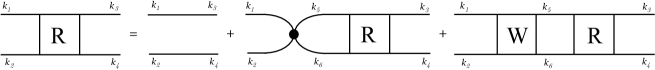
Figure 1: The Bethe-Salpeter equation for the response function $R$ of the many-body system in diagrammatic representation. The solid lines with arrows denote single-quasiparticle propagators. The integral part is divided into two terms, the small black circle represents the static effective interaction $\tilde{V}$ and the energy-dependent block $W(\omega)$ contains the dynamic contributions induced by the coupling to phonons.

The response of finite Fermi-systems with even particle number to an external perturbation is quantified by the response function which describes the propagation of the two-quasiparticles in the medium. The exact propagator includes, ideally, all possible kinds of the in-medium interaction between two arbitrary quasiparticles and contains all the information about the Fermi system that can be, in principle, extracted by various experimental probes whose interaction with the system can be represented by a single-quasiparticle operator and can be taken into account in the first order.

The response function $R$ is conventionally described by the Bethe-Salpeter equation (BSE). The general form of this equation

$$R(14,23)=G(1,3)G(4,2)-$$

$$-i\sum\limits_{5678}G(1,5)G(6,2)U(58,67)R(74,83),$$ (1)

involves the one-nucleon Green’s function (propagator) $G(1,2)$ in the nuclear medium and the effective nucleon-nucleon interaction $U(14,23)$. To include pairing correlations we use the formalism of the extended (doubled) space of the single-particle states described in Ref. LRT.08 . So, the number indices $1,2,...$ include all single-quasiparticle variables in an arbitrary representation in this doubled space and time. Respectively, the summation over the number indices implies an integration over the time variables. If $G$ is the exact single-quasiparticle Green’s function, $U$ is the amplitude of the effective interaction irreducible in the $ph$-channel. This amplitude is determined as a variational derivative of the nucleonic self-energy $\Sigma$ with respect to the exact single-quasiparticle Green’s function:

$$U(14,23)=i\frac{\delta\Sigma(4,3)}{\delta G(2,1)}.$$ (2)

Similar to Refs. Tse.07 ; LRT.08 , we decompose both the single-quasiparticle self-energy $\Sigma$ and the irreducible effective interaction $U$ into static ${\tilde{\Sigma}},\tilde{V}$ and time-dependent $\Sigma^{(e)},U^{(e)}$ parts as

$$\Sigma={\tilde{\Sigma}}+\Sigma^{(e)}$$ (3)

$$U={\tilde{V}}+U^{(e)}.$$ (4)

Accordingly, we introduce the uncorrelated response ${\tilde{R}}^{(0)}(14,23)={\tilde{G}}(1,3){\tilde{G}}(4,2)$, where ${\tilde{G}}(1,2)$ are the single-quasiparticle mean-field Green functions in the absence of the term $\Sigma^{(e)}$ in the self-energy. Then, it can be shown that the BSE (1) takes the form:

$$R(14,23)={\tilde{G}}(1,3){\tilde{G}}(4,2)-$$

$$-i\sum\limits_{5678}{\tilde{G}}(1,5){\tilde{G}}(6,2)V(58,67)R(74,83),$$ (5)

where $V$ is the new effective interaction amplitude which is specified below. The well-known quasiparticle random phase approximation (QRPA) including its relativistic version (RQRPA) corresponds to the case of $V\approx{\tilde{V}}$ neglecting the time-dependent term $U^{(e)}$. More precisely, in the (R)QRPA the time-dependent term is included in a static approximation by adjusting the parameters of the effective interaction $\tilde{V}$ to ground state properties of nuclei such as masses and radii. In the self-consistent (R)QRPA the static effective interaction is nothing but the second variational derivative of the covariant energy density functional (CEDF) $E[{\cal R}]$ with respect to the density matrix $\cal R$ VALR.05 :

$${\tilde{V}}(14,23)=\frac{2\delta^{2}E[{\cal R}]}{\delta{\cal R}(2,1)\delta{\cal R}(3,4)}.$$ (6)

In the approaches beyond the QRPA both static and time-dependent terms are contained in the residual interactions. In medium-mass and heavy nuclei vibrational and rotational modes emerge as collective degrees of freedom which are strongly coupled to the single-particle ones. The coupling to low-lying vibrations is known already for decades BM.75 as a very important mechanism of the formation of nuclear excited states and serves as a foundation for the so-called (quasi)particle-phonon coupling model. Implementations of this concept on the base of the modern density functionals have been extensively elaborated in non-relativistic CB.01 ; TSG.07 ; TSK.09 ; CSB.10 ; NCBBM.12 and relativistic LRT.08 ; LRT.10 ; LA.11 ; L.12 ; MLVR.12 frameworks.

In the present work we consider the quasiparticle-phonon coupling model for the time-dependent part of the nucleonic self-energy $\Sigma^{(e)}$ and the effective interaction $U^{(e)}$. We consider the BSE (5) in the time blocking approximation, first proposed in Ref. Tse.07 for superfluid Fermi systems and elaborated in detail in Ref. LRT.08 for the relativistic framework. This approximation allows an exact summation of a selected class of Feynman’s diagrams which give the leading contribution of the quasiparticle-phonon coupling effects. To apply this method it is convenient to write the BSE (5) in the representation in which the mean-field Green function $\tilde{G}$ is diagonal. In our case (see Ref. LRT.08 for more details) this representation is given by the set of the eigenfunctions $|\psi_{k}^{(\eta)}\rangle$ of the Relativistic Hartree-Bogoliubov (RHB) Hamiltonian $\mathcal{H}_{RHB}$ satisfying the equations KuR.91 :

$$\mathcal{H}_{RHB}|\psi_{k}^{(\eta)}\rangle=\eta E_{k}|\psi_{k}^{(\eta)}\rangle,\ \ \ \ {\cal H}_{RHB}=2\frac{\delta E[{\cal R}]}{\delta{\cal R}},$$ (7)

where $E_{k}>0$, the index $k$ stands for the set of the single-particle quantum numbers including states in the Dirac sea, and the index $\eta=\pm 1$ labels positive- and negative-frequency solutions of Eq. (7) in the doubled quasiparticle space. The eigenfunctions $|\psi_{k}^{(\eta)}\rangle$ are 8-dimensional Bogoliubov-Dirac spinors of the following structure:

$$|\psi_{k}^{(+)}(\mbox{\boldmath$r$})\rangle=\left(\begin{array}[c]{c}U_{k}(\mbox{\boldmath$r$})\\ V_{k}(\mbox{\boldmath$r$})\end{array}\right),\ \ \ \ |\psi_{k}^{(-)}(\mbox{\boldmath$r$})\rangle=\left(\begin{array}[c]{c}V_{k}^{\ast}(\mbox{\boldmath$r$})\\ U_{k}^{\ast}(\mbox{\boldmath$r$})\end{array}\right).$$ (8)

Within the time blocking approximation mentioned above and after performing a Fourier transformation to the energy domain, the BSE (5) for the spectral representation of the nuclear response function $R(\omega)$ in the basis $\{|\psi_{k}^{(\eta)}\rangle\}$ reads:

$$R_{k_{1}k_{4},k_{2}k_{3}}^{\eta\eta^{\prime}}(\omega)=\tilde{R}_{k_{1}k_{2}}^{(0)\eta}(\omega)\delta_{k_{1}k_{3}}\delta_{k_{2}k_{4}}\delta^{\eta\eta^{\prime}}+$$

$$+\tilde{R}_{k_{1}k_{2}}^{(0)\eta}(\omega)\sum\limits_{k_{5}k_{6}\eta^{\prime\prime}}{V}_{k_{1}k_{6},k_{2}k_{5}}^{\eta\eta^{\prime\prime}}(\omega)R_{k_{5}k_{4},k_{6}k_{3}}^{\eta^{\prime\prime}\eta^{\prime}}(\omega).$$ (9)

The quantity ${\tilde{R}}^{(0)}$

$${\tilde{R}}^{(0)\eta}_{k_{1}k_{2}}(\omega)=\frac{1}{\eta\omega-E_{k_{1}}-E_{k_{2}}}$$ (10)

describes the free propagation of two quasiparticles with their Bogoliubov’s energies $E_{k_{1}}$ and $E_{k_{2}}$ in the relativistic mean field. The interaction amplitude of Eq. (9) contains both static $\tilde{V}$ and dynamical (frequency-dependent) $W(\omega)$ parts (which will be specified below) and reads:

$${V}_{k_{1}k_{4},k_{2}k_{3}}^{\eta\eta^{\prime}}(\omega)=\tilde{V}_{k_{1}k_{4},k_{2}k_{3}}^{\eta\eta^{\prime}}+{W}_{k_{1}k_{4},k_{2}k_{3}}^{\eta\eta^{\prime}}(\omega),$$

$${W}_{k_{1}k_{4},k_{2}k_{3}}^{\eta\eta^{\prime}}(\omega)=\Bigl{[}\Phi_{k_{1}k_{4},k_{2}k_{3}}^{\eta}(\omega)-\Phi_{k_{1}k_{4},k_{2}k_{3}}^{\eta}(0)\Bigr{]}\delta^{\eta\eta^{\prime}}.$$ (11)

The diagrammatic representation of the Eq. (9) is given in Fig. 1. Notice here, that in outward appearance this diagrammatic equation written, as in Ref. LRT.08 , for the system with pairing correlations has the same form as that for the normal (non-superfluid) system. The formal similarity of the equations for the normal and superfluid systems is achieved by the use of the representation of the basis functions $|\psi_{k}^{(\eta)}\rangle$ satisfying Eq. (7). This basis is a counterpart of the particle-hole basis of the conventional RPA in which the (Q)RPA equations have the most simple and compact form. In the representation of the functions $|\psi_{k}^{(\eta)}\rangle$ the generalized superfluid mean-field Green function $\tilde{G}$ (often called Gor’kov-Green’s function) has a diagonal form and describes the propagation of the quasiparticle with the fixed energy. In this diagonal representation the directions of the arrows in the fermion lines of the diagrams (of the type shown in Fig. 1) label the positive- or the negative-frequency components of the functions $\tilde{G}$. It should be noted that the so-called backward-going diagrams corresponding to the ground-state correlations in the RQRPA are not shown in Fig. 1 though they are included in Eq. (9).

If we come back to the coordinate representation using Eqs. (8) we get the non-diagonal Green function $\tilde{G}$ for the quasiparticle which has no definite energy. In the diagrammatic language this Green function can be represented by the 2$\times$2 block matrix shown in Fig. 2. The matrix elements of this matrix are the normal and anomalous Green functions of the conventional Gor’kov theory. In this representation it is clearly seen that the difference between the normal and the superfluid systems is that in the latter case all the quantities acquire additional components in the doubled quasiparticle space. Obviously, all these components are incorporated in the representation of the functions $|\psi_{k}^{(\eta)}\rangle$ in the implicit form. On the other hand, the use of the basis $\{|\psi_{k}^{(\eta)}\rangle\}$ allow us to reduce by a factor of 2 the dimension of the system of the equations for the response function. This property of the diagonal representation of the superfluid mean-field Green functions has been already utilized in our previous papers (see, e.g., Refs. LRT.08 ; Tse.07 ; LT.07 ) but not discussed in detail.

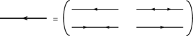
Figure 2: The 4-component Green’s function in the diagrammatic representation.

In the present work, as in Refs. LRT.08 ; LRTL.09 , the static amplitude $\tilde{V}$ of Eq. (6) is derived from the covariant energy density functional $E[{\cal R}]$ with the parameter set NL3 NL3 as a one-meson exchange interaction with a non-linear self-coupling between the mesons. As in Ref. LRT.08 , pairing correlations are introduced into the relativistic energy density functional as an independently parameterized term in the form of a monopole interaction with constant $G$ matrix elements. In the BSE the set of the quasiparticle variables is doubled and therefore we have a formulation in terms of 4-component Green’s functions, as explained above. In the 2q$\otimes$phonon version of the RQTBA the frequency-dependent residual interaction $\Phi(\omega)$ is related to the quasiparticle-phonon coupling self-energy by the consistency condition and calculated within the quasiparticle time blocking approximation. This approximation means that, due to the time projection in the integral part of the BSE, the two-body propagation through states with a more complicated structure than 2q$\otimes$phonon is blocked Tse.07 . The diagrammatic representation of the 2q$\otimes$phonon amplitude is shown in the upper line of Fig. 3.

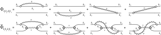
Figure 3: The correspondence between the 2q$\otimes$phonon amplitude $\Phi$ of the conventional phonon coupling model and the two-phonon amplitude $\bar{\Phi}$ of the two-phonon model in a diagrammatic representation. Solid lines with arrows and Latin indices denote the single-quasiparticle nucleonic propagators, wavy curves with Greek indices show the phonon propagators, empty circles represent phonon vertices, and grey circles with the two attached nucleonic lines denote the RQRPA transition densities (see text).

In order to go a step further, notice, that in the time blocking approximation the energy-dependent resonant part of the two-quasiparticle amplitude $\Phi(\omega)$ can be factorized in a special way Tse.07 . Namely, the two-quasiparticle intermediate propagator, appearing as the two uncorrelated quasiparticle lines between the phonon emission and absorption vertices in the upper part of the Fig. 3, can be extracted. Thus, in the relativistic QTBA the amplitude $\Phi(\omega)$ takes the following form:

$$\Phi^{\eta}_{k_{1}k_{4},k_{2}k_{3}}(\omega)=\sum_{k_{5}k_{6},\mu}\zeta^{\,\mu\eta}_{k_{1}k_{2};k_{5}k_{6}}\,\tilde{R}^{(0)\eta}_{k_{5}k_{6}}(\omega-\eta\,\Omega_{\mu})\,\zeta^{\,\mu\eta*}_{\,k_{3}k_{4};k_{5}k_{6}}\,,$$ (12)

where $\tilde{R}^{(0)\eta}_{k_{5}k_{6}}(\omega-\eta\,\Omega_{\mu})$ are the matrix elements of the two-quasiparticle propagator in the mean field with the frequency shifted forward or backward by the phonon energy $\Omega_{\mu}$,

$$\zeta^{\,\mu(+)}_{\,k_{1}k_{2};k_{5}k_{6}}=\delta^{\vphantom{(+)}}_{k_{1}k_{5}}\,\gamma^{(-)}_{\mu;k_{6}k_{2}}-\gamma^{(+)}_{\mu;k_{1}k_{5}}\delta^{\vphantom{(+)}}_{k_{6}k_{2}},$$

$$\zeta^{\,\mu(-)}_{\,k_{1}k_{2};k_{5}k_{6}}=\delta^{\vphantom{(+)}}_{k_{5}k_{1}}\,\gamma^{(+)\ast}_{\mu;k_{2}k_{6}}-\gamma^{(-)\ast}_{\mu;k_{5}k_{1}}\delta^{\vphantom{(+)}}_{k_{2}k_{6}},$$ (13)

so that

$$\zeta^{\,\mu(-)}_{\,k_{1}k_{2};k_{5}k_{6}}=-\zeta^{\,\mu(+)\ast}_{\,k_{2}k_{1};k_{6}k_{5}}.$$ (14)

In Eq. (13) and below we use a shorthand notation for the phonon amplitudes involved in the present work:

$$\gamma^{\eta}_{\mu;k_{1}k_{2}}=\gamma^{\eta_{1}\eta_{2}}_{\mu;k_{1}k_{2}}\delta_{\eta\eta_{1}}\delta_{\eta\eta_{2}},\ \ \ \ \eta=(\pm)$$ (15)

where the vertices ${\gamma}_{\mu;k_{1}k_{2}}^{\eta_{1}\eta_{2}}$ determine the coupling of the quasiparticles to the collective vibrational state (phonon) $\mu$. In the conventional version of the quasiparticle-vibration coupling model these vertices are derived from the corresponding RQRPA transition densities $\mathcal{R}_{\mu}$ and the static effective interaction as

$$\gamma_{\mu;k_{1}k_{2}}^{\eta_{1}\eta_{2}}=\sum\limits_{k_{3}k_{4}}\sum\limits_{\eta}\tilde{V}_{k_{1}k_{4},k_{2}k_{3}}^{\eta_{1},-\eta_{,}\eta_{2},\eta}\mathcal{R}_{\mu;k_{3}k_{4}}^{\eta}$$ (16)

where $\tilde{V}_{k_{1}k_{4},k_{2}k_{3}}^{\eta_{1}\eta_{4},\eta_{2}\eta_{3}}$ is the matrix element of the amplitude $\tilde{V}$ of Eq. (6) in the basis $\{|\psi_{k}^{(\eta)}\rangle\}$. The matrix elements of the phonon transition densities are calculated, in a first approximation, within the relativistic quasiparticle random phase approximation PRN.03 . In the Dirac-Hartree-BCS basis $\{|\psi_{k}^{(\eta)}\rangle\}$ it has the following form:

$$\mathcal{R}_{\mu;k_{1}k_{2}}^{\eta}={\tilde{R}}_{k_{1}k_{2}}^{(0)\eta}(\Omega_{\mu})\sum\limits_{k_{3}k_{4}}\sum\limits_{\eta^{\prime}}\tilde{V}_{k_{1}k_{4},k_{2}k_{3}}^{\eta\eta^{\prime}}\mathcal{R}_{\mu;k_{3}k_{4}}^{\eta^{\prime}},$$ (17)

where $\tilde{V}_{k_{1}k_{4},k_{2}k_{3}}^{\eta\eta^{\prime}}=\tilde{V}_{k_{1}k_{4},k_{2}k_{3}}^{\eta,-\eta^{\prime},-\eta,\eta^{\prime}}$. This means that we cut out the components of the tensors in the quasiparticle space, which are relevant for the particle-hole channel.

In the graphic expression of the amplitude (12) in the upper line of the Fig. 3 the uncorrelated propagator $\tilde{R}^{(0)\eta}_{k_{1}k_{2}}$ is represented by the two straight nucleonic lines between the circles denoting emission and absorption of the phonon by a single quasiparticle with amplitudes $\gamma^{\eta_{1}\eta_{2}}_{\mu;k_{1}k_{2}}$. The approach to the amplitude $\Phi(\omega)$ expressed by the Eq. (12) represents a version of first-order perturbation theory compared to RQRPA and the amplitude $\Phi(\omega)$ of Eq. (11) is the first-order correction to the effective interaction ${\tilde{V}}$, because the dimensionless matrix elements of the phonon vertices are such that $\gamma^{\eta_{1}\eta_{2}}_{\mu;k_{1}k_{2}}/\Omega_{\mu}\ll 1$ in most of the physical cases. The phonon-coupling term $\Phi$ generates fragmentation of nuclear excited states. For giant resonances this fragmentation is the source of the spreading width and in the low-energy region below the neutron threshold this term is responsible almost solely for the appearing strength. In the relativistic framework, this was confirmed and extensively studied LRT.08 ; LRTL.09 and verified by comparison to experimental data E.10 ; M.12 . However, a comparison with high-resolution experiments on the dipole strength below the neutron threshold has revealed that although the total strength and some gross features of the strength are reproduced well, the fine features are sensitive to the truncation of the configuration space by 2q$\otimes$phonon configurations and further extensions of the method are due. The first possible extension of this model uses the idea proposed in Ref. Tse.07 . It is based on the factorization of Eq. (12): the uncorrelated propagator ${\tilde{R}}^{(0)\eta}$ in Eq. (12) is replaced by the positive- ($\eta=+1$) or the negative- ($\eta=-1$) frequency part of a correlated one which, in first order approximation, is the antisymmetrized RQRPA propagator $R^{(RQRPA)\eta}$. Instead of the amplitude $\Phi$, we have the new amplitude $\bar{\Phi}$:

$${\bar{\Phi}}^{\eta}_{k_{1}k_{4},k_{2}k_{3}}(\omega)=\frac{1}{2}\sum_{k_{5}k_{6},k_{5^{\prime}}k_{6^{\prime}}\mu}\zeta^{\,\mu\eta}_{k_{1}k_{2};k_{5}k_{6}}\,$$ (18)

$$\times R^{(RQRPA)\eta}_{k_{5}k_{6^{\prime}},k_{6}k_{5^{\prime}}}(\omega-\eta\,\Omega_{\mu})\,\zeta^{\,\mu\eta*}_{\,k_{3}k_{4};k_{5^{\prime}}k_{6^{\prime}}}.$$

The factor $1/2$ in Eq. (18) appears due to the antisymmetrization of Eq. (12) as was explained in Ref. Tse.07 . This antisymmetrization implies that the following equations are fulfilled

$$R^{(RQRPA)\eta}_{k_{1}k_{4},k_{2}k_{3}}(\omega) = -R^{(RQRPA)\eta}_{k_{2}k_{4},k_{1}k_{3}}(\omega)$$ (19)

$$= -R^{(RQRPA)\eta}_{k_{1}k_{3},k_{2}k_{4}}(\omega)$$

which are not valid for the uncorrelated propagator ${\tilde{R}}^{(0)\eta}$. By this substitution, we introduce RQRPA correlations into the intermediate two-quasiparticle propagators, i.e., in diagrammatic language, we perform the operation shown in Fig. 4.

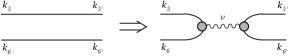
Figure 4: Replacement of the uncorrelated two-nucleon propagator by the correlated one. Grey circles with the two attached nucleonic lines and wavy curve denote the RQRPA transition densities and the phonon propagator, respectively.

Thus, two-phonon configurations appear in the amplitude $\Phi(\omega)$ as it is clear from the diagrammatic representation of the new amplitude $\bar{\Phi}$ shown in the bottom line of Fig. 3. The analytic expression of this amplitude reads:

$${\bar{\Phi}}^{\eta}_{k_{1}k_{4},k_{2}k_{3}}(\omega)=\frac{1}{2}\sum_{\mu,\nu}\frac{{\bar{\zeta}}^{\,\eta}_{\,\mu\nu;k_{1}k_{2}}\,{\bar{\zeta}}^{\,\eta*}_{\,\mu\nu;k_{3}k_{4}}}{\eta\,\omega-\Omega_{\mu}-\Omega_{\nu}}\,,$$ (20)

where

$${\bar{\zeta}}^{\,(+)}_{\,\mu\nu;k_{1}k_{2}} = \sum_{k_{6}}{\cal R}^{(+)}_{\,\nu;k_{1}k_{6}}\,\gamma^{(-)}_{\,\mu;k_{6}k_{2}}\,-\sum_{k_{5}}\gamma^{(+)}_{\,\mu;k_{1}k_{5}}\,{\cal R}^{(+)}_{\,\nu;k_{5}k_{2}}$$

$${\bar{\zeta}}^{\,(-)}_{\,\mu\nu;k_{1}k_{2}} = {\bar{\zeta}}^{\,(+)\ast}_{\,\mu\nu;k_{2}k_{1}},$$ (21)

and ${\cal R}^{\eta}_{\,\nu;k_{1}k_{2}}$ are the matrix elements of the RQRPA transition densities defined in Eq. (17) and corresponding to grey circles together with two nucleonic lines in Fig. 3. One can show that in the limit of vanishing static interaction $\tilde{V}$ between the two intermediate quasiparticles Eq. (20) transforms to the antisymmetrized Eq. (12) of the original (R)QTBA. As in conventional (R)QTBA, the elimination of double counting effects in the phonon coupling is performed by the subtraction of the static contribution of the amplitude ${\bar{\Phi}}$ from the residual interaction in Eq. (11), since the parameters of the CEDF have been adjusted to experimental data for ground states and include therefore already essential phonon contributions to the ground state. Therefore, the BSE in the two-phonon model has the same form as Eq. (9), but it contains the amplitude $\bar{\Phi}$ instead of $\Phi$.

The calculations are performed in the following four steps: (i) The RHB equation (7) is solved to determine the single-quasiparticle energies and wave functions. These wave functions serve as a working basis for the subsequent calculations. (ii) The phonon frequencies, their coupling vertices $\gamma^{\eta}$ and the transition densities ${\cal R}^{\eta}$ are calculated within the self-consistent RQRPA using the static residual interaction $\tilde{V}$. (iii) The BSE for the correlated propagator $R^{(e)}(\omega)$

$$R^{(e)\eta}_{k_{1}k_{4},k_{2}k_{3}}(\omega)={\tilde{R}}^{(0)\eta}_{k_{1}k_{2}}(\omega)\delta_{k_{1}k_{3}}\delta_{k_{2}k_{4}}+$$

$$+{\tilde{R}}^{(0)\eta}_{k_{1}k_{2}}(\omega)\sum\limits_{k_{5}k_{6}}\bigl{[}{\bar{\Phi}}^{\eta}_{k_{1}k_{6},k_{2}k_{5}}(\omega)-{\bar{\Phi}}^{\eta}_{k_{1}k_{6},k_{2}k_{5}}(0)\bigr{]}\times$$

$$\times R^{(e)\eta}_{k_{5}k_{4},k_{6}k_{3}}(\omega),$$ (22)

is solved in the Dirac-Hartree-BCS basis; (iv) the BSE for the full response function $R(\omega)$

$$R_{k_{1}k_{4},k_{2}k_{3}}^{\eta\eta^{\prime}}(\omega) = R^{(e)\eta}_{k_{1}k_{4},k_{2}k_{3}}(\omega)\delta^{\eta\eta^{\prime}}$$ (23)

$$+ \sum\limits_{k_{5}k_{6}k_{7}k_{8}}R^{(e)\eta}_{k_{1}k_{6},k_{2}k_{5}}(\omega)$$

$$\times \sum\limits_{\eta^{\prime\prime}}{\tilde{V}}_{k_{5}k_{8},k_{6}k_{7}}^{\eta\eta^{\prime\prime}}R_{k_{7}k_{4},k_{8}k_{3}}^{\eta^{\prime\prime}\eta^{\prime}}(\omega)$$

where

$$R_{k_{1}k_{4},k_{2}k_{3}}^{\eta\eta^{\prime}}(\omega) = R_{k_{1}k_{4},k_{2}k_{3}}^{\eta,-\eta^{\prime},-\eta,\eta^{\prime}}(\omega),$$

$${\tilde{V}}_{k_{1}k_{4},k_{2}k_{3}}^{\eta\eta^{\prime}} = {\tilde{V}}_{k_{1}k_{4},k_{2}k_{3}}^{\eta,-\eta^{\prime},-\eta,\eta^{\prime}},$$ (24)

is solved in the momentum-channel representation which is especially convenient because of the structure of the one-boson exchange interaction. The details are given below.

III Bethe-Salpeter equation in the coupled form

For the spherically symmetric case Eq. (22) is formulated in terms of the reduced matrix elements with the transferred angular momentum $J$, i.e. in the so-called coupled form, as follows:

$$R_{(k_{1}k_{4},k_{2}k_{3})}^{(e)J,\eta}(\omega) = {\tilde{R}}^{(s)J,\eta}_{(k_{1}k_{4},k_{2}k_{3})}(\omega)+$$

$$+{\tilde{R}}^{(0)\eta}_{(k_{1}k_{2})}(\omega)\sum\limits_{(k_{6}\leq k_{5})}\Bigl{[}{\bar{\Phi}}_{(k_{1}k_{6},k_{2}k_{5})}^{(s)J,\eta}(\omega) - {\bar{\Phi}}_{(k_{1}k_{6},k_{2}k_{5})}^{(s)J,\eta}(0)\Bigr{]}\times$$ (25)

$$\times R_{(k_{5}k_{4},k_{6}k_{3})}^{(e)J,\eta}(\omega).$$

The index ”(s)” implies here that the corresponding matrix elements are symmetrized with respect to one non-conjugated and one conjugated quasiparticle index. Such a symmetrization allows a shortened summation in the integral part of the Eq. (25) and simplifies, to some extent, the numerical calculations. The symmetrized matrix elements of the mean field propagator ${\tilde{R}}^{(s)}$ and of the two quasiparticles-phonon coupling amplitude $\Phi^{(s)}$ have the following form:

$${\tilde{R}}^{(s)J,\eta}_{(k_{1}k_{4},k_{2}k_{3})}(\omega)={\tilde{R}}^{(0)\eta}_{(k_{1}k_{2})}(\omega)\times$$

$$\times\bigl{[}\delta_{(k_{1}k_{3})}\delta_{(k_{2}k_{4})}+(-)^{\phi_{12}}\delta_{(k_{1}k_{4})}\delta_{(k_{2}k_{3})}\bigr{]},$$ (26)

$${\bar{\Phi}}^{(s)J,\eta}_{(k_{1}k_{4},k_{2}k_{3})}(\omega)=\frac{1}{1+\delta_{(k_{3}k_{4})}}\times$$

$$\times\Bigl{[}{\bar{\Phi}}^{J,\eta}_{(k_{1}k_{4},k_{2}k_{3})}(\omega)+(-)^{\phi_{12}}{\bar{\Phi}}^{J,\eta}_{(k_{2}k_{4},k_{1}k_{3})}(\omega)\Bigr{]},$$ (27)

where $\phi_{12}=J+l_{1}-l_{2}+j_{1}-j_{2}$. The reduced matrix elements of the phonon coupling amplitudes for the two-phonon model can be expressed as:

$${\bar{\Phi}}^{J,\eta}_{(k_{1}k_{4},k_{2}k_{3})}(\omega)=\frac{1}{2(2J+1)}\sum\limits_{(\mu,\nu)}\frac{{\bar{\zeta}}^{\eta}_{(\mu\nu;k_{1}k_{2})}{\bar{\zeta}}^{\eta\ast}_{(\mu\nu;k_{3}k_{4})}}{\eta\omega-\omega_{\mu}-\omega_{\nu}}\,,$$ (28)

$${\bar{\zeta}}^{(+)}_{(\mu\nu;k_{1}k_{2})}=(-1)^{j_{1}+j_{2}}\times$$

$$\times\Bigl{[}\sum\limits_{(k_{6})}\gamma_{({\mu};k_{6}k_{2})}^{(-)}{\cal R}_{({\nu};k_{1}k_{6})}^{(+)}\left\{\begin{array}[c]{ccc}J_{\mu}&J_{\nu}&J\\ j_{1}&j_{2}&j_{6}\end{array}\right\}$$ (31)

$$-(-1)^{J_{\mu}+J_{\nu}+J}\sum\limits_{(k_{5})}\gamma_{(\mu;k_{1}k_{5})}^{(+)}{\cal R}_{(\nu;k_{5}k_{2})}^{(+)}\left\{\begin{array}[c]{ccc}J_{\nu}&J_{\mu}&J\\ j_{1}&j_{2}&j_{5}\end{array}\right\}\Bigr{]},$$ (34)

$${\bar{\zeta}}^{(-)}_{(\mu\nu;k_{1}k_{2})}=(-1)^{J_{\mu}+J_{\nu}+J}{\bar{\zeta}}^{(+)}_{(\mu\nu;k_{2}k_{1})}.$$ (35)

Then, the BSE for the full response function $R(\omega)$

$$R_{(k_{1}k_{4},k_{2}k_{3})}^{J,\eta\eta^{\prime}}(\omega)=R_{(k_{1}k_{4},k_{2}k_{3})}^{(e)J,\eta}(\omega)\delta^{\eta\eta^{\prime}}+\sum\limits_{(k_{6}\leq k_{5})}\times$$

$$\times\sum\limits_{(k_{8}\leq k_{7})\eta^{\prime\prime}}R_{(k_{1}k_{6},k_{2}k_{5})}^{(e)J,\eta}(\omega){\tilde{V}}^{J,\eta\eta^{\prime\prime}}_{(k_{5}k_{8},k_{7}k_{6})}R_{(k_{7}k_{4},k_{8}k_{3})}^{J,\eta^{\prime\prime}\eta^{\prime}}(\omega)$$

(36)

is solved in both Dirac-Hartree-BCS and momentum-channel representations. This latter representation is especially convenient for numerical solution of the BSE with the static effective interaction $\tilde{V}$ of the one-boson exchange type. The expressions for the reduced matrix elements ${\tilde{V}}^{J,\eta\eta^{\prime\prime}}_{(k_{5}k_{8},k_{7}k_{6})}$ of this interaction in doubled quasiparticle space and further details are given in the Appendix C of Ref. LRT.08 . The resulting linear response function $R(\omega)$ contains all the information on the nuclear response to external one-body operators. To describe the observed spectrum of a nucleus excited by a sufficiently weak external field $P$ as, for instance, an electromagnetic field, one has to make a double convolution of the response function with this field. The reduced matrix elements of the external field operator have the following general coupled form:

$$P_{(k_{1}k_{2})}^{(p)J,\eta}=\sum\limits_{LS}\frac{\delta_{\eta,1}+(-1)^{S}\delta_{\eta,-1}}{\sqrt{1+\delta_{(k_{1}k_{2})}}}\eta^{S}_{(k_{1}k_{2})}\times$$

$$\times\langle(k_{1})\parallel P^{(p)J}_{LS}\parallel(k_{2})\rangle,$$ (37)

where the index $(p)$ contains all possible quantum numbers other than those concretized here. The factors $\eta^{S}_{(k_{1}k_{2})}$ are the conventional factors RS.80 determined by combinations of the quasiparticle occupation numbers $u_{k},v_{k}$:

$$\eta_{(k_{1}k_{2})}^{S}=\frac{1}{\sqrt{1+\delta_{(k_{1}k_{2})}}}\Bigl{(}u_{k_{1}}v_{k_{2}}+(-1)^{S}v_{k_{1}}u_{k_{2}}\Bigr{)}$$ (38)

obtained as a solution of Eq. (7). Such combinations arise due to symmetrization in the integral part of the Eq. (36), which enables one to take each $2q$-pair into account only once because of the symmetry properties of the reduced matrix elements ${\tilde{V}}^{J,\eta\eta^{\prime\prime}}_{(k_{5}k_{8},k_{7}k_{6})}$.

The double convolution of the response function with the external field operator defines the quantity called nuclear polarizability:

$$\Pi_{P}(\omega) = \sum\limits_{(k_{2}\leq k_{1})\eta}\sum\limits_{(k_{4}\leq k_{3})\eta^{\prime}}P_{(k_{1}k_{2})}^{(p)J,\eta\ast}$$ (39)

$$\times R_{(k_{1}k_{4},k_{2}k_{3})}^{J,\eta\eta^{\prime}}(\omega)P_{(k_{3}k_{4})}^{(p)J,\eta^{\prime}}$$

which determines the microscopic strength function $S(E)$ as:

$$S(E)=-\frac{1}{\pi}\lim\limits_{\Delta\to+0}Im\Pi_{P}(E+i\Delta).$$ (40)

In the calculations a finite imaginary part $\Delta$ of the energy variable is introduced for convenience in order to obtain a smoothed envelope of the spectrum. This parameter introduces an additional artificial width for each excitation. This width emulates effectively contributions from configurations higher than 4q and the coupling to the continuum, which are not taken into account explicitly in our approach.

IV Results and discussion

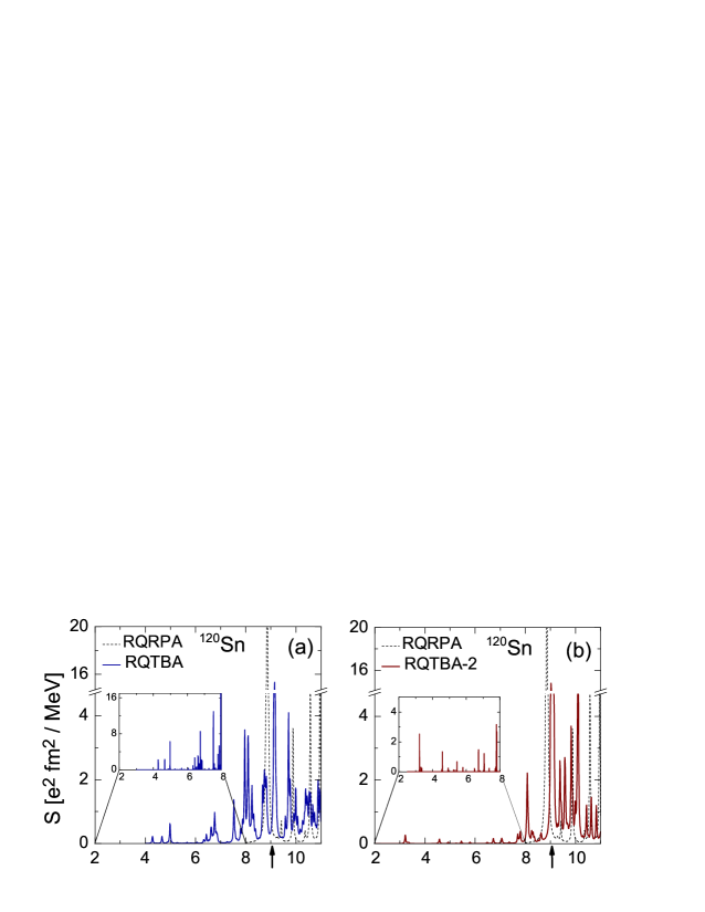
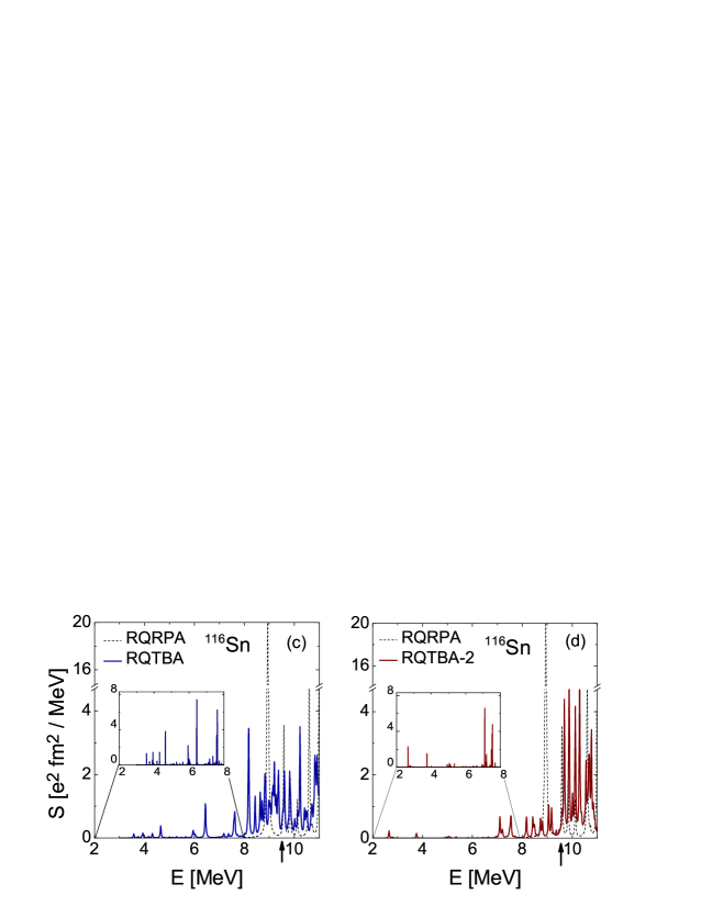
Figure 5: Low-lying dipole spectra of ^116,120Sn calculated within RQRPA (dashed curves), RQTBA (blue solid curve, panels (a,c)) and RQTBA-2 (red solid curve, panels (b,d)). A finite smearing parameter $\Delta$ = 20 keV has been used in the calculations. The inserts show the zoomed pictures of the spectra below 8 MeV with a smaller value $\Delta$ = 2 keV allowing to see all the states in this energy region. The arrows indicate the neutron thresholds.

To illustrate the effect of the two-phonon correlations on spectra of nuclear excitations, we consider the dipole response of tin and nickel isotopes in the energy region below the giant dipole resonance (GDR). Fig. 5 displays the electromagnetic dipole strength functions in ^116,120Sn calculated within conventional RQTBA LRT.08 and two-phonon RQTBA-2 presented here. The strength functions obtained in this way are compared with the original RQRPA strength function because both of them originate from RQRPA by different fragmentation mechanisms. The first observation is that the total strength $\sum B(E1)\uparrow$ below the neutron threshold is reduced in RQTBA-2. For example, for ¹¹⁶Sn we have 0.20 e² fm² below 8 MeV which agrees with 0.204(25) e² fm² obtained in the experiment of Ref. Gov.98 . For ¹²⁰Sn, if we include the relatively strong state at 8.08 MeV into the integration region, this quantity is 0.31 e² fm², in agreement with the results of the quasiparticle phonon model (QPM) of 0.289 e² fm² TLS.04 . One also notices that in both nuclei the major fraction of the RQRPA pygmy mode shown by the dashed curve is pushed up above the neutron threshold by the RQTBA-2 correlations.

Table 1: The energies, reduced transition probabilities and anharmonicities of the lowest 1^- states in ^{112,116,120,124}Sn isotopes calculated in the relativistic two-phonon model, compared to data of Refs. Pys.06 ; Bry.99 ; OEN.07 ; Gov.98 ; Oezel.phd and to QPM calculations of Ref. Pys.06 , see text for details.

		$\omega$(1${}^{-}_{1}$)	B(E1)$\uparrow$	$R_{\omega}$
		(MeV)	($10^{-3}$ e2 fm2)
	RQTBA-2	3.85	26.12	0.98
112Sn	QPM	3.24	1.6
	Exp. Pys.06	3.43	10.7(12)	0.95
	Exp. OEN.07	3.43	15.0(10)
	RQTBA-2	2.66	14.33	0.94
116Sn	QPM	3.35	8.2
	Exp. Bry.99	3.33	6.55(65)	0.94
	Exp. Gov.98 ; OEN.07	3.33	16.3(9)
	RQTBA-2	3.23	15.90	0.95
120Sn	QPM	3.32	7.2
	Exp. Bry.99	3.28	7.60(51)	0.92
	Exp. Oezel.phd	3.28	11.2(11)
	RQTBA-2	3.98	12.91	0.97
124Sn	QPM	3.57	3.5
	Exp. Bry.99	3.49	6.1(7)	0.93
	Exp. Gov.98 ; OEN.07	3.49	10.0(5)

The energies, the corresponding $B(E1)\uparrow$ values and the $R_{\omega}$ values defined as $R_{\omega}=\omega(1^{-}_{1})/\bigl{(}\omega(2^{+}_{1})+\omega(3^{-}_{1})\bigr{)}$ for the lowest 1^- states in the tin isotopes are listed in Table 1. The experimental energies, $B(E1)\uparrow$ and $R_{\omega}$ values are taken from Refs. Pys.06 ; Bry.99 ; OEN.07 ; Gov.98 ; Oezel.phd where they were extracted from photon scattering data. The results obtained within QPM are included for comparison. Notice, that the measurements with larger end point energies for the electron bremsstrahlung result in larger $B(E1)\uparrow$ values Gov.98 ; OEN.07 ; Oezel.phd . Fig. 6 shows the results obtained for the energies and reduced transition probabilities B(E1)$\uparrow$ in the chain of tin isotopes ^{112,116,120,124}Sn within the relativistic two-phonon model. The obtained results are compared to the same sets of data as in the Table 1. One can see that the RQTBA-2 results for the $1^{-}_{1}$ states in ^{112,116,120,124}Sn are in a better agreement to the data obtained with larger end point energies while the QPM results rather support another data set. For ^112,124Sn, however, the QPM transition probabilities are too small.

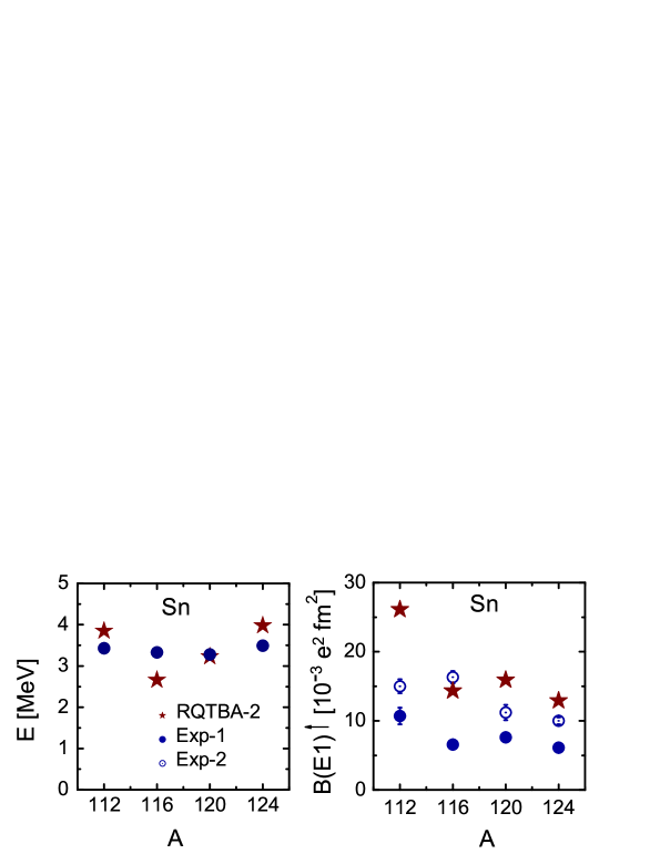
Figure 6: Energies and B(E1)$\uparrow$ values of the first $1^{-}$ states in the chain of tin isotopes ^{112,116,120,124}Sn obtained within the relativistic two-phonon model (stars), compared to data from Refs. Pys.06 ; Bry.99 ; Gov.98 (filled circles), and OEN.07 ; Oezel.phd (open circles).

In RQTBA-2, the position of the first 1^- state is basically defined by the sum of the energies of the lowest 2⁺ and 3^- phonons. From the Eq. (20) one can see that the amplitude $\bar{\Phi}(\omega)$ consists of the pole terms with the poles at the energies which are sums of the two phonon energies. Thus, the energy of the first 1^- state is approximately equal to the sum of the energies of the lowest 2⁺ and 3^- phonons with some relatively small negative correction introduced by the static residual interaction $\tilde{V}$. Similar conclusions follow from the analysis of the experimentally observed energies of the lowest $2^{+}$, $3^{-}$ and $1^{-}$ states, see a discussion in Ref. Bry.99 . The above mentioned correction is quantified by the value of $R_{\omega}$, whose deviation from unity characterizes the two-phonon anharmonicity, see Table 1. In particular, in ¹²⁰Sn the energies of the $2^{+}_{1}$ and $3^{-}_{1}$ phonons calculated within the RQRPA are obtained at 1.48 MeV and 1.90 MeV, respectively, and the 1${}^{-}_{1}$ state appears at 3.23 MeV in the two-phonon approach. Thus, the quality of description of the first $1^{-}$ two-phonon state is mainly determined by the quality of description provided by the RQRPA for the $2^{+}_{1}$ and $3^{-}_{1}$ phonons, namely, their energies and coupling vertices. In the cases of vibrational nuclei, these quantities are reasonably well described by the RQRPA, however, the description could be further improved by inclusion of correction beyond RQRPA. A relatively small anharmonicity allows an identification of the first experimentally observed $1^{-}$ state as a member of the $2^{+}_{1}\otimes 3^{-}_{1}$ quintuplet. Theoretically, we have shown that this state appears solely due to the inclusion of the two-phonon correlations and does not appear in the spectra calculated within the conventional RQTBA, although 2q$\otimes$phonon ”prototypes” of this two-phonon state are present in the RQTBA model space at higher energies. One can see that for the lowest $1^{-}$ state in the considered chain of even-even tin isotopes the obtained agreement of the RQTBA-2 results with the available data is very good in spite of the fact that this tiny structure at about 3 MeV originates by the splitting-out from the very strong RQRPA pygmy mode located at the neutron threshold, due to the two-phonon correlations included consistently without any adjustment procedures.

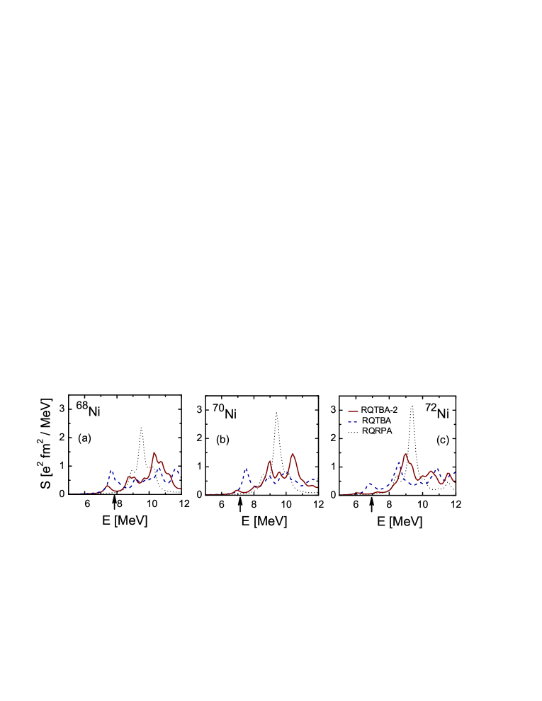
Figure 7: Low-lying dipole spectrum of ^68,70,72Ni calculated within the RQRPA (black dotted curves), RQTBA (blue dashed curves), and RQTBA-2 (red solid curves) with a smearing parameter of 200 keV. The arrows show the neutron thresholds.

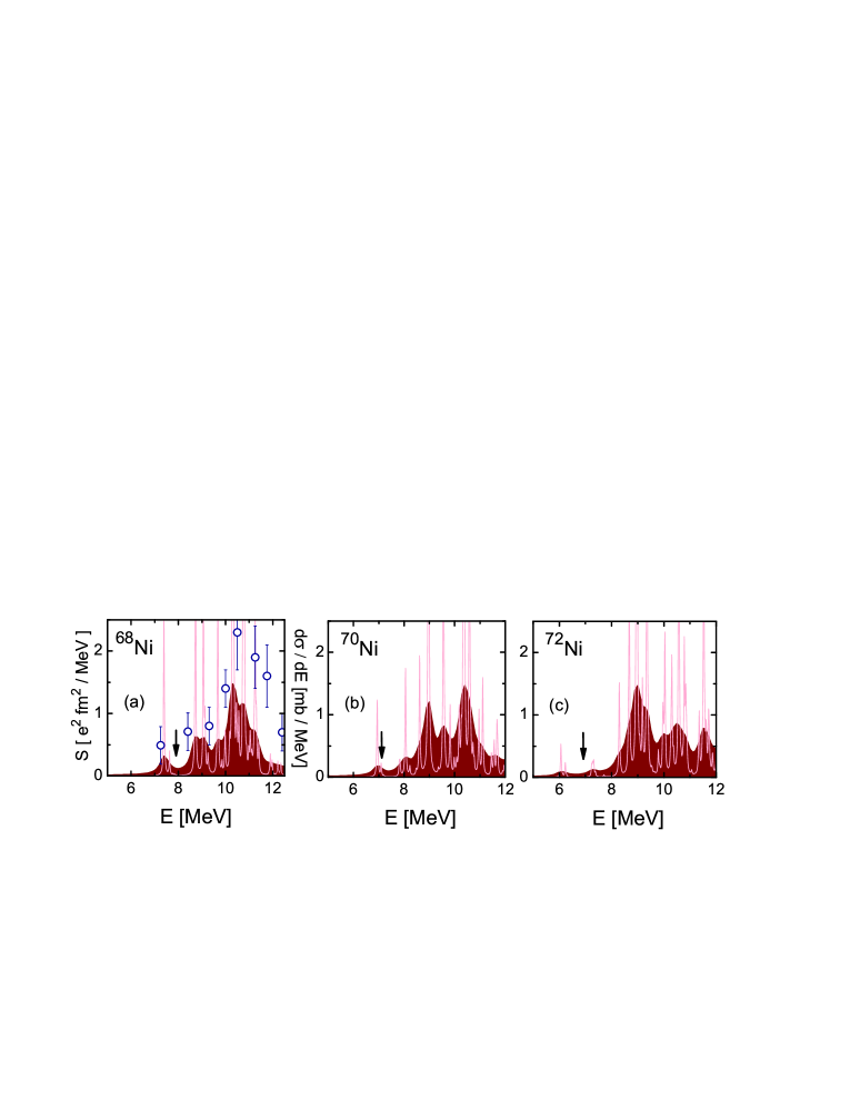
Figure 8: Low-lying dipole spectra of ^68,70,72Ni calculated within RQTBA-2 with a smearing parameter of 20 keV (thin curves, light pink) and 200 keV (filled area). Panel (a) contains also the data from Ref. WBC.09 (open circles, units on the right). The arrows show the neutron thresholds.

The low-lying electromagnetic dipole strengths in neutron rich ^68,70,72Ni isotopes are displayed in Figs. 7,8. Fig. 7 shows the RQTBA-2 strength functions compared to the RQTBA and the original RQRPA, and Fig. 8 shows the RQTBA-2 strength distributions calculated with different smearing parameters so that the fine structure of the strength can be analyzed. In contrast to the case of tin isotopes, in the considered Ni isotopes almost the whole pygmy dipole resonance is located above the neutron threshold. For all three isotopes we found a redistribution and weaker fragmentation of the low-lying strength in RQTBA-2 compared to the RQTBA calculations of Ref. LRTL.09 . The calculated strength distribution in ⁶⁸Ni has its maximum at 10.30 MeV and the total strength below 12 MeV is 2.73 e² fm², while the corresponding fraction of the energy weighted sum rule (EWSR) is 7.8% of the total integrated photoabsorption cross section and 11% of the Thomas-Reiche-Kuhn sum rule. These characteristics are in agreement with those extracted from the recent data reported in Ref. WBC.09 which are also included in Fig. 8. The data are given for the differential cross section, so that the shape of the measured distribution can be compared to the theoretical strength. The RQTBA-2 dipole strength distributions for the ^70,72Ni isotopes can be suggested as predictions for possible future measurements in these nuclei. One can see that with the increase of the neutron number the total strength increases and the centroid of the pygmy dipole resonance shifts toward lower energy, however, this evolution is very smooth within the considered isotopic chain. The reason is the occupation of the 1g_9/2 intruder orbit in the neutron subsystem, as it has been discussed in Ref. LRTL.09 .

By construction, the relativistic two-phonon model represents a step forward as compared to the conventional RQTBA which includes up to 2q$\otimes$phonon configurations. The inclusion of the additional two-phonon correlations in the two-quasiparticle propagators provides a further improvement for the description of the fine structure of the low-lying strength. Additional correlations between the quasiparticles redistribute the strength functions because the poles of the essentially different two-phonon character appear in the two-quasiparticle propagator. Notice, that the physical content of the two-phonon RQTBA reminds the two-phonon quasiparticle-phonon model (QPM) Sol.92 , however, a one-to-one correspondence between these models has not been established yet and has to be a subject of further considerations.

Both RQTBA and RQTBA-2 models are limited by 4q configurations and, thus, represent, conceptually, the same level of description in general terms of the configuration complexity. In the RQTBA, each two-quasiparticle configuration couples to 2q$\otimes$phonon states and in RQTBA-2 the latter contains the additional coupling between the 2q to a phonon forming a phonon$\otimes$phonon configuration. Thus, on the same 4q level of configuration complexity the above mentioned two types of coupling appear, containing phonon degrees of freedom. Most probably, the differences between RQTBA and RQTBA-2 results occur because of their limitations in terms of the configuration space. On a higher level of configuration complexity involving six and more quasiparticles the differences between the coupling schemes are expected to be less pronounced. This will be clarified in the future studies.

V Summary

Summarizing, the two-phonon version of the relativistic time blocking approximation is presented. Within this model, it has been shown how the RQRPA modes are fragmented due to the coupling to two-phonon configurations, thus explaining, in particular, the physical connection between the pygmy dipole mode and the 1^- member of the $2^{+}_{1}\otimes 3^{-}_{1}$ quintuplet. A very reasonable description of the lowest 1^- states in ^{112,116,120,124}Sn has been achieved within a fully consistent approach without introducing any adjustable parameters. The resulting low-lying dipole spectra in ^116,120Sn are compared with conventional RQTBA calculations. It is found that the two-phonon correlations redistribute the fragmented strength as compared to the 2q$\otimes$phonon RQTBA so that the major fraction of the RQRPA pygmy mode is pushed above the neutron threshold and therefore mixed with the giant dipole resonance tail. The calculated low-energy fraction of the electromagnetic dipole strength agrees also very well with the available data for the tin isotopes and for the recently investigated neutron-rich nucleus ⁶⁸Ni. In general, the relativistic two-phonon model presented here provides a new quality of understanding of mode coupling mechanisms in nuclei and opens the way for inclusion of higher-order correlations in the nuclear response function. As the method is based on Green’s function techniques, it can be widely applied also in other areas of quantum many-body physics.

ACKNOWLEDGEMENTS

Fruitful discussions with V. Zelevinsky are gratefully acknowledged. This work is supported by the National Superconducting Cyclotron Laboratory at Michigan State University, by the DFG cluster of excellence “Origin and Structure of the Universe” (www.universe-cluster.de), and by St. Petersburg State University under Grant No. 11.38.648.2013.

References

- (1) S. Goriely, E. Khan, and M. Samyn, Nucl. Phys. A739, 331 (2004).
- (2) R. Surman et al., Phys. Rev. C 79, 045809 (2009).
- (3) A.C. Larsen and S. Goriely, Phys. Rev. C 82, 014318 (2010).
- (4) N. Paar, D. Vretenar, and E. Khan, G. Coló, Rep. Prog. Phys. 70, 691 (2007).
- (5) E. Litvinova, H.P. Loens, K. Langanke, G. Martinez-Pinedo, T. Rauscher, P. Ring, F.-K. Thielemann, and V. Tselyaev, Nucl. Phys. A823, 26 (2009).
- (6) N. Ryezaeva, T. Hartmann, Y. Kalmykov, H. Lenske, P. von Neumann-Cosel, V. Yu. Ponomarev, A. Richter, A. Shevchenko, S. Volz, and J. Wambach, Phys. Rev. Lett. 89, 272502 (2002).
- (7) A. Zilges, S. Voltz, M. Babilon, T. Hartmann, P. Mohr, and K. Vogt, Phys. Lett. B542, 43 (2002).
- (8) D. Savran, M. Babilon, A.M. van den Berg, M.N. Harakeh, J. Hasper, A. Matic, H.J. Wörtche, and A. Zilges, Phys. Rev. Lett. 97, 172502 (2006).
- (9) R. Schwengner, G. Rusev, N. Benouaret, R. Beyer, M. Erhard, E. Grosse, A. R. Junghans, J. Klug, K. Kosev, L. Kostov, C. Nair, N. Nankov, K. D. Schilling, and A. Wagner , Phys. Rev. C 76, 034321 (2007).
- (10) R. Schwengner, G. Rusev, N. Tsoneva, N. Benouaret, R. Beyer, M. Erhard, E. Grosse, A. R. Junghans, J. Klug, K. Kosev, H. Lenske, C. Nair, K. D. Schilling, and A. Wagner et al., Phys. Rev. C 78, 064314 (2008).
- (11) D. Savran, M. Fritzsche, J. Hasper, K. Lindenberg, S. Müller, V.Yu. Ponomarev, K. Sonnabend, and A. Zilges, Phys. Rev. Lett. 100, 232501 (2008).
- (12) P. Adrich, A. Klimkiewicz, M. Fallot, K. Boretzky, T. Aumann, D. Cortina-Gil, U. Datta Pramanik, Th. W. Elze, H. Emling, H. Geissel, M. Hellström, K. L. Jones, J. V. Kratz, R. Kulessa, Y. Leifels, C. Nociforo, R. Palit, H. Simon, G. Surówka, K. Sümmerer, and W. Waluś, Phys. Rev. Lett. 95, 132501 (2005).
- (13) A. Klimkiewicz, N. Paar, P. Adrich, M. Fallot, K. Boretzky, T. Aumann, D. Cortina-Gil, U. Datta Pramanik, Th. W. Elze, H. Emling, H. Geissel, M. Hellström, K. L. Jones, J. V. Kratz, R. Kulessa, C. Nociforo, R. Palit, H. Simon, G. Surówka, K. Sümmerer1, D. Vretenar, and W. Waluś, Phys. Rev. C 76, 051603(R) (2007).
- (14) O. Wieland, A. Bracco, F. Camera, G. Benzoni, N. Blasi, S. Brambilla, F. C. L. Crespi, S. Leoni, B. Million1, R. Nicolini, A. Maj, P. Bednarczyk, J. Grebosz, M. Kmiecik, W. Meczynski, J. Styczen, T. Aumann, A. Banu, T. Beck, F. Becker, L. Caceres, P. Doornenbal, H. Emling, J. Gerl, H. Geissel, M. Gorska, O. Kavatsyuk, M. Kavatsyuk, I. Kojouharov, N. Kurz, R. Lozeva, N. Saito, T. Saito, H. Schaffner, H. J. Wollersheim, J. Jolie, P. Reiter, N. Warr, G. deAngelis, A. Gadea, D. Napoli, S. Lenzi, S. Lunardi, D. Balabanski, G. LoBianco, C. Petrache, A. Saltarelli, M. Castoldi, A. Zucchiatti, J. Walker, and A. Bürger, Phys. Rev. Lett. 102, 092502 (2009).
- (15) A. Tamii, I. Poltoratska, P. von Neumann-Cosel, Y. Fujita, T. Adachi, C. A. Bertulani, J. Carter, M. Dozono, H. Fujita, K. Fujita, K. Hatanaka, A. M. Heilmann, D. Ishikawa, M. Itoh, H. J. Ong, T. Kawabata, Y. Kalmykov, E. Litvinova, H. Matsubara, K. Nakanishi, R. Neveling, H. Okamura, B. Özel-Tashenov, V. Yu. Ponomarev, A. Richter, B. Rubio, H. Sakaguchi, Y. Sakemi, Y. Sasamoto,Y. Shimbara, Y. Shimizu, F. D. Smit, T. Suzuki, Y. Tameshige, J. Wambach, R. Yamada, M. Yosoi, and J. Zenihiro, Phys. Rev. Lett. 107, 062502 (2011).
- (16) I. Poltoratska, P. von Neumann-Cosel, A. Tamii, T. Adachi, C. A. Bertulani, J. Carter, M. Dozono, H. Fujita, K. Fujita, Y. Fujita, K. Hatanaka, M. Itoh, T. Kawabata, Y. Kalmykov, A. M. Krumbholz, E. Litvinova, H. Matsubara, K. Nakanishi, R. Neveling, H. Okamura, H. J. Ong, B. Özel-Tashenov, V. Yu. Ponomarev, A. Richter, B. Rubio, H. Sakaguch, Y. Sakemi, Y. Sasamoto, Y. Shimbara, Y. Shimizu, F. D. Smit, T. Suzuki, Y. Tameshige, J. Wambach, M. Yosoi, and J. Zenihiro, Phys. Rev. C 85, 041304 (2012).
- (17) C. Iwamoto, H. Utsunomiya, A. Tamii, H. Akimune, H. Nakada, T. Shima, T. Yamagata, T. Kawabata, Y. Fujita, H. Matsubara, Y. Shimbara, M. Nagashima, T. Suzuki, H. Fujita, M. Sakuda, T. Mori, T. Izumi, A. Okamoto, T. Kondo, B. Bilgier, H. C. Kozer, Y.-W. Lui, and K. Hatanaka, Phys. Rev. Lett. 108, 262501 (2012).
- (18) D. Savran, T. Aumann, and A. Zilges, Prog. Part. Nucl. Phys. 70, 210 (2013).
- (19) J. Piekarewicz, Phys. Rev. C 73, 044325 (2006).
- (20) A. Klimkiewicz, N. Paar, P. Adrich, M. Fallot, K. Boretzky, T. Aumann, D. Cortina-Gil, U. Datta Pramanik, Th. W. Elze, H. Emling, H. Geissel, M. Hellström, K. L. Jones, J. V. Kratz, R. Kulessa, C. Nociforo, R. Palit, H. Simon, G. Surówka, K. Sümmerer, D. Vretenar, and W. Waluś Phys. Rev. C 76, 051603(R) (2007).
- (21) A. Carbone, G. Coló, A. Bracco, L.-G. Cao, P. F. Bortignon, F. Camera, and O. Wieland, Phys. Rev. C 81, 041301(R) (2010).
- (22) P.-G. Reinhard and W. Nazarewicz, Phys. Rev. C 81, 051303(R) (2010).
- (23) D. Vretenar, N. Paar, P. Ring, and G.A. Lalazissis, Nucl. Phys. A692, 496 (2001).
- (24) N. Paar, P. Ring, T. Nikšić, and D. Vretenar, Phys. Rev. C 67, 034312 (2003).
- (25) V. Tselyaev, J. Speth, F. Grümmer, S. Krewald, A. Avdeenkov, E. Litvinova, and G. Tertychny, Phys. Rev. C 75, 014315 (2007).
- (26) N. Tsoneva and H. Lenske, Phys. Rev. C 77, 024321 (2008).
- (27) J. Terasaki and J. Engel, Phys. Rev. C 74, 044301 (2006).
- (28) E. Litvinova, P. Ring, and V. Tselyaev, Phys. Rev. C 78, 014312 (2008).
- (29) E. Litvinova, P. Ring, D. Vretenar, Phys. Lett. B 647, 111 (2007).
- (30) E. Litvinova, P. Ring, V. Tselyaev, and K. Langanke, Phys. Rev. C 79, 054312 (2009).
- (31) J. Endres, E. Litvinova, D. Savran P. A. Butler, M. N. Harakeh, S. Harissopulos, R.-D. Herzberg, R. Krücken, A. Lagoyannis, N. Pietralla, V. Yu. Ponomarev, L. Popescu, P. Ring, M. Scheck, K. Sonnabend, V. I. Stoica, H. J. Wörtche, and A. Zilges, Phys. Rev. Lett. 105, 212503 (2010).
- (32) R. Massarczyk, R. Schwengner, F. Dönau, E. Litvinova, G. Rusev, R. Beyer, R. Hannaske, A. R. Junghans, M. Kempe, J. H. Kelley, T. Kögler, K. Kosev, E. Kwan, M. Marta, A. Matic, C. Nair, R. Raut, K. D. Schilling, G. Schramm, D. Stach, A. P. Tonchev, W. Tornow, E. Trompler, A. Wagner, and D. Yakorev, Phys. Rev. C 86, 014319 (2012).
- (33) J. Bryssinck, L. Govor, D. Belic, F. Bauwens, O. Beck, P. von Brentano, D. De Frenne, T. Eckert, C. Fransen, K. Govaert, R.-D. Herzberg, E. Jacobs, U. Kneissl, H. Maser, A. Nord, N. Pietralla, H. H. Pitz, V. Yu. Ponomarev, and V. Werner , Phys. Rev. C 59, 1930 (1999).
- (34) V. G. Soloviev, Theory of Atomic Nuclei: Quasiparticles and Phonons (Institute of Physics, Bristol and Phyladelphia, USA, 1992).
- (35) P.O. Lipas, Nucl. Phys. 82, 91 (1971).
- (36) P. Vogel and L. Kocbach, Nucl. Phys. A176, 33 (1971).
- (37) M. Wilhelm, E. Radermacher, A. Zilges and P. von Brentano, Phys. Rev. C 54, R449 (1996).
- (38) I. Pysmenetska, S. Walter, J. Enders, H. von Garrel, O. Karg, U. Kneissl, C. Kohstall, P. von Neumann-Cosel, H. H. Pitz, V. Yu. Ponomarev, M. Scheck, F. Stedile, and S. Volz, Phys. Rev. C 73, 017302 (2006).
- (39) B. Özel, J. Enders, P. von Neumann-Cosel, I. Poltoratska, A. Richter, D. Savran, S. Volz, and A. Zilges, Nucl. Phys. A788, 385c (2007).
- (40) S.J. Robinson, J. Jolie, H.G. Börner, P. Schillebeeckx, S. Ulbig, and K.P. Lieb, Phys. Rev. Lett. 73, 412 (1994), and references therein.
- (41) T. Belgya, R.A. Gatenby, E.M. Baum, E.L. Johnson, D.P. DiPrete, S.W. Yates, B.Fazekas, and G. Molnár, Phys. Rev. C 52, 2314(R) (1995), and references therein.
- (42) N. Pietralla, P. von Brentano, R.F. Casten, T. Otsuka, and N.V. Zamfir, Phys. Rev. Lett. 73, 2962 (1994).
- (43) R.V. Jolos, N.Yu. Shirikova, and V.V. Voronov, Phys. Rev. C 70, 054303 (2004).
- (44) R.V. Jolos, N.Yu. Shirikova, and V.V. Voronov, Eur. Phys. J. A 29, 147 (2006).
- (45) E. Litvinova, P. Ring, and V. Tselyaev, Phys. Rev. Lett. 105, 022502 (2010).
- (46) V. I. Tselyaev, Phys. Rev. C 75, 024306 (2007).
- (47) A. Bohr and B. Mottelson, Nuclear Structure (Benjamin, Reading, Mass., 1975), Vol. II.
- (48) D. Vretenar, A.V. Afanasjev, G.A. Lalazissis, and P. Ring, Phys. Rep. 409, 101 (2005).
- (49) V. Tselyaev, J. Speth, S. Krewald, E. Litvinova, S. Kamerdzhiev, N. Lyutorovich, A. Avdeenkov, and F. Grümmer, Phys. Rev. C 79, 034309 2009.
- (50) G. Coló and P.F. Bortignon, Nucl. Phys. A696, 427 (2001).
- (51) G. Coló, H. Sagawa, and P.F. Bortignon, Phys. Rev. C 82, 064307 (2010)
- (52) Y.F. Niu, G. Coló, M. Brenna, P.F. Bortignon and J. Meng, Phys. Rev. C 85, 044314 (2012).
- (53) E. Litvinova and A. Afanasjev, Phys. Rev. C 84, 014305 (2011).
- (54) E. Litvinova, Phys. Rev. C 85, 021303(R) (2012).
- (55) T. Marketin, E. Litvinova, D. Vretenar, and P. Ring, Phys. Lett. B 706, 477 (2012).
- (56) H. Kucharek and P. Ring, Z. Phys. A339, 23 (1991).
- (57) G. A. Lalazissis, J. König, and P. Ring, Phys. Rev. C 55, 540 (1997).
- (58) E. V. Litvinova and V.I. Tselyaev, Phys. Rev. C 75, 054318 (2007).
- (59) P. Ring and P. Schuck, The nuclear many-body problem (Springer, Heidelberg, 1980).
- (60) K. Govaert, F. Bauwens, J. Bryssinck, D. De Frenne, E. Jacobs, W. Mondelaers, L. Govor and V.Yu. Ponomarev, Phys. Rev. C 57, 2229 (1998).
- (61) N. Tsoneva, H. Lenske, and Ch. Stoyanov, Phys. Lett. B 586, 213 (2004).
- (62) B. Özel, Ph. D. thesis, Cukurova University (2008); private communication.