Fluctuations and the axial anomaly with three quark flavors

Abstract

The role of the axial anomaly in the chiral phase transition at finite temperature and quark chemical potential is investigated within a non-perturbative functional renormalization group approach. The flow equation for the grand potential is solved to leading-order in a derivative expansion of a three flavor quark-meson model truncation. The results are compared with a standard and an extended mean-field analysis, which facilitates the exploration of the influence of bosonic and fermionic fluctuations, respectively, on the phase transition. The influence of $U(1)_{A}$-symmetry breaking on the chiral transition, the location of a possible critical endpoint in the phase diagram and the quark mass sensitivity is studied in detail.

I Introduction

Quantum Chromodynamics (QCD) with $N_{f}$ flavors of massless quarks has a global $U(N_{f})_{L}\times U(N_{f})_{R}$ symmetry which is spontaneously broken in the low-energy hadronic sector of QCD by the formation of non-vanishing chiral condensates. The included axial $U(1)_{A}$-symmetry is violated by quantization yielding the axial or chiral anomaly Adler:1969er ; *Bell:1969ts; *Fujikawa1979b which is related to the $U(1)_{A}$-problem Weinberg:1975ui ; Christos:1984tu ; Hooft1986 . The large mass of the $\eta^{\prime}$-meson can be explained by an instanton induced ’t Hooft determinant 'tHooft:1976up ; *'tHooft:1976fv and is linked to the topological susceptibility of the pure gauge sector of QCD Witten1979 ; *Veneziano1979.

At high temperatures and baryon densities QCD predicts a transition from ordinary hadronic matter to a chirally symmetric phase, whose detailed symmetry restoration pattern is not yet fully clarified. At baryon densities a few times of normal nuclear density and relatively low temperatures a color-flavor locked phase is expected to appear whereas the situation at smaller intermediate densities is less clear Alford:2007xm and inhomogeneous phases might additionally arise Nickel:2009wj . A deeper understanding of the nature of the chiral phase transition is not only important on the theoretical side, but also plays a crucial role in relativistic heavy-ion experiments Friman:2011zz . On the one hand, it is well-established that the $U(1)_{A}$-symmetry is restored at sufficiently high temperatures and chemical potentials Gross:1980br ; *Schafer:1996wv; *Schafer:2002ty. On the other hand, it is an open issue whether an effective $U(1)_{A}$-symmetry restoration occurs at the chiral transition temperature for three physical quark masses. For related two and three flavor investigations in the chiral limit see e.g. Cohen:1996ng ; *Lee:1996zy; *Birse:1996dx; *Dunne:2010gd.

Recent analyses of experimental data by the PHENIX and STAR collaborations at the Relativistic Heavy Ion Collider (RHIC) have revealed a drop in the $\eta^{\prime}$-meson mass at the chiral crossover temperature Vertesi:2009wf ; *Csorgo2010. This observation is interpreted as a sign of an effective $U(1)_{A}$-symmetry restoration already at the chiral transition temperature Kapusta:1995ww .

Similar conclusions can be drawn from several recent lattice QCD investigations Bazavov:2012qja ; Cossu:2012gm ; *Cossu:2013uua. Unfortunately, these investigations are still hampered by a sign problem at finite chemical potential, e.g. Muroya:2003qs ; *Philipsen:2007rj. Other non-perturbative approaches without sign problem are based on continuum methods such as the functional renormalization group (FRG) Berges:2000ew ; *Aoki:2000wm; *Schaefer:2006sr; *Gies2006; *Braun:2011pp; *Pawlowski:2005xe. Recently, functional methods have been prosperously applied to the $U(1)_{A}$ problem, see e.g. Pawlowski:1996ch ; *vonSmekal:1997dq; *Alkofer:2008et; *Benic:2011fv, the low-energy QCD sector at finite temperature and chemical potentials, e.g. Braun:2009gm ; *Pawlowski:2010ht; *Fischer:2013eca; *Fischer:2011mz; *Fischer:2012vc as well as QCD-like effective theories. Usually, such effective investigations are performed with two flavors, assuming a strong axial anomaly and taking only the $(\sigma,\vec{\pi})$-multiplet into account Jungnickel1996b ; Berges:1997eu ; *Schaefer1999; *Braun:2003ii; Schaefer:2004en ; *Schaefer:2006ds, see Gies:2002hq ; *Braun:2008pi for a more elaborate one flavor approach. In view of recent lattice and experimental observations the assumption of a strong axial anomaly seems to be not justified, at least in the vicinity of the chiral transition. However, it has been shown in purely bosonic theories that the chiral transition crucially depends on the fate of $U(1)_{A}$-symmetry violating operators at the chiral transition Pisarski1984a ; SchaffnerBielich:1999uj ; Lenaghan:2000kr . As a consequence, the proper implementation of the $U(1)_{A}$-anomaly is also important in model investigations at intermediate chemical potentials. In particular, this might affect a possibly existing critical endpoint in the QCD phase diagram Hatsuda:2006ps ; *Yamamoto:2007ah; *Chandrasekharan:2007up; Chen2009 .

This work is an extension of previous analyses within effective linear sigma models with two Schaefer:2004en ; *Schaefer:2006ds and three quark flavors Schaefer:2008hk to the more realistic case where the three flavor dynamics on the chiral phase transition is included beyond mean-field approximations. The restoration of the chiral $SU(3)_{L}\times SU(3)_{R}$ as well as the axial $U(1)_{A}$-symmetry with temperature and quark chemical potential are addressed. The breaking of the $U(1)_{A}$-symmetry in the Lagrangian is implemented by an effective Kobayashi-Maskawa-’t Hooft determinant Kobayashi:1970ji ; 'tHooft:1976up ; *'tHooft:1976fv which models the axial $U(1)_{A}$-anomaly.

The outline of this work is as follows: In the next Sec. II we examine a $U(N_{f})\times U(N_{f})$-symmetric chiral quark-meson model with axial $U(1)_{A}$-symmetry breaking. In order to study the influence of thermal and quantum fluctuations on the chiral phase transition including the axial anomaly various approximations of the grand potential are considered. In Sec. III we briefly summarize the mean-field approximation of the grand potential of the three flavor model, where mesonic fluctuations are ignored, c.f. Schaefer:2008hk . These fluctuations are included with the functional renormalization group method which we discuss in a leading-order derivative expansion of the effective action in Sec. IV. Our numerical results on the chiral phase transition, the dependency on the axial anomaly and the quark mass sensitivity are collected in Sec. V. We conclude and summarize in Sec. VI. Technical details of the FRG implementation are given in the appendices.

II $U(1)_{A}$-symmetry breaking in Chiral Models

Quark-meson models often serve as an effective description of low-energy QCD with $N_{f}$ quark flavors. They consist of a chirally invariant linear sigma model, typically for (pseudo)scalar mesonic degrees of freedom, $\Sigma$, a Yukawa-type quark-meson vertex and a bilinear quark action Schwinger:1957em ; *Gell-Mann:1960np.

In general, the Euclidean Lagrangian of the mesonic sector with a global chiral $U(N_{f})_{L}\times U(N_{f})_{R}$ flavor symmetry has the form Meyer-Ortmanns:1992pj ; *Meyer-Ortmanns:1994nt; Jungnickel1998 ; Lenaghan:2000ey ; *Scavenius:2000qd; Patkos:2012ex

$${\mathcal{L}}_{\textrm{m}} = \mathsf{tr}\!\left[\partial_{\mu}\Sigma\partial_{\mu}\Sigma^{\dagger}\right]+U\bigl{(}\left\{\rho_{i}\right\}\bigr{)}\ ,$$ (1)

where the potential $U$ is a function of chiral invariants $\rho_{i}$ defined by

$$\rho_{i} = \mathsf{tr}\!\left[\left(\Sigma\Sigma^{\dagger}\right)^{i}\right]\,,\quad i=1,\ldots,N_{f}\ .$$ (2)

It is also possible to construct higher chiral invariants with $i>N_{f}$, but these invariants can be expressed in terms of the lower ones with $i\leq N_{f}$ Jungnickel1996b . In addition, only the invariants $\rho_{1}$ and $\rho_{2}$ correspond to renormalizable interactions in four spacetime dimensions and $\rho_{1}$ is the only invariant quadratic in the fields.

The ($N_{f}\times N_{f}$)-matrix field $\Sigma$ parametrizes the scalar $\sigma_{a}$ and the pseudoscalar $\pi_{a}$ meson multiplets

$$\Sigma = T^{a}\left(\sigma_{a}+i\pi_{a}\right)\ ,$$ (3)

where the $N_{f}^{2}$ Hermitian generators of the $U(N_{f})$ symmetry are normalized by $\mathsf{tr}[T^{a}T^{b}]=\delta^{ab}/2$. For three flavors the generators are $T^{a}=\lambda^{a}/2$ with the standard Gell-Mann matrices $\lambda^{a}$ and $\lambda^{0}=\sqrt{2/3}$ $\mathbb{1}$. Explicit chiral symmetry breaking can be implemented by adding

$$\mathsf{tr}\!\left[C(\Sigma+\Sigma^{\dagger})\right]\ ,\quad C=T^{a}c_{a}\ ,$$ (4)

to the Lagrangian (1) yielding non-vanishing Goldstone boson masses. Adjusting the constant parameters $c_{a}$, different explicit symmetry breaking patterns are possible Jungnickel1998 ; *Lenaghan:2000ey; *Scavenius:2000qd.

As mentioned in the introduction, the (axial) $U(1)_{A}$-symmetry breaking can be implemented in the effective Lagrangian on the tree-level by adding the lowest dimensional $U(1)_{A}$-symmetry violating operator, the Kobayashi-Maskawa-’t Hooft interaction term Kobayashi:1970ji ; 'tHooft:1976up ; *'tHooft:1976fv,

$$\xi = \det\left[\Sigma\right]+\det\left[\Sigma^{\dagger}\right]\ ,$$ (5)

to the Lagrangian which represents a determinant in flavor space. On the quark level, this interaction corresponds to a flavor- and chirality-mixing $2N_{f}$-point-like interaction with $N_{f}$ incoming and $N_{f}$ outgoing quarks. From a phenomenological point of view this term is important to properly describe, for example, the $\eta$ and $\eta^{\prime}$ meson mass splitting Hooft1986 ; Klabucar:2001gr ; *Kovacs:2007sy; *Jiang:2012wm; *Kovacs:2013xca. It breaks the axial $U(1)_{A}$-symmetry, but is invariant under the $SU(N_{f})_{L}\times SU(N_{f})_{R}$ and $U(1)_{V}$-symmetry. However, other axial symmetry breaking terms are possible, cf. e.g.  Jungnickel1996b . For example, a $U(1)_{A}$-symmetry breaking term proportional to ($\det\left[\Sigma\right]-\det\left[\Sigma^{\dagger}\right]$), would violate the discrete $\Sigma\to\Sigma^{\dagger}$ symmetry and is discarded due to the required $CP$ invariance of the model. The $U(1)_{A}$-symmetry breaking term via Eq. (5) scales with the meson (quark) fields to the power $N_{f}$ ($2N_{f}$), which leads to qualitative differences as the number of flavors is increased Kobayashi:1970ji ; Jungnickel1996b . In the mesonic formulation, the $N_{f}=1$ case yields a linear explicit breaking term, whereas for $N_{f}=2$ the determinant corresponds to a mesonic mass term. Important $N_{f}$-dependent effects on the chiral transition are anticipated.

We focus on three quark flavors $q=(u,d,s)$ with an exact $SU(2)$ isospin symmetry in the light quark sector, i.e. two light flavors are degenerate with $m_{u}=m_{d}\equiv m_{l}$. The renormalizable and chirally symmetric potential with the $U(1)_{A}$-anomaly is expanded as

$$U(\rho_{1},\rho_{2},\xi)=m^{2}\rho_{1}+\lambda_{1}\rho_{1}^{2}+\lambda_{2}\rho_{2}-c\xi\ ,$$ (6)

where we have introduced four parameters $m^{2}$, $\lambda_{1}$, $\lambda_{2}$ and $c$ with values such that the potential is bounded from below. The parameter $c$ represents the strength of the cubic $U(1)_{A}$-symmetry violating determinant and is temperature and density dependent in general Chen2009 . In the instanton picture the anomaly strength in the vacuum is proportional to the instanton density and can be estimated perturbatively 'tHooft:1976up ; *'tHooft:1976fv. In total, without the Kobayashi-Maskawa-’t Hooft term, i.e. for $c=0$, the model has an $U(1)_{V}\times SU(N_{f})_{L}\times SU(N_{f})_{R}\times U_{A}(1)$ symmetry which reduces to an $U(1)_{V}\times SU(N_{f})_{L}\times SU(N_{f})_{R}$ symmetry for non-vanishing $c$ apart from multiple covering of the groups. The potential is of order ${\mathcal{O}}(\Sigma^{4})$ and all invariants obey the discrete symmetry $\Sigma\to\Sigma^{\dagger}$.

Finally, the quark-meson (QM) model is obtained by coupling quarks in the fundamental representation of $SU(N_{f})$ to the mesonic sector which yields the Lagrangian ${\mathcal{L}}_{\textrm{qm}}={\mathcal{L}}_{\textrm{q}}+{\mathcal{L}}_{\textrm{m}}$. In the quark Lagrangian

$${\mathcal{L}}_{\textrm{q}} = \bar{q}\left(\partial/+\hat{\mu}\gamma^{4}+h\Sigma_{5}\right)q\ ,$$ (7)

a flavor and chirally invariant Yukawa interaction with strength $h$ of the mesons to the quarks has been introduced where

$$\Sigma_{5}=T^{a}\left(\sigma_{a}+i\gamma_{5}\pi_{a}\right)\ .$$ (8)

The quark chemical potential matrix $\hat{\mu}$ is diagonal in flavor space $\hat{\mu}=\operatorname{diag}(\mu_{l},\mu_{l},\mu_{s})$ and we will consider in the following only one flavor symmetric quark chemical potential $\mu\equiv\mu_{l}=\mu_{s}$.

Appropriate order parameters for spontaneous chiral symmetry breaking are the quark condensates that are related via bosonization to vacuum expectation values of the corresponding scalar-isoscalar mesonic fields. For three quark flavors the corresponding non-vanishing condensates that carry the proper quantum numbers of the vacuum are $\left\langle\sigma_{a}\right\rangle$ with $a=0,3,8$. For an exact $SU(2)$ isospin symmetry $\left\langle\sigma_{3}\right\rangle$ vanishes and only the remaining two condensates are independent.

As argued in Schaefer:2008hk it is advantageous to rotate the scalar singlet-octet $(0-8)$ basis into the non-strange–strange $(x-y)$ basis by

$$\left(\begin{array}[]{c}\sigma_{x}\\ \sigma_{y}\end{array}\right) = \frac{1}{\sqrt{3}}\left(\begin{array}[]{cc}\sqrt{2}&1\\ 1&-\sqrt{2}\end{array}\right)\left(\begin{array}[]{c}\sigma_{0}\\ \sigma_{8}\end{array}\right)\ .$$ (15)

In this case, the explicit symmetry breaking term simplifies to $\mathsf{tr}\!\left[C(\Sigma+\Sigma^{\dagger})\right]\to c_{x}\sigma_{x}+c_{y}\sigma_{y}$ with the modified non-strange $c_{x}$ and strange $c_{y}$ explicit symmetry parameters. For the vacuum expectation value we obtain $\left\langle\Sigma\right\rangle=\operatorname{diag}(\langle\sigma_{x}\rangle/2,\langle\sigma_{x}\rangle/2,\langle\sigma_{y}\rangle/\sqrt{2})$.

III Mean-field Approximation

We begin with a mean-field analysis of the three flavor model and derive the grand potential. In the mean-field approximation (MFA) of the path integral for the grand potential, certain quantum and thermal fluctuations are neglected. In case of the quark-meson model the mesonic quantum fields are usually replaced by constant classical expectation values. Only the integration over the fermionic degrees of freedom is performed, which additionally yields a divergent vacuum contribution to the grand potential. In the standard MFA this vacuum term is simply ignored. However, the quark-meson model is renormalizable and the inclusion of the divergent vacuum contribution to the grand potential is possible. The consideration of the vacuum terms represents a first step beyond the standard MFA, see Andersen:2011pr ; Skokov:2010sf for the influence of the vacuum fluctuations on the thermodynamics and Chatterjee:2011jd ; *Mao:2009aq; *Schaefer:2011ex; Strodthoff:2011tz for corresponding investigations in other models. In the following we will employ the standard (no-sea) MFA where the vacuum term in the grand potential is omitted, in order to straightforwardly compare our results with previous works. Later on we will confront our MFA analysis with various renormalization group results where the vacuum terms are included.

In the no-sea MFA the resulting grand potential consists of two contributions: the purely mesonic potential $V$ with a linear explicit chiral symmetry breaking term and the quark/antiquark contribution $\Omega_{\bar{q}q}$

$${\Omega}_{\text{MF}}(T,\mu) = \Omega_{\bar{q}q}(T,\mu;{{\bar{\Sigma}}})+V({{\bar{\Sigma}}})\ ,$$ (16)

evaluated at the minimum ${\bar{\Sigma}}\equiv\left\langle\Sigma\right\rangle$ of the potential. Explicitly, the mesonic potential is given by

$$V(\Sigma) = \frac{m^{2}}{2}(\sigma_{x}^{2}+\sigma_{y}^{2})-c_{x}\sigma_{x}-c_{y}\sigma_{y}-\frac{c}{2\sqrt{2}}\sigma_{x}^{2}\sigma_{y}$$ (17)

$$+ \frac{2\lambda_{1}+\lambda_{2}}{8}\sigma_{x}^{4}+\frac{\lambda_{1}}{2}\sigma_{x}^{2}\sigma_{y}^{2}+\frac{\lambda_{1}+\lambda_{2}}{4}\sigma_{y}^{4}$$

and the quark/antiquark contribution without the vacuum term reads

$$\Omega_{\bar{q}q} \!=\! -{2N_{c}T}\sum\limits_{f=1}^{N_{f}}\int\!\!\!\frac{d^{3}p}{(2\pi)^{3}}\bigg{\{}\ln\left[1+\text{e}^{-\left(E_{p,f}+\mu\right)/T}\right]+$$ (18)

$$\phantom{-{2N_{c}T}\sum\limits_{f=1}^{N_{f}}\int}\ln\left[1+\text{e}^{-\left(E_{p,f}-\mu\right)/T}\right]\bigg{\}}\ .$$

The quark/antiquark single-quasiparticle energies are defined by $E_{p,f}^{2}=\vec{p}^{\>2}+m_{f}^{2}$ with the field-dependent eigenvalues $m_{f}^{2}$ of the mass matrix $h^{2}\Sigma\Sigma^{\dagger}$, which yield the constituent quark masses, when evaluated at the minimum ${\bar{\Sigma}}$. In the non-strange–strange ($x$-$y$) basis and for $SU(2)$ isospin symmetry the masses simplify to

$$m_{l}=h\frac{\sigma_{x}}{2}\ , m_{s}=h\frac{\sigma_{y}}{\sqrt{2}}\ ,$$ (19)

where the index $l$ labels the two degenerate light (up and down) flavors and the index $s$ stands for the strange flavor.

Finally, the two order parameters for the non-strange and strange chiral phase transition $\langle\sigma_{x}\rangle$ and $\langle\sigma_{y}\rangle$ are obtained as the (global) minimum of the grand potential (16) and are functions of the temperature and quark chemical potential, cf Schaefer:2008hk .

IV Functional Renormalization Group Analysis

For the non-perturbative analysis of the three flavor model we employ a functional renormalization group (FRG) equation. One possible implementation of the Wilsonian renormalization group idea is based on the effective average action approach pioneered by Wetterich Wetterich1993d . The scale evolution of the effective average action $\Gamma_{k}[\Phi]$ with arbitrary field content $\Phi$ including fermionic and bosonic fields is governed by

$$\partial_{t}\Gamma_{k}[\Phi]=\frac{1}{2}\mathsf{Tr}\left\{\left(\Gamma_{k}^{(2)}[\Phi]+R_{k}\right)^{-1}\partial_{t}R_{k}\right\}\ ,$$ (20)

where $t=\ln k$ denotes the logarithm of the RG scale $k$. The trace involves an integration over momenta or coordinates, as well as a summation over internal spaces such as Dirac, color and flavor indices. $\Gamma_{k}^{(2)}$ represents the second functional derivative of $\Gamma_{k}$ with respect to the fields $\Phi$ which together with the regulator $R_{k}$ defines the inverse average propagator in Eq. (20). Because $R_{k}$ serves as a scale dependent infrared mass for momenta smaller than $k$ slow modes decouple from the further evolution while high momenta are not affected. Hence, $\Gamma_{k}$ interpolates between the microscopic theory at large momenta and the macroscopic physics in the infrared (IR), $k\to 0$, where the full effective action $\Gamma\equiv\Gamma_{k\to 0}$ represents the generating functional of one-particle irreducible diagrams including all quantum fluctuations. Note that the appearance of the full propagator turns the one-loop structure of Eq. (20) into an exact identity and thus includes non-perturbative effects as well as arbitrarily high loop orders.

Without any truncations the evolved flow equations are independent of the renormalization scheme, i.e., of the choice of the regulator function $R_{k}$. However, the solution of the functional equation requires some truncations which result in a regulator dependency. This truncation induced dependence of physical observables on the regulator can be minimized by choosing optimized regulators Litim:2001up ; *Litim:2006ag. In this work, a modified three-dimensional version of the optimized regulator by Litim Litim:2001up ; *Litim:2006ag is employed. For bosonic fields the optimized regulator reads

$$R_{k,B}(\vec{p}\,) = \vec{p}^{\>2}\left(\frac{k^{2}}{\vec{p}^{\>2}}-1\right)\Theta\!\left(1-\frac{\vec{p}^{\>2}}{k^{2}}\right)\ ,$$ (21)

and for fermions

$$R_{k,F}(\vec{p}) = i\not{\vec{p}}\left(\sqrt{\frac{k^{2}}{\vec{p}^{\>2}}}-1\right)\Theta\!\left(1-\frac{\vec{p}^{\>2}}{k^{2}}\right)\ .$$ (22)

This choice is particularly convenient for finite temperature calculations since the optimized flows at finite temperature factorize Litim:2001up ; Blaizot:2006rj and the arising summation over the Matsubara frequencies in the flow equations can be carried out analytically.

The flow equation for $\Gamma_{k}$ must be supplemented with an initial condition $\Gamma_{k\to\Lambda}$ corresponding to the microscopic theory that is in principle given by QCD at some high initial scale $\Lambda$. Here, we chose an initial scale of the order of $\Lambda\approx 1$ GeV close to the threshold scale where the original QCD degrees of freedom can be substituted by effective degrees of freedom, cf. e.g. Braun:2009si . This is implemented by the following three flavor quark-meson model truncation

$$\Gamma_{\Lambda}=\!\! \displaystyle\int\!d^{4}x \bar{q}\left(\partial/+\mu\gamma^{4}+h\Sigma_{5}\right)q$$

$$+\ \mathsf{tr}\!\left[\partial^{\mu}\Sigma\partial^{\mu}\Sigma^{\dagger}\right]+U_{\Lambda}\left(\rho_{1},\tilde{\rho}_{2},\xi\right)\ .$$

The meson multiplets $\Sigma$ and the fields $\Sigma_{5}$ are given by Eqs. (3) and (8). In the effective potential $U_{\Lambda}$ a modified chiral invariant $\tilde{\rho}_{2}=\rho_{2}-\frac{\rho_{1}^{2}}{3}$ has been defined which simplifies some expressions. In the non-strange–strange ($x-y$) basis the chiral invariants are explicitly given by

$$\rho_{1} = \frac{1}{2}\left(\sigma_{x}^{2}+\sigma_{y}^{2}\right)\ ,$$

$$\tilde{\rho}_{2} = \frac{1}{24}\left(\sigma_{x}^{2}-2\sigma_{y}^{2}\right)^{2}\ ,$$ (24)

$$\xi = \frac{\sigma_{x}^{2}\sigma_{y}}{2\sqrt{2}}\ .$$

This ansatz for the effective action, Eq. (IV), corresponds to a derivative expansion at leading-order with a standard kinetic term for the meson fields. No scale-dependence in the scalar wave-function renormalizations and Yukawa coupling between the quarks and mesons is taken into account. Finally, this yields the following dimensionful flow equation for the grand potential

$$\partial_{t}U_{k}(T,\mu;\Sigma)=\frac{k^{5}}{12\pi^{2}}\left[\sum\limits_{b=1}^{2N_{f}^{2}}\frac{1}{E_{b}}\coth\left(\frac{E_{b}}{2T}\right)-2N_{c}\sum\limits_{f=1}^{N_{f}}\frac{1}{E_{f}}\Biggl{\{}\tanh\left(\frac{E_{f}+\mu}{2T}\right)+\tanh\left(\frac{E_{f}-\mu}{2T}\right)\Biggr{\}}\right]\ ,$$ (25)

with the bosonic ($b$) and fermionic ($f$) quasi-particle energies

$$E_{i}=\sqrt{k^{2}+m_{i}^{2}}\ ;\qquad i=b,f\ .$$ (26)

The masses for the quarks simplify in the ($x-y$) basis according to Eq. (19) and the equations for the meson masses are collected in App. B. In contrast to the two flavor case Jungnickel1996b ; Berges:1997eu ; *Schaefer1999; *Braun:2003ii; Schaefer:2004en , the isospin symmetric potential $U_{k}$ now depends on two condensates, $\sigma_{x}$ and $\sigma_{y}$, denoted by $\Sigma$ in Eq. (25), in analogy to the mean-field potential in Eq. (16).

The right-hand side of the flow equation is composed of a sum of temperature-dependent threshold functions for each degree of freedom. Due to the $SU(2)$ isospin symmetry some masses of the meson multiplets degenerate and hence yield the same contribution in the flow equation (25).

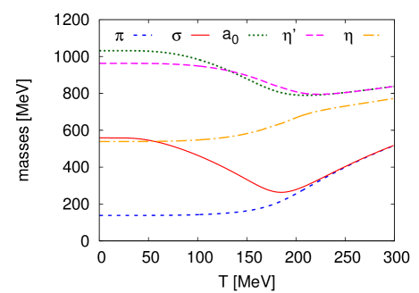
(a)   with $U(1)_{A}$-symmetry breaking

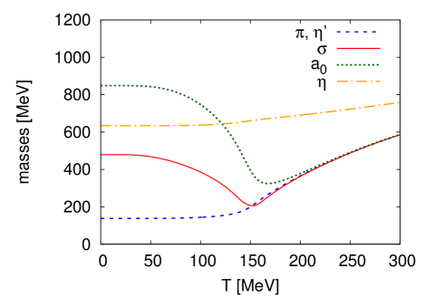
(b)   without $U(1)_{A}$-symmetry breaking

Figure 1: Meson masses obtained with the FRG as a function of the temperature for vanishing chemical potentials.

V Results and Discussion

In this section we discuss and compare the phase structure of the $(2+1)$-flavor quark-meson model in different approximations. We focus on the chiral phase transition at finite temperature and flavor symmetric chemical potential and consider homogeneous chiral condensates. Any inhomogeneities which might be of relevance at low temperatures and intermediate quark densities, see e.g. Nickel:2009wj , are thus excluded. We thoroughly investigate the interplay of quantum and thermal fluctuations with the anomalous $U(1)_{A}$-symmetry breaking via Eq. (5). Consequences for the location of the critical endpoint in the phase diagram as well as the order of the chiral transition in the limit of vanishing light quark masses are discussed. We compare results obtained with a full functional renormalization group (FRG) analysis, a mean-field approximation (MFA) and with a modified FRG approximation where meson loop contributions are dropped. The latter approximation is equivalent to the so-called extended mean-field approximation where the renormalized fermionic vacuum sea term is included in the grand potential (eMFA), see Andersen:2011pr ; Skokov:2010sf and Sec. III. Further technical details concerning the numerical solution of the flow equation can be found in the appendices A and B. All parameters of the model are fixed in such a way that experimental observables like the pion decay constant and meson masses are reproduced in the vacuum, see appendix A.2 for details.

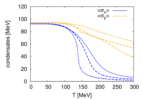
(a)   with $U(1)_{A}$-symmetry breaking

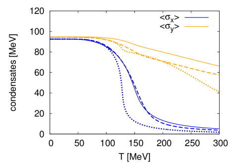
(b)   without $U(1)_{A}$-symmetry breaking

Figure 2: Non-strange $\left\langle\sigma_{x}\right\rangle$ and strange $\left\langle\sigma_{y}\right\rangle$ condensates for vanishing chemical potentials in different approximations (solid lines: FRG, dotted lines: standard MFA and dashed lines: extended MFA) .

V.1 Chiral Crossover and Axial Anomaly

First we investigate the $U(1)_{A}$-symmetry breaking and the influence of thermal fluctuations on the chiral crossover at vanishing chemical potential $\mu=0$. In Fig. 1 we show FRG results for the (pseudo)scalar non-strange and $\eta$, $\eta^{\prime}$-meson masses as a function of the temperature $T$. In the left panel the $U(1)_{A}$-symmetry is broken via Eq. (5). Without this $U(1)_{A}$-symmetry breaking (right panel) the $\eta^{\prime}$-meson mass degenerates always with the pion mass and the two sets of light chiral partners $(\sigma,\vec{\pi})$ and $(\vec{a}_{0},\eta^{\prime})$ collapse in the chirally symmetric phase.

In agreement with experiment Vertesi:2009wf ; *Csorgo2010, we find for a broken $U(1)_{A}$-symmetry that the mass of the $\eta^{\prime}$-meson drops around the chiral crossover. The drop of the mass at the chiral transition is a consequence of the Kobayashi-Maskawa-’t Hooft term, Eq. (5), for three flavors. It is cubic in the fields $\sigma_{x}$, $\sigma_{y}$ and hence the anomalous contribution to $m^{2}_{\eta^{\prime}}$ depends linearly on the condensates $\left\langle\sigma_{x}\right\rangle$ and $\left\langle\sigma_{y}\right\rangle$ which both melt at the crossover. This is demonstrated in Fig. 2, where both condensates, including the anomaly (left panel) and without the anomaly (right panel), are shown as a function of the temperature for vanishing chemical potential. In the standard MFA the condensates decrease faster than in approximations including fluctuations. The value of the pseudocritical temperature, defined by the inflection point of the non-strange condensates, varies by 10% without the anomaly and by 20% including the anomaly. The largest shift of the critical temperature in comparison to the standard MFA is seen with the full FRG: fluctuations smoothen and push the non-strange transition to higher temperatures. This trend is similar to previous two-flavor investigations, see e.g. Nakano:2009ps .

Furthermore, the slope of the crossover is modified by mesonic fluctuations and depends on the axial $U(1)_{A}$-anomaly. Interestingly, without the anomaly (right panel) the extended MFA and FRG results for the non-strange condensate almost coincide for all temperatures. With determinant, on the other hand, the crossover is washed out even further by the mesonic fluctuations.

The strange sector is only mildly affected by the Kobayashi-Maskawa-’t Hooft determinant and the strange condensate melts only moderately, see Fig. 2. Independent of the used approximation the rather slow melting of the strange condensate might be related, at least partially, to the fit procedure of the model parameters. It has been observed previously that for low values of the sigma meson mass, all condensates vanish in the $SU(3)$ chiral limit. As a consequence, spontaneous chiral symmetry breaking is lost Schaefer:2008hk and the value of the strange condensate is mainly governed by the large and temperature-independent explicit symmetry breaking parameter $c_{y}$. Correspondingly, we expect a considerably smaller temperature dependence of the strange sector compared to the light one.

Finally, the strange condensate melts even slower when mesonic fluctuations are taken into account. This might lead to the conclusion that the temperature-dependence of a $U(1)_{A}$-symmetry breaking term is mostly driven by the non-strange sector. Work in this direction is in progress mmanomalie .

V.2 Finite density and the critical endpoint

In the following we explore how the location of the critical endpoint (CEP) in the phase diagram is affected by fluctuations with and without anomalous $U(1)_{A}$-symmetry breaking. The location of the CEP also depends considerably on the chosen value of the $\sigma$-meson mass Schaefer:2008hk . To eliminate this $m_{\sigma}$-dependence, we fix the value to $m_{\sigma}=480$ MeV, unless stated otherwise.

$c$ [MeV]	MFA	eMFA	FRG
$4807.84$	$(98,155)$	$(35,293)$	$(17,295)$
$0$	$(93,173)$	$(31,298)$	$(43,280)$

Table 1: Critical endpoint coordinates $(T_{c},\mu_{c})$ in units of MeV for different approximations with and without anomaly.

Results for the location of the CEP obtained with our various approximations to the grand potential are summarized in Tab. 1. In agreement with previous investigations Schaefer:2008hk , we find that in a standard mean-field approximation the CEP is pushed towards smaller chemical potentials and higher temperatures if the $U(1)_{A}$-symmetry violation is taken into account. Adding the fermionic vacuum contribution to the potential, this behavior with respect to the anomaly does not change qualitatively, although the CEP is pushed towards considerably larger densities and smaller temperatures. In contrast, by additionally taking mesonic fluctuations into account, the dependency on the anomalous $U(1)_{A}$-symmetry breaking is reversed. With a constant Kobayashi-Maskawa-’t Hooft determinant, the endpoint is pushed towards larger chemical potentials and smaller temperatures. It is remarkable that the endpoint without anomaly, but with mesonic fluctuations is located at larger temperatures and smaller chemical potentials than for the eMFA.

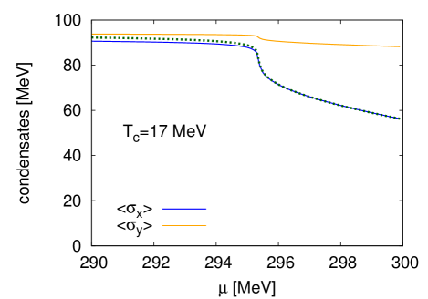
(a)   with $U(1)_{A}$-symmetry breaking

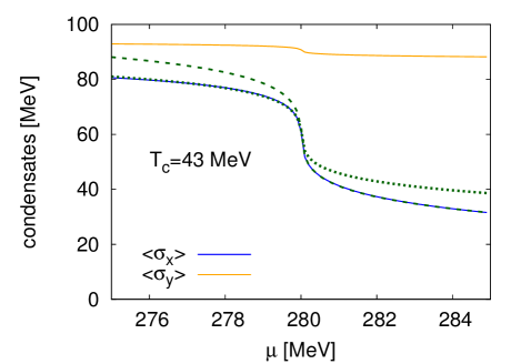
(b)   without $U(1)_{A}$-symmetry breaking

Figure 3: The condensates in the vicinity of the critical point as a function of the chemical potential ($m_{\sigma}=480$ MeV). Dotted and dashed lines are fit functions. See text for details.

Although it is well-established that $U(1)_{A}$-symmetry breaking terms are suppressed at asymptotically large temperatures and chemical potentials Gross:1980br ; *Schafer:1996wv; *Schafer:2002ty, it is not fully settled whether this also holds at intermediate temperatures and chemical potentials Costa:2004db . Recent lattice investigations indicate, however, that the $U(1)_{A}$-symmetry might already be effectively restored at temperatures slightly above the chiral crossover Bazavov:2012qja ; Cossu:2012gm ; *Cossu:2013uua. Then our findings also have consequences on the location of the CEP in two-flavor investigations. In such studies one usually assumes maximal $U(1)_{A}$-symmetry breaking by considering only the $(\sigma,\vec{\pi})$-mesons. The $(\eta,\vec{a})$-mesons decouple due to their assumed large masses, which are induced by the large Kobayashi-Maskawa-’t Hooft determinant Jungnickel1996b . If, however, the $U(1)_{A}$-symmetry is restored with chiral symmetry, we expect that the critical endpoint is shifted towards larger temperatures and lower chemical potentials also in a two flavor scenario. Thus, a direct confirmation of this scenario requires investigations which also include the $(\eta,\vec{a})$-mesons mmanomalie . This also concerns phase structure studies in terms of QCD degrees of freedom, e.g. Braun:2009gm ; *Pawlowski:2010ht; *Fischer:2011mz; *Fischer:2012vc; *Fischer:2013eca.

In Fig. 3 both condensates with (left) and without anomaly (right) are plotted in the vicinity of the critical point as a function of the chemical potential. Similar to the crossover at $\mu=0$, the strange condensate melts considerably less than the light condensate around the CEP in all approximations. Interestingly, the two condensates seem to be related to each other at criticality. We found a scaling between both condensates that is demonstrated in Fig. 3 with dashed and dotted lines which are obtained by the ansatz $\left\langle\sigma_{x}\right\rangle=\alpha_{1}+\alpha_{2}\langle\sigma_{y}\rangle$ with the two constant fit parameters $\alpha_{i}$. In particular, with $U(1)_{A}$-symmetry breaking (left panel) we see an almost perfect scaling in both regions while without anomaly (right panel) the scaling depends on which phase we use to fit the parameters.

The dependency of the CEP location in the phase diagram on the $U(1)_{A}$-symmetry and also on the sigma mass $m_{\sigma}$ is demonstrated in Fig. 4, where the FRG result for the quark number susceptibility in the vicinity of the critical point, normalized with the quark chemical potential, is shown as a function of the chemical potential. In this figure two different CEP scenarios are compared with each other. First, fixing the sigma mass to $m_{\sigma}=480$ MeV (solid, red and dashed, blue lines) the point is pushed towards the temperature axis for a $U(1)_{A}$-symmetric theory. Second, reducing the sigma mass to $m_{\sigma}=400$ MeV but fixing the $U(1)_{A}$-symmetry breaking the CEP is also pushed towards the temperature axis (solid, red and dotted, green lines).

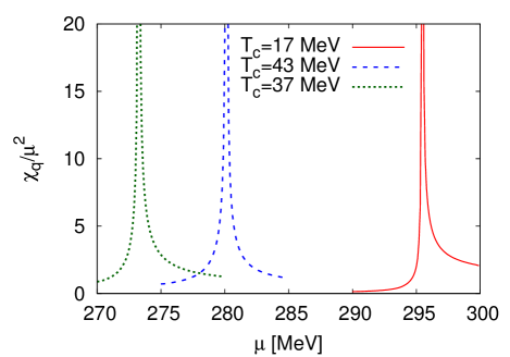
Figure 4: Quark number susceptibility in the vicinity of the critical point without $U(1)_{A}$-symmetry for $m_{\sigma}=480$ MeV (solid, red) and for $m_{\sigma}=400$ MeV (dotted, green). For comparison, the $U(1)_{A}$-symmetric susceptibility for $m_{\sigma}=480$ MeV (dashed, blue) is also shown.

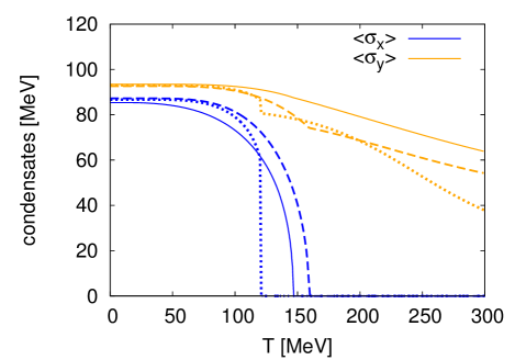
(a)   with $U(1)_{A}$-symmetry breaking

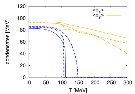
(b)   without $U(1)_{A}$-symmetry breaking

Figure 5: Non-strange $\left\langle\sigma_{x}\right\rangle$ and strange $\left\langle\sigma_{y}\right\rangle$ condensates in the non-strange chiral limit for $\mu=0$ obtained in different approximations similar to Fig. 2 (solid lines: FRG, dotted lines: standard MFA and dashed lines: extended MFA).

V.3 Chiral Limits

Finally, we investigate the quark mass sensitivity of the chiral transition including the anomaly and examine various chiral limits.

Based on RG arguments for a purely bosonic theory, the chiral transition is of first order in the $SU(3)$-symmetric chiral limit, whereas the order of the transition in the two-flavor chiral limit depends on the implementation of the $U(1)_{A}$-symmetry breaking Pisarski1984a . For a $U(1)_{A}$-symmetric two flavor system with $U(2)_{L}\times U(2)_{R}$ symmetry a first-order transition is expected in the chiral limit, see e.g. Fukushima:2010ji ; Grahl:2013pba . With an axial $U(1)_{A}$-symmetry breaking the order can change to second order if the coupling strength of the Kobayashi-Maskawa-’t Hooft determinant is only moderately temperature dependent. Therefore, a temperature independent, i.e. constant, $U(1)_{A}$-symmetry breaking can smoothen the transition from first to second order in the two-flavor chiral limit, whereas the opposite happens for three flavors and the first-order transition becomes even stronger in the corresponding chiral limit.

Relative to the anomalous $U(1)_{A}$-symmetry implementation, several scenarios in the light and strange quark mass $(m_{l},m_{s})$-plane can now arise. Around the $SU(3)$-symmetric chiral limit with $(m_{l},m_{s})=(0,0)$ there might be a finite region of first-order transitions with a second-order boundary line, which terminates at a finite value of a tricritical strange mass, $m^{*}_{s}$, from which a second-order transition line is extended to the two flavor chiral limit. The precise location and even the existence of such a tricritical strange quark mass $m^{*}_{s}$ is not yet fully settled. However, there could also be a first-order region connecting the $SU(3)$ and the two-flavor chiral limits along the $(m_{l}=0)$-line, see e.g. Schaefer:2008hk ; Aoki:2012yj . Then, there should not be a critical value of the strange quark mass $m_{s}^{*}$, but a critical light quark mass $m_{l}^{*}$ in the two flavor case.

Independent of the $U(1)_{A}$-symmetry breaking, a first-order transition is seen in quark-meson models in standard mean-field approximations in the two-flavor as well as in the $SU(3)$-symmetric chiral limit, see e.g. Schaefer:2004en ; Schaefer:2008hk . For an explicit symmetry breaking strength $c_{y}=c_{y,\text{phys}}$ that leads to a strange constituent quark mass of $m_{s}=430$ MeV we also find a first-order transition in the non-strange chiral limit, see Fig. 5, where both order parameters in different approximations are plotted in the non-strange chiral limit. However, as already argued in Skokov:2010sf , the first-order transition might be misleading and an artifact of the used mean-field approximation. Going beyond mean-field approximations by taking the vacuum fluctuations of the quarks into account (eMFA), this behavior is changed and a second-order transition is observed, which is independent of the axial anomaly (see dashed lines in the figure). When mesonic fluctuations are considered in addition via a full FRG treatment, the order of the transition depends on the anomaly. Including the Kobayashi-Maskawa-’t Hooft determinant, a second-order transition is found while for a $U(1)_{A}$-symmetric theory the transition becomes first-order (solid lines).

This agrees with the picture that the chiral transition is mostly driven by two flavor dynamics, i.e., the non-strange chiral limit behaves qualitatively more like the $SU(2)$-symmetric than the $SU(3)$-symmetric chiral limit. As a consequence, the $U(1)_{A}$-symmetry violating and temperature independent determinant acts like a mass term, which leads to a second-order transition as in Pisarski1984a .

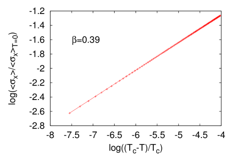
Figure 6: Scaling of the non-strange condensate close to the critical point. The slope corresponds to the $O(4)$ critical exponent $\beta=0.39$.

Without the Kobayashi-Maskawa-’t Hooft term we have also investigated the shape of the first-order region by varying the explicit symmetry breaking parameter $c_{y}$ around its physical value $c_{y,\text{phys}}$. In this way we have determined with the FRG the corresponding $c^{*}_{x}$ that leads to a second-order chiral transition. Since the value of the critical $c^{*}_{x}$ also depends on the chosen coarse graining scale in the infrared Litim:1994jd ; *Litim:1996nw; *Berges:1996ib, we can only determine a qualitative picture of the first-order region. For example, in Fig. 5 an infrared cutoff of the order of $100$ MeV has been employed. Schematically, we find that the critical $c^{*}_{x}$ grows with $c_{y}$ around its physical value $c_{y,\text{phys}}$. A similar behavior has also been found in a purely mesonic study Lenaghan:2000kr and is consistent with the scenario that the first-order region is extended along the $(m_{l}=0)$-line without anomalous $U(1)_{A}$-symmetry breaking.

For the second-order transition, we find critical exponents which lie in the $O(4)$-universality class. For example, we find $\beta=0.39$, as demonstrated in the Fig. 6, where the scaling of the order parameter over several orders of magnitudes is displayed. Since the anomalous dimension vanishes in leading-order derivative expansion of the average effective action, $\eta\equiv 0$, the remaining critical exponents are given by (hyper)scaling relations. The $O(4)$ critical exponents are a consequence of the finite Kobayashi-Maskawa-’t Hooft coupling at the critical temperature. If, however, the $U(1)_{A}$-symmetry were effectively restored at the chiral transition, we would expect critical exponents in the $U(2)_{L}\times U(2)_{R}/U(2)_{V}$ universality class in case of a second-order transition Basile:2005hw ; *Vicari:2007ma; Aoki:2012yj ; Grahl:2013pba .

VI Summary and conclusions

We have investigated the consequences of anomalous $U(1)_{A}$-symmetry breaking in the presence of quantum and thermal fluctuations in a three flavor effective description for QCD with a focus on the phase structure. With an effective quark-meson model a drop of the anomalous mass of the $\eta^{\prime}$-meson at the chiral crossover temperature is found which agrees well with recent experiments. In analogy to a corresponding two flavor description fluctuations weaken the chiral crossover and the chiral condensates decrease less rapidly. In particular, the strange condensate melts considerably slower when fluctuations are taken into account. This leads to the conclusion that the chiral dynamic around the crossover is predominantly governed by the light quark sector.

At finite quark chemical potential, mesonic fluctuations lead to a considerable effect in the presence of an anomalous $U(1)_{A}$-symmetry breaking realized by a Kobayashi-Maskawa-’t Hooft determinant in the Lagrangian. Without anomalous $U(1)_{A}$-symmetry breaking the endpoint is pushed to significantly larger temperatures and smaller chemical potentials. This strong dependency of the CEP location on $U(1)_{A}$-symmetry breaking is opposite to what is found in corresponding mean-field investigations. Hence, for future investigations on the existence/location of a possible critical endpoint in the QCD phase diagram it is crucial to consider all quantum and thermal fluctuations with a proper $U(1)_{A}$-symmetry breaking and its possible effective restoration.

Finally, we have investigated the order of the chiral transition in the limit of vanishing light, but physical strange quark masses. In standard mean-field approximations we find, independent of the anomalous $U(1)_{A}$-symmetry breaking, a first-order transition and a second-order transition if the vacuum term is included. However, with mesonic fluctuations the transition is of first-order without the axial $U(1)_{A}$-anomaly and of second-order with the anomaly, lying in the $O(4)$-universality class. This demonstrates once more the importance of the interrelation of mesonic fluctuations with the chiral $U(1)_{A}$-anomaly. Furthermore, in agreement with other model studies without quarks, e.g. Lenaghan:2000kr , we find for growing light quark masses that the first-order region in the ($m_{l}$, $m_{s}$)-plane is extended to larger strange quark masses if the anomaly is neglected.

Acknowledgments

We thank T.K. Herbst, J.M. Pawlowski, R. Stiele and M. Wagner for interesting and enlightening discussions. M.M. acknowledges support by the FWF through DK-W1203-N16, the Helmholtz Alliance HA216/EMMI, and the BMBF grant OSPL2VHCTG. B.-J.S. acknowledges support by the FWF grant P24780-N27 and by CompStar, a research networking programme of the European Science Foundation. This work is supported by the Helmholtz International Center for FAIR within the LOEWE program of the State of Hessen.

Appendix A Numerical implementations

In this appendix some technical details of the used two-dimensional grid and Taylor expansion technique for the numerical solution of the flow equation are given. At the end of this appendix the procedure for fixing the initial parameters for the flow equations is summarized.

A.1 Two-dimensional grid and Taylor technique

For the construction of the two-dimensional grid we define the positive variables

$$x=\sigma_{x}^{2},\quad y=2\sigma_{y}^{2}-\sigma_{x}^{2}\ .$$ (27)

Clamped cubic splines are used to evaluate the required first- and second-order derivatives of the effective potential as a function of $x$ and $y$, see also Strodthoff:2011tz . Derivatives of the effective potential with respect to the chiral invariants are obtained by applying the chain rule.

For comparison, a Taylor expansion of the effective potential in the variables $\rho_{1}$ and $\tilde{\rho}_{2}$ is performed to order $\mathcal{O}\left(\rho_{i}^{3}\right)$ around the $k$-dependent minimum. The scale dependence of the minimum is used to replace the flow of the Taylor coefficients $a_{10}$ and $a_{01}$ via the conditions

$$\partial_{\sigma_{x}}U_{k}\big{|}_{\text{min}}=\partial_{\sigma_{y}}U_{k}\big{|}_{\text{min}}=0\ .$$ (28)

The convergence properties of such expansion schemes have been studied in, e.g., Tetradis:1993ts ; Papp2000 .

In both numerical approaches, the right hand side of the flow equation (25) requires the knowledge of the eigenvalues of the Hessian of the effective potential with respect to all mesonic fields $\Sigma$. The Hessian is given in terms of derivatives of the effective potential with respect to the chiral invariants $\rho_{1}$ and $\tilde{\rho}_{2}$. The resulting expressions are summarized in App. B. Then, the flow equation becomes a coupled set of non-linear ordinary differential equations for either the values of the effective potential at the interpolated grid points or for the Taylor expansion coefficients (beta-functions), which can be solved with standard numerical methods. A numerical comparison of both techniques is given in Fig. 7, where the meson masses are plotted as a function of the temperature for $\mu=0$. Both methods agree very well, at least for small chemical potentials, see also Nakano:2009ps .

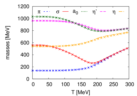
Figure 7: Meson masses obtained with the grid method (solid lines) and with the Taylor expansion technique (crosses).

A.2 Initial condition

In order to solve the flow equation the initial action has to be specified at a given UV scale. Explicitly, as initial potential at $\Lambda=1$ GeV we use the expression

$$U_{\Lambda} = \tilde{U}_{\Lambda}(\rho_{1},\tilde{\rho}_{2})-c\xi-c_{x}\sigma_{x}-c_{y}\sigma_{y}$$ (29)

with

$$\tilde{U}_{\Lambda}(\rho_{1},\tilde{\rho}_{2}) = a_{10,\Lambda}\rho_{1}+\frac{a_{20,\Lambda}}{2}\rho_{1}^{2}+a_{01,\Lambda}\tilde{\rho}_{2}\ .$$

and fix the Yukawa coupling $h$ such that physical values for the pion and kaon decay constants $f_{\pi}$ and $f_{K}$, the pion and kaon masses $m_{\pi}$ and $m_{K}$, the combined $\eta$ and $\eta^{\prime}$ masses $m_{\eta}^{2}+m_{\eta^{\prime}}^{2}$, the sigma mass $m_{\sigma}$ and the light constituent quark mass $m_{l}$ are obtained in the infrared. In contrast to a mean-field treatment Schaefer:2008hk it is not possible to choose arbitrary values for the mesonic potential in the infrared. Especially, the sigma meson mass is restricted to values between approximately $400$ and $600$ MeV for physical pion masses $m_{\pi}\approx 140$ MeV. We use $h=6.5$, $c_{x}=(120.73$ MeV$)^{3}$ and $c_{y}=(336.41$ MeV$)^{3}$ together with $a_{10,\Lambda}$, $a_{01,\Lambda}$ and $a_{20,\Lambda}$ as given in Tab. 2.

$m_{\sigma}$ [MeV]	$c$ [MeV]	$a_{10,\Lambda}$ [MeV2]	$a_{01,\Lambda}$	$a_{20,\Lambda}$
$480$	$0$	$(178.88)^{2}$	$140$	$25$
$400$	$4807.84$	$(972.63)^{2}$	$50$	$2.5$
$480$	$4807.84$	$(867.76)^{2}$	$50$	$12$
$560$	$4807.84$	$(542.22)^{2}$	$50$	$36$

Table 2: Parameters for the initial potential.

Fixing the parameters in the vacuum, the finite temperature results are then predictions.

Appendix B Meson Masses

In this section the explicit expressions for the mesonic screening masses are collected. They are derived from the potential

$$U_{k}(\Sigma) = \tilde{U}_{k}(\rho_{1},\tilde{\rho}_{2})-c\xi-c_{x}\sigma_{x}-c_{y}\sigma_{y}\ ,$$ (30)

with isospin symmetry, i.e., for $\langle\sigma_{3}\rangle=0$.

The squared masses are defined by the eigenvalues of the Hessian matrix of the effective potential $\nabla_{\Sigma}^{2}U_{k}=\nabla_{\Sigma}^{2}\tilde{U}_{k}-c\nabla_{\Sigma}^{2}\xi$ with

$$\nabla_{\Sigma}^{2}\tilde{U}_{k} = \left(\partial_{\rho_{1}}\tilde{U}_{k}\right)\nabla_{\Sigma}^{2}\rho_{1}+\left(\partial_{\tilde{\rho}_{2}}\tilde{U}_{k}\right)\nabla_{\Sigma}^{2}\tilde{\rho}_{2}$$

$$+\left(\partial_{\rho_{1}}^{2}\tilde{U}_{k}\right)(\nabla_{\Sigma}\rho_{1})^{T}\nabla_{\Sigma}\rho_{1}-c\nabla_{\Sigma}^{2}\xi$$

$$+\left(\partial_{\tilde{\rho}_{2}}^{2}\tilde{U}_{k}\right)(\nabla_{\Sigma}\tilde{\rho}_{2})^{T}\nabla_{\Sigma}\tilde{\rho}_{2}$$

$$+\left(\partial_{\rho_{1}}\partial_{\tilde{\rho}_{2}}\tilde{U}_{k}\right)\left[(\nabla_{\Sigma}\rho_{1})^{T}\nabla_{\Sigma}\tilde{\rho}_{2}+(\nabla_{\Sigma}\tilde{\rho}_{2})^{T}\nabla_{\Sigma}\rho_{1}\right]\ .$$

Hence, the mesonic masses can be calculated from derivatives of $\tilde{U}_{k}$ with respect to the invariants $\rho_{1}$ and $\tilde{\rho}_{2}$ together with the gradient and Hessian of the invariants with respect to $\Sigma=(\sigma_{x},\sigma_{1},\dots\sigma_{7},\sigma_{y},\pi_{0},\dots,\pi_{8})$. The latter are given by

$$(\nabla_{\Sigma}\rho_{1})_{1}=\sigma_{x}\ , \qquad(\nabla_{\Sigma}\rho_{1})_{8}=\sigma_{y}\ ,$$ (32)

$$(\nabla_{\Sigma}^{2}\rho_{1})_{i,i}=1\ , \quad i=1,\dots,18\ ,$$ (33)

$$(\nabla_{\Sigma}\tilde{\rho}_{2})_{1} =\sigma_{x}\frac{(\sigma_{x}^{2}-2\sigma_{y}^{2})}{6}\ ,$$ (34)

$$(\nabla_{\Sigma}\tilde{\rho}_{2})_{8} =-\sigma_{y}\frac{(\sigma_{x}^{2}-2\sigma_{y}^{2})}{3}\ ,$$

$$(\nabla_{\Sigma}^{2}\tilde{\rho}_{2})_{1,1} =\frac{3\ \sigma_{x}^{2}-2\ \sigma_{y}^{2}}{6}\ ,$$

$$(\nabla_{\Sigma}^{2}\tilde{\rho}_{2})_{9,9} =\frac{-\sigma_{x}^{2}+6\ \sigma_{y}^{2}}{3}\ ,$$ (35a)

$$(\nabla_{\Sigma}^{2}\tilde{\rho}_{2})_{1,9} =-\frac{2\ \sigma_{x}\sigma_{y}}{3}\ ,$$

$$(\nabla_{\Sigma}^{2}\tilde{\rho}_{2})_{i,i} =\frac{7\ \sigma_{x}^{2}-2\ \sigma_{y}^{2}}{6}\ ,\quad i=2,3,4\ ,$$ (35b)

$$(\nabla_{\Sigma}^{2}\tilde{\rho}_{2})_{i,i} =\frac{\sigma_{x}^{2}+\sqrt{18}\ \sigma_{x}\sigma_{y}+4\ \sigma_{y}^{2}}{6}\ ,\quad i=5,\dots,8\ ,$$

$$(\nabla_{\Sigma}^{2}\tilde{\rho}_{2})_{10,10} =0\ ,$$

$$(\nabla_{\Sigma}^{2}\tilde{\rho}_{2})_{18,18} =\frac{-\sigma_{x}^{2}+2\ \sigma_{y}^{2}}{6}\ ,$$ (35c)

$$(\nabla_{\Sigma}^{2}\tilde{\rho}_{2})_{10,18} =\frac{\sigma_{x}^{2}-2\ \sigma_{y}^{2}}{3\sqrt{2}}\ ,$$

$$(\nabla_{\Sigma}^{2}\tilde{\rho}_{2})_{i,i} =\frac{\sigma_{x}^{2}-2\ \sigma_{y}^{2}}{6}\ ,\quad i=11,12,13\ ,$$ (35d)

$$(\nabla_{\Sigma}^{2}\tilde{\rho}_{2})_{i,i} =\frac{\sigma_{x}^{2}-\sqrt{18}\ \sigma_{x}\sigma_{y}+4\ \sigma_{y}^{2}}{6}\ ,\quad i=14,\dots,17\ ,$$

$$(\nabla_{\Sigma}^{2}\xi)_{1,1} =\frac{\sigma_{y}}{\sqrt{2}}\ ,$$

$$(\nabla_{\Sigma}^{2}\xi)_{9,9} =0\ ,$$ (36a)

$$(\nabla_{\Sigma}^{2}\xi)_{1,9} =\frac{\sigma_{x}}{\sqrt{2}}\ ,$$

$$(\nabla_{\Sigma}^{2}\xi)_{i,i} =-\frac{\sigma_{y}}{\sqrt{2}}\ ,\quad i=2,3,4\ ,$$ (36b)

$$(\nabla_{\Sigma}^{2}\xi)_{i,i} =-\frac{\sigma_{x}}{2}\ ,\quad i=5,\dots,8\ ,$$

$$(\nabla_{\Sigma}^{2}\xi)_{10,10} =\frac{-2\ \sigma_{x}-\sqrt{2}\ \sigma_{y}}{3}\ ,$$

$$(\nabla_{\Sigma}^{2}\xi)_{18,18} =\frac{5\ \sigma_{x}-\sqrt{2}\ \sigma_{y}}{6}\ ,$$ (36c)

$$(\nabla_{\Sigma}^{2}\xi)_{10,18} =\frac{\sqrt{2}\ \sigma_{x}-2\ \sigma_{y}}{6}\ ,$$

$$(\nabla_{\Sigma}^{2}\xi)_{i,i} =\frac{\sigma_{y}}{\sqrt{2}}\ ,\quad i=11,12,13\ ,$$ (36d)

$$(\nabla_{\Sigma}^{2}\xi)_{i,i} =\frac{\sigma_{x}}{2}\ ,\quad i=14,\dots,17$$

where the subscripts $i$ denote the components of the vectors and matrices, respectively. Hence, the Hessian splits into a (pseudo)scalar $(9\times 9)$-mass matrix ($M^{2}_{ps}$) $M^{2}_{s}$

$$\nabla_{\Sigma}^{2}U_{k} = \begin{pmatrix}M^{2}_{s}&0\\ 0&M^{2}_{ps}\end{pmatrix}\ ,$$ (37)

where the only nonvanishing off-diagonal entries in each submatrix are the $1$, $9$ components.

Note that in a mean-field treatment there is an additional quark contribution to the effective potential, which also modifies the Hessian, see Ref. Schaefer:2008hk for explicit expressions. For a renormalization group treatment, on the other hand, these contributions are naturally included in the IR solution of the potential $U_{k\rightarrow 0}$.

References

- (1) S. L. Adler and W. A. Bardeen, Phys.Rev. 182, 1517 (1969);
- (2) J. Bell and R. Jackiw, Nuovo Cim. A60, 47 (1969);
- (3) K. Fujikawa, Phys. Rev. Lett. 42, 1195 (1979).
- (4) S. Weinberg, Phys.Rev. D11, 3583 (1975).
- (5) G. Christos, Phys.Rept. 116, 251 (1984).
- (6) G. ’t Hooft, Phys. Rept. 142, 357 (1986).
- (7) G. ’t Hooft, Phys.Rev.Lett. 37, 8 (1976);
- (8) G. ’t Hooft, Phys.Rev. D14, 3432 (1976).
- (9) E. Witten, Nucl. Phys. B156, 269 (1979);
- (10) G. Veneziano, Nucl. Phys. B159, 213 (1979).
- (11) M. G. Alford, A. Schmitt, K. Rajagopal, T. Schäfer, Rev. Mod. Phys. 80, 1455 (2008).
- (12) D. Nickel, Phys. Rev. D80, 074025 (2009).
- (13) B. Friman, C. Hohne, J. Knoll, S. Leupold, J. Randrup, et al., Lect.Notes Phys. 814, 1 (2011).
- (14) D. J. Gross, R. D. Pisarski, and L. G. Yaffe, Rev.Mod.Phys. 53, 43 (1981);
- (15) T. Schäfer and E. V. Shuryak, Rev.Mod.Phys. 70, 323 (1998).
- (16) T. Schäfer, Phys.Rev. D65, 094033 (2002).
- (17) T. D. Cohen, Phys.Rev. D54, 1867 (1996);
- (18) S. H. Lee and T. Hatsuda, Phys.Rev. D87, 1871 (1996);
- (19) M. C. Birse, T. D. Cohen and J. A. McGovern, Phys.Lett. B388, 137 (1996);
- (20) G. V. Dunne and A. Kovner, Phys.Rev. D82, 065014 (2010).
- (21) R. Vertesi, T. Csorgo, and J. Sziklai, Phys.Rev. C83, 054903 (2011);
- (22) T. Csorgo, R. Vertesi, and J. Sziklai, Phys. Rev. Lett. 105, 182301 (2010).
- (23) J. I. Kapusta, D. Kharzeev, and L. D. McLerran, Phys.Rev. D53, 5028 (1996).
- (24) A. Bazavov et al. (HotQCD Collaboration), Phys.Rev. D86, 094503 (2012).
- (25) G. Cossu, S. Aoki, S. Hashimoto, T. Kaneko, H. Matsufuru, et al., PoS LATTICE2011, 188 (2011);
- (26) G. Cossu, S. Aoki, H. Fukaya, S. Hashimoto, T. Kaneko, et al. (2013).
- (27) S. Muroya, A. Nakamura, C. Nonaka, and T. Takaishi, Prog.Theor.Phys. 110, 615 (2003);
- (28) O. Philipsen, Eur.Phys.J.ST 152, 29 (2007).
- (29) J. Berges, N. Tetradis, and C. Wetterich, Phys. Rept. 363, 223 (2002);
- (30) K. Aoki, Int.J.Mod.Phys. B14, 1249 (2000);
- (31) J. M. Pawlowski, Annals Phys. 322, 2831 (2007);
- (32) B.-J. Schaefer and J. Wambach, Phys. Part. Nucl. 39, 1025 (2008);
- (33) H. Gies, Lect. Notes Phys. 852 pp. 287–348 (2012);
- (34) J. Braun, J.Phys. G39, 033001 (2012).
- (35) J. M. Pawlowski, Phys. Rev. D58, 045011 (1998);
- (36) L. von Smekal, A. Mecke, and R. Alkofer, Big Sky 1997, Intersections between particle and nuclear physics p. 746 (1997);
- (37) R. Alkofer, C. S. Fischer, and R. Williams, Eur.Phys.J. A38, 53 (2008).
- (38) S. Benic, D. Horvatic, D. Kekez, and D. Klabucar, Phys.Rev. D84, 016006 (2011).
- (39) J. Braun, L. M. Haas, F. Marhauser, and J. M. Pawlowski, Phys.Rev.Lett. 106, 022002 (2011);
- (40) J. M. Pawlowski, AIP Conf.Proc. 1343, 75 (2011);
- (41) C. S. Fischer, L. Fister, J. Luecker, and J. M. Pawlowski, arXiv:1306.6022 [hep-ph];
- (42) C. S. Fischer, J. Luecker, and J. A. Mueller, Phys.Lett. B702, 438 (2011)
- (43) C. S. Fischer and J. Luecker, Phys.Lett. B718, 1036 (2013).
- (44) D. U. Jungnickel and C. Wetterich, Phys. Rev. D53, 5142 (1996).
- (45) J. Berges, D. U. Jungnickel, and C. Wetterich, Phys. Rev. D59, 034010 (1999);
- (46) B.-J. Schaefer and H.-J. Pirner, Nucl. Phys. A660, 439 (1999);
- (47) J. Braun, K. Schwenzer, and H.-J. Pirner, Phys. Rev. D70, 085016 (2004).
- (48) B.-J. Schaefer and J. Wambach, Nucl. Phys. A757, 479 (2005);
- (49) B.-J. Schaefer and J. Wambach, Phys.Rev. D75, 085015 (2007).
- (50) H. Gies and C. Wetterich, Phys.Rev. D69, 025001 (2004);
- (51) J. Braun, Eur.Phys.J. C64, 459 (2009).
- (52) R. D. Pisarski and F. Wilczek, Phys. Rev. D29, 338 (1984).
- (53) J. Schaffner-Bielich, Phys.Rev.Lett. 84, 3261 (2000).
- (54) J. T. Lenaghan, Phys. Rev. D63, 037901 (2001).
- (55) T. Hatsuda, M. Tachibana, N. Yamamoto and G. Baym, Phys. Rev. Lett. 97, 122001 (2006);
- (56) N. Yamamoto, M. Tachibana, T. Hatsuda and G. Baym, Phys. Rev. D76, 074001 (2007).
- (57) S. Chandrasekharan and A. C. Mehta, Phys.Rev.Lett. 99, 142004 (2007).
- (58) J.-W. Chen, K. Fukushima, H. Kohyama, K. Ohnishi, and U. Raha, Phys. Rev. D80, 054012 (2009).
- (59) B.-J. Schaefer and M. Wagner, Phys. Rev. D79, 014018 (2009).
- (60) M. Kobayashi and T. Maskawa, Prog.Theor.Phys. 44, 1422 (1970).
- (61) J. S. Schwinger, Annals Phys. 2, 407 (1957);
- (62) M. Gell-Mann and M. Levy, Nuovo Cim. 16, 705 (1960).
- (63) H. Meyer-Ortmanns, H. J. Pirner, and A. Patkos, Phys. Lett. B295, 255 (1992);
- (64) H. Meyer-Ortmanns and B.-J. Schaefer, Phys. Rev. D53, 6586 (1996).
- (65) D.-U. Jungnickel and C. Wetterich, Eur. Phys. Jour. C2, 557 (1998);
- (66) J. T. Lenaghan, D. H. Rischke, and J. Schaffner-Bielich, Phys. Rev. D62, 085008 (2000);
- (67) O. Scavenius, A. Mocsy, I. N. Mishustin, and D. H. Rischke, Phys. Rev. C64, 045202 (2001).
- (68) A. Patkos, Mod.Phys.Lett. A27, 1250212 (2012).
- (69) D. Klabucar, D. Kekez, and M. D. Scadron, J.Phys. G27, 1775 (2001);
- (70) P. Kovacs and Z. Szep, Phys.Rev. D77, 065016 (2008);
- (71) Y. Jiang and P. Zhuang, Phys.Rev. D86, 105016 (2012);
- (72) P. Kovacs and G. Wolf, Acta Phys. Polon. Supp. 6 3 853 (2013).
- (73) J. O. Andersen, R. Khan, and L. T. Kyllingstad, arXiv:1102.2779 [hep-ph].
- (74) V. Skokov, B. Friman, E. Nakano, K. Redlich, and B.-J. Schaefer, Phys. Rev. D82, 034029 (2010).
- (75) S. Chatterjee and K. A. Mohan, Phys.Rev. D85, 074018 (2012);
- (76) H. Mao, J. Jin, and M. Huang, J.Phys.G G37, 035001 (2010);
- (77) B.-J. Schaefer and M. Wagner, Phys.Rev. D85, 034027 (2012).
- (78) N. Strodthoff, B.-J. Schaefer, and L. von Smekal, Phys.Rev. D85, 074007 (2012).
- (79) C. Wetterich, Z. Phys. C60, 461 (1993).
- (80) D. F. Litim, Phys. Rev. D64, 105007 (2001);
- (81) D. F. Litim and J. M. Pawlowski, JHEP 11, 026 (2006).
- (82) J.-P. Blaizot, A. Ipp, R. Mendez-Galain, and N. Wschebor, Nucl.Phys. A784, 376 (2007).
- (83) J. Braun, Phys.Rev. D81, 016008 (2010).
- (84) E. Nakano, B.-J. Schaefer, B. Stokic, B. Friman, and K. Redlich, Phys. Lett. B682, 401 (2010).
- (85) M. Mitter, B.-J. Schaefer, N. Strodthoff, and L. von Smekal, in preparation (2013).
- (86) P. Costa, M. Ruivo, C. de Sousa, and Y. Kalinovsky, Phys.Rev. D70, 116013 (2004).
- (87) K. Fukushima, K. Kamikado, and B. Klein, Phys.Rev. D83, 116005 (2011).
- (88) M. Grahl and D. H. Rischke, Phys.Rev. D88, 056014 (2013).
- (89) S. Aoki, H. Fukaya, and Y. Taniguchi, Phys.Rev. D86, 114512 (2012).
- (90) D. Litim, C. Wetterich, and N. Tetradis, Mod.Phys.Lett. A12, 2287 (1997);
- (91) D. F. Litim, Phys.Lett. B393, 103 (1997);
- (92) J. Berges, N. Tetradis, and C. Wetterich, Phys.Lett. B393, 387 (1997).
- (93) F. Basile, A. Pelissetto, and E. Vicari, PoS LAT2005, 199 (2006);
- (94) E. Vicari, PoS LAT2007, 023 (2007).
- (95) N. Tetradis and C. Wetterich, Nucl. Phys. B422, 541 (1994).
- (96) G. Papp, B.-J. Schaefer, H. J. Pirner, and J. Wambach, Phys. Rev. D61, 096002 (2000).