Abstract

The recent extensions of the covariant energy density functional theory with the quasiparticle-vibration coupling (QVC) are reviewed. Formulation of the Quasiparticle Random Phase Approximation (QRPA) in the relativistic framework is discussed. Self-consistent extensions of the relativistic QRPA imply the QVC which is implemented in two-body propagators in the nuclear medium. This provides fragmentation of the QRPA states describing the damping of the vibrational motion.

Chapter 0 Microscopic description of nuclear vibrations:
Relativistic QRPA and its extensions
with quasiparticle-vibration coupling

1 Introduction

Shortly after the appearance of the Bardeen-Cooper-Schrieffer (BCS) theory of superconductivity [1], Bohr, Mottelson and Pines have noticed that atomic nuclei exhibit properties similar to a superconducting metal [2]. An energy gap between the ground state and the first intrinsic excitation is found to be a common feature of Fermi-systems with an interaction acting between particles with equal and opposite momenta. Such pairing correlations in nuclei are responsible for the reduction of nuclear moments of inertia, compared to the case of rigid rotation, and intimately connected to odd-even mass differences, low-lying vibrational states, nuclear shapes and level densities [3]. Over the decades, starting from the works [2, 4, 5], the BCS and the more general Bogoliubov’s concept [6] are widely used for the description of ground state properties of open-shell nuclei. For nuclear excited states, the straightforward generalization of the random phase approximation (RPA) [7], the quasiparticle RPA (QRPA)[8, 9, 10] including pairing correlations has become a standard approach.

Impressive progress of experimental low-energy nuclear physics such as synthesis of many exotic nuclei [11] and discovering new nuclear structure phenomena [12] insistently calls for conceptually new theoretical methods. High-precision description of nuclear properties still remains a challenge for contemporary theoretical physics. One of the most promising strategies for medium-mass and heavy nuclei is the construction of a ”universal” nuclear energy density functional supplemented by various many-body correlations. A delicate interplay of different kinds of correlations is responsible for binding loosely-bound systems, decay properties and for low-energy spectra.

The first fully self-consistent QRPA [13] has been developed on the base of the covariant energy density functional (CEDF) [14] with pairing correlations described by the pairing part of the finite-range Gogny interaction. The great success of the RQRPA in applications to various nuclear structure phenomena has emphasized the importance of the self-consistency between the mean field and the effective interaction. Our recent attempts to include correlations beyond the CEDF and the RQRPA use the relativistic framework [15, 14] in combination with advancements of the Landau - Migdal theory for Fermi liquids in parameter-free field theory techniques [16, 17, 18]. Couplings of single-particle and collective degrees of freedom are included on equal footing with the pairing correlations in a fully self-consistent way. In this Chapter we give a brief review of these developments.

2 Covariant energy density functional theory with pairing correlations

In contrast to Hartree or Hartree-Fock theory, where the building blocks of excitations (the quasiparticles in the sense of Landau) are either nucleons in levels above the Fermi surface (particles) or missing nucleons in levels below the Fermi surface (holes), quasiparticles in the sense of Bogoliubov are described by a combination of creation and annihilation operators. This fact can be expressed, following Nambu and Gor’kov [19], by introducing the following two-component operator, which is a generalization of the usual particle annihilation operator:

$$\Psi(1)=\left(\begin{array}[c]{c}a(1)\\ a^{\dagger}(1)\end{array}\right).$$ (1)

Here $a(1)=e^{iHt_{1}}a_{k_{1}}e^{-iHt_{1}}$ is a nucleon annihilation operator in the Heisenberg picture and the quantum numbers $k_{1}$ represent an arbitrary basis, $1=\{k_{1},t_{1}\}$. In order to keep the notation simple we use in the following $1=\{\mbox{\boldmath$r$}_{1},t_{1}\}$ and omit spin and isospin indices.

Let us introduce the chronologically ordered product of the operator $\Psi(1)$ in Eq. (1) and its Hermitian conjugated operator $\Psi^{\dagger}(2)$, averaged over the ground state $|\Phi_{0}\rangle$ of a nucleus. This tensor of rank 2

$$G(1,2)=-i\langle\Phi_{0}|T\Psi(1)\Psi^{\dagger}(2)|\Phi_{0}\rangle\ \$$ (2)

is the generalized Green’s function which can be expressed through a 2$\times$2 matrix:

$$G(1,2) =-i\theta(t_{1}-t_{2})\langle\Phi_{0}|\left(\begin{array}[c]{cc}a(1)a^{\dagger}(2)&a(1)a(2)\\ a^{\dagger}(1)a^{\dagger}(2)&a^{\dagger}(1)a(2)\end{array}\right)|\Phi_{0}\rangle$$ (5)

$$+i\theta(t_{2}-t_{1})\langle\Phi_{0}|\left(\begin{array}[c]{cc}a^{\dagger}(2)a(1)&a(2)a(1)\\ a^{\dagger}(2)a^{\dagger}(1)&a(2)a^{\dagger}(1)\end{array}\right)|\Phi_{0}\rangle.$$ (8)

Therefore, the generalized density matrix is obtained as a limit

$$\mathcal{R}(\mbox{\boldmath$r$}_{1},\mbox{\boldmath$r$}_{2},t_{1})=-i\lim\limits_{t_{2}\rightarrow t_{1}+0}G(1,2)$$ (9)

from the second term of Eq. (8), and, in the notation of Valatin [20], it can be expressed as a matrix of doubled dimension containing as components the normal density ${{\rho}}$ and the abnormal density ${{\varkappa}}$, the so called pairing tensor:

$$\mathcal{R}(\mbox{\boldmath$r$}_{1},\mbox{\boldmath$r$}_{2},t)=\left(\begin{array}[c]{cc}\rho(\mbox{\boldmath$r$}_{1},\mbox{\boldmath$r$}_{2},t)&\ \ \ \ \varkappa(\mbox{\boldmath$r$}_{1},\mbox{\boldmath$r$}_{2},t)\\ -\varkappa^{\ast}(\mbox{\boldmath$r$}_{1},\mbox{\boldmath$r$}_{2},t)&\ \ \ \ \delta(\mbox{\boldmath$r$}_{1}-\mbox{\boldmath$r$}_{2})-\rho^{\ast}(\mbox{\boldmath$r$}_{1},\mbox{\boldmath$r$}_{2},t)\end{array}\right).$$ (10)

These densities play a key role in the description of a superfluid many-body system.

In CEDF theory for normal systems the ground state of a nucleus is a Slater determinant describing nucleons, which move independently in meson fields $\phi_{m}$ characterized by their quantum numbers for spin, parity and isospin. In the present investigation we use the concept of the conventional relativistic mean field (RMF) theory and include the $\sigma$, $\omega$, $\rho$-meson fields and the electromagnetic field as the minimal set of fields providing a rather good quantitative description of bulk and single-particle properties in the nucleus [21, 22, 15, 14]. This means that the index $m$ runs over the different types of fields $m=\{\sigma,\omega,\rho,A\}$. The summation over $m$ implies in particular scalar products in Minkowski space for the vector fields and in isospace for the $\rho$-field.

The total energy depends in the case without pairing correlations on the normal density matrix ${\rho}$ and the various fields $\phi_{m}$:

$$E_{RMF}[{{\rho}},\phi] = \text{Tr}[({\mbox{\boldmath$\alpha$}}\mathbf{p}+\beta m){{\rho}}]+$$ (11)

$$+ \sum\limits_{m}\Bigl{\{}\text{Tr}[(\beta\Gamma_{m}\phi_{m}){{\rho}}]\pm\int\Bigl{[}\frac{1}{2}(\mbox{\boldmath$\nabla$}\phi_{m})^{2}+U_{m}(\phi)\Bigr{]}d^{3}r\Bigr{\}}.$$

Here we have neglected retardation effects, i.e. time-derivatives of the fields $\phi_{m}$. The plus sign in Eq. (11) holds for scalar fields and the minus sign for vector fields. The trace operation implies a sum over Dirac indices and an integral in coordinate space. $\alpha$ and $\beta$ are Dirac matrices and the vertices $\Gamma_{m}$ are given by

$$\Gamma_{\sigma}=g_{\sigma},\ \ \ \ \Gamma_{\omega}^{\mu}=g_{\omega}\gamma^{\mu},\ \ \ \ {\vec{\Gamma}}_{\rho}^{\ \mu}=g_{\rho}{\vec{\tau}}\gamma^{\mu},\ \ \ \ \Gamma_{e}^{\mu}=e\frac{(1-\tau_{3})}{2}\gamma^{\mu}$$ (12)

with the corresponding coupling constants $g_{m}$ for the various meson fields and for the electromagnetic field.

The quantities $U_{m}(\phi)$ are, in the case of a linear meson couplings, given by the term $U_{m}(\phi)=\frac{1}{2}m_{m}^{2}\phi_{m}^{2}$ containing the meson masses $m_{m}$. For non-linear meson couplings, as for instance for the $\sigma$-meson in the parameter set NL3 we have, as proposed in Ref. [23]: $U(\sigma)=\frac{1}{2}m_{\sigma}^{2}\sigma^{2}+\frac{g_{2}}{3}\sigma^{3}+\frac{g_{3}}{4}\sigma^{4}\;.$ with two additional coupling constants $g_{2}$ and $g_{3}$.

In the superfluid CEDF theory the energy is, in general, a functional of the Valatin density $\mathcal{{R}}$ and the fields $\phi_{m}$. In the present applications we consider a density functional of the relativistic Hartree-Bogoliubov (RHB) form:

$$E_{RHB}[{{\rho}},{{\varkappa}},{{\varkappa}}^{\ast},\phi]=E_{RMF}[{{\rho}},\phi]+E_{pair}[{{\varkappa},{\varkappa}}^{\ast}]$$ (13)

where the pairing energy is expressed by an effective interaction ${\tilde{V}}^{pp}$ in the $pp$-channel:

$$E_{pair}[{{\varkappa},{\varkappa}}^{\ast}]=\frac{1}{4}Tr[{{\varkappa}}^{\ast}{\tilde{V}}^{pp}{{\varkappa}}],$$ (14)

assuming no explicit dependence of the pairing part on the nucleonic density and meson fields. Generally, the form of $\tilde{V}^{pp}$ is restricted only by the conditions of the relativistic invariance of $E_{pair}$ with respect to the transformations of the abnormal densities [24]. As discussed in [14], in the early applications the same effective Lagrangian was used in both $ph$ and $pp$ channels, however, such approaches produced too large pairing gaps, as compared to empirical ones. The reason is the unphysical behavior of such forces at large momenta. In this section, we consider the general form of $\tilde{V}^{pp}$ as a non-local function in coordinate representation. In the applications we use for $\tilde{V}^{pp}$ a simple monopole-monopole interaction [16].

The classical variational principle applied to the energy functional 13 leads to the relativistic Hartree-Bogoliubov equations: [25]

$$\mathcal{H}_{RHB}|\psi_{k}^{\eta}\rangle=\eta E_{k}|\psi_{k}^{\eta}\rangle,\ \ \ \ \eta=\pm 1$$ (15)

with the RHB Hamiltonian

$${{\mathcal{H}}}_{RHB}=2\frac{\delta E_{RHB}}{\delta\mathcal{R}}=\left(\begin{array}[c]{cc}h^{\mathcal{D}}-m-\lambda&\Delta\\ -\Delta^{\ast}&-h^{\mathcal{D}\ast}+m+\lambda\end{array}\right),$$ (16)

where $\lambda$ is the chemical potential (counted from the continuum limit), and $h^{\mathcal{D}}$ is the single-nucleon Dirac Hamiltonian

$$h^{\mathcal{D}}={\mbox{\boldmath$\alpha$}}\mathbf{p}+\beta(m+{\tilde{\Sigma}}),\ \ \ \ \ {\tilde{\Sigma}}(\mbox{\boldmath$r$})=\sum\limits_{m}\Gamma_{m}\phi_{m}(\mbox{\boldmath$r$}).$$ (17)

The pairing field $\Delta$ reads in this case:

$$\Delta(\mbox{\boldmath$r$},\mbox{\boldmath$r$}^{\prime})=\frac{1}{2}\int d{\mbox{\boldmath$r$}}^{\prime\prime}d{\mbox{\boldmath$r$}}^{\prime\prime\prime}{\tilde{V}}^{pp}(\mbox{\boldmath$r$},\mbox{\boldmath$r$}^{\prime},\mbox{\boldmath$r$}^{\prime\prime},\mbox{\boldmath$r$}^{\prime\prime\prime})\varkappa(\mbox{\boldmath$r$}^{\prime\prime},\mbox{\boldmath$r$}^{\prime\prime\prime}),$$ (18)

and the generalized density matrix

$$\mathcal{R}(\mbox{\boldmath$r$},\mbox{\boldmath$r$}^{\prime})=\sum\limits_{k}|\psi_{k}^{-}(\mbox{\boldmath$r$})\rangle\langle\psi_{k}^{-}(\mbox{\boldmath$r$}^{\prime})|$$ (19)

is composed from the 8-dimensional Bogoliubov-Dirac spinors of the following form:

$$|\psi_{k}^{+}(\mbox{\boldmath$r$})\rangle=\left(\begin{array}[c]{c}U_{k}(\mbox{\boldmath$r$})\\ V_{k}(\mbox{\boldmath$r$})\end{array}\right),\ \ \ \ |\psi_{k}^{-}(\mbox{\boldmath$r$})\rangle=\left(\begin{array}[c]{c}V_{k}^{\ast}(\mbox{\boldmath$r$})\\ U_{k}^{\ast}(\mbox{\boldmath$r$})\end{array}\right).$$ (20)

In Eq. (19), the summation is performed only over the states having large upper components of the Dirac spinors. This restriction corresponds to the so-called no-sea approximation [26].

The behavior of the meson and Coulomb fields is derived from the energy functional (13) by variation with respect to the fields $\phi_{m}$. We obtain Klein-Gordon equations. In the static case they have the form:

$$-\Delta\phi_{m}(\mbox{\boldmath$r$})+U^{\prime}(\phi_{m}(\mbox{\boldmath$r$}))=\mp\sum\limits_{k}V_{k}^{\intercal}(\mbox{\boldmath$r$})\beta\Gamma_{m}V_{k}^{\ast}(\mbox{\boldmath$r$}).$$ (21)

Eq. (21) determines the potentials entering the single-nucleon Dirac Hamiltonian (17) and is solved self-consistently together with Eq. (15). The system of Eqs. (15) and (21) determine the ground state of an open-shell nucleus in the RHB approach. In the following, however, we use the Hartree-BCS approximation, where the Dirac hamiltonian $h^{\cal D}$ (17) and the normal nucleon density $\rho$ are diagonal. In this approximation the spinors (20) are expressed through eigenvectors of the operator $h^{\cal D}$. Below we call this basis Dirac-Hartree-BCS (DHBCS) basis.

3 Relativistic QRPA

Spectra of nuclear excitations are very important for an understanding of the nuclear structure. Apart from particle-hole or few-quasiparticle excitations there are also rotational and vibrational states involving coherent motion of many nucleons. In spherical nuclei collective vibrations like giant resonances dominate in nuclear spectra [27]. They are characterized by high values of electromagnetic transition probabilities and show up in spectra of various nuclei over the entire nuclear chart [3]. The random phase approximation, first proposed in Ref. [7] to describe collective excitations in degenerate electron gas, is widely used for various kinds of correlated Fermi systems including atomic nuclei. The Quasiparticle RPA for superfluid systems has been constructed in a complete analogy to the normal case [8, 9, 10]. The effective field equations of the Theory of Finite Fermi Systems [28] developed as an extension of Landau’s theory for Fermi liquid are, in fact, the QRPA equations.

The derivation of the relativistic QRPA (RQRPA) equations is a straightforward generalization of the relativistic RPA (RRPA) [29] formulated in the doubled space (20) of Bogoliubov quasiparticles. Both RRPA and RQRPA equations are obtained as a small-amplitude limit of the time-dependent RMF model. In Ref. [13] the RQRPA equations are formulated and solved in the canonical basis of the RHB model.

The key quantity describing an oscillating nuclear system is transition density $\mathcal{R}_{\mu}$ defined by the harmonic time dependence of the generalized density matrix (10):

$$\mathcal{R}(t)=\mathcal{R}_{0}+{\displaystyle\sum\limits_{\mu}}(\mathcal{R}_{\mu}e^{i\Omega_{\mu}t}+\text{h.c.)}.$$ (22)

The general equation of motion for $\mathcal{R}(t)$

$$i\partial_{t}{\mathcal{R}}=[{\cal H}_{RHB}(\cal R),{\cal R}]$$ (23)

and the condition ${\cal R}^{2}(t)={\cal R}(t)$ lead in the small-amplitude limit to the QRPA equation which in the DHBCS basis has the form::

$$\mathcal{R}_{\mu;k_{1}k_{2}}^{\eta}={\tilde{R}}_{k_{1}k_{2}}^{(0)\eta}(\Omega_{\mu})\sum\limits_{k_{3}k_{4}}\sum\limits_{\eta^{\prime}}\tilde{V}_{k_{1}k_{4},k_{2}k_{3}}^{\eta\eta^{\prime}}\mathcal{R}_{\mu;k_{3}k_{4}}^{\eta^{\prime}},$$ (24)

where we have introduced the static effective interaction between quasiparticles $\tilde{V}$. It is obtained as a functional derivative of the RMF self-energy ${{\tilde{\Sigma}}}$ with respect to the relativistic generalized density matrix ${\mathcal{R}}$:

$${\tilde{V}}_{k_{1}k_{4},k_{2}k_{3}}^{\eta_{1}\eta_{4},\eta_{2}\eta_{3}}=\frac{\ \delta{\tilde{\Sigma}}_{k_{4}k_{3}}^{\eta_{4}\eta_{3}}\ }{\ \delta\mathcal{R}_{k_{2}k_{1}}^{\eta_{2}\eta_{1}}\ }.$$ (25)

In Eq. (24) we denote: $\mathcal{R}_{\mu;k_{1}k_{2}}^{\eta}~{}=~{}\mathcal{R}_{\mu;k_{1}k_{2}}^{\eta,-\eta},\text{\ \ }{\tilde{R}}_{k_{1}k_{2}}^{(0)\eta}(\omega)~{}=~{}{\tilde{R}}_{k_{1}k_{2}}^{(0)\eta,-\eta}(\omega),\text{}$ and $\tilde{V}_{k_{1}k_{4},k_{2}k_{3}}^{\eta\eta^{\prime}}~{}=~{}\tilde{V}_{k_{1}k_{4},k_{2}k_{3}}^{\eta,-\eta^{\prime},-\eta,\eta^{\prime}}$. This means that we cut out certain components of the tensors in the quasiparticle space. The quantity ${\tilde{R}}$ is the propagator of two-quasiparticles in the mean-field, or the mean-field response function which is a convolution of two single-quasiparticle mean-field Green’s functions (see Eq. (39) below):

$${\tilde{R}}_{k_{1}k_{2}}^{(0)\eta}(\omega)=\frac{1}{\eta\omega-E_{k_{1}}-E_{k_{2}}},$$ (26)

where $E_{k_{i}}$ are the energies of the Bogoliubov quasiparticles.

4 Beyond RMF: Quasiparticle-vibration coupling model for the nucleon self-energy

The single-quasiparticle equation of motion (15) determines the behavior of a nucleon with a static self-energy $\tilde{\Sigma}$ (17). To include dynamical correlations, i.e. a more realistic time dependence in the self-energy, one has to extend the energy functional by appropriate terms. In the present work we use for this purpose the successful but relatively simple quasiparticle-vibration coupling (QVC) model introduced in Refs. [30, 19]. Following the general logic of this model, we consider the total single-nucleon self-energy for the Green’s function defined in Eq. (2) as a sum of the RHB self-energy and an energy-dependent non-local term in the doubled space:

$${{\Sigma}}(\mbox{\boldmath$r$},\mbox{\boldmath$r$}^{\prime};\varepsilon)={{\tilde{\Sigma}}}(\mbox{\boldmath$r$},\mbox{\boldmath$r$}^{\prime})+{{\Sigma}^{(e)}}(\mbox{\boldmath$r$},\mbox{\boldmath$r$}^{\prime};\varepsilon)$$ (27)

with

$${{\tilde{\Sigma}}}(\mbox{\boldmath$r$},\mbox{\boldmath$r$}^{\prime})=\left(\begin{array}[c]{cc}\beta{\tilde{\Sigma}}(\mbox{\boldmath$r$})\delta(\mbox{\boldmath$r$}-\mbox{\boldmath$r$}^{\prime})&\Delta(\mbox{\boldmath$r$},\mbox{\boldmath$r$}^{\prime})\\ -\Delta^{\ast}(\mbox{\boldmath$r$},\mbox{\boldmath$r$}^{\prime})&-\beta{\tilde{\Sigma}}^{\ast}(\mbox{\boldmath$r$})\delta(\mbox{\boldmath$r$}-\mbox{\boldmath$r$}^{\prime})\end{array}\right).$$ (28)

Here and in the following a tilde sign is used to express the static character of a quantity, i.e. the fact that it does not depend on the energy, and the upper index $e$ indicates the energy dependence. The energy dependence of the operator ${{\Sigma}^{(e)}}(\mbox{\boldmath$r$},\mbox{\boldmath$r$}^{\prime};\varepsilon)$ is determined by the QVC model. In the DHBCS basis its matrix elements are given by [31, 32]:

$$\Sigma_{k_{1}k_{2}}^{(e)\eta_{1}\eta_{2}}(\varepsilon)=\sum\limits_{\eta=\pm 1}\sum\limits_{\eta_{\mu}=\pm 1}\sum\limits_{k,\mu}\frac{\delta_{\eta_{\mu},\eta}{\gamma}_{\mu;k_{1}k}^{\eta_{\mu};\eta_{1}\eta}\ {\gamma}_{\mu;k_{2}k}^{\eta_{\mu};\eta_{2}\eta\ast}}{\varepsilon-\eta E_{k}-\eta_{\mu}(\Omega_{\mu}-i\delta)},\ \ \ \ \delta\rightarrow+0.$$ (29)

The index $k$ formally runs over all single-quasiparticle states including antiparticle states with negative energies. In practical calculations, it is assumed that there are no pairing correlations in the Dirac sea [26] and the orbits with negative energies are treated in the no-sea approximation, although the numerical contribution of the diagrams with intermediate states $k$ with negative energies is very small due to the large energy denominators in the corresponding terms of the self-energy (29) [31]. The index $\mu$ in Eq. (29) labels the set of phonons taken into account. $\Omega_{\mu}$ are their frequencies and $\eta_{\mu}=\pm 1$ labels forward and backward going components in Eq. (29). The vertices ${\gamma}_{\mu;k_{1}k_{2}}^{\eta_{\mu};\eta_{1}\eta_{2}}$ determine the coupling of the quasiparticles to the collective vibrational state (phonon) $\mu$:

$${\gamma}_{\mu;k_{1}k_{2}}^{\eta_{\mu};\eta_{1}\eta_{2}}=\delta_{\eta_{\mu},+1}{\gamma}_{\mu;k_{1}k_{2}}^{\eta_{1}\eta_{2}}+\delta_{\eta_{\mu},-1}{\gamma}_{\mu;k_{2}k_{1}}^{\eta_{2}\eta_{1}\ast}.$$ (30)

In the conventional version of the QVC model the phonon vertices $\gamma_{\mu}$ are derived from the corresponding transition densities $\mathcal{R}_{\mu}$ and the static effective interaction:

$$\gamma_{\mu;k_{1}k_{2}}^{\eta_{1}\eta_{2}}=\sum\limits_{k_{3}k_{4}}\sum\limits_{\eta_{3}\eta_{4}}\tilde{V}_{k_{1}k_{4},k_{2}k_{3}}^{\eta_{1}\eta_{4},\eta_{2}\eta_{3}}\mathcal{R}_{\mu;k_{3}k_{4}}^{\eta_{3}\eta_{4}},$$ (31)

where $\tilde{V}_{k_{1}k_{4},k_{2}k_{3}}^{\eta_{1}\eta_{4},\eta_{2}\eta_{3}}$ is defined in Eq. (25).

5 QVC in nuclear response function: relativistic quasiparticle time blocking approximation

A response of a superfluid nucleus to a weak external field is conventionally described by the Bethe-Salpeter equation (BSE) [33]. The method to derive the BSE for superfluid non-relativistic systems from a generating functional is known and can be found, e.g., in Ref. [34] where the generalized Green’s function formalism was used. Applying the same technique in the relativistic case, one obtains a similar ansatz for the BSE. For our purposes, it is convenient to work in the time representation: let us, therefore, include the time variable and the variable $\eta$ defined in Eq. (15), which distinguishes components in the doubled quasiparticle space, into the single-quasiparticle indices using $1=\{k_{1},\eta_{1},t_{1}\}$. In this notation the BSE for the response function $R$ reads:

$$R(14,23)=G(1,3)G(4,2)-i\sum\limits_{5678}G(1,5)G(6,2)V(58,67)R(74,83),$$ (32)

where the summation over the number indices $1$, $2,\dots$ implies integration over the respective time variables. The function $G$ is the exact single-quasiparticle Green’s function, and $V$ is the amplitude of the effective interaction irreducible in the $ph$-channel. This amplitude is determined as a variational derivative of the full self-energy $\Sigma$ with respect to the exact single-quasiparticle Green’s function:

$$V(14,23)=i\frac{\delta\Sigma(4,3)}{\delta G(2,1)}.$$ (33)

Here we introduce the free response $R^{0}(14,23)=G(1,3)G(4,2)$ and formulate the Bethe-Salpeter equation (32) in a shorthand notation, omitting the number indices:

$$R=R^{0}-iR^{0}VR.$$ (34)

For the sake of simplicity, we will use this shorthand notation in the following discussion. Since the self-energy in Eq. (27) has two parts ${\Sigma}={\tilde{\Sigma}}+{\Sigma}^{(e)}$, the effective interaction ${V}$ in Eq. (32) is a sum of the static RMF interaction ${\tilde{V}}$ and the energy-dependent term ${V}^{(e)}$:

$$V={\tilde{V}}+{V}^{(e)},$$ (35)

where (with $t_{12}=t_{1}-t_{2}$)

$$\tilde{V}(14,23)=\tilde{V}_{k_{1}k_{4},k_{2}k_{3}}^{\eta_{1}\eta_{4},\eta_{2}\eta_{3}}\delta(t_{31})\delta(t_{21})\delta(t_{34})\,,$$ (36)

$$V^{(e)}(14,23)=i\frac{\delta\Sigma^{(e)}(4,3)}{\delta G(2,1)}\,,$$ (37)

and $\tilde{V}_{k_{1}k_{4},k_{2}k_{3}}^{\eta_{1}\eta_{4},\eta_{2}\eta_{3}}$ is determined by Eq. (25). In the DHBCS basis the Fourier transform of the amplitude $V^{(e)}$ has the form:

$$V_{k_{1}k_{4},k_{2}k_{3}}^{(e)\eta_{1}\eta_{4},\eta_{2}\eta_{3}}(\omega,\varepsilon,\varepsilon^{\prime})=\sum\limits_{\mu,\eta_{\mu}}\frac{\eta_{\mu}\gamma_{\mu;k_{3}k_{1}}^{\eta_{\mu};\eta_{3}\eta_{1}}\gamma_{\mu;k_{4}k_{2}}^{\eta_{\mu};\eta_{4}\eta_{2}\ast}}{\varepsilon-\varepsilon^{\prime}+\eta_{\mu}(\Omega_{\mu}-i\delta)}\ ,\ \ \ \ \ \ \delta\rightarrow+0\ .$$ (38)

In order to make the BSE (34) more convenient for the further analysis we eliminate the exact Green’s function $G$ and rewrite it in terms of the mean field Green’s function $\tilde{G}$ which is diagonal in the DHBCS basis. In time representation we have the following ansatz for $\tilde{G}$:

$${\tilde{G}}(1,2)=-i\eta_{1}\delta_{k_{1}k_{2}}\delta_{\eta_{1}\eta_{2}}\theta(\eta_{1}\tau)e^{-i\eta_{1}E_{k_{1}}\tau},\ \ \ \ \ \tau=t_{1}-t_{2}.$$ (39)

Using the connection between the mean field GF $\tilde{G}$ and the exact GF $G$ in the Nambu form

$${\tilde{G}}^{-1}(1,2)=G^{-1}(1,2)+\Sigma^{(e)}(1,2),$$ (40)

one can eliminate the unknown exact GF $G$ from the Eq. (34) and rewrite it as follows:

$$R={\tilde{R}}^{0}-i\tilde{R}^{0}WR,\ \ \ \ \ \ W=\tilde{V}+W^{(e)},$$ (41)

with the mean-field response ${\tilde{R}}^{0}(14,23)={\tilde{G}}(1,3){\tilde{G}}(4,2)$ and $W$ as a new interaction, where

$$W^{(e)}(14,23)=V^{(e)}(14,23)+i\Sigma^{(e)}(1,3){\tilde{G}}^{-1}(4,2)+$$

$$+i{\tilde{G}}^{-1}(1,3)\Sigma^{(e)}(4,2)-i\Sigma^{(e)}(1,3)\Sigma^{(e)}(4,2).$$ (42)

Thus, we have obtained the BSE in terms of the mean-field propagator, containing the well-known mean-field Green’s functions ${\tilde{G}}$, and a rather complicated effective interaction $W$ of Eqs. (41,42), which is also expressed through the mean-field Green’s functions.

Then, we apply the quasiparticle time blocking approximation (QTBA) to the Eq. (41) employing the time projection operator in the integral part of this equation [34]. The time projection leads, after some algebra and the transformation to the energy domain, to an algebraic equation for the response function. For the $ph$-components of the response function it has the form:

$$R_{k_{1}k_{4},k_{2}k_{3}}^{\eta\eta^{\prime}}(\omega) = \tilde{R}_{k_{1}k_{2}}^{(0)\eta}(\omega)\delta_{k_{1}k_{3}}\delta_{k_{2}k_{4}}\delta_{\eta\eta^{\prime}}+$$ (43)

$$+ \tilde{R}_{k_{1}k_{2}}^{(0)\eta}(\omega)\sum\limits_{k_{5}k_{6}\eta^{\prime\prime}}{\bar{W}}_{k_{1}k_{6},k_{2}k_{5}}^{\eta\eta^{\prime\prime}}(\omega)R_{k_{5}k_{4},k_{6}k_{3}}^{\eta^{\prime\prime}\eta^{\prime}}(\omega),$$

where we denote $ph$-components as $R_{k_{1}k_{4},k_{2}k_{3}}^{\eta\eta^{\prime}}(\omega)=R_{k_{1}k_{4},k_{2}k_{3}}^{\eta,-\eta^{\prime},-\eta,\eta^{\prime}}(\omega),$ and

$${\bar{W}}_{k_{1}k_{4},k_{2}k_{3}}^{\eta\eta^{\prime}}(\omega)=\tilde{V}_{k_{1}k_{4},k_{2}k_{3}}^{\eta\eta^{\prime}}+\Bigl{(}\Phi_{k_{1}k_{4},k_{2}k_{3}}^{\eta}(\omega)-\Phi_{k_{1}k_{4},k_{2}k_{3}}^{\eta}(0)\Bigr{)}\delta_{\eta\eta^{\prime}}.$$ (44)

In Eq. (44) $\Phi(\omega)$ is the dynamical part of the effective interaction responsible for the QVC with the following $\eta=\pm 1$ components:

$$\Phi_{k_{1}k_{4},k_{2}k_{3}}^{\eta}(\omega) =$$

$$=\sum\limits_{\mu\xi}\delta_{\eta\xi}\Bigl{[}\delta_{k_{1}k_{3}}\sum\limits_{k_{6}}\frac{\gamma_{\mu;k_{6}k_{2}}^{\eta;-\xi}\gamma_{\mu;k_{6}k_{4}}^{\eta;-\xi\ast}}{\eta\omega-E_{k_{1}}-E_{k_{6}}-\Omega_{\mu}} + \delta_{k_{2}k_{4}}\sum\limits_{k_{5}}\frac{\gamma_{\mu;k_{1}k_{5}}^{\eta;\xi}\gamma_{\mu;k_{3}k_{5}}^{\eta;\xi\ast}}{\eta\omega-E_{k_{5}}-E_{k_{2}}-\Omega_{\mu}}$$

$$-\Bigl{(}\frac{\gamma_{\mu;k_{1}k_{3}}^{\eta;\xi}\gamma_{\mu;k_{2}k_{4}}^{\eta;-\xi\ast}}{\eta\omega-E_{k_{3}}-E_{k_{2}}-\Omega_{\mu}} + \frac{\gamma_{\mu;k_{3}k_{1}}^{\eta;\xi\ast}\gamma_{\mu;k_{4}k_{2}}^{\eta;-\xi}}{\eta\omega-E_{k_{1}}-E_{k_{4}}-\Omega_{\mu}}\Bigr{)}\Bigr{]},$$ (45)

where we denote $\gamma_{\mu;k_{1}k_{2}}^{\eta;\xi}=\gamma_{\mu;k_{1}k_{2}}^{\eta;\xi\xi}$.

By construction, the propagator $R(\omega)$ in Eq. (43) contains only configurations which are not more complicated than 2q$\otimes$phonon. In Eq. (44) we have included the subtraction of $\Phi(0)$ because of the following reason. Since the parameters of the density functional and, as a consequence, the effective interaction $\tilde{V}$ are adjusted to experimental ground state properties at the energy $\omega=0$, the part of the QVC interaction, which is already contained in $\tilde{V}$ and given approximately by $\Phi(0)$, should be subtracted to avoid double counting of the QVC [34].

Eventually, to describe the observed spectrum of an excited nucleus in a weak external field $P$ as, for instance, an electromagnetic field, one needs to calculate the strength function:

$$S(E)=-\frac{1}{2\pi}\lim\limits_{\Delta\rightarrow+0}Im\ \sum\limits_{k_{1}k_{2}k_{3}k_{4}}\sum\limits_{\eta\eta^{\prime}}P_{k_{1}k_{2}}^{\eta\ast}R_{k_{1}k_{4},k_{2}k_{3}}^{\eta\eta^{\prime}}(E+i\Delta)P_{k_{3}k_{4}}^{\eta^{\prime}}.$$ (46)

The imaginary part $\Delta$ of the energy variable has the meaning of an additional artificial width for each excitation and emulates effectively contributions from configurations which are not taken into account explicitly in our approach.

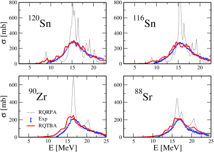
Figure 1: Total dipole photoabsorption cross section in stable medium-mass nuclei, see text for explanation.

Fragmentation of the giant dipole resonance (GDR) due to the QVC is one of the most famous phenomena in nuclear structure physics. To describe the GDR, one has to calculate the strength function of Eq. (46) as a response to an electromagnetic dipole operator which in the long wavelength limit reads:

$$P^{EM}_{1M}=\frac{N}{A}\sum\limits_{p=1}^{Z}r_{p}Y_{1M}(\Omega_{p})-\frac{Z}{A}\sum\limits_{n=1}^{N}r_{n}Y_{1M}(\Omega_{n}).$$ (47)

The cross section of the total dipole photoabsorption is given by:

$$\sigma_{E1}=\frac{16\pi^{3}e^{2}}{9{\hbar}c}ES(E).$$ (48)

Fig. 1 shows the cross sections of the total dipole photoabsorption in four medium-mass spherical nuclei obtained within the RQRPA (black dashed curves) and RQTBA (red solid curves), compared to neutron data (blue error bars) from Ref. [35]. The details of these calculations are described in Ref. [16]. One can clearly see that the QVC included within the RQTBA provides a sizable fragmentation of the GDR. The QVC mechanism of the GDR width formation is known for decades, see Refs. [36, 37, 38] and references therein. However, the RQTBA is the first fully self-consistent approach which, in contrast to the previously developed ones, accurately reproduces the Lorentzian-like GDR distribution observed in experiments.

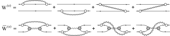
Figure 2: The 2q$\otimes$phonon amplitude $W^{(e)}$ of the conventional QVC model and the two-phonon amplitude $\bar{W}^{(e)}$ of the two-phonon model in a diagrammatic representation. The solid lines are the four-component fermion propagators, the wavy curves denote phonon propagators, the empty circles represent phonon vertices, and the grey circles together with the two nucleonic lines denote the RQRPA transition densities.

The main assumption of the RQTBA discussed so far is that two types of elementary excitations - two-quasiparticle (2q) and vibrational modes - are coupled in such a way that configurations of 2q$\otimes$phonon type with low-lying phonons strongly compete with simple 2q configurations close in energy. There are, however, additional processes, which are not fully included in this scheme as, for instance, the coupling of low-lying collective phonons to multiphonon configurations. Therefore, recently an extension of the RQTBA has been introduced, which includes also the coupling to two-phonon states [17]. In the diagrammatic representation of the amplitude $W^{(e)}$ of Eq. (42) in the upper line of the Fig. 2 the intermediate two-quasiparticle propagator is represented by the two straight nucleonic lines between the circles denoting the amplitudes of emission and absorption of the phonon by a single quasiparticle (the last term of Eq. (42) is omitted because it represents the ’compensating’ contribution [38, 34]). In the two-phonon RQTBA-2 we introduce the RQRPA correlations into the intermediate two-quasiparticle propagator replacing the amplitude $W^{(e)}$ by the new one ${\bar{W}}^{(e)}$.

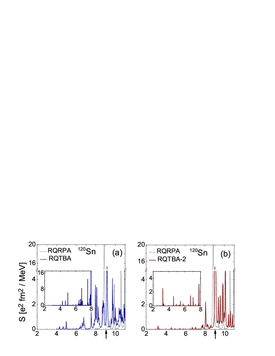
Figure 3: Low-lying dipole spectra of ¹²⁰Sn calculated within the RQRPA (dashed curves), RQTBA (blue solid curve (a)) and RQTBA-2 (red solid curve (b)). A finite smearing parameter $\Delta$ = 20 keV has been used in the calculations. The inserts show the zoomed pictures of the spectra below 8 MeV with a small value $\Delta$ = 2 keV allowing to see all the states in this energy region. The arrows indicate the neutron threshold.

Fig. 3 illustrates the effect of two-phonon correlations on spectra of nuclear excitations. It displays the dipole strength functions for ¹²⁰Sn calculated within the conventional RQTBA and the two-phonon RQTBA-2. The resulting strength functions are compared with the RQRPA strength function because both of them originate from the RQRPA by similar fragmentation mechanisms. The major fraction of the RQRPA state at the neutron threshold (pygmy mode) shown by the dashed curve is pushed up above the neutron threshold by the RQTBA-2 correlations. The lowest 1^- state, being a member of the $[2^{+}\otimes 3^{-}]$ quintuplet, appears at 3.23 MeV with B(E1)$\uparrow$ = 15.9$\times$10^-3 e² fm². These numbers can be compared with the corresponding data for the lowest 1^- state: it is observed at 3.28 MeV with B(E1)$\uparrow$ = 7.60(51)$\times$10^-3 e² fm², [39] and B(E1)$\uparrow$ = 11.20(11)$\times$10^-3 e² fm² [40]. The obtained agreement with the data is very good in spite of the fact that these tiny structure at about 3 MeV originate by the splitting-out from the very strong RQRPA pygmy state located at the neutron threshold, due to the two-phonon correlations included consistently without any adjustment procedures. The physical content of the two-phonon RQTBA reminds the two-phonon quasiparticle-phonon model [37], however, one-to-one correspondence has not been established. Also, the obtained differences between the RQTBA and RQTBA-2 results may occur because of their limitations in terms of the configuration space. Both 2q$\otimes$phonon and phonon$\otimes$phonon configurations are limited by only four quasiparticles and, perhaps, on the higher level of the configuration complexity involving six and more quasiparticles the differences between the coupling schemes will be less pronounced. This is supposed to be clarified in the future studies.

6 Outlook

The old concept of the quasiparticle-vibration coupling has been implemented on a contemporary basis: as self-consistent extensions of the relativistic QRPA built on the covariant energy density functional. In these extensions, the QVC and pairing correlations are taken into account on the equal footing while the CEDF+BCS approach provides a convenient working basis for the treatment of the complicated many-body dynamics. Applications to various nuclear structure phenomena in ordinary and exotic nuclei illustrate that the self-consistent implementation of many-body correlations beyond the CEDF theory represents a successful strategy toward a universal and precise approach for the low-energy nuclear dynamics.

References

- 1. J. Bardeen, L.N. Cooper, J.R. Schrieffer, Phys. Rev. 106, 162 (1957).
- 2. A. Bohr, B.R. Mottelson, and D. Pines, Phys. Rev. 110, 936 (1958).
- 3. P. Ring and P. Schuck, The nuclear many-body problem (Springer, Heidelberg, 1980).
- 4. V.G. Soloviev, Nucl. Phys. 9, 655 (1958/59).
- 5. S.T. Belyaev, Mat. Fys. Medd. Dan. Vid. Selsk. 31, No. 11 (1959).
- 6. N.N. Bogoliubov, Sov. Phys. JETP 7, 245 (1958).
- 7. D. Bohm and D. Pines, Phys. Rev. 92, 609 (1953).
- 8. N.N. Bogoliubov, Sov. Phys. Usp. 2, 236 (1959).
- 9. M. Baranger, Phys. Rev. 120, 957 (1960).
- 10. V.G. Soloviev, Theory of Complex Nuclei (Nauka, Moscow, 1971).
- 11. A. Gade, T. Glasmacher, Progr. Part. Nucl. Phys. 60, 161 (2008).
- 12. T. Aumann, Nucl. Phys. A 805, 198c (2008).
- 13. N. Paar, P. Ring, T. Nikšić, and D. Vretenar, Phys. Rev. C 67, 034312 (2003).
- 14. D. Vretenar, A.V. Afanasjev, G.A. Lalazissis, and P. Ring, Phys. Rep. 409, 101 (2005).
- 15. P. Ring, Prog. Part. Nucl. Phys. 37, 193 (1996).
- 16. E. Litvinova, P. Ring, and V.I. Tselyaev, Phys. Rev. C 78, 014312 (2008).
- 17. E. Litvinova, P. Ring, and V. Tselyaev, Phys. Rev. Lett. 105, 022502 (2010).
- 18. E. Litvinova, Phys. Rev. C 85, 021303 (2012).
- 19. A.A. Abrikosov, L.P. Gorkov, and I.E. Dzyaloshinski, Methods of Quantum Field Theory in Statistical Physics (Prienice-Hall, Englewood Cliffs, NJ, 1963)(Dover, New York, 1975).
- 20. J.G. Valatin, Phys. Rev. 122, 1012 (1961).
- 21. J.D. Walecka, Ann. Phys. (N.Y.) 83, 491 (1974).
- 22. B.D. Serot and J.D. Walecka, Adv. Nucl. Phys. 16, 1 (1986).
- 23. J. Boguta and A.R. Bodmer, Nucl. Phys. A 292, 413 (1977).
- 24. K. Capelle and E.K.U. Gross, Phys. Rev. B 59, 7140 (1999).
- 25. H. Kucharek and P. Ring, Z. Phys. A 339, 23 (1991).
- 26. M. Serra and P. Ring, Phys. Rev. C 65, 064324 (2002).
- 27. M.N. Harakeh, A. van der Woude, Giant Resonances: Fundamental High-Frequency Modes of Nuclear Excitation (Oxford University Press, USA, 2001).
- 28. A.B. Migdal, Theory of Finite Fermi Systems and Applications to Atomic Nuclei (Interscience, New York, 1967).
- 29. P. Ring, Z.-Y. Ma, N. Van Giai, D. Vretenar, A. Wandelt, and L.-G. Cao, Nucl. Phys. A 694, 249 (2001).
- 30. A. Bohr and B. Mottelson, Nuclear Structure (Benjamin, Reading, Mass., 1975), Vol. II.
- 31. E. Litvinova and P. Ring, Phys. Rev. C 73, 044328 (2006).
- 32. E. Litvinova, Phys. Rev. C 85, 021303(R) (2012).
- 33. E.E. Salpeter, H.A. Bethe, Phys. Rev. 84, 1232 (1951).
- 34. V.I. Tselyaev, Phys. Rev. C 75, 024306 (2007).
- 35. Experimental Nuclear Reaction Data (EXFOR), http://www-nds.iaea.org/exfor/exfor.htm
- 36. P.F. Bortignon, R.A. Broglia, D.R. Bes, and R. Liotta, Phys. Rep. 30, 305 (1977).
- 37. V. G. Soloviev, Theory of Atomic Nuclei: Quasiparticles and Phonons (Institute of Physics, Bristol and Phyladelphia, USA, 1992).
- 38. S.P. Kamerdzhiev, J. Speth, and G.Y. Tertychny, Phys. Rep. 393, 1 (2004).
- 39. J. Bryssinck et al., Phys. Rev. C 59, 1930 (1999).
- 40. B. Özel et al., Nucl. Phys. A 788, 385 (2007).