Simulation of light propagation in thin semiconductor films with non-local electron-photon interaction

Abstract

The propagation of light in layered semiconductor media is described theoretically and simulated numerically within the framework of the non-equilibrium Green’s function formalism as used for state-of-the-art nanodevice simulations, treating the non-local interaction of leaky photonic modes with the electronic states of thin semiconductor films on a non-equilibrium quantum statistical mechanics level of theory. For a diagonal photon self-energy corresponding to local coupling, the simulation results for a 500 nm GaAs slab under normal incidence are in excellent agreement with the predictions from the conventional transfer matrix method. The deviations of the local approximation from the result provided by the fully non-local photon self-energy for a 100 nm GaAs film are found to be small.

IEK5-Photovoltaik, Forschungszentrum Jülich,
D-52425 Jülich, Germany

u.aeberhard@fz-juelich.de

(250.0250) Optoelectronics; (270.0270) Quantum optics; (270.5580) Quantum electrodynamics; (310.0310) Thin films.

1 Introduction

Many novel architectures for opto-electronic devices such as solar cells or light emitting diodes utilize nanostructures as functional components for enhanced device performance. These nanoscale components interact with the electromagnetic radiation on a length scale in the sub-wavelength regime. In these devices, complex combinations of dielectric and electronic nanostructures lead to an intricate pattern of interaction of leaky photonic modes with confined electronic states. While adequate descriptions of electronic transport in structures with strong spatial inhomogeneity at the nanoscale, such as the non-equilibrium Green’s function formalism (NEGF) [1], are well established and routinely used, the consideration of the interaction of charge carriers with photon modes is in most cases still based on the local coupling to classical solutions of Maxwell’s equations. In order to fully account for electronic coherence and optical confinement in the description of the electron-photon interaction for photocurrent generation, a non-local theory of photon modes in optically open devices is required, which is compatible with the description of charge carrier transport.

In this paper, such a description is provided based on the photon Green’s functions (GF) for general non-equilibrium conditions and one dimensional spatial composition variation of the optically active medium. After a brief review of the general NEGF theory of optical modes, the steady-state equations are formulated for a semiconductor slab system and subsequently solved numerically for normal incidence of polychromatic light and both local and non-local coupling to the electronic system.

2 NEGF formalism for optical modes

The optical NEGF problem of slab systems has been discussed in the literature for several different applications, such as emission enhancement in microcavity lasers [2], absorption-reflection set-up for a general non-equilibrium system [3, 4, 5] or the photovoltaic response of a spatially homogeneous (bulk) absorber and in absence of recombination losses [6]. Here, the focus is on the absorption of external radiation that is coupled into the same leaky modes that are responsible fo the emission of light leading to radiative dark current. This treatment is required for a consistent microscopic theory of nanostructure based solar cell devices [7, 8], in which the electron-photon coupling responsible for photocarrier generation is described in terms of a self-energy including the (non-local) GFs of both charge carriers and photons.

2.1 Photon Green’s function

The photon GF can be defined via Maxwell’s equation for the effective vector potential of the electromagnetic field $\mathbf{A}_{eff}(\underline{1})\equiv\langle\hat{\mathbf{A}}(\underline{1})\rangle_{C}$ ($\underline{1}\equiv\{\mathbf{r}_{1},\underline{t}_{1}\in C\}$, $C$: Keldysh contour [9]), which can be written as a free field expansion in terms of bosonic operators,

$$\hat{\mathbf{A}}({\mathbf{r}},\underline{t})= \sum_{\lambda,{\mathbf{q}}}\left[\mathbf{A}_{0}(\lambda,\mathbf{q})\hat{b}_{\lambda,{\mathbf{q}}}(\underline{t})e^{i{\mathbf{q}}{\mathbf{r}}}+\mathbf{A}_{0}^{*}(\lambda,\mathbf{q})\hat{b}_{\lambda,{\mathbf{q}}}^{\dagger}(\underline{t})e^{-i{\mathbf{q}}{\mathbf{r}}}\right],$$ (1)

$$\mathbf{A}_{0}(\lambda,\mathbf{q})= \sqrt{\frac{\hbar}{2\epsilon_{0}V\omega_{\lambda\mathbf{q}}}}{\mathbf{\epsilon}}_{\lambda{\mathbf{q}}},$$ (2)

and induced current $\mathbf{j}_{ind}(\underline{1})\equiv\langle\hat{\mathbf{j}}(\underline{1})\rangle_{C}$, which then reads

$$\left(\Delta-\frac{n(\mathbf{r})}{c_{0}^{2}}\frac{\partial^{2}}{\partial^{2}\underline{t}}\right)\mathbf{A}_{eff}(\mathbf{r},\underline{t})=-\mu_{0}[\mathbf{j}_{ind}(\mathbf{r},\underline{t})+\mathbf{j}_{ext}(\mathbf{r},\underline{t})]$$ (3)

for an external current density $\mathbf{j}_{ext}$ (c-number function). The photon GF is then defined via the functional derivative

$$\mathcal{D}_{\mu\nu}(\underline{1},\underline{2})= -\frac{1}{\mu_{0}}\frac{\delta A_{eff,\mu}(\underline{1})}{\delta j_{ext,\nu}(\underline{2})}$$ (4)

$$= -\frac{1}{\mu_{0}}\frac{i}{\hbar}\left[\langle\hat{A}_{\mu}(\underline{1})\hat{A}_{\nu}(\underline{2})\rangle_{C}-A_{eff,\mu}(\underline{1})A_{eff,\nu}(\underline{2})\right],$$ (5)

where $\mu_{0}=1/(\varepsilon_{0}c_{0}^{2})$ is the magnetic vacuum permeability. Similarly, the transverse polarization function corresponding to the photon self-energy is defined via

$$\Pi_{\mu\nu}(\underline{1},\underline{2})= -\mu_{0}\frac{\delta j_{ind,\mu}(\underline{1})}{\delta A_{eff,\nu}(\underline{2})}.$$ (6)

The contour ordered photon GF follows as the solution of the corresponding Dyson equation

$$\int d3\left[\mathcal{D}_{0,\mu\beta}^{-1}(\underline{1},\underline{3})-\Pi_{\mu\beta}(\underline{1},\underline{3})\right]\mathcal{D}_{\beta\nu}(\underline{3},\underline{2})=\delta_{\parallel,\mu\nu}(\underline{1},\underline{2}),$$ (7)

where $\mathcal{D}_{0,\mu\nu}$ is the free propagator defined by

$$\mathcal{D}_{0,\mu\nu}^{-1}(\underline{1},\underline{2})=\left[\Delta_{1}-\frac{1}{c^{2}}\frac{\partial^{2}}{\partial\underline{t}_{1}^{2}}\right]\delta_{\mu\nu}\delta(\underline{1},\underline{2}),$$ (8)

and $\delta_{\parallel,\mu\nu}(\underline{1},\underline{2})=\delta(\underline{t}_{1}-\underline{t}_{2})\delta_{\parallel,\mu\nu}(\mathbf{r}_{1}-\mathbf{r}_{2})$ is the transverse delta function,

$$\delta_{\parallel,\mu\nu}(\mathbf{r}_{1}-\mathbf{r}_{2})= \delta_{\mu\nu}\delta(\mathbf{r}_{1}-\mathbf{r}_{2})+\nabla_{\mu}\nabla_{\nu}\frac{1}{4\pi|\mathbf{r}_{1}-\mathbf{r}_{2}|}$$ (9)

$$= \frac{1}{(2\pi)^{3}}\int d^{3}k\left(\delta_{\mu\nu}-\frac{k^{\mu}k^{\nu}}{k^{2}}\right)e^{i\mathbf{k}(\mathbf{r}_{1}-\mathbf{r}_{2})}.$$ (10)

The corresponding real time components of the retarded photon GF are determined via the Dyson equation

$$\int d3\left[\mathcal{D}_{0,\mu\beta}^{-1}(\underline{1},\underline{3})-\Pi_{\mu\beta}^{R}(\underline{1},\underline{3})\right]\mathcal{D}_{\beta\nu}^{R}(\underline{3},\underline{2})= \delta_{\parallel,\mu\nu}(\underline{1},\underline{2}).$$ (11)

The kinetic or Keldysh equations for the photon correlation functions read

$$\int d3\left[\mathcal{D}_{\mu\beta}^{R,-1}(\underline{1},\underline{3})\mathcal{D}_{\beta\nu}^{\lessgtr}(\underline{3},\underline{2})-\Pi_{\mu\beta}^{\lessgtr}(\underline{1},\underline{3})\mathcal{D}_{\beta\nu}^{A}(\underline{3},\underline{2})\right]= 0.$$ (12)

Finally, the photon spectral function is defined via

$$\hat{\mathcal{D}}_{\mu\nu}(\underline{1},\underline{2})=i[\mathcal{D}_{\mu\nu}^{R}(\underline{1},\underline{2})-\mathcal{D}_{\mu\nu}^{A}(\underline{1},\underline{2})].$$ (13)

In analogy to the electronic case, we define the local photonic density of states at steady-state ($t_{1}-t_{2}=\tau\rightarrow E$) via

$$\mathcal{N}(\mathbf{r};E)=\frac{\mathcal{C}}{2\pi}\mathrm{Tr}\{\hat{\boldsymbol{\mathcal{D}}}(\mathbf{r},\mathbf{r};E)\}$$ (14)

where the normalization factor $\mathcal{C}=\mu_{0}/(A_{0}^{2}V)=2E/(\hbar c_{0})^{2}$ ($E=\hbar\omega$) takes account of the relation of the the photon spectral function to the spectral function of non-interacting bosons [10].

2.2 Quasi-1D model for layer structures

In layer structures with homogeneous transverse dimensions, the steady-state equations for the photon GFs can be simplified by using the Fourier transform of the latter with respect to transverse coordinates, i.e.,

$$\mathcal{D}_{\mu\nu}(\mathbf{r},\mathbf{r}^{\prime},E)=\frac{A}{(2\pi)^{2}}\int d^{2}q_{\parallel}\mathcal{D}_{\mu\nu}(\mathbf{q}_{\parallel},z,z^{\prime},E)e^{i\mathbf{q}_{\parallel}\cdot(\mathbf{r}_{\parallel}-\mathbf{r}^{\prime}_{\parallel})},$$ (15)

with $A$ the cross-section area. For each energy and transverse momentum vector, a separate set of equations for the GFs needs to be solved. In the case of the retarded GF, moving the free propagator to the right in Eq. (11) leads to the integral form of the Dyson equation for the dyadic form,

$$\mathcal{D}_{\mu\nu}^{R}(\mathbf{q}_{\parallel},z,z^{\prime},E)= \mathcal{D}_{0\mu\nu}^{R}(\mathbf{q}_{\parallel},z,z^{\prime},E)$$

$$+\int dz_{1}\int dz_{2}\mathcal{D}_{0\mu\alpha}^{R}(\mathbf{q}_{\parallel},z,z_{1},E)\Pi_{\alpha\beta}^{R}(\mathbf{q}_{\parallel},z_{1},z_{2},E)\mathcal{D}_{\beta\nu}^{R}(\mathbf{q}_{\parallel},z_{2},z^{\prime},E).$$ (16)

Similarly, the kinetic equation for the correlation functions becomes

$$\mathcal{D}_{\mu\nu}^{\lessgtr}(\mathbf{q}_{\parallel},z,z^{\prime},E)= \int dz_{1}\int dz_{2}\mathcal{D}_{\mu\alpha}^{R}(\mathbf{q}_{\parallel},z,z_{1},E)\Big{[}\Pi_{0\alpha\beta}^{\lessgtr}(\mathbf{q}_{\parallel},z_{1},z_{2},E)$$

$$+\Pi_{\alpha\beta}^{\lessgtr}(\mathbf{q}_{\parallel},z_{1},z_{2},E)\Big{]}\mathcal{D}_{\beta\nu}^{A}(\mathbf{q}_{\parallel},z_{2},z^{\prime},E),$$ (17)

where the self-energy components related to the solution of the homogeneous problem, i.e., incident fluctuations that are independent from the state of the absorber, are given by [6, 3]

$$\Pi_{0\mu\nu}^{\lessgtr}(\mathbf{q}_{\parallel},z,z^{\prime},E)=\int dz_{1}\int dz_{2}[\mathcal{D}_{0}^{R}]^{-1}_{\mu\alpha}(\mathbf{q}_{\parallel},z,z_{1},E)\mathcal{D}_{0\alpha\beta}^{\lessgtr}(\mathbf{q}_{\parallel},z_{1},z_{2},E)[\mathcal{D}_{0}^{A}]^{-1}_{\beta\nu}(\mathbf{q}_{\parallel},z_{2},z^{\prime},E)$$ (18)

in terms of the GFs of the unperturbed system.

In the case of a one-dimensional dielectric perturbation potential (i.e., a 1D photonic crystal), the unperturbed GFs $\mathcal{D}_{0}$ can be defined on the basis of solutions for a homogeneous free space, which in the general case are given by (see App. A)

$$\mathcal{D}_{0\mu\nu}(\mathbf{q},E)=\frac{\hbar c_{0}^{2}}{2V}\sum_{\lambda}\frac{{\mathbf{\epsilon}}_{\lambda{\mathbf{q}}}^{\mu}{\mathbf{\epsilon}}_{\lambda{\mathbf{q}}}^{\nu}}{\omega_{\lambda\mathbf{q}}}D_{0\lambda}(\mathbf{q},E),$$ (19)

where $D_{0}$ is the scalar GF of non-interacting bosons. In the case of a homogeneous medium (e.g., vacuum), the retarded component of the free GF does not depend on polarization, and the polarization sum can be performed explicitly,

$$\sum_{\lambda}\epsilon^{\mu}_{\lambda{\mathbf{q}}}\epsilon^{\nu}_{\lambda{\mathbf{q}}}=\delta^{\mu\nu}-\frac{q^{\mu}q^{\nu}}{q^{2}}\equiv\delta^{\parallel}_{\mu\nu}(\mathbf{q}),$$ (20)

where $\delta^{\parallel}(\mathbf{q})$ is the transverse delta function in reciprocal space as given in Eq. (10). The same applies to the correlation functions, if the occupation of the modes is polarization independent, such as in the case of unpolarized incident light or completely isotropic internal emission.

The polarization-averaged GFs in slab representation are then obtained via inverse Fourier transform. Inserting the explicit forms for the GF components of non-interacting bosons in homogeneous systems (bulk) yields the expressions ($V=A\cdot L$)

$$\mathcal{D}^{R}_{0\mu\nu}(\mathbf{q}_{\parallel},z,z^{\prime},E)= \frac{\hbar^{2}c_{0}^{2}}{A}\int\frac{dq_{z}}{2\pi}\delta^{\parallel}_{\mu\nu}(\mathbf{q})e^{iq_{z}(z-z^{\prime})}\left[(E+i\eta)^{2}-(\hbar\omega_{q})^{2}\right]^{-1},$$ (21)

$$\mathcal{D}^{\lessgtr}_{0\mu\nu}(\mathbf{q}_{\parallel},z,z^{\prime},E)= -\frac{i\hbar^{2}c_{0}^{2}}{2A}\int dq_{z}\delta^{\parallel}_{\mu\nu}(\mathbf{q})e^{\pm iq_{z}(z-z^{\prime})}(\hbar\omega_{q})^{-1}$$

$$\times\Big{[}N^{0}_{{\mathbf{q}}}\delta(E\mp\hbar\omega_{q})+(N^{0}_{-{\mathbf{q}}}+1)\delta(E\pm\hbar\omega_{q})\Big{]},$$ (22)

where $q=|\mathbf{q}|=\sqrt{q_{\parallel}^{2}+q_{z}^{2}}$ and $\hbar\omega_{q}=\frac{c_{0}}{n_{0}}\hbar q$. Due to the $\mathbf{q}$-dependence of $\delta^{\parallel}$, the free GF can be separated in isotropic and anisotropic contributions,

$$\mathcal{D}_{0\mu\nu}=\mathcal{D}^{(1)}_{0}\delta_{\mu\nu}+\mathcal{D}^{(2)}_{0\mu\nu}.$$ (23)

In the case of the retarded component, further evaluation requires consideration of the polarization components. The scalar isotropic term (corresponding to the Huygens propagator) is obtained as

$$\mathcal{D}^{R(1)}_{0}(\mathbf{q}_{\parallel},z,z^{\prime},E) =-\frac{in_{0}^{2}}{2A}\frac{\exp\left[iq_{z0}(q_{\parallel},E)|z-z^{\prime}|\right]}{q_{z0}(q_{\parallel},E)},$$ (24)

where $q_{z0}(q_{\parallel},E)=\sqrt{q_{0}^{2}-q_{\parallel}^{2}}$ with $q_{0}=\frac{n_{0}}{\hbar c_{0}}|E|$. Including the full anisotropy corresponds to the consideration dyadic propagator [11]

$$\mathcal{D}^{R}_{0}(\mathbf{q}_{\parallel},z,z^{\prime},E)= -\frac{in_{0}^{2}}{2A}\frac{\exp\left[iq_{z0}(q_{\parallel},E)|z-z^{\prime}|\right]}{q_{z0}(q_{\parallel},E)q_{0}^{2}}\Big{\{}q_{0}^{2}\mathbbm{1}-\mathbf{q}_{\parallel}\otimes\mathbf{q}_{\parallel}-[q_{z0}(q_{\parallel},E)]^{2}\mathbf{\hat{z}}\otimes\mathbf{\hat{z}}$$

$$-\left(\mathbf{q}_{\parallel}\otimes\mathbf{\hat{z}}+\mathbf{\hat{z}}\otimes\mathbf{q}_{\parallel}\right)[q_{z0}(q_{\parallel},E)]^{2}\mathrm{sgn}(z-z^{\prime})\Big{\}}.$$ (25)

In the above expression, the first term in the curly bracket is the isotropic part $\mathcal{D}^{R(1)}_{0}$, while the remaining terms constitute the anisotropic part $\mathcal{D}^{R(2)}_{0}$. In the evaluation of the correlation function for free-field modes, the directional dependence of the occupation number needs to be considered. Transforming the $\delta$-function in the energy domain to the corresponding expression in terms of $q_{z}$ results in (for $E>0$ and omitting the momentum and energy dependence of $q_{z0}$ for clarity)

$$\mathcal{D}^{<}_{0\mu\nu}(\mathbf{q}_{\parallel},z,z^{\prime},E) =-\frac{in_{0}^{2}}{2A}\sum_{\sigma=+,-}\delta^{\parallel}_{\mu\nu}(\mathbf{q}_{\parallel},q_{z0\sigma})\exp[iq_{z0\sigma}(z-z^{\prime})]q_{z0}^{-1}N^{0}_{\mathbf{q}_{\parallel},q_{z0\sigma}},$$ (26)

$$\mathcal{D}^{>}_{0\mu\nu}(\mathbf{q}_{\parallel},z,z^{\prime},E) =-\frac{in_{0}^{2}}{2A}\sum_{\sigma=+,-}\delta^{\parallel}_{\mu\nu}(\mathbf{q}_{\parallel},q_{z0\sigma})\exp[-iq_{z0\sigma}(z-z^{\prime})]q_{z0}^{-1}(N^{0}_{-\mathbf{q}_{\parallel},-q_{z0\sigma}}+1),$$ (27)

where $q_{z0\sigma}=\sigma q_{z0}$.

2.3 Photon self-energy

For a simple 1D dielectric potential, the retarded photon self-energy reduces to the diagonal term $\Pi_{\mu\nu}(\mathbf{q}_{\parallel}=0,z,z^{\prime},E)=V(z,E)\delta_{\mu\nu}\delta(z-z^{\prime})$, where the dielectric potential is given by

$$V(z,E)=-\big{[}n(z,E)^{2}-n_{0}^{2}\big{]}q_{0}^{2},$$ (28)

with $n(z,E)$ the spatially varying refractive index at given photon energy, while $n_{0}$ and $c_{0}$ are refractive index and speed of light in vacuum. The effect of photon absorption can be considered for both local and non-local interaction. In the local case, the refractive index in the expression for the perturbation potential entering the diagonal photon self-energy is replaced by a complex value including the extinction coefficient $\kappa$: $n(z,E)=n_{r}(z,E)+i\kappa(z,E)$. For the consideration of the non-local interaction as mediated, e.g., by the electron-photon self-energy within the NEGF formalism of photogeneration [12], the full photon self-energy needs to be evaluated,

$$\Pi_{\mu\nu}^{\alpha}(\mathbf{q}_{\parallel},z,z^{\prime},E)=-i\hbar\mu_{0}\Big{(}\frac{e}{m_{0}}\Big{)}^{2}p_{cv}^{\mu*}(z)\mathcal{P}_{cv}^{\alpha}(\mathbf{q}_{\parallel},z,z^{\prime},E)p_{cv}^{\nu}(z^{\prime}),\qquad\alpha=\lessgtr,R,$$ (29)

where $\mathbf{p}_{cv}$ is the (local) momentum matrix and the interband polarization function is given by

$$\mathcal{P}_{cv}^{\gtrless}(\mathbf{q}_{\parallel},z,z^{\prime},E)= A^{-1}\sum_{\mathbf{k}_{\parallel}}\int\frac{dE^{\prime}}{2\pi\hbar}G_{cc}^{\gtrless}(\mathbf{k}_{\parallel},z,z^{\prime},E^{\prime})G_{vv}^{\lessgtr}(\mathbf{k}_{\parallel}-\mathbf{q}_{\parallel},z^{\prime},z,E^{\prime}-E),$$ (30)

$$\mathcal{P}_{cv}^{R}(\mathbf{q}_{\parallel},z,z^{\prime},E)= A^{-1}\sum_{\mathbf{k}_{\parallel}}\int\frac{dE^{\prime}}{2\pi\hbar}\Big{[}G_{cc}^{R}(\mathbf{k}_{\parallel},z,z^{\prime},E^{\prime})G_{vv}^{<}(\mathbf{k}_{\parallel}-\mathbf{q}_{\parallel},z^{\prime},z,E^{\prime}-E)$$

$$+G_{cc}^{<}(\mathbf{k}_{\parallel},z,z^{\prime},E^{\prime})G_{vv}^{A}(\mathbf{k}_{\parallel}-\mathbf{q}_{\parallel},z^{\prime},z,E^{\prime}-E)\Big{]}.$$ (31)

For local coupling to classical fields, the local extinction coefficient for given angle of incidence and polarization is related to the non-local photon self-energy via the local absorption coefficient [13],

$$\kappa_{\mu}(\mathbf{q}_{\parallel},z,E)=\alpha_{\mu}(\mathbf{q}_{\parallel},z,E)\cdot\frac{\hbar c_{0}}{2E}=\frac{(\hbar c_{0})^{2}}{4n_{r}E^{2}}\int dz^{\prime}\Re[i\Pi_{\mu\mu}^{>}(\mathbf{q}_{\parallel},z^{\prime},z,E)].$$ (32)

2.4 Physical quantities

Together, the different components of the photon GF provide all the spectral and integral observables that can be described in terms of single-photon operator averages. Most relevant for opto-electronic device applications such as solar cells or light emitting diodes are the local density of photon states, the local photon density and the local value of the photon flux or Poynting vector. According to (14), the general expression for the local density of photon states (LDOS) is found from the retarded GF as follows:

$$\mathcal{N}(z,E)= -\frac{\mathcal{C}}{\pi}\sum_{\mu}\sum_{\mathbf{q}_{\parallel}}\mathrm{Im}\mathcal{D}_{\mu\mu}^{R}(\mathbf{q}_{\parallel},z,z,E)\equiv\frac{\mathcal{C}}{2\pi}\sum_{\mu}\sum_{\mathbf{q}_{\parallel}}\hat{\mathcal{D}}_{\mu\mu}(\mathbf{q}_{\parallel},z,z,E).$$ (33)

The local photon density is obtained from the correlation function,

$$n_{\gamma}(\mathbf{q}_{\parallel},z,E)=\frac{\mathcal{C}}{2\pi}\sum_{\mu}i\mathcal{D}_{\mu\mu}^{<}(\mathbf{q}_{\parallel},z,z,E).$$ (34)

Finally, the $z$-component of the modal Poynting vector is given by [3]

$$s_{z}(\mathbf{q}_{\parallel},z,E)= -\frac{E}{2\pi\hbar}\lim_{z^{\prime}\rightarrow z}\partial_{z^{\prime}}\sum_{\mu}\mathrm{Re}\Big{[}\mathcal{D}_{\mu\mu}^{>}(\mathbf{q}_{\parallel},z,z^{\prime},E)+\mathcal{D}_{\mu\mu}^{<}(\mathbf{q}_{\parallel},z,z^{\prime},E)\Big{]}.$$ (35)

3 Analytical and numerical verification for normal incidence

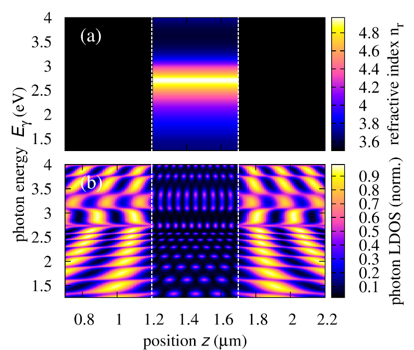
Figure 1: (a) Refractive index profile and (b) corresponding local density of photon states at vanishing transverse photon momentum $\mathbf{q}_{\parallel}=0$ for a 500 nm GaAs slab.

Figure 2: (a) Extinction coefficient $\kappa$ and (b) spectral photon flux for the AM1.5 solar spectrum under normal incidence ($\mathbf{q}_{\parallel}=0$).

As a first consistency check, the local photon density of states is computed, which in the case of free field modes should be independent of space and amount to $\mathcal{N}_{0}(z,E)=(n_{0}^{3}E^{2})/(\pi^{2}\hbar^{3}c_{0}^{3})$. Evaluating the different expressions for the diagonal polarization components for the retarded GF results in an isotropic contribution of (see App. B)

$$\mathcal{N}_{0}^{(1)}(z,E)=3\cdot\frac{n_{0}^{3}E^{2}}{2\pi^{2}\hbar^{3}c_{0}^{3}}$$ (36)

and an anisotropic contribution of

$$\mathcal{N}_{0}^{(2)}(z,E)=-\frac{n_{0}^{3}E^{2}}{2\pi^{2}\hbar^{3}c_{0}^{3}},$$ (37)

which together provides the above photon DOS of free field modes.

To verify the computation of the GF for an inhomogeneous situation and local coupling, the local photon DOS, spectral density of photons and local photon flux for a 500 nm thick GaAs slab in air are compared to the corresponding quantities as computed via a standard transfer matrix method (TMM), using the same optical data (SOPRA database) and the standard AM1.5 solar spectrum at normal incidence as external photon source. In the case of normal incidence ($\mathbf{q}_{\parallel}=0)$, the anisotropic part vanishes in $\mathcal{D}_{0}$. The corresponding integral equation for the scalar component of the retarded photon can be solved numerically either via quadrature [14] or a recursive approach [14, 15]. Due to the nonlocality of the electron-photon coupling, we adopt the former approach here, since it provides the full GF including all off-diagonal elements. It amounts to the linear problem (at fixed energy $E$)

$$\boldsymbol{\mathcal{M}}\cdot\boldsymbol{\mathcal{D}}^{R(1)}=\boldsymbol{\mathcal{D}}^{R(1)}_{0},$$ (38)

with

$$\mathcal{M}_{ij}=\delta_{ij}-\mathcal{D}_{0}^{R(1)}(z_{i},z_{j})V(z_{j}).$$ (39)

The LDOS [Fig. 1(b)] and photon density are evaluated for a real refractive index profile [Fig. 1(a)], i.e., neglecting absorption, while the photon flux [Fig. 2(b)] is computed under inclusion of the extinction coefficient [Fig. 2(a)].

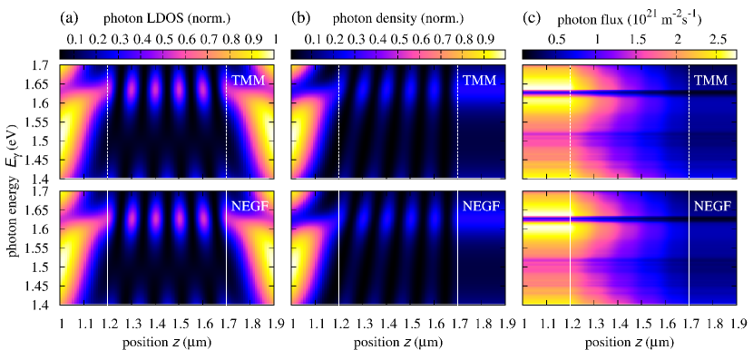
Figure 3: Comparison between the results provided by the transfer matrix method (TMM) and the non-equilibrium Green’s function formalism (NEGF) for (a) the local density of photon states at $\mathbf{q}_{\parallel}=0$, (b) the local photon density for normal incindence from the left, and (c) the local photon flux (modal Poynting vector) under illumination with the solar AM1.5g spectrum of a 500 nm GaAs slab.

For the LDOS, the NEGF expression (33) is compared to the sum of the absolute value squared of the electric field for unit left and right incidence in TMM, $\mathcal{N}^{TMM}(z,E)\propto|\mathcal{E}(z,E)|^{2}E^{2}$ [Fig. 3(a)], with normalization to the maximum value. In the regions left and right of the semiconductor slab, the numerical value of the LDOS at $q_{\parallel}=0$ approaches that of the analytical expression $\mathcal{N}_{0}^{(1)}(q_{\parallel}=0,z,E)=n_{0}/\left(\pi\hbar c_{0}A\right)$ for homogeneous bulk, which is reproduced exactly for a constant real index of refraction. For the photon density, the numerical value of expression (34) with the correlation function resulting from the solution of (17) under the assumption of an asymmetric mode occupation $N_{\mathbf{q}}=\tilde{N}(E)\delta(q_{\parallel})\theta(q_{z})$ is compared to the absolute value of the electric field for left incidence in TMM [Fig. 3(b)], again normalized to the maximum value. The decay of the photon mode occupation is monitored via the Poynting vector. Using the expression for the non-interacting GFs (26) and (27) at $\mathbf{q}_{\parallel}=0$ in (35) fixes the mode occupation $\tilde{N}(E)$ for a given incident photon flux: for normal incidence from the left, the only non-vanishing components of the correlation functions for $E>0$ are

$$\mathcal{D}_{0\mu\mu}^{<}(\mathbf{0},z,z^{\prime},E)= -\frac{in_{0}^{2}}{2A}\exp[iq_{0}(z-z^{\prime})]q_{0}^{-1}\tilde{N}(E),$$ (40)

$$\mathcal{D}^{>}_{0\mu\mu}(\mathbf{0},z,z^{\prime},E)= \frac{in_{0}^{2}}{2A}\Big{\{}\exp[iq_{0}(z-z^{\prime})]\tilde{N}(E)+2\cos[q_{0}(z-z^{\prime})]\Big{\}}q_{0}^{-1},\qquad\mu=x,y.$$ (41)

The second term in $\mathcal{D}^{>}_{0}$ originates from spontaneous emission due to vacuum fluctuations. However, this term gives no contribution to the Poynting vector, since it is entirely imaginary. The remaining expression then amounts to

$$s_{z}(\mathbf{q}_{\parallel},z,E)= -\frac{E}{2\pi\hbar}\lim_{z^{\prime}\rightarrow z}\partial_{z^{\prime}}\Big{\{}\frac{n_{0}^{2}}{A}\sin[q_{0}(z-z^{\prime})]\tilde{N}(E)\Big{\}}=\frac{n_{0}^{2}E}{2\pi\hbar A}\tilde{N}(E).$$ (42)

In terms of the incident modal intensity $s_{0z}$ (with units of photon flux), the mode occupation is thus given by

$$\tilde{N}(E)=\frac{s_{0z}(E)2\pi\hbar A}{n_{0}^{2}|E|}$$ (43)

Fig. 3(c) shows the numerical values for a photon flux corresponding to the fraction of the AM1.5g solar spectrum in the range 1.4-1.7 eV. For all the cases compared, and inspite of the NEGF being a numerical method while the TMM is semi-analytical, the accuracy is remarkable.

Finally, the light propagation for non-local coupling is compared to that for local coupling. For the description of the non-local response of the semiconductor slab, the expression (29) for the photon self-energy is evaluated using the analytical form of the slab GF for a two-band effective mass model of a homogeneous semiconductor. Only the imaginary part of the retarded and greater self-energy components is used, and, for a more realistic description, the real refractive index profile is substituted for the diagonal entries of the real part of the self-energy; also, the self-energy is assumed to be diagonal in the polarization index. Fig. 4(a) shows the corresponding local extinction coefficient according to (32) for a 100 nm slab in the energy range 1.4-1.5 eV, while the photon flux computed using the fully non-local photon self-energy is given in Fig. 4(b), together with the TMM result for the photon flux obtained with this local extinction coefficient using a spatial average $\bar{\kappa}=(z_{max}-z_{0})^{-1}\int_{z_{0}}^{z_{max}}dz\kappa(z)$. As can be inferred from these results, the approximation of local coupling tends to slightly underestimate the overall absorption, however, the deviation is in the range of the inaccuracy due to the numerical solution of equations (16) and (17).

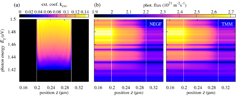
Figure 4: (a) Local extinction coefficient $\kappa(z)$ from the spatial average of the non-local photon self-energy, (b) $z$-component of the modal Poynting vector from NEGF with non-local coupling via the full self-energy and from the TMM with a spatially averaged extinction coefficient.

4 Conclusions

In this paper, a theoretical description and numerical solution of the equations governing the propagation of light in layered media was provided on the level of quantum statistical mechanics for an arbitrary non-equilibrium steady state and non-local coupling between photonic modes and electronic states. The formalism was extensively verified for normal incidence on homogeneous slab systems with spatially averaged local electron-photon interaction, finding excellent agreement with the results provided by the conventional semi-analytical transfer matrix method. Application of the formalism to the case of fully non-local coupling revealed only a minimal deviation from the predictions of the local approximation.

Appendix

Appendix A Noninteracting GF

The special case of the free photon GF for homogeneous bulk in equilibrium is described by

$$\mathcal{D}_{0\mu\nu}(1,2)=\sum_{\mathbf{q}}e^{i\mathbf{q}(\mathbf{r}_{1}-\mathbf{r}_{2})}\mathcal{D}_{0\mu\nu}(\mathbf{q};t_{1},t_{2}),$$ (44)

with

$$\mathcal{D}_{0\mu\nu}(\mathbf{q};t,t^{\prime})= \frac{\hbar c_{0}^{2}}{2V}\sum_{\lambda}(\omega_{\lambda\mathbf{q}})^{-1}\Big{[}{\mathbf{\epsilon}}_{\lambda{\mathbf{q}}}^{\mu}{\mathbf{\epsilon}}_{\lambda{\mathbf{q}}}^{\nu}D_{0\lambda}^{{}^{\prime}}(\mathbf{q};t,t^{\prime})+{\mathbf{\epsilon}}_{\lambda(-{\mathbf{q}})}^{\mu}{\mathbf{\epsilon}}_{\lambda(-{\mathbf{q}})}^{\nu}D_{0\lambda}^{{}^{\prime\prime}}(-\mathbf{q};t,t^{\prime})\Big{]}$$

$$= \frac{\hbar c_{0}^{2}}{2V}\sum_{\lambda}\frac{{\mathbf{\epsilon}}_{\lambda{\mathbf{q}}}^{\mu}{\mathbf{\epsilon}}_{\lambda{\mathbf{q}}}^{\nu}}{\omega_{\lambda\mathbf{q}}}\Big{[}D_{0\lambda}^{{}^{\prime}}(\mathbf{q};t,t^{\prime})+D_{0\lambda}^{{}^{\prime\prime}}(-\mathbf{q};t,t^{\prime})\Big{]}$$ (45)

$$\equiv \frac{\hbar c_{0}^{2}}{2V}\sum_{\lambda}\frac{{\mathbf{\epsilon}}_{\lambda{\mathbf{q}}}^{\mu}{\mathbf{\epsilon}}_{\lambda{\mathbf{q}}}^{\nu}}{\omega_{\lambda\mathbf{q}}}D_{0\lambda}(\mathbf{q};t,t^{\prime}),$$ (46)

where the bare scalar photon (boson) propagator is defined as

$$D_{0\lambda}(\mathbf{q};t,t^{\prime})\equiv -\frac{i}{\hbar}\left\langle\hat{T}_{C}\left\{[\hat{b}^{\dagger}_{\lambda,-\mathbf{q}}(t)+\hat{b}_{\lambda,\mathbf{q}}(t)][\hat{b}^{\dagger}_{\lambda,\mathbf{q}}(t^{\prime})+\hat{b}_{\lambda,-\mathbf{q}}(t^{\prime})]\right\}\right\rangle_{0}$$ (47)

$$= -\frac{i}{\hbar}\left[\left\langle\hat{T}_{C}\left\{\hat{b}_{\lambda,\mathbf{q}}(t)\hat{b}^{\dagger}_{\lambda,\mathbf{q}}(t^{\prime})\right\}\right\rangle_{0}+\left\langle\hat{T}_{C}\left\{\hat{b}^{\dagger}_{\lambda,-\mathbf{q}}(t)\hat{b}_{\lambda,-\mathbf{q}}(t^{\prime})\right\}\right\rangle_{0}\right].$$ (48)

The corresponding real-time steady-state expressions are

$$D_{0\lambda}^{\lessgtr}({\mathbf{q}},E) =-2\pi i\left[N^{0}_{\lambda,{\mathbf{q}}}\delta(E\mp\hbar\omega_{\lambda{\mathbf{q}}})+(N^{0}_{\lambda,-{\mathbf{q}}}+1)\delta(E\pm\hbar\omega_{\lambda{\mathbf{q}}})\right],$$ (49)

$$D_{0\lambda}^{R,A}({\mathbf{q}},E) =\frac{1}{E-\hbar\omega_{\lambda{\mathbf{q}}}\pm i\eta}-\frac{1}{E+\hbar\omega_{\lambda{\mathbf{q}}}\pm i\eta}$$ (50)

$$=\frac{2\hbar\omega_{\lambda{\mathbf{q}}}}{(E+i\eta)^{2}-(\hbar\omega_{\lambda{\mathbf{q}}})^{2}},$$ (51)

where $\eta\rightarrow 0^{+}$ and

$$N_{\lambda,{\mathbf{q}}}^{0}\equiv \langle\hat{b}^{\dagger}_{\lambda,\mathbf{q}}\hat{b}_{\lambda,\mathbf{q}}\rangle_{0}$$ (52)

is the occupation of photon mode $(\lambda,\mathbf{q})$.

Appendix B Dyadic propagator in cylindrical coordinates

For a situation with spatial isotropy in the transverse dimensions, cylindrical coordinates can be used, where $\mathbf{q}_{\parallel}=q_{\parallel}\left(\cos\varphi,\sin\varphi\right)$, and the azimuthal dependence of the GF can be separated from the dependence on the absolute value of the transverse momentum, i.e., $\mathcal{D}_{0\mu\nu}(\mathbf{q}_{\parallel},z,z^{\prime},E)=\mathcal{D}_{0\mu\nu}(q_{\parallel},\varphi,z,z^{\prime},E)$. In this case, the full retarded GF can be written as

$$\mathcal{D}_{0\mu\nu}^{R}(q_{\parallel},\varphi,z,z^{\prime},E)=\mathcal{H}(q_{\parallel},z,z^{\prime},E)\mathcal{F}_{\mu\nu}(q_{\parallel},\varphi,z,z^{\prime},E)$$ (53)

with the scalar, angle-independent Huygens propagator

$$\mathcal{H}(q_{\parallel},z,z^{\prime},E)=-\frac{in_{0}^{2}}{2A}\frac{\exp\left[iq_{z0}(q_{\parallel},E)|z-z^{\prime}|\right]}{q_{z0}(q_{\parallel},E)}$$ (54)

and

$$\mathcal{F}_{\mu\nu}(q_{\parallel},\varphi,z,z^{\prime},E)=q_{0}^{-2}$$

$$\times\begin{pmatrix}q_{0}^{2}-q_{\parallel}^{2}f_{xx}(\varphi)&-q_{\parallel}^{2}f_{xy}(\varphi)&-q_{\parallel}q_{z0}f_{xz}(\varphi)\mathrm{sgn}(z-z^{\prime})\\ -q_{\parallel}^{2}f_{xy}(\varphi)&q_{0}^{2}-q_{\parallel}^{2}f_{yy}(\varphi)&-q_{\parallel}q_{z0}f_{yz}(\varphi)\mathrm{sgn}(z-z^{\prime})\\ -q_{\parallel}q_{z0}f_{xz}(\varphi)\mathrm{sgn}(z-z^{\prime})&-q_{\parallel}q_{z0}f_{yz}(\varphi)\mathrm{sgn}(z-z^{\prime})&q_{\parallel}^{2}\end{pmatrix},$$ (55)

where the angular factors $f_{\mu\nu}(\varphi)$ are given by

$$f_{xx}(\varphi)=\cos^{2}\varphi,~{}f_{yy}(\varphi)=\sin^{2}\varphi,~{}f_{zz}(\varphi)=1,$$ (56)

$$f_{xy}(\varphi)=\sin\varphi\cos\varphi,~{}f_{xz}(\varphi)=\cos\varphi,~{}f_{yz}(\varphi)=\sin\varphi.$$ (57)

In the continuum limit, the summation over transverse photon momentum in the expressions for LDOS [Eq. (33)] and local photon density [Eq. (34)] is replaced by integrations over absolute value of momentum and over angle,

$$\sum_{\mathbf{q}_{\parallel}}\rightarrow\frac{A}{(2\pi)^{2}}\int_{0}^{q_{0}}dq_{\parallel}q_{\parallel}\int_{0}^{2\pi}d\varphi$$ (58)

Upon the angular integration, only the diagonal terms of $\mathbf{f}$ survive ($\bar{f}_{\mu\nu}=\int d\varphi f_{\mu\nu}$):

$$\bar{f}_{xx}=\bar{f}_{yy}=\pi,\quad\bar{f}_{zz}=2\pi.$$ (59)

The angular average of the diagonal anisotropic components of the retarded GF for free field modes is thus given by

$$\bar{\mathcal{D}}_{0xx}^{R(2)}(q_{\parallel},z,z,E)= \bar{\mathcal{D}}_{0yy}^{R(2)}(q_{\parallel},z,z,E)$$ (60)

$$= -\pi q_{\parallel}^{2}q_{0}^{-2}\mathcal{H}(q_{\parallel},z,z,E)=\frac{in_{0}^{2}}{2A}\frac{\pi q_{\parallel}^{2}}{q_{z0}(q_{\parallel},E)q_{0}^{2}},$$ (61)

$$\bar{\mathcal{D}}_{0zz}^{R(2)}(q_{\parallel},z,z,E)= -2\pi q_{z0}(q_{\parallel},E)q_{0}^{-2}\mathcal{H}(q_{\parallel},z,z,E)=\frac{in_{0}^{2}}{2A}\frac{2\pi q_{z0}(q_{\parallel},E)}{q_{0}^{2}}.$$ (62)

Integration over transverse momentum und normalization with $\mathcal{C}=\frac{2E}{(\hbar c_{0})^{2}}$ provides the anisotropic DOS components via

$$\mathcal{N}_{\mu\mu}^{(2)}(z,E)= -\frac{\mathcal{C}}{\pi}\frac{A}{(2\pi)^{2}}\int_{0}^{q_{0}}dq_{\parallel}q_{\parallel}\mathrm{Im}\bar{\mathcal{D}}_{\mu\mu z}^{R(2)}(q_{\parallel},z,z,E)$$ (63)

$$= -\frac{1}{3}\frac{n_{0}^{3}E^{2}}{2\pi^{2}(\hbar c_{0})^{3}},\quad\mu=x,y,z.$$ (64)

The isotropic part of the angle-averaged diagonal retarded GF is

$$\bar{\mathcal{D}}_{0\mu\mu}^{R(1)}(q_{\parallel},z,z,E)= 2\pi\mathcal{H}(q_{\parallel},z,z,E)=-\frac{in_{0}^{2}}{2A}\frac{2\pi}{q_{z0}(q_{\parallel},E)},\quad\mu=x,y,z,$$ (65)

which provides the isotropic part of the LDOS components

$$\mathcal{N}_{\mu\mu}^{(1)}(z,E)= \frac{n_{0}^{3}E^{2}}{2\pi^{2}(\hbar c_{0})^{3}},\quad\mu=x,y,z.$$ (66)

References

• [1] S. Datta, Electronic Transport in Mesoscopic Systems (Cambridge University Press, 1995).
• [2] F. Jahnke and S. W. Koch, “Many-body theory for semiconductor microcavity lasers,” Phys. Rev. A 52, 1712–1727 (1995).
• [3] F. Richter, M. Florian, and K. Henneberger, “Generalized radiation law for excited media in a nonequilibrium steady state,” Phys. Rev. B 78, 205114 (2008).
• [4] K. Henneberger, “Generalizing planck’s law: Nonequilibrium emission of excited media,” Phys. Status Solidi B 246, 283 (2009).
• [5] K. Henneberger and F. Richter, “Exact property of the nonequilibrium photon green function for bounded media,” Phys. Rev. A 80, 013807 (2009).
• [6] D. Mozyrsky and I. Martin, “Efficiency of thin film photocells,” Opt. Commun. 277, 109 (2007).
• [7] U. Aeberhard, “Theory and simulation of quantum photovoltaic devices based on the non-equilibrium green’s function formalism,” J. Comput. Electron. 10, 394–413 (2011).
• [8] U. Aeberhard, “Simulation of nanostructure-based high-efficiency solar cells: Challenges, existing approaches, and future directions,” IEEE J. Sel. Topics in Quantum Electron. 19, 4000411 (2013).
• [9] L. Keldysh, “Diagram technique for nonequilibrium processes,” Sov. Phys. JETP 20, 1018 (1965).
• [10] P. M. Derlet, “Planck’s radiation law: a many-body perspective,” Aust. J. Phys. 49, 589 (1996).
• [11] O. Keller, Quantum Theory of Near- Field Electrodynamics, Nano-Optics and Nanophotonics (Springer, Heidelberg, 2011).
• [12] U. Aeberhard, “Quantum-kinetic theory of photocurrent generation via direct and phonon-mediated optical transitions,” Phys. Rev. B 84, 035454 (2011).
• [13] U. Aeberhard, “Quantum-kinetic theory of steady-state photocurrent generation in thin films: coherent vs. incoherent coupling,” unpublished.
• [14] K. Kahen, “Analysis of distributed-feedback lasers using a recursive green’s functional approach,” IEEE J. Quantum. Electron. 29, 368 –373 (1993).
• [15] A. I. Rahachou and I. V. Zozoulenko, “Light propagation in finite and infinite photonic crystals: The recursive green’s function technique,” Phys. Rev. B 72, 155117 (2005).