The biphase explained: understanding the asymmetries in coupled Fourier components of astronomical timeseries

Abstract

We make the first attempt to estimate and interpret the biphase data for astronomical time series. The biphase is the phase of the bispectrum, which is the Fourier domain equivalent of the three-point correlation function. The bispectrum measures two key nonlinear properties of a time series – its reversability in time, and the symmetry about the mean of its flux distribution – for triplets of frequencies. Like other Fourier methods, it is especially valuable for working with time series which contain large numbers of cycles at the period of interest, but in which the signal-to-noise at a given frequency is small in any individual cycle, either because of measurement errors, or because of the contributions from signals at other frequencies. This has long been the case for studies of X-ray binaries, but is increasingly becoming true for stellar variability (both intrinsic and due to planetary transits) in the Kepler era. We attempt in this paper also to present some simple examples to give a more intuitive understanding of the meaning of the bispectrum to readers, in order to help to understand where it may be applicable in astronomy. In particular, we give illustrative examples of what biphases may be shown by common astrophysical time series such as pulsars, eclipsers, stars in the instability strip, and solar flares. We then discuss applications to the biphase data for understanding the shapes of the quasi-periodic oscillations of GRS 1915+105 and the coupling of the quasi-periodic oscillations to the power-law noise in that system.

1 Introduction

Astronomy is one of the first sciences to make use of time series analysis, with the studies of the orbits of planets in the solar system (see e.g. Way et al. 2012 and references within for some examples). Perhaps because of the historical emphasis on orbits, astronomical time series analysis has traditonally focused on the frequencies at which the strongest variability is found, with comparitively less emphasis on the phases of different Fourier components of time series.

In a variety of systems in nature, and in laboratory studies of dynamical systems, power spectra of sources reveal strong variability over a wide range of frequencies. In order to be able to demonstrate that power exists on a large range of timescales, one ideally will have time series on which to work which are uninterrupted (or at least regularly sampled) and which are long relative to the timescales of interest. In X-ray binaries, the fast timescales of variation and strong variability allow one to probe a wide range of timescales effectively, and it has been known for about four decades that aperiodic variability can be strong in these objects (e.g. Terrell 1972). Time series of magnetograms from active regions of the Sun, which can also be made at high cadence over long time spans, also show power spectra well modelled by power laws over wide ranges of frequencies, rather than by power at a few discrete frequencies (Abramenko 2005). In recent years, the Kepler satellite has taken long, nearly uninterrupted time series of many other stars, and components in the power spectra of solar-type stars which span a broad range of frequencies have been observed (e.g. Jiang et al. 2011).

Simple tools exist for studying the time profiles of oscillations when the variability is strictly periodic (albeit, perhaps non-sinusoidal). In cases of bright sources, with variations much larger than the noise level on individual data points, one can simply examine the raw time series in the time domain. When larger noise components are present (whether they are physical, such as the noise due to stellar activity on a star with planetary transits, or are simply noise due to measurement uncertainties), one can fold the time series on the period and see the mean profile. What has generally not been done in astronomy is to examine the phase couplings of aperiodic variability.

In the cases where phase dependences are studied, often, the emphasis is on lags between different photon wavelengths (as e.g. in reverberation mapping of active galactic nuclei – e.g. Edelson & Krolik 1998 or studies of time lags in X-ray binaries – e.g. Nowak et al. 1999) – although, in some cases, some information about the nonlinearity of a system can be obtained solely through studies of the power spectrum and the cross-spectrum or cross correlation function (e.g. Maccarone, Coppi & Poutanen 2000; Shaposhnikov 2012). The reasons for this are twofold. First, under some circumstances the meaning of the phase lag between two wavelengths of light can have an immediately obvious interpretation. For example, in the case of reverberation mapping, it gives the added light travel time by taking a route that passes through the line emission region.

Secondly, making measurements of nonlinear variability in systems which possibly have red noise contributions requires a large number of high quality independent measurements of the Fourier spectrum (or some alternative statistical measure of the Fourier spectrum). This is rarely the case in astronomy. Furthermore, the real advantages of non-linearity analyses in the Fourier domain are seen when the signal-to-noise on individual measurements is poor, but a very large number of measurements exist; and/or there is substantial aperiodic variability, or there are a very large number of frequencies contributing to the variability, so that simple folding of the data on a characteristic period does not capture all that is happening in the system.

X-ray binaries represent a particularly good example of a class of systems which are particularly ripe for sophisticated nonlinearity analyses. They show variability on a wide range of timescales. They are typically the subjects of very low background rate observations where individual photons are counted and, with many X-ray observatories, the count rate per time resolution element is significantly less than unity. In recent years satellites such as Kepler and Corot have obtained very long, high precision uninterrupted observations of bright stars, which are likely to be affected by some combination of asteroseismic modes, planetary transits, coronally activity and atmospheric turbulence (e.g Jiang et al. 2011), and which also allow the study of the evolution of the rapid variability of cataclysmic variables (Scaringi et al. 2012).

There have been some attempts made to characterize and understand the nonlinear variability of X-ray binaries. In the very early era of X-ray astronomy, some attempts were made to measure, for example, the asymmetries of light curves (Priedhorsky et al.1979). More recently, that there is some nonlinearity was proved by the presence of an rms-flux relation (Uttley & McHardy 2001).

In this paper, we present a more detailed treatment than has been presented in the past of what can be learned from use of the bispectrum. Because the topic is fairly new to astronomical time series analysis, we will take a more pedagogical tone than is taken in most typical papers in astronomy, and will develop some ideas already well known in other fields of research. We will show, in particular, that the bispectrum presents a good means for determining whether a time series is reversible (in a statistical sense) and whether a time series has a symmetric flux distribution.

2 The bispectrum: a tutorial

The bispectrum is an example of a higher order time series analysis technique which can be used to understand the phase correlations in a single time series. Successful applications have been made in studies of brain waves (e.g. Gajraj et al. 1998), of speech patterns (Fackrell 1997), of vibrations of machinery (Rivola & White 1998), plasma physics (van Milligen et al. 1995), and, ocean waves, for which it was first developed (Hasselman et al. 1963). Spatial, rather than temporal, bispectra have been studied widely in astronomy, for purposes of undertanding the non-gaussianity of the cosmic microwave background (e.g. Kamionkowski et al. 2011). A large fraction of the literature on the bispectrum was developed for the study of ocean waves, and we will draw heavily on what has already been developed in that field for building up our understanding of what we can learn from the bispectrum.

The bispectrum is the first in a series of polyspectra – analogies to the classical Fourier spectrum which take into account more than one timescale. The bispectrum of two frequencies, $k$ and $l$, $B(k,l)$ is defined by:

$$B(k,l)=\frac{1}{K}\sum_{i=0}^{K-1}X_{i}(k)X_{i}(l)X^{*}_{i}(k+l),$$ (1)

where there are $K$ segments to a time series, and $X_{i}(f)$ denotes the Fourier transform of the $i$th segment of the light curve at frequency $f$. The asterisk is used in the final term to denote that a complex conjugate is being taken.

One can see that, in order to produce useful measurements of the bispectrum, one needs to have a large number of independent measurements of the time series, each with high signal to noise, and with the power spectrum stationary over the duration of the observations. The expectation value of the bispectrum is unaffected by Gaussian noise, but its value can be strongly affected by Poisson noise (e.g. Uttley et al. 2005), since Poisson noise is nonlinear.

The bispectrum is related to two quantities of a time series, the skewness and the asymmetry. The skewness is related to the mean cube of the values of the data points in a distribution in the same way that the variance is related to the mean square of the data points in a distribution – i.e. it is the third moment of the flux distribution. The asymmetry is related to the directionality of the time series, in a manner similar, but not identical, to the time skewness statistic developed by Priedhorsky et al. (1979) which is applied in the time domain and considers only a single characteristic timescale. In Maccarone & Coppi (2002), we adapted the time skewness statistic of Priedhorsky et al. (1979) by rearranging some terms and dividing by the cube of the standard deviation to non-dimensionalize the time skewness.

$$TS(\tau)=\frac{1}{\sigma^{3}}\frac{1}{K}\sum_{i=0}^{K-1}(s(t)-\bar{s})^{2}(s(t-\tau)-\bar{s})-(s(t)-\bar{s})(s(t-\tau)-\bar{s})^{2}$$ (2)

Given that the bispectrum is simply a complex number, it can be thought of as consisting of a magnitude and a phase. The phase is called the biphase, and for reasons that will become clear in the next section, the biphase must be defined over the full $2\pi$ interval, and not simply as the arctangent of the imaginary part of the bispectrum divided by the real part of the bispectrum as is sometimes done in the bispectrum literature. A version of the magnitude has been considered most heavily in previous astronomical time series papers. This version is known as the bicoherence. It is quite similar to the cross-coherence used to test whether the time lags between two energy bands are constant – it takes on a value from 0 to 1, with 0 indicating that there is no nonlinear coupling of the phases of the different Fourier components between different observations, and 1 indicating total coupling. The most commonly used expression for the bicoherence is that of Kim & Powers (1979):

$$b^{2}(k,l)=\frac{\left|\sum{X_{i}(k)X_{i}(l)X^{*}_{i}(k+l)}\right|^{2}}{\sum{\left|X_{i}(k)X_{i}(l)\right|^{2}}\sum{\left|X_{i}(k+l)\right|^{2}}},$$ (3)

where $b^{2}(k,l)$ is the squared bicoherence – although see e.g. Hinich & Wolinsky (2004) who point out that other methods of normalization are more sensitive to some types of non-linear behavior. The Kim & Powers (1979) normalization has the attractive property that, for a system with power at only three frequencies, the squared bicoherence represents the fraction of the power at the third frequency that can be explained by coupling of the three modes (see also Elgar & Guza 1985); such a simple interpretation, however, is not possible in the cases of broadband coupling (McComas & Briscoe 1980).

2.1 Understanding the biphase

The biphase thus holds powerful information about the shape of the light curve. Masuda & Kuo (1981) worked out some key implications of the biphase. In the early papers on the bispectrum (e.g. Hasselmann et al. 1963), the focus was on the skewness, which is closely related to the real part of the bispectrum. Masada & Kuo’s paper examined a few simple cases, where only three commensurate frequencies were considered, and present a few examples showing that a positive skewness when considering a particular set of timescales will manifest itself in a positive real component for the bispectrum. The real component describes the extent to which the flux distribution of the source is skewed, and the imaginary component described the extent to which the time series is symmetric in time in a statistical sense. Poisson noise thus affects only the real component.

2.1.1 Skewness of the flux distribution

A positive skewness results from an asymmetric distribution of fluxes, with a long tail to high flux. Accreting objects often show log-normal flux distributions (see e.g. Lyutyj & Oknyanskij 1987; Gaskell 2004; Uttley, McHardy & Vaughan 2005) – note also that the fact that the optical fluxes of active galactic nuclei follow a log-normal distribution is obscurred, to some extent by the use of the logarithmic magnitude scale, rather than fluxes, for most optical work (Gaskell 2004). The log-normal distribution has a positive skewness. Therefore, any cases of negative real components of bispectra (or, alternative, of biphases in the range from $\pi/2$ to $3\pi/2$) are especially interesting, as they indicate particular timescales in particular observations on which can immediately determine that the flux distribution is not the “standard” log-normal distribution.

The log-normal distribution is often found to provide a good first order description of the distribution of values of a range of phenomena, both in nature (e.g. Makuch et al. 1979), and in the social sciences (the log-normal distribution is an underlying assumption in the Black & Scholes 1973 formula for option pricing – although is has been argued to underpredict rare events – e.g. Haug & Taleb 2011). As a result, in some cases, it may make sense to apply time series analysis techniques to the logarithms of the measured values, rather than to the values themselves – in such a case finding a substantial value of the real component of the bispectrum would indicate that the distribution deviated from log-normal, which might be more enlightening than demonstrating that the distribution deviates from being symmetric about the mean. We do not make calculations of the properties of the log of the count rate distributions in this paper, but rather we simply note that it may be worth doing under certain circumstances (e.g. it may make more sense to work with magnitudes than fluxes when dealing with bright optical sources, if the optical flux distribution is expected to be log-normal).

2.1.2 Asymmetry of the time series

The asymmetry of the time series is related to the imaginary component of the bispectrum. A biphase of $\pm{\pi}/2$ is obtained for a sawtooth wave. A sawtooth wave, for example, has a symmetric flux distribution, and hence a zero real component for the bispectrum and complete asymmetry in time, and hence a purely imaginary component to the bispectrum. The sign convention is such that positive imaginary components of the bispectrum correspond to sawtooths which rise more slowly than they fall off. Again, there are some indications of what to expect from past measurements. For X-ray binaries in the hard state, for example, Maccarone, Coppi & Poutanen (2000) suggested on the basis of the combination of hard time lags and narrower autocorrelation functions at higher energies that the characteristic variability pattern for these systems must be a relatively slow rise characterized by a relatively fast fall-off, and that this slow rise must be slower and start earlier at low energies than it does at higher energies. This basic idea, at least for the rapid variability was verified by use of the time skewness statistic (Maccarone & Coppi 2002).

We note also that one can also think of the asymmetry in time as being the skewness of the Hilbert transform of the time series. The Hilbert transform, in the Fourier domain, can be executed by shifting the phases of all positive frequency components by $-90$ degree and all of the negative frequency components by $+90$ degrees. Since this converts sin $x$ to $-{\rm cos}x$, and cos $x$ to sin $x$, we can see that it bears a relation to the negative derivative of the function (although no weighting by the frequencies is applied). This thus yields some similarity with the time skewness statistic, which is a flux-weighted average of the slope of the light curve on a particular timescale.

3 Plots for extreme cases

We now present schematic diagrams for a few “extreme” cases of light curves that can occur astrophysically. These can be used to develop an intuitive picture of what lightcurves should look like for different values of the biphase.

3.1 “Ideal” pulsars: harmonics with biphase = 0

First, let us consider an overly simplified description of a pulsar light curve. If we suppose that the time series has a series of $\delta-$functions appearing periodically, where the source is bright, and has zero flux at all other times, then clearly there is no asymmetry to the time series, but there is a strong skewness in the flux distribution, with most of the data points at values much less than the mean. Such a timeseries will have a positive skewness on all timescales on which there is power in the power spectrum. The biphase will thus generically be 0 wherever there is power. For pulse shapes with some asymmetry to them, there will be biphases different from zero, but always with positive real components to the bispectrum.

3.2 Eclipses: harmonics with biphase = $\pi$

Next, we can consider the opposite case: periodic drops in flux of a constant amount which occur periodically. Apart from a DC offset and a constant of proportionality, this scenario is essentially the same as taking each flux value to be the negative of the flux values of the scenario above. This gives a strong negative skewness, and no asymmetry. The biphase should thus be $\pi$ for all cases where there is any Fourier power. The plots of time series which have biphases of 0 and $\pi$ are presented in figure 1.

Figure 1: Left: a pulsar-like time series, produced by adding cosines all with phase 0, frequencies of $j{\omega_{0}}$, where $\omega_{0}$ is the fundamental frequency of the oscillation, and $j$ are all integers. Only the first 40 terms of the sum are added, and the normalization of each component is taken to be $1/j$. Right: an eclipser-like time series, produced in the same manner as the pulsar-like time series, except that a phase of $\pi$ is added to each cosine, giving the triplets of harmonics biphases of $-\pi$.

3.3 Sawtooth oscillations: harmonics with biphase of $\pm\pi/2$

While sawtooth oscillations are not common in astrophysics, there are a few cases where they are seen. For example, solar flare radio emission can sometimes show linear rises followed by rapid drops in flux (Klassen et al. 2001) – and these sawtooth oscillations are common in other kinds of magnetic reconnection scenarios (Zweibel & Yamada 2009). Classical Cepheids and RR Lyrae stars show the opposite - sharp rises in flux, followed by slow, linear decays. Rapidly rising, linearly fading sawtooths will give $-\pi/2$ for the biphase and linearly rising, rapidly fading sawtooths will give $\pi/2$ for the biphase. Generically, any function which rises more sharply than it fades will have a negative imaginary component of the biphases and and function which fades more sharply than it rises will have a positive imaginary component of the biphase.

A strict sawtooth wave is defined as the summation over all integer values of $j$ of $\frac{1}{j}{\rm cos}[j\omega_{0}t+(j-1)\times{\pi}/2]$. The constant added phase may alternatively be multiplied by $-1$ to allow the opposite sense of symmetry. We plot the summation of the first 40 terms of a sawtooth oscillation in figure 2. As the number of terms approaches infinity, the wave form approaches a strict instantaneous rise, linear decay (or linear rise, instantaneous decay).

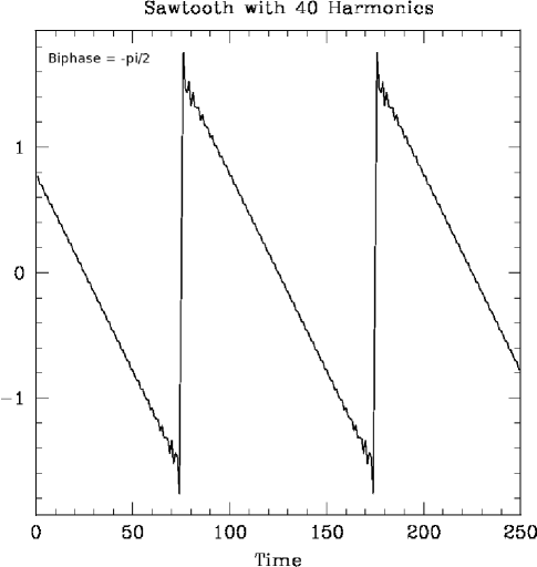
Figure 2: This is a summation of the first 40 harmonics for a sawtooth oscillation with a biphase of $-\pi/2$.

3.4 Beyond the simple examples

It is important to remember, also that the biphase alone does not determine the shape of a time series. The examples listed above are the easiest cases to visualize for their particular values of the biphase. However, these are all cases where the power spectrum is composed solely of a fundamental frequency and its overtones, and where the amplitudes of the different harmonics are set in a specific manner. In a sawtooth wave, for example, the normalization of the sine wave corresponding to a particular harmonic is inversely proportional to its frequency. A system with the same set of biphases, but a different power spectrum, would similarly be strongly asymmetric in time, but could have a light curve with a qualitatively different shape.

For example, in figure 3 we plot a modification of the sawtooth wave. Like in figure 2, we plot the sum of 40 harmonics, all as cosine waves with an added phase of $\pi/2\times(j-1)$, for the $j$th harmonic. Instead of using a normalization of $1/j$ for the Fourier spectrum, we use $1/j^{2}$, which gives more weight to the lower harmonics, and thus results in the more curved shape to the time series near the peak. The time series is still symmetric in its flux distribution, and asymmetric in time, and so it still has biphase of $-\pi/2$.

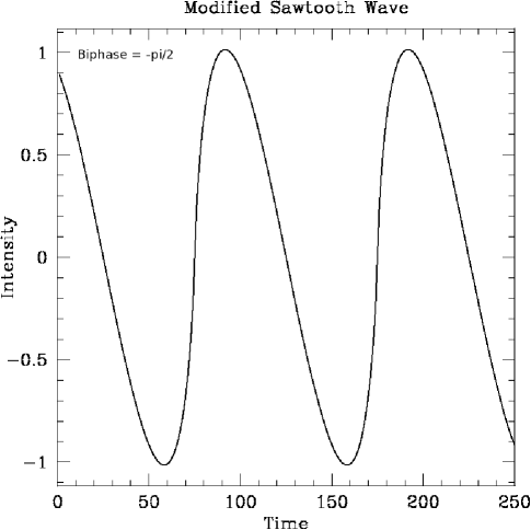
Figure 3: This is a modified sawtooth. The frequencies which contribute, and the phases at those frequencies are the same as for the sawtooth wave in figure 2, but the amplitudes of the cosine waves at the different harmonics have been changed to scale as $1/j^{2}$ instead of scaling as $1/j$. This sawtooth wave has biphase $-\pi/2$ for all combinations of harmonics in which the two lower frequencies add up to the higher frequency.

3.5 Beyond a pure harmonic structure

The easiest examples for which to attempt to visualize the bispectrum are the cases where all the relevant frequencies are integer multiples of a fundamental frequency. The real power spectra of many interesting classes of astrophysical objects, including, but not limited to, accreting compact objects with low magnetic fields, have quite broad power spectra. At the present time, it has been shown only for GRS 1915+105 that this broad power spectrum carries a nonlinear relationship with the quasi-periodic oscillations seen in the source (Maccarone et al. 2011).

Given this finding, it is of interest to show what the light curves will look like for different types of power spectra and different values of the biphase, in order to help develop an intuition for the meaning of the biphase. We thus present some calculations of simulated light curves for such Fourier spectra. We generate a Fourier spectrum using an approach similar to that taken in Timmer & König (1995) – see also Davies & Harte (1987) – with some small modifications.

First, we consider examples where the two noise components are both at lower frequencies than the QPO frequency. We draw a random amplitude at each frequency such that the power spectrum will take a value uniformly distributed between 0 and 2 times the desired power spectrum level at that frequency. We draw phases randomly for the lower non-QPO frequency, and then force the combination of the higher non-QPO frequency’s phase and the QPO frequency’s phase to give the biphase at the desired value – this forces the biphase to have a particular value for the case where $f_{1}+f_{2}=f_{QPO}$. There is then no consistent value of the biphase for the coupling within the noise component, but there is a consistent value of the biphase of the QPO.

We compute some illustrative examples of time series with different values of the biphase. We treat the noise as a power spectrum with a broken power law, with flat power below a break frequency, and a $\nu^{-1}$ slope above the break frequency. The break frequency is set to be 1/4 of the QPO frequency. The QPO is modelled as a peak at a single frequency (i.e. it is taken to be strictly periodic) for the sake of simplicity. Above the QPO frequency, we assume there is no Fourier power. We consider the cases with biphases of 0, $\pi/2$, $\pi$, and $-\pi/2$, and plot them in figure 4. We then perform the same procedure as above, except for a case where the QPO frequency is set to be about 2/3 of the break frequency of the noise power spectrum. The results of these calculations are plotted in figure 5.

The basic structures of the signals still agree with the idealized cases discussed above. When the biphase is 0, one can see that the deviations from the mean are sharper, but less frequent in the positive direction than in the negative direction, while the opposite is true for biphase of $\pi$. Furthermore, computation of the skewness of the time series yields positive values for the former case and negative values for the latter case. When the biphase is $-\pi/2$, one can see that there are sharp rises from the mean, followed by slower decays in the value of the time series, and the oppsite is true for a biphase of $\pi/2$.

Figure 4: The bispectra for the four cases where all the noise power is at lower frequencies than the QPO power. The figure in the upper left has a biphase of 0, the figure in the upper right has a biphase of $\pi$, the figure in the lower left has a biphase of $\pi/2$ and the figure in the lower right has a biphase of $-\pi/2$. The same seed was used for the random number generator for all four cases, resulting in some features dominated by the noise component looking similar in all four plots.

Figure 5: The bispectra for the four cases where QPO frequency is below the noise break frequency. The figure in the upper left has a biphase of 0, the figure in the upper right has a biphase of $\pi$, the figure in the lower left has a biphase of $\pi/2$ and the figure in the lower right has a biphase of $-\pi/2$. The same seed was used for the random number generator for all four cases, resulting in some features dominated by the noise component looking similar in all four plots.

3.6 Nonlinear coupling with zero bicoherence

There are cases where coupling clearly exists between different frequencies in a time series, but where the bispectrum will tend to zero. An example is a square wave. Square waves have symmetric flux distribution and are symmetric in time. Triangle waves lack a bispectrum, but have nonlinear couplings in the same manner. These can both be understood in a straightforward manner by considering the harmonics that contribute to the waves. Both triangle waves and square waves are composed of the sums of odd integer harmonics only. Since no two odd numbers can sum to make a third odd number, it is not possible to find sets of frequencies in square waves or in triangle waves for which the bispectrum will take a non-zero value.

Still higher order polyspectra can, in principle, be used to investigate the even higher moments of light curves that can characterize such waveforms. At the present, we stick with bispectral analysis because even it is not yet well understood, at least in astronomy, and because the statistical errors on the trispectrum, the next higher moment, are likely to be too large to make good use of that statistics with existent data sets.

In the near term, one could consider simply constructing flux distributions and attempting to determine whether the kurtosis of the flux distribution differs strongly from the expectations for a pure log-normal distribution. If so, then the trispectrum would be worth computing to try to isolate the timescales contributing most strongly to the kurtosis. If not, then the trispectrum may still contain information not contained within the power spectrum and the bispectrum, but the computational difficulties in computing the trispectrum, along with the difficulties in visualizing and interpreting it for non-harmonic frequencies may make the exercise unproductive.

The LOFT mission (Feroci et al. 2012) should open up the possibility of computing trispectra in cases where RXTE can be used only to compute bispectra. With about 20 times the collecting area, it should be possible to deal with an additional term with associated uncertainties in the numerator of the polyspectrum, but a set of simulations and discussion of this topic goes well beyond the scope of this paper. The difficulties in interpreting the trispectrum would remain, but an approach like that in this paper, considering first some simple cases like square waves and triangle waves, could be used as a starting point if some statistically significant signals were detected.

4 An application outside high energy astrophysics: exoplanet searches

One of the key sources of background for exoplanet transit detections is stellar activity (e.g. Aigrain, Favata & Gilmore 2004). Planetary transits should fit the following characteristics:

1. A time-symmetric time series (apart from some very weak effects due to the rotation of the star being eclipsed – Rossiter-McLaughlin)

2. Strong harmonic structure, with the relative intensities of the different harmonics depending on the duration of the eclipse.

3. Biphase of $\pi$.

The bispectrum may then hold the possibility to allow the detection of moderate strength transits even in stars with strong noise. While the flickering from a sea of weak stellar variability may make it difficult to prove, from a power spectrum alone, that a particular star is transiting a planet, the bispectrum may in some cases indicate that particular frequencies show the coupling expected for an eclipse. An added benefit is that the soft X-rays produced by stars with strong activity are strongly absorbed by oxygen, so there might be hope to search for oxygen in these stars’ atmospheres more readily than can be done in the optical. In cases of elliptical orbits where effects such as Doppler beaming, ellipsoidal modulations, and reflection may have asymmetric modulations on the orbital period, the expectation value of the biphase may not be strictly $\pi$ – but in general, the amplitudes of such variations will be a few orders of magnitude less than the amplitude of variations due to transiting (Loeb & Gaudi 2003). In fact, it may be more likely that the bispectrum can be used to help establish the nature of periodicities due to non-eclipsing planets than that it will hinder the use of the bispectrum for detecting planets.

The passages of star spots may also produce bispectra with biphases near $\pi$. A key difference is that the effects of star spots are not consistent from orbit to orbit. The periods change as the spots move away from the equator, and even at constant lattitude, the phases change as spots are created and destroyed. As a result, the bicoherence may be a good means of separating starspot activity from transiting.

5 Application to the biphase of GRS 1915+105

In a previous paper (Maccarone et al. 2011 – M11), we showed that the X-ray binary GRS 1915+105 shows strong bicoherence in interactions between its strong quasi-periodic oscillations and its broadband noise. For this system, several different patterns of variability were seen in the bicoherence plots in the data. The biphase of that system was not, however, considered in our previous paper. We use the same computations of the bispectrum from exactly the same data sets we used in M11. Those computations were made by taking long observations of GRS 1915+105 during which the power spectrum appeared stationary, taking a series of Fourier transforms, and then following equation 1 and equation 3 above. In the process of preparing this paper for publication, we realized a clerical error in M11 resulted in the wrong time resolution being given in the text for the time resolution used for observation 10408-01-25-00 – it was 1/128 second, rather than 1/64 second.

5.1 A review of the bicoherence results

If one considers the two lower frequencies involved in coupling, with the understanding that the third frequency follows trivially from the first two, then we can consider which values of $f_{1},f_{2}$ show strong coupling with $f_{1}+f_{2}$. The three characteristic patterns found were called the “web”, “cross” and “hypotenuse” patterns.

The web pattern is characterized by strong bicoherence for $f_{1}+f_{2}$ = $f_{QPO}$ where $f_{QPO}$ is the strongest quasi-periodic oscillation in the power spectrum; for $f_{1}=f_{2}=f_{QPO}$, and for $f_{1}=f_{2}=2f_{QPO}$; and is weaker, but still clearly detectable for $f_{1}=2f_{QPO},f_{2}>2f_{QPO}$. The hypotenuse pattern is quite similar in appearance to the web pattern, except that only the $f_{1}+f_{2}$ = $f_{QPO}$ and the harmonic are seen strongly. The cross pattern shows strong bicoherence whenever the QPO frequency is either $f_{1}$ or $f_{2}$, but not for the case $f_{1}+f_{2}=f_{QPO}$.

5.2 RXTE observation 10408-01-25-00: a low frequency QPO with a “web” pattern bicoherence: dips in the light curve for the fundamental plus second harmonic

First, we present the bicoherence plot for observation 10408-01-25-00, in figure 6. We have modified the plot from the version presented in M11, so that the regions we discuss in the text here can be more readily identified. Our aim in this paper is not to discuss the strength of the bicoherence, but merely to show that we are calculating the biphase for specific regions of strong bicoherence.

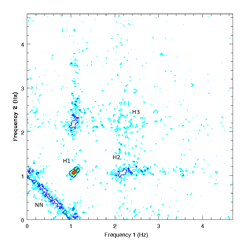
Figure 6: The bicoherence plot for observation 10408-01-25-00. The peak closest to H1 is the interaction between the fundamental and the second harmonic, the peak closest to H2 is the region for the interaction between the fundamental and the second harmonic to produce the third harmonic, and the weak peak closest to H3 is the interaction of the second harmonic with itself to produce the fourth harmonic. The diagonal stripe marked NN is the region where the two noise components add up to the frequency of the fundamental.

In this system we can examine the biphases of the few strongest peaks in the bispectrum to get a feel for the properties of the strongest set of waves in the system. The peak of our bicoherence is $f_{1}=36,f_{2}=37$ with the units of the frequency here being the frequency resolution of the power spectrum, 0.03125 Hz (i.e. 1/32 Hz). The biphases for all combinations where $f_{1}$ and $f_{2}$ both range from 35 to 38 times the frequency resolution are found in the range from 0.82$\pi$ to $0.97\pi$, with the mean being $0.86\pi$ and the standard devation on the phase, estimated from the variance in the measured values, is $0.05\pi$ – this can be seen in the bicoherence plot as the region marked H1 in figure 6. For the case where the first and second harmonics interact to produce the third harmonic, with $f_{1}$ from bins 35 to 38 and $f_{2}$ form bins 71 to 75, then mean value of the biphase is $0.22\pi$ with a standard deviation of $0.08\pi$ and a standard deviation of the mean of $0.02\pi$ – this can be seen as region H2 in figure 6. For the case where the second harmonic interacts with itself to produce the fourth harmonic, (i.e where $f_{1}$ and $f_{2}$ range from 71 to 75 times the frequency resolution of the power spectrum), we find that the mean biphase is $0.11\pi$, with a standard deviation of $0.17\pi$ and a standard deviation of the mean of $0.04\pi$ – this can be seen as region H3 in figure 6, and it is clear from this figure that the bicoherence is quite weak at this peak. Because the fundamental and the second harmonic are stronger than the third and fourth harmonics, and the bicoherence is also stronger for the first two frequencies, the effects of the first two frequencies’ phase couplings have the major impact on the shape of the QPO in the light curve.

The biphase 0.86$\pi$ is quite close to $\pi$ itself. This means that the shape of the oscillation, as determined by just the two strongest frequencies is one marked by a relatively smooth profile apart from deep dips occurring on the fundamental frequency, with phase width of less than $\pi$. The folded light curve of the data, made using the efold tool within FTOOLS, shown in figure 7 looks as expected.

Figure 7: The light curve for observation 10408-01-25-00 folded on the period of the QPO of 0.849 seconds. One can clearly see the flux skewness in the time series.

We can also consider the case where the two noise frequencies add up to the fundamental QPO frequency, in the region marked NN in figure LABEL:bico. This, in fact, is the real power of the bispectrum, as this information cannot be obtained by folding the data on the QPO period. Here, we take call bispectrum measurements where $f_{1}+f_{2}$ ranges from 35 to 38 in units of the frequency resolution. We find all the values of the biphase to be between -0.12$\pi$ and 0.33$\pi$ with a mean value of the biphase of 0.14$\pi$, with a standard deviation of 0.09$\pi$ and a standard deviation of the mean of 0.01$\pi$. The value of this biphase is then a bit less than $\frac{1}{7}\pi$ – i.e. it is much closer to zero than to $\pi/2$, and the major property of the behavior of the source in terms of the interactions of the noise and the QPO should be that those expected for a “pulsar”-like system. That is, the “envelope” on which the QPO is imposed should be one of spikes shooting well above a baseline flux which is slightly below the mean. This is, in fact the case. When the light curve is binned on a timescale of $\frac{1}{16}$ second, the mean count rate is 8164 cts/sec, the minimum is 4160 counts/sec, and the maximum is 16272 counts/sec, roughly a factor of two above and below the mean. The skewness of the flux distribution is positive, as calculated using lcstats from within the FTOOLS. The system thus largely follows the expectation for a lognormal flux distribution, as is often observed for X-ray binaries’ light curves (Uttley et al. 2005). The deviation from a biphase of exactly zero suggests that on long timescales, the intensity of the QPO rises sharply and falls more slowly. While some power is present in the bicoherence above the QPO frequency, this power is weak, so we do not investigate the biphase there.

5.3 RXTE observation 20402-01-15-00: a medium frequency QPO with a “cross” pattern bicoherence: a nearly sawtooth pattern for the fundamental plus second harmonic

In observation 20402-01-15-00, the “cross” pattern is seen – the bicoherence is strong when the QPO has either the median or the lowest frequency of the three frequencies being considered, but the bicoherence is not above the noise level for the case where $f_{1}+f_{2}=f_{QPO}$, and $f_{1},f_{2}$ are two noise frequencies. We can now look at the biphases of the source. The QPO here peaks in frequency bin 72 (corresponding to a frequency of 2.2 Hz, given the 1/32 Hz frequency resolution), and shows a strong second harmonic.

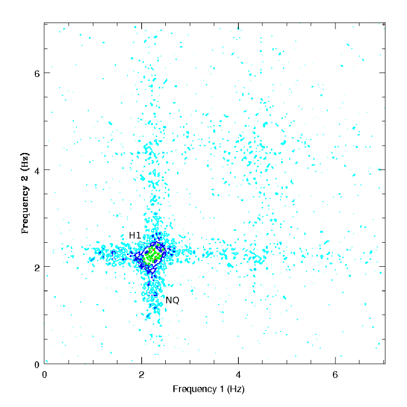
Figure 8: The bicoherence plot for observation 20402-01-15-00. The peak closest to H1 is the interaction between the fundamental and the second harmonic. The region just to the left of the NQ label is the region where the noise frequency plus the QPO frequency add up to the second noise frequency.

First let us examine the properties of the bispectrum for the frequencies in which the $f_{1}\approx{f_{2}}$ is the QPO frequency and $f_{1}+f_{2}$ is the frequency of the second harmonic of the QPO. We take the range of frequency bins from 69 to 76 in units of the frequency resolution – the region labelled H1 in figure 8. The biphases here range from $-0.16\pi$ to $-0.35\pi$, with a mean value of $-0.29\pi$, a standard deviation of 0.05$\pi$, and a standard deviation of the mean of 0.01$\pi$. As the biphase is $-0.29\pi$, the real component of the bispectrum is positive, indicating a flux distribution skewed to the bright end of the mean. The imaginary component is negative, indicating a fast rise, slow decay shape to the oscillation.

We can then look at the interactions between the QPO and the noise component, which are strong for the triplets of frequencies of $f_{1},f_{QPO}$ and $f_{1}+f_{QPO}$, where $f_{1}<f_{QPO}$ – the region labelled NQ in figure 8. In this case, the measurement errors are large on the biphases, and the values span nearly the full range of $2\pi$, so phase wrapping prevents us from using the mean and dispersion of the biphases values directly as has been done for the previous cases. In order to find a mean biphase, we average the sines of the biphases and the cosines of the biphases. We find that the final biphase has a value of $-0.21\pi$, and we take the variance in the mean value of the sines and cosines of the biphases and use standard error propagation to find a standard deviation of $0.09\pi$ and a standard deviation of the mean of $0.01\pi$. The shape of the light curve on these timescales is thus fairly similar to the shape of the QPO. As in the previous observation, while some power is present in the bicoherence above the QPO frequency, this power is weak, so we do not investigate the biphase there.

5.4 30184-01-01-000: hypotenuse pattern, high freq: a nearly sawtooth pattern for the fundamental plus second harmonic

In this observation, the bicoherence shows strong power on the timescale of the harmonic, and for the case where $f_{1}+f_{2}=f_{QPO}$, but not for any frequency higher than the fundamental frequency of the QPO, except at the harmonics of the QPO. For this observation, the QPO is at a frequency of approximately 3.4 Hz, peaking in bin 57 with a frequency resolution of 1/16 Hz. The bicoherence plot is given in figure 9.

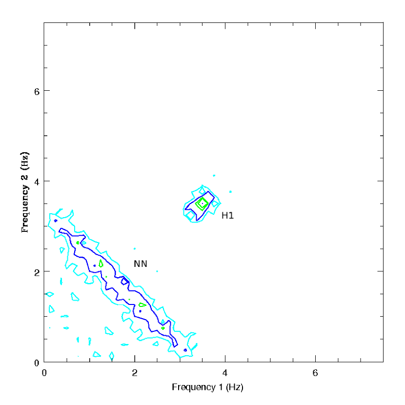
Figure 9: The bicoherence plot for observation 30184-01-01-000. The peak closest to H1 is the interaction between the fundamental and the second harmonic. The noise region examined is the diagonal near the label NN – as discussed in the text, because the QPO is extremely strong in this observations, the frequencies at the “ends” of the diagonals – i.e. those with one component relatively near 0 frequency and one relatively near the QPO frequency – are not included in the biphase computation.

First, we examine the coupling between the fundamental and the harmonic, the region marked H1 in figure 9. Taking all frequency bins from 55-59, we find that the biphasess all lie between $1.31\pi$ and $1.55\pi$, with a mean of 1.42 $\pi$, a standard deviation of $0.07\pi$, and a standard deviation of the mean of .01$\pi$. The flux distribution of the source here is thus nearly symmetric, while the time series itself has some asymmetry. The biphase for the interaction between the fundamental and the second harmonic indicates that the QPO rises quickly and decays slowly, as a decaying sawtooth wave. We note that the values of the squared bicoherence in this observation, even at the harmonic, are less than 0.05, indicating that the relative phases of the fundamental and the harmonic show substantial variation, and hence so does the shape of the oscillation – at the same time, the statistical significance of the difference between the bicoherence and zero is quite strong (M11), so the mean shape of the oscillation must be something like an inverse sawtooth wave.

The interaction of the QPO with the noise component shows a different behavior. Because the QPO is extremely strong in this observation, we must move far off the QPO centroid in order not to have the biphases estimates affected substantially by the wings of the QPO. We take the means of the sines and cosines of the biphases for all cases with $f_{1},f_{2}<45$ in units of the frequency resolution, and $f_{QPO}$ from 55 to 59 in the same units – this is the region marked NN is figure 9. We find that the mean biphase is $0.32\pi$ radians, with a standard deviation of $0.2\pi$ and a standard deviation of the mean of $0.02\pi$. The flux distribution is thus skewed to positive values. The time symmetry is that of a sawtooth wave with slow rise and fast decay – the QPO amplitude is rising slowly and turning off more quickly. Thus, when we compare with obseravation 10408-01-25-00, we see that in both observations, the interactions with the noise component are fairly similar, while the shapes of the oscillations themsleves are quite different.

6 Discussion

Since our previous paper, we have become aware of some mechanisms for producing some of the observed bicoherence patterns in a tidy manner. In particular, the “hypotenuse” pattern is reproduced very well by a bilinear oscillator (Rivola & White 1998; White 2009). The bilinear oscillator is a system described by a differential equation quite similar to that for a simple harmonic oscillator, except that the restoring force has a different normalization for positive and negative displacements. The bilinear oscillator is of interest to engineers because it provides a good mathematical description to a cracked or fatigued beam within a machine, and hence measuring the bispectrum of the machine in response to being driven by vibrations can allow the crack to be detected without taking apart the machine or waiting for the machine to suffer a catastrophic breakdown.

While obviously cracked beams do not exist in astrophysical situations, other types of force law with similar mathematical dependences may exist in accretion disks. If we find that the power spectrum and the bispectrum of the bilinear oscillator can give a good mathematical description of the time series we observe, then we can focus theoretical efforts on producing physical models that are mathematically similar to the bilinear oscillator.

Following White (2009), we calculate a bilinear oscillator which follows the equation:

$$\frac{d^{2}y}{dt^{2}}+c\frac{dy}{dt}+\kappa(y)y=x(t)$$ (4)

For a first run, we set $\kappa$ equal to 200000 for $y<0$ and to 1000000 for $y>0$. We set $c$ equal to 50, and we integrate over discretized time steps of .0003 time units, with an initial value of $y$ of 200. We drive the oscillator with a white noise process. The driving force has a mean expectation value of 0.0 and an expected standard deviation of $5.52\times 10^{6}$.

This run produces a bicoherence plot that looks quite similar to the hypotenuse pattern seen in the real data for observation 30184-01-01-000. The biphase for the QPO’s interaction with the harmonic here is very nearly 0. That is, the flux distribution is skewed to positive values, but the time series is symmetric in time. The same is true for the interactions of two noise components that add up to the QPO frequency. We next perform a simulation which is identical to the first, except that we exchange the values of $\kappa$ with respect to $y=0$ – i.e. we set $\kappa$ equal to 200000 for $y>0$ and to 1000000 for $y<0$. While the details of the time series are different the key statistical properties measured by the biphase are the same. We conduct a few experiments with stronger damping. Making the system more strongly damped decreases the bicoherence and broadens the QPO, but does not change the biphase substantially.

It thus appears that models mathematically similar to the bilinear oscillator are unlikely to produce the observed bispectra of X-ray binary light curves. There remains a catch, of course – the inherently oscillating parameter in a quasi-periodic oscillation is almost certainly not just the count rate. Models for the few Hz QPOs we discuss in this paper include models in which the disk undergoes a global oscillation due to the Lense-Thirring precession (e.g. Stella & Vietri 1998; Fragile et al. 2007), and thermal-viscous oscillations (Abramowicz et al. 1989; Chen & Taam 1994). In the Lense-Thirring pression model, the parameter oscillating is the inclination angle of the inner accretion disk, and the X-ray count rate will be a function of that inclination angle and may be modulated additionally, for example, by fluctations in the accretion rate changing the surface brightness of the disk in ways independent (or, at least, not directly tied to) of the observer’s inclination angle (some initial exploration of this possibility has been made in Ingram & Done 2011). Numerical calculations made to date do not cover enough cycles of the oscillation to allow calculations of the biphase of oscillations from the Lense-Thirring precession, but it is intriguing that the one published numerical calculation which includes ray tracing does seem to show qualitatively similar phenomenology to that see in observation 30184-01-01-000 (Dexter & Fragile 2011). It would also be straightforward for the Lense-Thirring model to produce periodic occultations of part of the accretion disk, and hence to produce a biphase of approximately $\pi$ – this has been considered in Ingram & Done (2012), although the bispectrum of the simulation has not yet been computed. In principle, the same type of ray tracing calculations used in Dexter & Fragile (2011) could be run over a wider range of parameter space to detemine whether the biphase properties could be matched in a manner that is also consistent with the additional information given from other system parameters such as the mass accretion rate. In some cases, also, higher order corrugation modes may be present (see e.g. Tsang & Lai 2009).

The situation for the thermal viscous oscillation is perhaps even more difficult to reconcile with the data. The simulated light curves of Chen & Taam (1994) show slow rises, followed by quick decays of the flux. This would be expected to produce a biphase near $\pi/2$, giving opposite behavior to that seen, for example, observation 30184-01-01-000. Other models exist for explaining the low frequency quasi-periodic oscillations in X-ray binaries, and have the accompanied by noise components, but at present, simulated light curves for them have not been presented which could allow us to determine under what conditions the observed biphases might be reproduced (e.g. Varniére & Tagger 2002; Machida & Matsumoto 2008).

In future work, the biphase analysis may also be extended to help develop a better understanding of the light curves of sources without strong quasi-periodic oscillations. In particular, the recent development of an analytic method for calculating simulated light curves from propagation models (Ingram & van der Klis 2013) should allow one to study these models efficiently to determine how well they match the observed data in biphase. Given that the flux distributions of X-ray binaries are widely found to be log-normal when they are dominated by noise components (Uttley et al. 2005), we can reasonably expect that in all cases, the real component of the biphase will be positive. We can also expect that the imaginary components will be positive as well, given that the fastest variability is expected at the highest count rates due to the higher rate of energy generation in the inner part of the accretion flow. The exact value of the biphase is likely to trace the emissivity of the accretion flow.

7 Summary

We have presented an introduction to the use of the biphase aimed at astronomers wishing to apply it to time series analysis. First, we briefly summarize the meaning of the biphase, so that a quick look at its value can be used to develop a quick intuition about the properties of a timeseries.

1. Time series which are symmetric in time have purely real bispectra, and time series which have flux distributions symmetric about the mean have purely imaginary bispectra.

2. When the real component is positive, the flux distribution is skewed to positive values.

3. Thus spiky time series like pulsar light curves will have biphases near 0.

4. Time series like eclipsing binary light curves will have biphases near $\pi$.

5. When the imaginary component is positive, the time series rises slowly and fades quickly. This yields biphases near $\pi/2$.

6. When the imaginary component is negative, the time series rises quickly and fades slowly. This yield biphases near $-\pi/2$.

We have also applied the biphase to several obseravtions of GRS 1915+105. We have found that the profile of the QPO matches well between light curves produced by folding on the QPO period and the predictions from the biphase data. We have also found that the actual values of the biphases vary widely from observation to observation. No simple models that we have considered can reproduce the observed biphase data.

8 Acknowledgments

I am grateful to Michiel van der Klis, Chris Fragile, Patricia Arévalo, Simon Vaughan, and to Paul White of the University of Southampton’s Institute for Sound and Vibration Research for extremely interesting and valuable discussions. I also thank the Astrophysis Insitute of the Canary Islands for hospitality while a portion of this work was completed. Finally, I thank the referee, Adam Ingram, for a report which was both prompt and helpful, and which has led to improvements in the clarity and content of the paper.

References

- [1] Aigrain S., Favata F., Gilmore G., 2004, A&A, 414, 1139
- [2] Abramenko V.I., 2005, ApJ, 629, 1141
- [3] Abramowicz M.A., Szuszkiewicz E., Wallinder F., 1989, in Theory of Accretion Disks, eds. F. Meyer, W.J. Duschl, J. Frank, E.Meyer-Hofmeister (Dordrecht: Kluwer), 141
- [4] Davies R.B., Harte D.S., 1987, Biometrika, 74, 95
- [5] Dexter J., Fragile P.C., 2011, ApJ, 730, 36
- [6] Edelson R.A., Krolik J.H., 1988, ApJ, 333, 646
- [7] Elgar S., Guza R.T., 1985, J. Fluid Mech., 161, 425
- [8] Fackrell J., 1997, PhD Thesis, University of Edinburgh
- [9] Feroci M., et al., 2012, Experimental Astronomy, 34, 415
- [10] Gajraj R.J., Doi M., Matzaridis H., Kenny G.N., 1998, British Journal of Anaesthesia, 80, 46
- [11] Gaskell C.M., 2004, ApJ, 612, L21
- [12] Hasselman K.W., Munk W. & MacDonald G., 1963, Time Series Analysis, John Wiley: New York, M. Rosenblatt editor, p.125
- [13] Haug E.G., Taleb N.N., 2011, Journal of Economic Behavor and Organization, 77
- [14] Hesse K.H., Wielebinski R., 1974, A&A, 31, 409
- [15] Ingram A., Done C., 2011, MNRAS, 415, 2323
- [16] Ingram A., Done C., 2012, MNRAS, 419, 2369
- [17] Jiang C., et al., 2011, ApJ, 742, 120
- [18] Kamionkowski M., Smith T.L., Heavens A., 2011, PhysRevD, 83, 023007
- [19] Klassen A., Aurass H., Mann G., 2001, A&A, 370, L41
- [20] Loeb A., Gaudi B.S., 2003, ApJ, 588L, 117
- [21] Lyutyj V.M. & Oknyanskij V.L., 1987, AZh, 64, 465
- [22] Maccarone T.J., Coppi P.S., 2002, MNRAS, 336, 817
- [23] Maccarone T.J., Coppi P.S., Poutanen J., 2000, ApJ, 537L, 107
- [24] Maccarone T.J., Uttley P., van der Klis M., Wijnands R.A.D., Coppi P.S., 2011, MNRAS, 413, 1819 (M11)
- [25] Machida M., Matsumoto R., 2008, PASJ, 60, 613
- [26] Makuch R.W., Freeman D.H., Johnson M.F., 1979, Journal of Chronic Disease, 32, 245
- [27] Masada A., Kuo Y.-Y., 1981, Deep Sea Research, 28A, 213
- [28] McComas C.H., Briscoe M.G., 1980, Journal of Fluid Mechanics, 97, 205
- [29] Nowak M.A., Vaughan B.A., Wilms J., Dove J.B., Begelman M.C., 1999, ApJ, 510, 874
- [30] Priedhorsky W., Garmire G.P., Rothschild R., Boldt E., Serlemitsos P., Holt S., 1979, ApJ, 233, 350
- [31] Rivola A., White P., 1998, Journal of Sound and Vibration Research, 216, 889
- [32] Scaringi S., Körding, E., Uttley, P., Knigge, C., Groot, P. J., Still, M., 2012, MNRAS, 421, 2854
- [33] Shaposhnikov N., 2012, astro-ph/1205.0748
- [34] Terrell N.J., 1972, ApJ, 174L, 35
- [35] Timmer J., Koenig M., 1995, A&A, 300, 707
- [36] Uttley P., McHardy I.M., 2001, MNRAS, 323L, 26
- [37] Uttley P., McHardy I.M., Vaughan S., 2005, MNRAS, 359, 345
- [38] van Milligen B.P., Sanchez E., Estrada T., Hidalgo C., Branas B., Carreras B., Garcia L., 1995, Physics of Plasmas, 2, 3017
- [39] Varnière P., Tagger M., 2002, A&A, 394, 329
- [40] Way M.J., Scargle J.D., Ali K.M., Srivastava A.N., 2012, “Advances in Machine Learning and Data Mining for Astronomy”, CRC Press: Boca Raton
- [41] White P.R., 2009, in Encyclopedia of Structural Health Monitoring, editors C.Boller, F.-K. Chang and Y. Fujino, Wiley:Hoboken
- [42] Zweibel E. G., Yamada M., 2009, ARA&A, 47, 291