Dust in the diffuse interstellar medium

We present a model for the diffuse interstellar dust that explains the observed wavelength-dependence of extinction, emission, linear and circular polarisation of light. The model is set-up with a small number of parameters. It consists of a mixture of amorphous carbon and silicate grains with sizes from the molecular domain of 0.5 up to about 500 nm. Dust grains with radii larger than 6 nm are spheroids. Spheroidal dust particles have a factor 1.5 – 3 larger absorption cross section in the far IR than spherical grains of the same volume. Mass estimates derived from submillimeter observations that ignore this effect are overestimated by the same amount. In the presence of a magnetic field, spheroids may be partly aligned and polarise light. We find that polarisation spectra help to determine the upper particle radius of the otherwise rather unconstrained dust size distribution. Stochastically heated small grains of graphite, silicates and polycyclic aromatic hydrocarbons (PAHs) are included. We tabulate parameters for PAH emission bands in various environments. They show a trend with the hardness of the radiation field that can be explained by the ionisation state or hydrogenation coverage of the molecules. For each dust component its relative weight is specified, so that absolute element abundances are not direct input parameters. The model is confronted with the average properties of the Milky Way, which seems to represent dust in the solar neighbourhood. It is then applied to specific sight lines towards four particular stars one of them is located in the reflection nebula NGC 2023. For these sight lines, we present ultra-high signal-to-noise linear and circular spectro-polarimetric observations obtained with FORS at the VLT. Using prolate rather than oblate grains gives a better fit to observed spectra; the axial ratio of the spheroids is typically two and aligned silicates are the dominant contributor to the polarisation.

1 Introduction

Interstellar dust grains absorb, scatter, and polarise radiation and emit the absorbed radiation through non-thermal and thermal mechanisms. Dust grains not only absorb and scatter stellar photons, but also the radiation from dust and gas. In addition, interstellar dust in the diffuse interstellar medium (ISM) and in other environments that are illuminated by UV photons show photoluminescence in the red part of the spectrum, a contribution known as Extended Red Emission (ERE, Cohen et al. 1975; Witt et al. 1984).

Clues to the composition of interstellar dust come from observed elemental depletions in the gas phase. It is generally assumed, that the abundances of the chemical elements in the ISM are similar to those measured in the photosphere of the Sun. The abundances of the elements of the interstellar dust (the condensed phase of matter) are estimated as the difference between the elemental abundances in the solar photosphere (Asplund et al. 2009) and that of the gas-phase. Absolute values of the interstellar gas-phase abundance of element [X] are given with respect to that of hydrogen [H]. Such [X]/[H] ratios are often derived from the analysis of absorption lines. (Note that oscillator strengths of some species e.g., CII 2325Å are uncertain up to a factor of 2, see discussion in Draine 2011). The most abundant condensible elements in the ISM are C, O, Mg, Si and Fe. When compared to the values of the Sun, elements such as Mg, Si and Fe, which form silicates, in the gas-phase appear under–abundant. By contrast, oxygen represents a striking exception, as it appears over–abundant towards certain sight-lines (Voshchinnikov & Henning 2010). Another important dust forming element, C, cannot be characterised in detail because it has been analysed only in a restricted number of sight-lines, leading in some cases to inaccurate values of its abundance (Jenkins 2009); Parvahti et al. 2012). It is widely accepted that cosmic dust consists of some form of silicate and carbon.

Stronger constraints on the composition of interstellar grains come from the analysis of their spectroscopic absorption and emission signatures. The observed extinction curves display various spectral bands. The most prominent ones are the 2175 Å bump, where graphite and polycyclic aromatic hydrocarbons (PAHs) have strong electronic transitions, and the 9.7 $\mu$m and 18 $\mu$m features assigned to Si-O stretching and O-Si-O bending modes of silicate minerals, respectively. In addition, there are numerous weaker features, such as the 3.4 $\mu$m absorption assigned to C-H stretching modes (Mennella et al. 2003), and the diffuse interstellar bands in the optical (Krelowski 2002). The observed 9.7 and 18 $\mu$m band profiles can be better reproduced in the laboratory by amorphous silicates than crystalline structures. Features that are assigned to crystalline silicates, such as olivine (Mg_2x Fe_2-2x SiO₄ with $x\sim 0.8$), have been detected in AGB and T Tauri stars and in comet Hale-Bopp (see Henning 2010 for a review). However, since these features are not seen in the ISM, the fraction of crystalline silicates in the ISM is estimated $\la 2$ % (Min et al. 2007). Dust in the diffuse ISM appears free of ices that are detected in regions shielded by $A_{\rm V}>1.6$ mag (Bouwman et al. 2011, Pontoppidan et al. 2003, Siebenmorgen & Gredel 1997, Whittet et al. 1988).

In the IR, there are conspicuous emission bands at 3.3, 6.2, 7.7, 8.6, 11.3 and 12.7 $\mu$m, as well as a wealth of weaker bands in the 12 – 18 $\mu$m region. These bands are ascribed to vibrational transitions in PAH molecules. PAHs are planar structures, and consist of benzol rings with hydrogen attached. Less perfect structures may be present where H atoms are replaced by OH or CN and some of the C atoms by N atoms (Hudgins et al. 2005). PAHs may be ionised: PAH⁺ cations may be created by stellar photons, and PAH^- anions may be created by collisions of neutral PAHs with free e^-. The ionisation degree of PAH has little influence on the central wavelength of the emission bands, but has a large impact on the feature strengths (Allamandola et al. 1999, Galliano et al. 2008). Feature strengths also depend on the hardness of the exciting radiation field, or on the hydrogenation coverage of the molecules (Siebenmorgen & Heymann 2012).

The extinction curve gives the dust extinction as a function of wavelength. It provides important constraints on dust models, and in particular on the size distribution of the grains. Important work has been published by Mathis et al. (1977), who introduced their so–called MRN size distribution, and by Greenberg (1978), who have presented his grain core–mantle model. Another important constraint on dust models is provided by the IR emission. IRAS data revealed stronger than expected 12 and 25 $\mu$m emission from interstellar clouds (Boulanger et al. 1985). At the same time, various PAH emission bands have been detected (Allamandola et al. 1985, 1989, Puget & Léger 1989). Both emission components can only be explained by considering dust particles that are small enough to be stochastically heated. A step forward was taken in the dust models by Désert et al. (1990), Siebenmorgen & Krügel (1992), Dwek et al. (1997), Li & Draine (2001), and Draine & Li (2007). In these models, very small grains and PAHs are treated as an essential grain component beside the (so far) standard carbon and silicate mixture of large grains.

In all these studies, large grains are assumed to be spherical and, the particle shape is generally not further discussed. However, in order to account for the widely observed interstellar polarisation, non–spherical dust particles partially aligned by some mechanism need to be considered. This has been done e.g. by Hong & Greenberg (1980), Voshchinnikov (1989), Li & Greenberg (1997) who considered infinite cylinders. More realistic particle shapes such as spheroids have been considered recently. The derivation of cross sections of spheroids is an elaborate task, and computer codes have been made available by Mishchenko (2000) and Voshchinnikov & Farafonov (1993). The influence of the type of spheroidal grain on the polarisation is discussed by Voshchinnikov (2004). Dust models considering spheroidal particles that fit the average Galactic extinction and polarization curves were presented by Gupta et al. (2005), Draine & Allaf-Akbari (2006), Draine & Fraisse (2009). The observed interstellar extinction and polarization curves towards particular sight lines are modelled by Voshchinnikov & Das (2008) and Das et al. (2010).

In this paper we present a dust model for the diffuse ISM that accounts for observations of elemental abundances, extinction, emission, and interstellar polarisation by grains. The ERE is not polarised and is not further studied in this work (see Witt & Vijh 2004 for a review). We also do not discuss diffuse interstellar bands as their origin remains unclear (Snow & Destree, 2011) nor various dust absorption features observed in denser regions. We first describe the light scattering and alignment of homogeneous spheroidal dust particles and discuss the absorption properties of PAHs. Then we present our dust model. It is first applied to the observed average extinction and polarisation data of the ISM, and the dust emission at high Galactic latitudes. We present dust models towards four stars for which extinction and IR data are available, and for which we have obtained new spectro–polarimetric observations with the FORS instrument of the VLT. We conclude with a summary of the main findings of this work.

2 Model of the interstellar dust

2.1 Basic definitions

Light scattering by dust is a process in which an incident electromagnetic field is scattered into a new direction after interaction with a dust particle. The directions of the propagation of the incident wave and the scattered wave define the so–called scattering plane. In this paper we define the Stokes parameters I, Q, U, V as in Shurcliff (1962), adopting as a reference direction the one perpendicular to the scattering plane. This way, the reduced Stokes parameter $P_{Q}=Q/I$ is given by the difference between the flux perpendicular to the scattering plane, $F^{\bot}$, minus the flux parallel to that plane, $F^{\|}$, divided by the sum of the two fluxes. In the context of this paper, Stokes $U$ is always identically zero, so that $P_{Q}$ is also the total fraction of linear polarisation $p$.

We now define $\tau^{\|}$ and $\tau^{\bot}$ as the extinction coefficients in the two directions, and $\tau_{\rm eff}=(\tau^{\|}+\tau^{\bot})/2$. In case of weak extinction ($\tau_{\rm eff}\ll 1$), and since $|\tau^{\|}-\tau^{\bot}|\ll 1$, the polarisation by dichroic absorption is approximated by

$$p={{F^{\bot}-F^{\|}}\over{F^{\bot}+F^{\|}}}={{e^{\tau^{\|}}-e^{\tau^{\bot}}}\over{e^{\tau^{\bot}}+e^{\tau^{\|}}}}\simeq\frac{\tau^{\|}-\tau^{\bot}}{2}\,.$$ (1)

A medium is birefringent if its refractive index depends on the direction of the wave propagation. In this case, the phase velocity of the radiation also depends on the wave direction, and the medium introduces a phase retardation between two perpendicular components of the radiation, transforming linear into circular polarisation. In the ISM, a first scattering event in cloud 1 will linearly polarise the incoming (unpolarised) radiation, and a second scattering event in cloud 2 will transform part of this linear polarisation into circular polarisation. Denoting by $p(1)$ the fraction of linear polarised induced during the first scattering event, and by $N_{d}(2)$ the dust column density in cloud 2, and with $\Psi$ the difference of positional angles of polarisation in clouds 1 and 2, the circular polarisation $p_{\rm c}$ is a second order effect and given by

$$p_{\rm c}=\frac{V}{I}=N_{d}(2)C_{c}(2)\ \times\ p(1)\sin(2\Psi)\,,$$ (2)

where $C_{c}$ is the cross section of circular polarisation (birefringence) calculated as the difference in phase lags introduced by cloud 2. Light propagation in a medium in which the grain alignment changes is discussed by Martin (1974) and Clarke (2010). The wavelength dependence and degree of circular polarisation is discussed by Krügel (2003) and that of single light scattering by asymmetric particles by Guirado et al. (2007).

2.2 Spheroidal grain shape

The phenomenon of interstellar polarisation cannot be explained by spherical dust particles consisting of optically isotropic materials. Therefore, as a simple representation of finite sized grains, we consider spheroids. The shape of spheroids is characterised by the ratio $a/b$ between major and minor semi-axes. There are two types of spheroids: prolates, such as needles, which are mathematically described by rotation about the major axis of an ellipse, and oblates, such as pancakes, obtained from the rotation of an ellipse about its minor axis. In our notation, the volume of a prolate is the same of a sphere with radius $r=(a\cdot b^{2})^{1/3}$, and the volume of an oblate is that of a sphere with radius $r=(a^{2}\cdot b)^{1/3}$.

The extinction optical thickness, which is due to absorption plus scattering by grains of radius $r$, is given by

$$\tau({\nu})=N_{\rm d}\ C_{\rm ext}({\nu})$$ (3)

and similar the linear polarisation by

$$p(\nu)=N_{\rm d}\ C_{\rm p}({\nu})\,,$$ (4)

where $N_{\rm d}$ is the total column density of the dust grains along the line of sight and $C_{\rm{ext,p}}$ are the extinction and linear polarisation cross sections.

2.3 Dust alignment

Stellar radiation may be polarised by partially aligned spheroidal dust grains that wobble and rotate about the axis of greatest moment of inertia. The question on how grain alignment works is not settled. Various mechanisms such as magnetic or radiation alignment are suggested, see Voshchinnikov (2012) for a review. We consider grain alignment along the magnetic field $\@vec{B}$ that is induced by paramagnetic relaxation of particles having Fe impurities. This so–called imperfect Davis-Greenstein (IDG) orientation of spheroids can be described by

Figure 1: Geometrical configuration of a spinning and wobbling prolate spheroidal grain with notation by Das et al. (2010). The major axis O₁O₂ of the particle spheroid is placed in the spinning plane NO₁O₂ that is perpendicular to the angular momentum $\@vec{J}$. Direction of the light propagation $\@vec{k}$ is set parallel to the $Z$-axis. We measure from $Z$ the angle $0\leq\Omega\leq 90\degr$ to the magnetic field $\@vec{B}$, the angle $\alpha$ to the major rotation axis of the particle and the angle $\theta$ to the angular momentum $\@vec{J}$; $\varphi$ is the spin angle, $\beta$ is the precession-cone angle, and $\omega$ the current precession angle.

$${f}(\xi,\beta)=\frac{\xi\sin\beta}{(\xi^{2}\cos^{2}\beta+\sin^{2}\beta)^{3/2}}\,,$$ (5)

where $\beta$ is the precession-cone angle defined in Fig. 1, and

$$\xi^{2}=\frac{r+\delta_{0}\ (T_{\rm d}/T_{\rm g})}{r+\delta_{0}}\,.$$ (6)

The alignment parameter, $\xi$, depends on the size of the particle, $r$. The parameter $\delta_{0}$ is related to the magnetic susceptibility of the grain, its angular velocity and temperature, the field strength and gas temperature (Hong & Greenberg 1980). Voshchinnikov & Das (2008) show that the maximum value of the polarisation depends on $\delta_{0}$, whereas the spectral shape of the polarisation does not. Das et al. (2010) are able to fit polarisation data by varying the size distribution of the dust particles and by assuming different alignment functions. We simplify matters and choose $\delta_{0}=10\mu$m and $T_{\rm g}=10\ T_{\rm d}$. If the grains are not aligned ($\xi=1$) then ${f}(\xi,\beta)=\sin\beta$; in the case of perfect rotational alignment $\xi=0$. In the IDG mechanism (Eq. 6) smaller grains are better aligned than larger ones.

2.4 Cross sections of spheroids

Cross sections of spinning spheroids change periodically. We compute the average cross section of spinning particles following Das et al. (2010). Such mean extinction ${C}_{\rm ext}$, linear ${C}_{\rm p}$ and circular polarisation ${C}_{{\rm c}}$ cross sections of a single-sized homogeneous spheroidal particle are obtained at a given frequency $\nu$ by:

$${C}_{{\rm ext}}(\nu)=\frac{2}{\pi}\int(Q_{{\rm ext}}^{\rm{TM}}+Q_{{\rm ext}}^{\rm{TE}})\,r^{2}\,f(\xi,\beta)\,\mathrm{d}{\varphi}\,\mathrm{d}{\omega}\,\mathrm{d}{\beta}\,,$$ (7)

$${C}_{{\rm p}}(\nu)=\frac{1}{\pi}\int(Q_{{\rm ext}}^{\rm{TM}}-Q_{{\rm ext}}^{\rm{TE}})\,r^{2}\,f(\xi,\beta)\,\cos(2{\psi})\,\mathrm{d}{\varphi}\,\mathrm{d}{\omega}\,\mathrm{d}{\beta}\,,$$ (8)

$${C}_{{\rm c}}(\nu)=\frac{1}{\pi}\int(Q_{{\rm pha}}^{\rm{TM}}-Q_{{\rm pha}}^{\rm{TE}})r^{2}f(\xi,\beta)\cos(2{\psi})\,\mathrm{d}{\varphi}\,\mathrm{d}{\omega}\,\mathrm{d}{\beta}\,.$$ (9)

Angles $\psi,\,\varphi,\,\omega,\,\beta$ are shown in Fig. 1. The relations between them are defined by Hong & Greenberg (1980). The efficiency factors $Q$ in Eqs. (7 – 9), with suffix TM for the transverse magnetic and TE for transverse electric modes of polarisation (Bohren & Huffman 1983), are defined as the ratios of the cross sections to the geometrical cross-section of the equal volume spheres, $Q=C/\pi r^{2}$. The extinction and scattering efficiencies $Q_{{\rm ext}}$, $Q_{{\rm sca}}$ and phase lags $Q_{{\rm pha}}$ of the two polarisation directions are computed with the program code provided by Voshchinnikov & Farafonov (1993). The average absorption and scattering cross sections ${C}_{{\rm abs,sca}}$ are obtained similar to Eq. (7) utilizing $Q_{{\rm abs,sca}}$, respectively.

Table 1: Band parameters of astronomical PAHs.

Center Wavelength		Damping Constant			Integrated Cross Sectiona			Modeb
$\lambda_{0}$ ($\mu$m)		$\gamma$ ($10^{12}$s-1)			$\sigma_{\rm int}$ ($10^{-22}$cm2$\mu$m)
ISM +	NGC 2023	Starburstsc	ISMd	NGC 2023d	Starburstsc	ISMd	NGC 2023d
Starbursts
0.2175		$\cdots$	1800	1800	$\cdots$	8000	8000	$\pi^{*}\leftarrow\pi$ transitions
3.3	$\cdots$	20	20	20	10	20	20	C-H stretch
5.1	$\cdots$	12	20	20	1	2.7	2.7	C-C vibration
6.2	$\cdots$	14	14	14	21	10	30	C-C vibration
7.0	$\cdots$	6	6	5	13	5	10	C-H?
7.7	$\cdots$	22	22	20	55	35	55	C-C vibration
8.6	$\cdots$	6	6	10	35	20	35	C-H in-plane bend
11.3	$\cdots$	4	6	4	36	250	52	C-H solo out-of-plane bend
11.9	$\cdots$	7	7	7	12	60	12	C-H duo out-of-plane bend
12.7	$\cdots$	3.5	5	3.5	28	150	28	C-H trio out-of-plane bend
13.6	$\cdots$	4	4	4	3.7	3.7	3.7	C-H quarto out-of-plane
14.3	$\cdots$	5	5	5	0.9	0.9	0.9	C-C skeleton vibration
15.1	15.4	3	4	4	0.3	0.3	0.3	C-C skeleton vibration
15.7	15.8	2	5	4	0.3	0.3	5	C-C skeleton vibration
16.5	16.4	3	10	1	0.5	5	6	C-C skeleton vibration
18.2	17.4	3	10	0.2	1	3	1	C-C skeleton vibration
21.1	18.9	3	10	0.2	2	2	2	C-C skeleton vibration
23.1	$\cdots$	3	10	4	2	2	1	C-C skeleton vibration

Notes.^aCross sections are integrated over the band and are given per H atom for C-H vibrations, and per C atom for C-C modes; ^bAssignment following Tielens (2008), Moutou et al. (1996), Pauzat et al. (1997); ^c Siebenmorgen et al. (2001); ^d this work (Sect. 4.1, Sect. 5).

2.5 Cross sections of PAHs

Strong infrared emission bands in the 3 – 13 $\mu$m range are observed in a variety of objects. The observations can be explained by postulating as band carriers UV-pumped large PAH molecules that show IR fluorescence. PAHs are an ubiquitous and important component of the ISM. A recent summary of the vast literature of astronomical PAHs is given by Joblin & Tielens (2011).

Unfortunately, the absorption cross section of PAHs, $C_{\rm{PAH}}$, remains uncertain. PAH cross sections vary by large factors from one molecule species to the next and they depend strongly on their hydrogenation coverage and charge state. Still in $C_{\rm{PAH}}$ one notices a spectral trend: molecules have a cut-off at low (optical) frequencies that depends on the PAH ionisation degree (Schutte et al. 1993, Salama et al. 1996), a local maximum near the 2175 Å  extinction bump (Verstraete & Léger 1992; Mulas et al. 2011), and a steep rise in the far UV (Malloci et al. 2011; Zonca et al. 2011).

We guide our estimates of the absorption cross section at photon energies between 1.7–15 eV of a mixture of ionised and neutral PAH species to the theoretical studies by Malloci et al. (2007). We follow Salama et al. (1996) for the cut-off frequency $\nu_{\rm{cut}}$ or cut-off wavelength: $\lambda_{\rm{cut}}^{-1}\ =\ 1+3.8\times({0.4\,N_{\rm C}})^{-0.5}$ ($\mu$m)^-1 and set $\lambda_{\rm{cut}}\geq 0.55\mu$m. The cross section towards the near IR is given by Mattioda et al. (2008, their Eq. 1):

$$C_{\rm M}(\nu)=N_{\rm C}\ \kappa_{\rm{UV}}\ {10^{-1.45\lambda}}\quad{\rm{:}}\quad\nu\leq\nu_{\rm{cut}}\,,$$ (10)

where $N_{\rm{C}}$ is the number of carbon atoms of the PAHs, $\kappa_{\rm{UV}}=1.76\times 10^{-19}$  (cm²/C-atom); energetically unimportant features near 1$\mu$m are excluded. The 2175 Å bump is approximated by a Lorentzian profile (Eq.11). In the far UV at $\lambda^{-1}>6\mu$m^-1, the cross section is assumed to follow that of similar sized graphite grains. The influence of hard radiation components on PAHs is discussed by Siebenmorgen & Krügel (2010). The size of a PAH, which are generally non-spherical molecules, can be estimated following Tielens (2005), by considering the radius of a disk of a centrally condensed compact PAH that is given by $r\sim 0.9{N_{\rm C}}^{0.5}$ (Å).

With the advent of ISO and Spitzer more PAH emission features and more details of their band structures have been detected (Tielens 2008). We consider 17 emission bands and apply, for simplicity, a damped oscillator model. Anharmonic band shapes are not considered despite having been observed (Peeters, et al. 2002, van Diedenhoven et al. 2004). The Lorentzian profiles are given by

$$C_{\rm L}(\nu)\ =\ N_{\rm{C,H}}\cdot\sigma_{\rm int}\;{\nu_{0}^{2}\over c}\cdot{\gamma\nu^{2}\over\pi^{2}(\nu^{2}-\nu_{0}^{2})^{2}+(\gamma\nu/2)^{2}}\,,$$ (11)

where $N_{\rm{C,H}}$ is the number of carbon or hydrogen atoms of the PAHs in the particular vibrational mode at the central frequency $\nu_{0}=c/\lambda_{0}$ of the band, $\sigma_{\rm{int}}=\int{\sigma_{\lambda}\mathrm{d}\lambda}$ is the cross section of the band integrated over wavelength, and $\gamma$ is the damping constant. PAH parameters are calibrated by Siebenmorgen & Krügel (2007) using mid-IR spectra of starburst nuclei and are listed in Table 1. Their procedure first solved the radiative transfer of a dust embedded stellar cluster, which contains young and old stellar populations. A fraction of the OB stars are in compact clouds that determine the mid IR emission. In a second step, the model is applied to NGC 1808, a particular starburst, and the mid-IR cross-sections of PAHs are varied, until a satisfactory fit to the ISO spectrum is found (Siebenmorgen et al. 2001). Finally, the so derived PAH cross-sections are validated by matching the SED of several well studied galaxies. In this latter step, the PAH cross-sections are held constant and the luminosity, size and obscuration of the star cluster is varied (Siebenmorgen et al. 2007). Efstathiou & Siebenmorgen (2009) and other colleagues, using the starburst library, have further confirmed the applied PAH mid–IR cross–sections. The total PAH cross section, $C_{\rm{PAH}}$, is given as the sum of the Lorentzians (Eq. 11) and the continuum absorption (Eq. 10).

In Fig.2, we show the PAH absorption cross-sections suggested by Li & Draine (2001), Malloci et al. (2007), this work, as well as the cross-section of a particular PAH molecule, Coronene (Mulas priv.com.). In the far UV the PAH cross sections agree within a factor of two. Near the 2200 Å bump we apply for the absorption maximum the same frequency and strength as Li & Draine (2001) but a slightly smaller width. Our choice of the width is guided by Coronene, which has a feature shifted to 2066 Å. Malloci et al. (2007) derive a mean PAH absorption cross section by averaging over more than 50 individual PAHs, which are computed in four charge states of the molecules. Such a procedure may cause a slight overestimate of the width of the PAH band near the 2200 Å bump, because different molecules show a peak at different frequencies in that region (for an example, see Coronene in Fig.2). Between 3 and 4 $\mu$m^-1 the cross section by Malloci et al. (2007) and Li& Draine (2001) are identical and agree within a factor $\sim 3$ to that one derived for Coronene. In the lower panel of Fig.2 PAH absorption cross sections between $1-30\,\mu$m are displayed for Coronene, neutral PAH-graphite particles with 60 C atoms (Li & Draine, 2001), and fitting results of this work, one for the solar neighbourhood (labelled ISM) and a second for the reflection nebulae NGC 2023 (Table 1). In the near IR, below 3 $\mu$m, the PAH cross sections are orders of magnitude smaller than in the optical. The scatter in the near IR cross sections of PAH is energetically not important for computing the emission spectrum at longer wavelengths. In the emission bands we find similar cross sections as Li & Draine for neutral species whereas those for ionised PAHs are larger by a factor of 10. Our model differs to the one by Li & Draine as we explain most of the observed ratios of PAH emission bands by de-hydrogenation rather than by variations of the PAH charge state (see Fig.1 in Siebenmorgen & Heymann, 2012). Beyond 15$\mu$m a continuum term is often added to the PAH cross sections (Désert et al. 1990; Schutte et al. 1993; Li & Draine 2001; Siebenmorgen et al. 2001). We neglect such a component as it requires an additional parameter and is not important for this work.

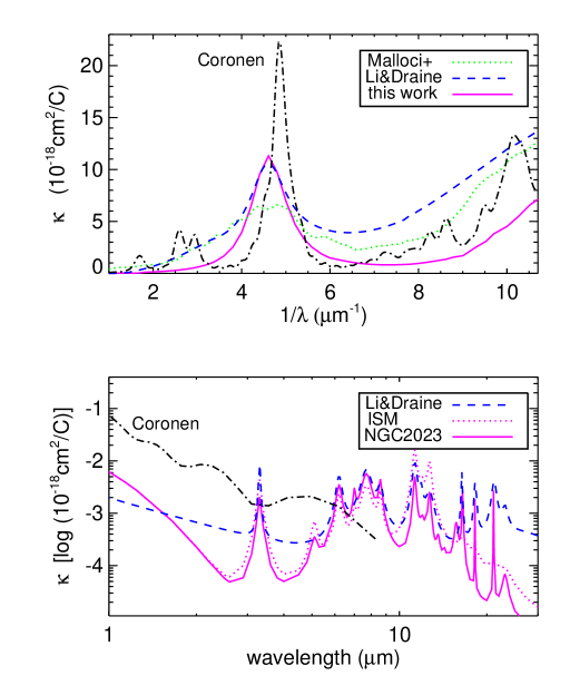
Figure 2: Absorption cross-sections of PAHs in the optical/UV (top) and infrared (bottom) as suggested by Li & Draine (2001, dashed blue), Malloci et al. (2007, dotted green) and this work, with parameters of Table 1 for the ISM (dotted magenta) and for NGC 2023 (full magenta line). For comparison we show the cross-section of Coronene (dash–dotted black).

2.6 Dust populations

We consider two dust materials: amorphous silicates and carbon. Dust particles of various sizes are needed to fit an extinction curve from the infrared to the UV. Our size range starts from the molecular domain ($r_{-}=5$ Å) to an upper size limit of $r_{+}\la 0.5\,\mu$m that we constrain by fitting the polarisation spectrum. For simplicity we apply a power law size distribution $\mathrm{d}n(r)/\mathrm{d}r\propto r^{-q}$ (Mathis et al. 1977).

We aim to model the linear and circular polarisation spectrum of starlight so that some particles need to be of non–spherical shape and partly aligned. Large homogeneous spheroids are made up of silicate with optical constants provided by Draine (2003) and amorphous carbon with optical constants by Zubko et al. (1996), using their mixture labelled ACH2. The various cross sections of spheroids are computed with the procedure outlined in Sect. (2.4) for 100 particle sizes between $60\,{\rm{\AA}}\leq r\leq 800$ nm. In addition there is a population of small silicates and graphite. For the latter we use optical constants provided by Draine (2003). The small particles are of spherical shape and have sizes between 5 Å  $<r\la 40$ Å . We take the same exponent $q$ of the size distribution for small and large grains. For graphite the dielectric function is anisotropic and average extinction efficiencies are computed by setting ${Q}=2{Q}(\epsilon^{\bot})/3+{Q}(\epsilon^{\|})/3$, where $\epsilon^{\bot}$, $\epsilon^{\|}$ are dielectric constants for two orientations of the $\@vec{E}$ vector relative to the basal plane of graphite (Draine & Malhotra 1993). Efficiencies in both directions are computed by Mie theory. We include small and large PAHs with 50 C and 20 H atoms and 250 C and 50 H atoms, respectively. Cross sections of PAHs are detailed in Sect. 2.5. In summary, we consider four different dust populations, which are labelled in the following as large silicates (Si), amorphous carbon (aC), small silicates (sSi), graphite (gr) and PAH.

2.7 Extinction curve

The attenuation of the flux of a reddened star is described by the dust extinction $A(\nu)=1.086\ \tau_{\rm ext}(\nu)$, which is wavelength dependent and approaches zero for long wavelengths. Extinction curves are measured through the diffuse ISM towards hundreds of stars, and are observed from the near IR to the UV. The curves vary for different lines of sight. The extinction curve provides information on the composition and size distribution of the dust. For the $B$ and $V$ photometric bands it is customary to define the ratio of total–to–selective extinction $R_{\rm{V}}=A_{\rm{V}}/(A_{\rm{B}}-A_{\rm{V}})$ that varies between $2.1\la R_{\rm{V}}\la 5.7$. Flat extinction curves with large values of $R_{\rm{V}}$ are measured towards denser regions.

We fit the extinction curve, or equivalently the observed optical depth profile, along different sight lines by the extinction cross section of the dust model, so that:

$$\left({\tau(\nu)\over\tau_{\rm v}}\right)_{\rm{obs}}\sim\left({K_{\rm{ext}}(\nu)\over K_{\rm{ext,V}}}\right)_{\rm{model}}\,,$$ (12)

where $K_{\rm ext}({\nu})$ is the total mass extinction cross section averaged over the dust size distribution in (cm²/g-dust) given by

$$K_{\rm ext}=\sum_{i}\ \int_{r_{-}}^{r_{+}}K_{{\rm ext},i}(r)\ \mathrm{d}r\,.$$ (13)

where index $i$ refers to the dust populations (Sect. 2.6). The extinction cross sections $K_{{\rm{ext}},i}(r)$  (cm²/g-dust) of a particle of population $i\in\{{\rm{Si,aC,sSi,gr}}\}$, of radius $r$ and density $\rho_{i}$ are

$$K_{{\rm ext},i}(r)={w_{i}\over{{\displaystyle 4\pi\over 3}\ \rho_{i}}}\ {r^{-q}\over\displaystyle\int_{r_{-,i}}^{r_{+,i}}r^{3-q}\ \mathrm{d}r}\ C_{{\rm ext},i}(r)\,,$$ (14)

where $w_{i}$ is the relative weight of dust component $i$, which, for large amorphous carbon grains, is

$$w_{\rm{aC}}={{\Upsilon_{\rm{aC}}\ \mu_{\rm C}}\over{({\tiny{\Upsilon_{\rm{aC}}+\Upsilon_{\rm{gr}}+\Upsilon_{\rm{PAH}})\mu_{\rm C}+(\Upsilon_{\rm{Si}}+\Upsilon_{\rm{sSi}})\mu_{\rm Si}}}}}\;,$$ (15)

with molecular weight of carbon $\mu_{\rm C}=12$ and silicate grains $\mu_{\rm Si}=168$. As bulk density we take $\rho_{C}\sim 2.3$ (g/cm³) for all carbon materials and $\rho_{\rm Si}\sim 3$ (g/cm³). Dust abundances are denoted by $\Upsilon$ together with a subscript for each dust population (Sect. 2.6). The expressions of the relative weights of the other grain materials are similar to expression Eq. (15). The cross section normalised per gram dust of a PAH molecule is

$$K_{\nu{\rm{,PAH}}}={w_{{}_{\rm{PAH}}}\over N_{\rm C}\ \mu_{\rm C}\ m_{\rm p}}\ C_{\nu\rm{,PAH}}\,,$$ (16)

where $m_{\rm p}$ is the proton mass.

Our grain model with two types of bare material is certainly simplistic. ISM dust grains are bombarded by cosmic rays and atoms, they grow and get sputtered. Therefore fluffy structures with impurities and irregular grain shapes are more realistic. The cross section of composite particles (Krügel & Siebenmorgen 1994, Ossenkopf & Henning 1994, Voshchinnikov et al. 2005), that are porous aggregates made up of silicate and carbon, vary when compared to homogeneous particles by a factor of 2 in the optical and, and by larger factors in the far IR/submm. We study the influence of the grain geometry on the cross section. For this we compare the cross section of large prolate particles $K_{\rm{prolate}}$ with axial ratios $a/b=2$, 3, and 4, to that of spherical grains $K_{\rm{sphere}}$ (Fig. 3). With the exception of Fig. 3, throughout this work for large grains we use the cross-sections computed for spheroids. The dust models with the two distinct grain shapes are treated with same size and mass distribution as the large ISM grains above. The peak-to-peak variation of the ratio $K_{\rm{prolate}}/K_{\rm{sphere}}$ is for $\lambda\leq 2\mu$m: $\sim 4$% for an axial ratio of $a/b=2$, 9% for $a/b=3$ and 14% for $a/b=4$, respectively. In the far IR the prolate particles have by a factor of 1.5 – 3 larger cross sections than spherical grains. In that wavelength region the cross section varies roughly as $C_{abs}\propto\nu^{2}$, so that the emissivity of a grain with radius $r$ is about $\epsilon\propto r\ T_{\rm d}^{6}$, where $T_{\rm d}$ denotes the dust temperature. Therefore spheroids with $a/b\leq 2$ obtain in the same radiation environment $\sim 10\%$ lower temperatures than their spherical cousins, an effect becoming larger for more elongated particles (Voshchinnikov et al., 1999). Nevertheless, the larger far IR/submm cross sections of the spheroids scales with the derived mass estimates of the cloud ($M\propto 1/K$, in the optical thin case) and is therefore important.

We keep in mind the above mentioned simplifications and uncertainties of the absorption and scattering cross sections $K_{i}$ and allow for some fine-tuning of them, so that the observed extinction curve, $K^{\rm{obs}}_{\rm{ext}}(\nu)=K_{\rm{V}}\left(\tau({\nu})/\tau_{\rm V}\right)_{\rm{obs}}$ (Eq. 12) is perfectly matched. Another possibility to arrive at a perfect match of the extinction curve can be achieved by ignoring uncertainties in the cross sections and altering the dust size distribution (Kim et al. 1994, Weingartner & Draine 2001, Zubko et al. 2004). In our procedure we apply initially the $K_{i}$’s as computed strictly following the prescription of Sect.(2.4) and Eq. (14). Then for each wavelength new absorption and scattering cross sections $K_{i}^{\prime}=f\ K_{i}$ are derived using

$$f={K^{\rm{obs}}_{\rm{ext}}\over K_{\rm{sca}}}\ \Lambda\,,$$ (17)

where $0<\Lambda\leq 1$ denotes the dust albedo from the initial (unscaled) cross sections

$$\Lambda=K_{\rm{sca}}/K_{\rm{ext}}\,.$$ (18)

We note that the procedure of Eq. (17) is only a fine adjustment. We vary the $K_{i}$’s of the large spheroids only at $\lambda<2\mu$m and the $K_{i}$’s of the small grains only in the UV at $\lambda<0.3\mu$m. At these wavelengths we allow variations of the cross sections by never more than 10%, so we set $\min{(f)}>0.9$ and $\max{(f)}<1.1$. Typically a few % variation of the initial cross sections is sufficient to perfectly match the observed extinction profile; otherwise cross sections remain unchanged. In Fig. 11 (top) both extinction models are indicated, the one derived from the unscaled cross sections is labelled “fit” and the other, using scaled cross sections, is marked “best”. The uncertainty of our physical description in explaining the extinction curve is measured by the $f$–value. From this we conclude that the initial model is accurate down to a few %, which is within the observational uncertainties. Therefore we prefer keeping the description of the dust size distribution simple.

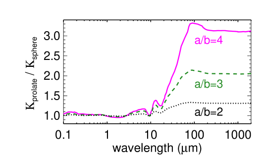
Figure 3: Ratio of the total mass extinction cross section of large prolate and spherical particles with same volume. Prolates, with $a/b$ ratios as labelled, and spheres have same size distribution and relative weights ($w_{i}$) as for dust in the solar neighbourhood (Table 3).

2.8 Element abundances

Estimating the absolute elemental abundances is a tricky task, and in the literature there is no consensus yet as to their precise values. To give one example, for the cosmic (solar or stellar) C/H abundance ratio, expressed in ppm, one finds values of: 417 (Cameron & Fegley 1982), 363 (Anders & Grevesse 1989), 398 (Grevesse et al. 1993), 330 (Grevesse & Sauval 1998), 391 (Holweger 2001), 245 (Asplund & Garcia-Perez 2004), 269 (Asplund et al. 2009), 316 (Caffau et al. 2010), 245 (Lodders 2010), and 214 (Nieva & Przybilla 2012), respectively. Towards 21 sight lines Parvathi et al. (2012) derive C/H ratios between 69 and 414 ppm. Nozawa & Fukugita (2013) consider a solar abundance of C/H = 251 ppm with a scatter between 125 to 500 ppm. For dust models one extra complication appears as one needs to estimate how much of the carbon is depleted from the gas into the grains. Present estimates are that 60% – 70% of all C atoms stick into dust particles (Sofia et al. 2011, Cardelli 1996), whereas earlier values range between 30 – 40 % (Sofia et al. 2004). From extinction fitting, Mulas et al. (2013) derive an average C abundance in grains of $145$ ppm and estimate an uncertainty of about a factor of two. The abundance of O is uncertain within a factor of two. Variations of absolute abundance estimates are noticed for elements such as Si, Mg and Fe, for which one assumes that they are completely condensed (for a recent review on dust abundances see Voshchinnikov et al. 2012). Averaging over all stars of the Voshchinnikov & Henning (2010) sample the total Si abundance is $25\pm 3$ ppm.

We design a dust model where only relative abundances need to be specified. These are the weight factors $w_{i}$ as introduced in Eq. (15). The weight factors prevent us from introducing systematic errors of the absolute dust abundances into the model. Still they can be easily converted into absolute abundances of element $i$ in the dust. We find for the solar neighbourhood a total C abundance of $w_{\rm{C}}=37.2$% (Table  3). To exemplify matters let us assume that the absolute C abundance in dust is $183$ ppm and of Si of $22$ ppm. For this case one converts the weight factors into absolute element abundances of the dust populations to $\Upsilon_{\rm{aC}}=143.5$ ppm, $\Upsilon_{\rm{Si}}=19.1$ ppm, $\Upsilon_{\rm{gr}}=21$ ppm, $\Upsilon_{\rm{sSi}}=2.9$ ppm, $\Upsilon_{\rm{PAHs}}=6.7$ ppm, $\Upsilon_{\rm{PAHb}}=11.5$ ppm, respectively. These numbers can be updated following Eq. 15 and Table 3 whenever more accurate estimates of absolute element abundances in the dust become available.

2.9 Optical thin emission

For optically thin regions we model the emission spectrum of the source computed for 1g of dust at a given temperature. The emission $\epsilon_{i}(r)$ of a dust particle of material $i$ and radius $r$ is

$$\begin{array}[]{r l}\epsilon_{i}(r)=&{\int}{K_{\nu{{,i}}}^{abs}(r)\,J_{\nu}\,\mathrm{d}\nu}\\ &\\ =&{\int}{K_{\nu{{,i}}}^{abs}(r)\,P(r,T)\,B_{\nu}(T)\,\mathrm{d}T\,\mathrm{d}\nu}\,,\end{array}$$ (19)

where the mass absorption cross sections are defined in Eqs. (14, 16), $J_{\nu}$ denotes the mean intensity, $B_{\nu}(T)$ is the Planck function and $P(r,T)$ is the temperature distribution function that gives the probability of finding a particle of material $i$ and radius $r$ at temperature $T$. This function is evaluated using an iterative scheme that is described by Krügel (2008). The $P(T)$ function needs only to be evaluated for small grains as it approaches a $\delta$-function for large particles. The total emission $\epsilon_{\nu}$, is given as sum of the emission $\epsilon_{{i,}\nu}(r)$ of all dust components.

2.10 Dust radiative transfer

For dust enshrouded sources we compute their emission spectrum by solving the radiative transfer problem. Dropping for clarity the frequency dependency of the variables, the radiative transfer equation of the intensity $I$ is

$$I(\tau)=I(0)\ e^{-\tau}\ +\ \int_{0}^{\tau}S(\tau^{\prime})\ e^{-(\tau-\tau^{\prime})}\mathrm{d}\tau^{\prime}\,.$$ (20)

We take as source function

$$S={{K_{\rm{sca}}J+\sum_{i}\epsilon_{i}}\over{K_{\rm{ext}}}}\,,$$ (21)

where $\epsilon_{i}$ is the emission of dust component $i$ computed according to Eq. (19). The problem is solved by ray tracing and with the code described in Krügel (2008). Dust temperatures and $P(T)$ are derived at various distances from the source. The star is placed at the centre of the cloud, and is considered to be spherically symmetric. Our solution of the problem for arbitrary dust geometries is discussed by Heymann & Siebenmorgen (2012).

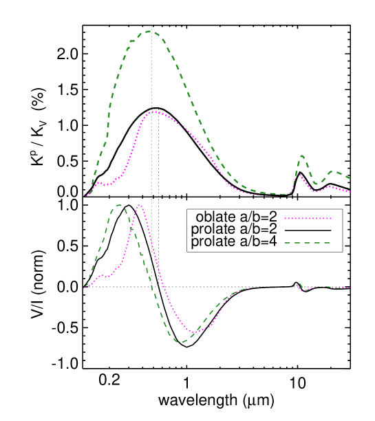
Figure 4: Linear (top) and circular (bottom) polarisation spectra of silicates with $r_{-}=100$ nm, $r_{+}=450$ nm, $q=3.5$. The axial ratios $a/b$ and grain shapes (prolate, oblate) are indicated. The circular polarisation spectra are normalized to their maxima.

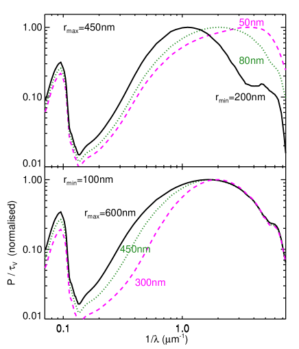
Figure 5: Influence of the upper, $r_{+}$, and lower, $r_{-}$, limit of the particle radii of aligned silicates on the spectral shape of the dichroic polarisation. Shown are prolates with $a/b=2$ and $q=3.5$. Top: $r_{+}$ is held constant at 450 nm and polarisation spectra are computed for $r_{-}=50$, 80, and 200 nm that give rise to a maximum polarisation of $p/\tau_{\rm V}=2.1$%, 1.6%, and 0.8%, respectively. Bottom: lower limit of $r_{-}=100$ nm and varying $r_{+}=300$, 450, and 600 nm that produce a maximum polarisation of $p/\tau_{\rm V}=1.7$%, 1.4%, and 1.2%, respectively.

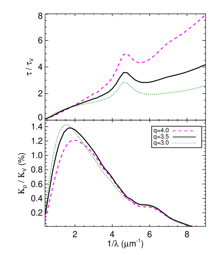
Figure 6: Influence of the exponent of the dust size distribution $q$ on the extinction and linear polarisation curve. For the polarisation we consider prolates made up of silicates with $r_{+}=450$ nm and other parameters as for the solar neighbourhood (Table 3).

2.11 Linear polarisation

Observations of reddened stars frequently show linear polarisation of several percent. These stars have often such thin dust shells, if any, that the polarisation cannot be explained by circumstellar dust (Scicluna et al. 2013). As discussed in Sect. 2.2, partly aligned non–spherical grains have different extinction with respect to their orientation, and therefore they polarise the radiation. The polarisation scales with the amount of dust, hence with the optical depth towards the particular sight line (Eqs. 3, 4). In the model the linear polarisation cross section $K_{\rm{p}}({\nu})$, is computed utilizing ${C}_{{\rm p}}(\nu)$ (Eq. 8) and replacing subscript ext by p in Eqs. (13, 14). Observations of linear polarisation by dichroic extinction are modelled using:

$$p/\tau_{\rm V}=K_{\rm{p}}(\nu)/K_{\rm{ext,V}}\,.$$ (22)

We apply the dust model with the parameters of Table 3, col.2. For grain alignment we assume the IDG mechanism of Eq. (6). We consider moderately elongated particles with $a/b=2$ and assume that only large grains with sufficient inertia are aligned and that grains smaller than about 50 nm are randomly oriented. We show in Fig. 4 that larger axial ratios increase the maximum polarisation and do not influence the spectral shape of the polarisation curve strongly. However, for wavelengths below $\lambda_{\rm{max}}$, one notices that oblate particles have a stronger decline in the polarisation than prolates.

Table 2: Log of FORS spectro-polarimetric observations, all of which were obtained on 2011-01-21.

Target			Linear polarisation				Circular polarisation
Name		PA	grism 600 B		grism 1200 R		grism 600 B		grism 1200 R
		(°)	(hh:mm)	$t$ (sec)	(hh:mm)	$t$ (sec)	(hh:mm)	$t$ (sec)	(hh:mm)	$t$ (sec)
HD 35149	= HR 1770	0	00:24	29	00:44	24	00:49	34	00:52	40
		90	01:38	12	01:21	16	01:47	20	01:29	32
HD 37061	= $\nu$ Ori	30	02:04	40	02:23	40	02:12	85	02:32	101
		60	04:10	60	$\cdots$	$\cdots$	04:17	60	$\cdots$	$\cdots$
		90	03:51	90	$\cdots$	$\cdots$	04:58	60	$\cdots$	$\cdots$
		120	03:08	51	03:27	36	04:18	150	00:00	300
		150	04:28	56	00:00	300	04:35	60	$\cdots$	$\cdots$
		210	02:48	12	00:00	300	02:56	48	$\cdots$	$\cdots$
HD 37903	= BD$-$02 1345	0	04:49	150	05:12	175	05:00	280	05:25	435
		0	05:54	200	06:12	235	06:03	200	06:22	240
HD 93250	= CD$-$58 3537	0	06:47	67	07:07	80	06:59	160	07:19	115
		90	07:36	25	07:57	140	07:46	200	08:05	180
HD 99872	= HR 4425	0	09:16	40	09:37	80	09:22	40	09:30	70
HD 94660	= HR 4263	0	08:27	24	00:00	300	08:34	28	$\cdots$	$\cdots$
Ve 6-23	= Hen 3-248	0	09:00	720	$\cdots$	$\cdots$	$\cdots$	$\cdots$	$\cdots$	$\cdots$

One can see from Fig. 5, that the choice of the lower, $r_{\rm{-}}$, and the upper particle radius $r_{+}$ of aligned grains is sensitive to the curvature of the derived polarisation spectrum. Reducing the lower size limit of aligned grains, $r_{-}$, enhances the polarisation at short wavelengths and increasing upper size limit, $r_{+}$, produces stronger polarisation at longer wavelengths. A similar trend is given by altering the exponent $q$ of the size distribution. For larger $q$ there are smaller particles and the polarisation shifts to shorter wavelengths, the maximum polarisation shrinks and the spectrum broadens. The increase of $r_{\rm{-}}$ and the decrease of $q$ can be associated with the growth of dust grains due to accretion and coagulation processes. Voshchinnikov et al. (2013) find that both mechanisms shift the maximum polarisation to longer wavelengths and narrow the polarisation curve. These characteristics are parameterised by the coefficients $\lambda_{\max}$ and $k_{p}$ of the Serkowski curve Eq. (25), respectively. However, this effect is less pronounced than altering the range of particle sizes of aligned grains. In Fig.6 we show the polarisation curve for $q=3$, 3.5, and 4 of silicates with prolate shape $a/b=2$, $r_{\rm{-}}=100$ nm, $r_{+}=450$ nm using IDG alignment as well as the influence of $q$ on the derived extinction curve. One notices a strong effect in which larger $q$ values produce steeper UV extinction. In summary the extinction is sensitive to variations of $q$ while the polarisation spectrum depends critically on the size spectrum of aligned grains.

The model predicts a strong polarisation in the silicate band (Fig. 5). This is in agreement with the many detections of a polarised signal at that wavelength (Smith et al. 2000). However, in the mid IR two orthogonal mechanisms may be at work and produce the observed linear polarisation. There is either dichroic absorption as discussed in this work and observed in proto-stellar systems (Siebenmorgen & Krügel 2000) or dichroic emission by elongated dust particles as observed on galactic scales (Siebenmorgen et al., 2001).

The angle between the line of sight and the (unsigned) magnetic field is in the limits $0\degr\leq\Omega\leq 90\degr$. We find that the spectral shape of the linear polarisation only marginally depends on $\Omega$, contrary to the maximum of the linear polarisation. The polarisation is strongest for $\Omega=90\degr$. For prolate silicate particles with size distribution and IDG alignment characteristic of the ISM the maximum polarisation decreases for decreasing $\Omega$. For $\Omega=60^{0}$ the polarisation decreases to 60% of that found at maximum, and for $\Omega=30\degr$ further down to $\sim$ 20%. The dependency of $p$ with $\Omega$ is used by Voshchinnikov (2012) to estimate the orientation of the magnetic field in the direction of the polarised source. Unless otherwise stated we use $\Omega=90^{\rm{o}}$.

2.12 Circular polarisation

The dust model also predicts the observed circular polarisation of light (Martin & Campbell 1976, Martin 1978). The circular polarisation spectrum as of Eq. (2) is shown in Fig. 4, normalised to the maximum of $V/I$. We apply the same dust parameters as for the linear polarisation spectrum described above. We note that $V/I$ changes sign at wavelengths close to the position of maximum of the linear polarisation (Voshchinnikov 2004). This may explain many null detections of circular polarisation in the visual part of the spectrum because $\lambda_{\rm{max}}\sim 0.5\mu$m. The local maxima and minima of $V/I$ critically depend on elongation and geometry of the grain: prolate versus oblate. In fact, that circular polarisation can provide new insights into the optical anisotropy of the ISM has been proposed long time ago (van de Hulst 1957, Kemp & Wolstencroft 1972). Typically, for both particle shapes, the maximum of $V/I$ is $\sim 7\times 10^{-5}$ for $a/b=2$, and $\sim 25\times 10^{-5}$ for $a/b=4$. Detecting this amount polarisation is at the very limit of the observational capabilities of the current instrumentation.

3 Spectro-polarimetric observations

Linear and circular spectro-polarimetric observations were obtained with the FORS instrument of the VLT (Appenzeller et al. 1998). Our main goal is to constrain the dust models with ultra-high accuracy polarisation measurements. Stars were selected from the sample provided by Voshchinnikov & Henning (2010). Towards these sight lines linear polarisation was previously detected and extinction curves are available. Targets were chosen based on visibility constraints at the time of the observations. Among the various available grisms, we adopted those with higher resolution. The observed wavelength ranges are 340-610 nm in grism 600 B, and 580-730 nm in grism 1200 R. This grism choice was determined by practical considerations on how to accumulate a very high signal-to-noise ratio (SNR) in the interval range where we expect a change of sign of the circular polarisation. Table 2 gives our target list, the instrument position angle on sky (counted counterclockwise from North to East), the UT at mid exposure, and the total exposure time in seconds for each setting.

Linear polarimetric measurements were obtained by setting the $\lambda/2$ retarder waveplate at position angles 0°, 22$\aas@@fstack{\circ}$5, 45°, and 67$\aas@@fstack{\circ}$5. All circular polarisation measurements were obtained by executing once or twice the sequence with the $\lambda/4$ retarder waveplate at 315°, 45°, 135°, and 225°. Because targets are bright, to minimise risk of saturation we set the slit width to $0\aas@@fstack{\prime\prime}5$; this provides a spectral resolution of $\sim 1500$ and $\sim 4200$ in grism 600 B and 1200 R, respectively. Observations of HD 99872 and Ve 6-23 were performed with a slit width of 1″  providing a spectral resolution of $\sim 800$ and $\sim 1200$ in grism 600 B and 1200 R, respectively. Finally, spectra are rebinned by 256 pixels to achieve the highest possible precision in the continuum. This gives a spectral bin of $\sim 17$ nm and $\sim 10$ nm in grisms 600 B and 1200 R, respectively. It allows us to push the signal-to-noise ratio of the circular polarisation measurements to a level of several tens of thousands over a 10 nm spectral bin.

3.1 Standard stars

To verify the alignment of the polarimetric optics, and to measure the instrumental polarisation, we observed two standard stars: HD 94660 and Ve 6-23. From the circular polarimetric observations of the magnetic star HD 94660 we expected a zero signal in the continuum, and, in spectral lines, a signal consistent with a mean longitudinal magnetic field of about -2 kG (Bagnulo et al. 2002). Indeed we found in the continuum a circular polarisation signal consistent with zero. The magnetic field was measured following the technique described in Bagnulo et al. (2002) on non-rebinned data. We found a value consistent with the one above and concluded that the $\lambda/4$ retarder waveplate was correctly aligned.

In Ve 6-23 we measured a linear polarisation consistent with the expected values of about 7.1 % in the $B$ band, 7.9 % in the $V$ band, and with a position angle of $\sim 173\degr$ and 172° in $B$ and $V$, respectively (Fossati et al. 2007). This demonstrates that the $\lambda/2$ retarder waveplate was correctly set. An unexpected variation of the position angle $\Theta$ is observed at $\lambda\la 400$ nm, possibly related to a substantial drop in the signal-to-noise ratio. Patat & Romaniello (2006) identified such a spurious and asymmetric polarization field that is visible in FORS1 imaging through the B band. We measured the linear polarisation of HD 94660, expecting a very low level in the continuum, and we found a signal of $\sim 0.18$ % that is discussed below.

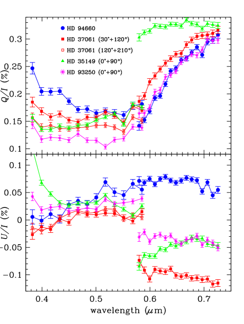
Figure 7: Instrumental linear polarisation spectra derived from observing pairs as labelled together with the continuum polarisation of HD 94660. Stokes parameters $Q/I$ (top) and $U/I$ (bottom) are measured with respect to the instrument reference system.

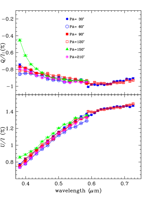
Figure 8: Linear polarisation spectra of HD 37061 that are corrected for instrumental contribution at various PA as labelled. Stokes parameters $Q/I$ (top) and $U$ (bottom) are measured having as a reference direction the celestial meridian passing through the target.

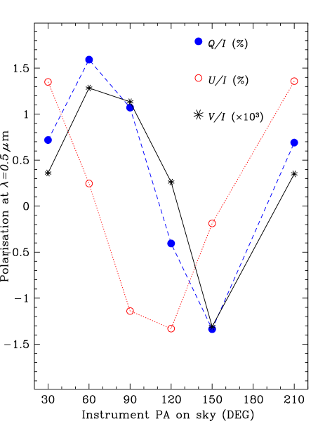
Figure 9: Polarisation at $\lambda=500$ nm of HD 37061 at various instrument position angles. $Q/I$ (blue dashed line) and $U/I$ (red dotted line) are measured in the instrument reference system. The circular polarisation (black solid line) is approximately one tenth of the linear polarisation in the principal plane of the Wollaston prism.

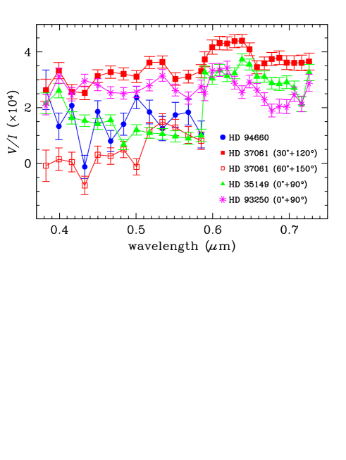
Figure 10: Circular polarisation in the continuum of HD 94660 at instrument PA=$0^{\circ}$ and of other stars from observing pairs as labelled.

3.2 Instrumental linear polarisation

We observed the stars at different instrument position angles on sky to evaluate the instrumental polarisation. The rationale of this observing strategy is that observations of circular polarisation should not depend on the position angle (PA) of the instrument, while linear polarisation measurement follow a well known transformation (see Eq. (10) in Bagnulo et al. 2009). For example, denoting with $P_{Q}^{(\alpha)}$, $P_{U}^{(\alpha)}$, $P_{V}^{(\alpha)}$ the reduced Stokes parameters measured with the instrument position at PA= $\alpha$ on sky, one should find:

$$\begin{array}[]{rcl}P_{Q}^{(90)}&=&-P_{Q}^{(0)}\\[5.69054pt] P_{U}^{(90)}&=&-P_{U}^{(0)}\\[5.69054pt] P_{V}^{(90)}&=&P_{V}^{(0)}\;.\\ \end{array}$$ (23)

Departures from this behaviour may be due to spurious instrumental effects, which should not change as the instrument rotates. Hough et al. (2007) suggest to evaluate the instrumental linear polarisation as

$$\begin{array}[]{rcl}P_{Q}^{\rm instr}&=&\frac{1}{2}\,\left(P_{Q}^{(0)}-P_{Q}^{(90)}\right)\\ P_{U}^{\rm instr}&=&\frac{1}{2}\,\left(P_{U}^{(0)}-P_{U}^{(90)}\right)\,.\\ \end{array}$$ (24)

Instrumental polarisation of $\sim 0.1$ % is identified in FORS1 data by Fossati et al. (2007), and is discussed by Bagnulo (2011). From the analysis of our data we confirm that FORS2 measurements are affected by an instrumental polarisation that depends on the adopted grism. By combining the measurements of HD 37061 obtained at instrument position angles 30° and 120° in grism 600 B, we measure a spurious signal of linear polarisation of about $0.16$ % that is nearly constant with wavelength along the principal plane of the Wollaston prism. In grism 1200 R, we find that the instrumental contribution in the principal plane of the Wollaston prism is linearly changing with wavelength from $\sim 0.2$ % at $\lambda=580$ nm to $\sim 0.32$ % at $\lambda=720$ nm; and in the perpendicular plane we find a value $\sim-0.1$ % that is nearly constant with wavelength (Fig. 7). From the observations of the same star obtained at instrument position angles 120° and 210° (grism 600 B only) we retrieve $\sim 0.14$ % in the principal plane of the Wollaston prism. Similar values of the instrumental polarisation are derived for the observations of the other two targets that are shown in Fig. 7. A higher instrumental polarisation is observed at $\lambda\la 400$ nm than at longer wavelengths.

We conclude that the instrumental polarisation is either not constant in time or depends on the telescope pointing. It is, at least in part, related to the grism, and is much higher and wavelength dependent in in the measurements obtained with the holographic grism 1200 R than in those obtained with grism 600 B. We note that holographic grisms are known to have a transmission that strongly depends on the polarisation of the incoming radiation. Nevertheless, the instrumental polarisation may depend also on the telescope optics and the position of the Longitudinal Atmospheric Dispersion Corrector (LADC, Avila et al. 1997). Our experiments to measure the instrumental polarisation by observing at different PA suggest that the linear polarisation signal measured in HD 94660 is at most instrumental (Fig. 7).

Figure 8 shows all our measurements of HD 37061 obtained at various instrument PA and corrected for our estimated instrumental polarisation. All these spectra refer to the north celestial meridian. These data show that, although the photon noise in a spectral bin of 10 nm is well below 0.01 %, the accuracy of our linear polarisation measurements is limited by an instrumental effect that we have calibrated probably to within $\sim 0.05$ %.

3.3 Instrumental circular polarisation

In our science targets, we also find that circular polarisation measurements depend on the instrument PA. The fact that a zero circular polarisation is measured in the continuum of HD 94660, a star not linearly polarised, suggests that the cross-talk from intensity $I$ to Stokes $V$ is negligible, and that the spurious circular polarisation is due to cross-talk from linear to circular polarisation. The observations of HD 37061 strongly support this hypothesis, as the measured circular polarisation seems roughly proportional to the $Q/I$ value measured in the instrument reference system (Fig. 9). This phenomenon is discussed by Bagnulo et al. (2009). It can be physically ascribed either to the instrument collimator or the LADC. If cross-talk is stable, the polarisation intrinsic to the source can be obtained by averaging the signals measured at two instrument PAs that differ by 90°, i.e., using exactly the same method adopted for linear polarisation. For HD 37061, with grism 600 B, the average signal is $(P_{V}^{(30)}+P_{V}^{(120)})/2\sim 0.03$ % (Fig. 10). By combining the pairs of observations at 120° and 210° we find $\sim 0.1$ %. Therefore the cross-talk from linear to circular polarisation is not constant with time, telescope or instrument position. In grisms 1200 R we obtain $(P_{V}^{(30)}+P_{V}^{(120)})/2\sim 0.03$ %. In Fig. 10 we also show the measurements in grism 600 B towards HD 35149 giving $(P_{V}^{(0)}+P_{V}^{(90)})/2\sim 0.05$ % and towards HD 93250 of $\sim 0.02$ %, respectively.

Our observing strategy reduces the cross-talk from linear to circular polarisation. Nevertheless, the instrumental issues require a more accurate calibration. We are able to achieve in the continuum of the circular polarisation spectrum an accuracy of $\sim 0.03$ %. This is, however, insufficient to test the theoretical predictions computed in Fig. 4. Linear polarisation spectra that are corrected for instrumental signatures of the stars HD 37061 (Fig. 12), HD 93250 (Fig. 13), HD 99872 (Fig. 14), and HD 37903 (Fig. 15) are discussed below.

4 Fitting results

The dust model is applied to average properties of the ISM and towards specific sight-lines. We set-up models so that abundance constraints are respected to within their uncertainties (Sect. 2.8), and we fit extinction, polarisation and emission spectra. The observed extinction is a line-of-sight measurement to the star, while the IR emission is integrated over a larger solid angle and along the entire line-of-sight through the Galaxy. In principle both measurements treat different dust column densities. Therefore an extra assumption is made that the dust responsible for extinction and emission has similar physical characteristics. Dust emission from dense and cold background regions may give a significant contribution to the FIR/submm. However, PAH are mostly excited by UV photons that cannot be emitted far away from the source, and the same holds for warm dust that needs heating by a nearby source.

4.1 Dust in the solar neighbourhood

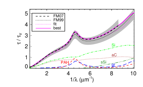
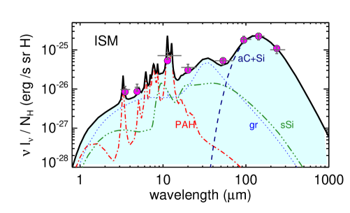
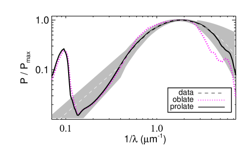
Figure 11: Dust in the solar neighbourhood. Mean (dashed) and 1$\sigma$ variation (hatched area) of the observed extinction curves in the ISM, (up to 8.6 $\mu$m^-1 by Fitzpatrick (1999) and $\leq 10$ $\mu$m^-1 by Fitzpatrick & Massa (2007)). The contribution of the individual dust components to the total extinction of the model with scaled (magenta line) and unscaled (magenta dotted) cross sections (Eq. 17) are given (top). Emission normalized per H atom when dust is heated by the ISRF. High Galactic latitudes observations with $1\sigma$ error bars (gray) from DIRBE (Arendt et al. 1998) and FIRAS (Finkbeiner et al. 1999). The model fluxes convolved with the band passes of the observations are shown as filled circles. The contribution of the dust components to the total emission (black line) is shown (middle). Mean (dashed) and 1$\sigma$ variation (hatched area) of the observed linear polarisation normalised to the maximum polarisation as given by Voshchinnikov et al. (2012). The normalised linear polarisation of silicates with prolate (black line) and oblate (magenta dotted) shapes is shown (bottom).

The average of the extinction curves over many sight lines is taken to be representative for the diffuse ISM of the Milky Way and gives $R_{\rm{V}}=3.1$. Such average extinction curves and their scatter are given by Fitzpatrick (1999) up to 8.6$\mu$m^-1 and Fitzpatrick & Massa (2007) up to 10$\mu$m^-1. They are displayed in Fig. 11 as a ratio of the optical depths. The average extinction curve is approximated by varying the exponent of the dust size distribution $q$ and the relative weights $w_{i}$ of the dust populations. The upper size limit of large grains is derived by fitting the mean polarisation spectrum of the Milky Way discussed below. We find $r_{+}=0.45\mu$m. In 1 g of dust we choose: 546 mg to be in large silicates, 292 mg in amorphous carbon, 43 mg in graphite, 82 mg in small silicates, 14 mg in small and 23 mg in large PAHs, respectively. A fit that is consistent to within the errors of the mean extinction curve is derived with the parameters of Table 3 and is shown in Fig. 11.

Comparing results of the extinction fitting with infrared observations at high galactic latitudes has become a kind of benchmark for models that aim to reproduce dust emission spectra of the diffuse ISM in the Milky Way (Désert et al. 1990; Siebenmorgen & Krügel 1992; Dwek et al. 1997; Li& Draine 2001; Compiegne et al. 2011; Robitaille et al. 2012). In these models the dust is heated by the mean intensity, $J_{\nu}^{\rm{ISRF}}$, of the interstellar radiation field in the solar neighbourhood (Mathis et al. 1983). Observations at Galactic latitude $|b|\ga 25\degr$ using DIRBE (Arendt et al. 1998) and FIRAS (Finkbeiner et al. 1999) on board of COBE are given in $\lambda I_{\lambda}/N_{\rm H}$ (erg/s/sr/H-atom), with hydrogen column density $N_{\rm H}$ (H-atom/cm²). Therefore we need to convert the units and scale the dust emission spectrum computed by Eq. (19) by the dust mass $m_{d}$ (g–dust/H-atom); this gives $I_{\lambda}/N_{\rm H}=m_{d}\ \epsilon_{\lambda}$.

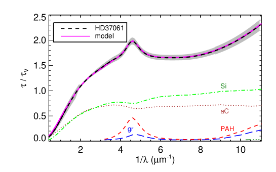
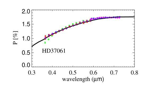
Figure 12: Extinction curve (top) and polarised spectrum (bottom) of HD 37061. The observed extinction curve (black dashed line) with 1 $\sigma$ error bars (hatched area) and the dust model (magenta solid line) with contribution from individual dust components are shown as labelled. The FORS2 linear polarisation spectra (circles) and the model (black solid line) is shown. Model parameters are given in Table 3.

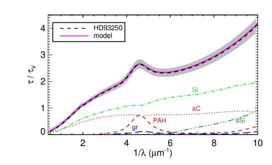
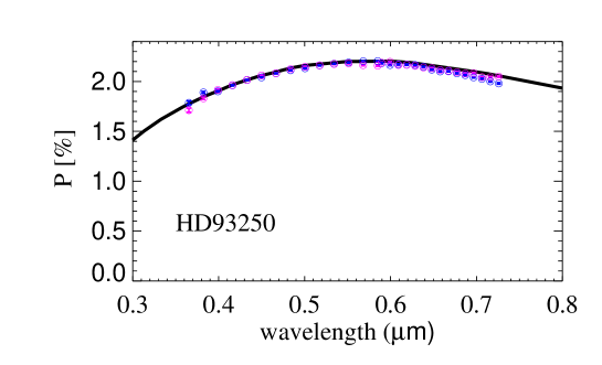
Figure 13: Same as Fig.12 for HD 93250.

We derive the conversion factor by matching the model flux to that in the 140$\mu$m DIRBE band pass. This gives $m_{\rm d}=1.48\times 10^{-26}$ (g-dust/H-atom) and a gas–to–dust mass ratio towards that direction of $(1.36\ m_{\rm p}/m_{\rm d})\sim 153$. If one corrects for the different specific densities $\rho_{i}$ of the dust materials, our estimate is consistent within 8% of that by Li & Draine (2001). A Kramers–Kronig analysis is applied by Purcell (1969) finding as principle value an upper limit of $1.36\ m_{\rm p}/m_{\rm d}<170$, where a specific density of the dust material of $\rho\leq 2.5$ (g/cm³) and a correction factor of 0.95 for the grain shape is assumed (cmp. Eq. (21.17) in Draine 2011). The dust mass in the model shall be taken as a lower limit because there could be undetected dust components made up of heavy metals. For example, a remaining part of Fe that is not embedded into the amorphous olivines (Voshchinnikov et al. 2012) might be physically bonded in layers of iron-fullerene clusters (Fe$\cdot$C₆₀, Lityaeva et al., 2006) or other iron nanoparticles (Draine & Hensley 2013). To our knowledge there is no firm spectral signature of such putative components established so we do not consider them here. Nevertheless, in the discussion of the uncertainty of $m_{d}$ one should consider the observational uncertainties in estimates of $N_{\rm H}$ towards that region as well.

The total emission and the spectrum of each grain population is shown in Fig. 11. All observed in-band fluxes are fit within the uncertainties. We compare the dust emission computed by applying cross sections of the initial physical model with that of the fine-tuned cross sections (Eq. 17). We find that the difference of these models in the DIRBE band pass is less than 1%. The graphite emission peaks in the 20–40$\mu$m region. This local maximum in the emission is due to the optical constants. We verified that the emission by graphite in that region becomes flatter when applying different optical constants of graphite, such as those provided by Laor & Draine (1993) and Draine & Lee (1984). Such flatter graphite emission is shown by e.g., Siebenmorgen & Krügel (1992). The 12$\mu$m DIRBE band is dominated by the emission of the PAHs. We have difficulties to fit this band by adopting PAH cross sections as derived for starburst nuclei. Li & Draine (2001) underestimate the emission in this DIRBE band by 40%. In their model the 11.3 and 12.7$\mu$m bands do not depend on the ionisation degree. In the laboratory it is observed that the ratio of the C-H stretching bands, at 11.3 and 12.7$\mu$m, over the C=C stretching vibrations, at 6.2 and 7.7$\mu$m, decrease manifold upon ionisation (Tielens 2008). Therefore in the diffuse ISM we vary the PAH cross section as compared to the ones derived in the harsh environment of OB stars where PAHs are likely to be ionised (Table 1). Data may be explained without small silicates.

In the optical and near IR the observed polarisation spectra of the ISM can be fit by a mathematical formulae, known as the Serkowski (1973) curve:

$$\frac{p(\lambda)}{p_{\max}}=\exp\left[-k_{p}\ \ln^{2}\left(\frac{\lambda_{\max}}{\lambda}\right)\right]\,,$$ (25)

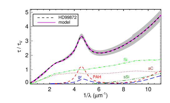
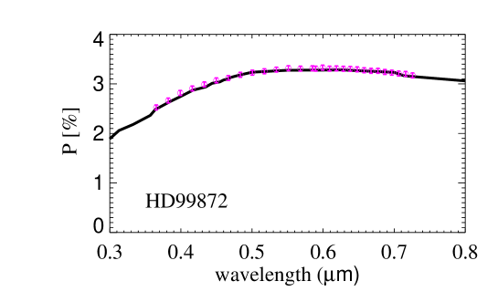
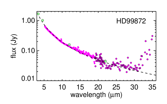
Figure 14: Top and middle panels as in Fig.12 for HD 37061. Bottom: 3 – 36 $\mu$m emission observed with Spitzer/IRS (red filled circles) and WISE (green filled circles). The photospheric emission of the star is represented by the dashed line

where the maximum polarisation is observed to be $p_{\rm{max}}/A_{V}\la 3\%/$mag (Whittet 2003). In the thermal IR at $\lambda>2.5\,\mu$m polarisation data are fit by a power–law where $p(\lambda)\propto\lambda^{-t}$ with $1.6\leq t\leq 2$ (Martin et al., 1992, Nishiyama et al. 2006). This fit naturally breaks down in the 10$\mu$m silicate band. The average observed linear polarisation of the ISM is displayed in Fig. 11. The Serkowski curve is fit without carbon particles, only silicates are aligned. We find a good fit assuming that silicates with particle sizes of radii between 100 – 450 nm are aligned. Below 0.3$\mu$m the mean polarisation spectrum is better explained by dust of prolate than oblate structure (Fig. 11).

4.2 HD 37061

We repeat the exercise of the Sect. 4.1 and model extinction, polarisation and, when available, dust emission spectra. So far we modelled dust properties from extinction and polarisation data when observations are averaged over various sight lines. In the following we fit data towards a particular star and choose those for which we present observations of the linear polarisation spectrum.

This star is of spectral type B1.5V, and located at 720 pc from us. The extinction curve is compiled by Fitzpatrick & Massa (2007). The selective extinction is $R_{\rm V}=4.55\pm 0.13$ and the visual extinction $A_{\rm V}=2.41\pm 0.11$ (Voshchinnikov et al. 2012). ISO and Spitzer spectra of the dust emission are not available. Polarisation spectra are observed by us with of FORS/VLT. The spectra are consistent with earlier measurements of the maximum linear polarisation of $p_{\rm{max}}=1.54\pm 0.2$ % at $\lambda_{\rm{max}}=0.64\pm 0.04\,\mu$m by Serkowski et al. (1975). A fit to the extinction curve and the polarisation spectrum is shown in Fig. 12. The observed polarisation spectrum is fit by silicate grains that are of prolate shape with IDG alignment and $\Omega\sim 55^{\rm{o}}$, other parameters as of Table 3.

4.3 HD 93250

This star is of spectral type O6V and located 1.25 kpc from us. The extinction curve is compiled by Fitzpatrick & Massa (2007) and between $3.3\mu\rm{m}^{-1}\la\lambda^{-1}\la 11\mu\rm{m}^{-1}$ by Gordon et al. (2009), who present spectra of the Far Ultraviolet Spectroscopic Explorer (FUSE) and supplemented spectra from the International Ultraviolet Explorer (IUE). The selective extinction is $R_{\rm V}=3.55\pm 0.34$ and the visual extinction $A_{\rm V}=1.54\pm 0.1$ (Gordon et al. 2009). Polarisation spectra are observed by us in two orientations of the instrument; other polarisation data as well as ISO or Spitzer spectra are not available. A fit to the extinction curve and the polarisation spectrum is shown in Fig. 13. Dust parameters are summarised in Table 3.

4.4 HD 99872

The star has spectral type B3V and is located at 230 pc from us. The extinction curve is compiled by Fitzpatrick & Massa (2007) and between $3.3\mu\rm{m}^{-1}\la\lambda^{-1}\la 11\mu\rm{m}^{-1}$ by Gordon et al. (2009). The selective extinction is $R_{\rm V}=2.95\pm 0.44$ and the visual extinction $A_{\rm V}=1.07\pm 0.04$ (Gordon et al. 2009). The spectral shape of the FORS polarisation can be fit by adopting aligned silicate particles with a prolate shape, while a contribution of aligned carbon grains is not required. The observed maximum polarisation of 3.3 % is reproduced assuming IDG alignment with efficiency computed by Eq.(6) and $a/b\sim 6$. Dust parameters are summarised in Table 3. A fit to the extinction curve, polarisation spectrum, and IR emission is shown in Fig. 14. The IR emission is constrained by WISE (Cutri et al. 2012) and by photometry and a Spitzer/IRS archival spectrum (Houck et al. 2004). The 3 – 32$\mu$m observations are consistent with a 20000 K blackbody stellar spectrum, and do not reveal spectral features by dust. At wavelengths $\ga 32\,\mu$m the observed flux is in excess of the photospheric emission. The excess has such a steep rise that it is not likely to be explained by free–free emission. It is pointing towards emission from a cold dust component such as a background source or a faint circumstellar dust halo. The optical depth of such a putative halo is too small to contribute to the observed polarisation that is therefore of interstellar origin (Scicluna et al. 2013). Unfortunately it has not been possible to find in the literature high quality data at longer wavelengths to confirm and better constrain the far IR excess.

5 The Reflection Nebula NGC 2023

We present observations towards the star HD 37903, which is the primary heating source of the reflection nebula NGC 2023. It is located in the Orion Nebula at a distance of $\sim 400$ pc (Menten et al. 2007). The star is of spectral type B1.5V. It has carved a quasi–spherical dust–free HII region of radius of $\leq 0.04$ pc (Knapp et al. 1975, Harvey et al. 1980). Dust emission is detected further out, up to several arcmin, and is distributed in a kind of bubble–like geometry (Peeters et al. 2012). In that envelope ensembles of dust clumps, filaments and a bright southern ridge are noted in near IR and HST images (Sheffer et al. 2011).

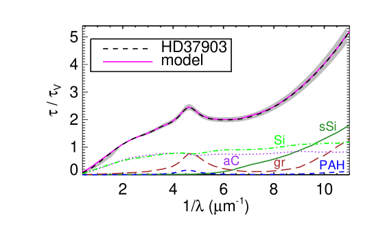
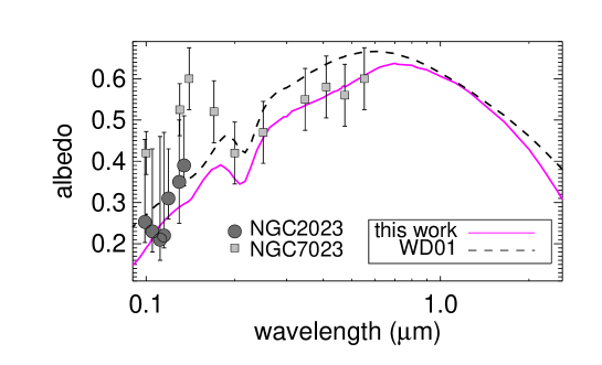
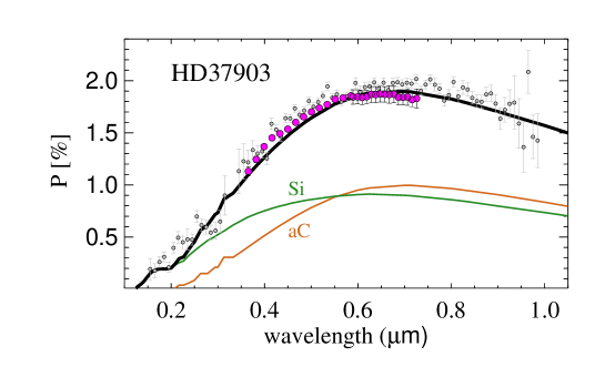
Figure 15: Extinction (top, with notation of Fig. 12.), albedo (middle) and linear polarisation spectrum (bottom) of HD 37903. The albedo of the dust model of this work (magenta line) and by Weingartner & Draine (2001, dashed) is displayed together with estimates of the dust albedo of the reflection nebulae NGC 7023 (square) and NGC 2023 (circle). The observed polarisation spectrum with 1$\sigma$ error bars of this work (red symbols) and as compiled by Efimov (2009, gray symbols) is displayed together with the model (black line) that is the sum of aligned silicates (green) and amorphous carbon (orange) particles. Dust parameters are summarised in Table 3.

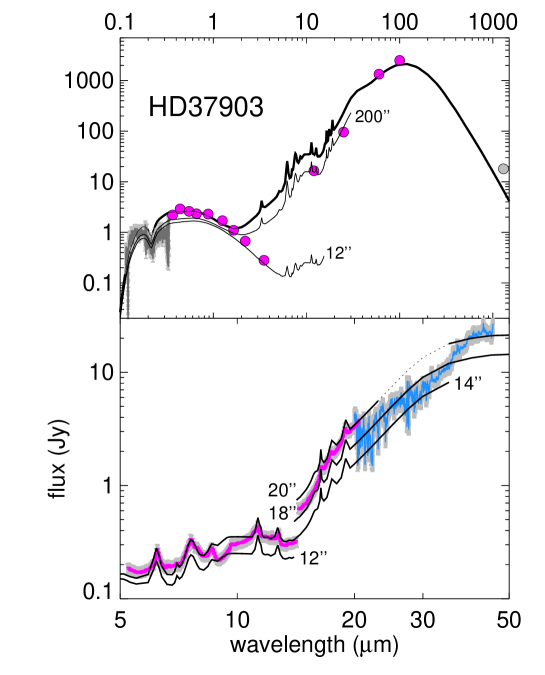
Figure 16: Spectral energy distribution of HD 37903 that is heating NGC 2023 (top) is shown together with a zoom into the 5 – 50 $\mu$m region (bottom): photometric data (symbols); spectra by IUE (dark gray), Spitzer/IRS (magenta) and ISOSWS (blue) with 1$\sigma$ error (gray hatched area) and the model (black lines) in apertures as indicated.

5.1 Extinction

The extinction curve towards HD 37903 is observed by Fitzpatrick & Massa (2007) and Gordon et al. (2009). The extinction towards HD 37903 is low and estimates range between A${}_{\rm V}\sim 1.2-1.5$ mag (Burgh et al. 2002, Compiegne et al. 2008, Gordon et al. 2009). The selective extinction is $R_{\rm V}=4.11\pm 0.44$ (Gordon et al. 2009). We fit the extinction curve with parameters as of Table. 3. The resulting fit together with the contribution of the various grain populations is shown in Fig. 15.

The total amount of energy removed by dust from the impinging light beam is equal to (1-$\Lambda$), i.e. it is related to the particle albedo $\Lambda$ (Eq. 18) and the angular distribution of scattered light. The latter is determined by the asymmetry parameter $g$. The albedo and the asymmetry parameter cannot be derived separately and are only observed in a combined form (Voshchinnikov, 2002). These two quantities have been estimated for several reflection nebulae in the Galaxy (Gordon 2004). Reflection nebulae are bright and often heated by a single star. By assuming a simple scattering geometry estimates of $\Lambda$ are given for the reflection nebula NGC 2023 (Burgh et al. 2002) and NGC 7023 (Witt et al. 1982, Witt et al. 1993). They are shown in Fig. 15 together with our dust model of HD 37903 and for comparison the $R_{\rm V}=3.1$ model by Weingartner & Draine (2001). The albedo of both dust models are similar. They are consistent within $1\sigma$ uncertainties of the data of NGC 2023, however deviate with the peak observed at 0.14$\mu$m for NGC 7023.

5.2 Dust envelope

PAH emission of NGC 2023 is detected by Sellgren (1985), with ISOCAM by Cesarsky et al. (2000) and Spitzer/IRS by Joblin et al. (2005). Emission features at 7.04, 17.4 and 18.9 $\mu$m are detected and assigned to neutral fullerene (C₆₀) with an abundance estimate of $<1$% of interstellar carbon (Sellgren et al. 2010). The fullerene show a spatial distribution distinct from that of the PAH emission (Peeters et al. 2012). The dust emission between 5 – 35 $\mu$m in the northern part of the nebula is modelled by Compiegne et al. (2008), who apply a dust model fitting the mean extinction curve of the ISM. The authors approximate that part of the object in a plane parallel geometry and simplify the treatment of scattering. Compiegne et al. (2008) find that the relative weight and hence abundance of PAHs is five times smaller in the denser part of the cloud than in the diffuse ISM.

We compile the spectral energy distribution (SED) towards HD 37903 using photometry in the optical, UBVRI bands by Comeron (2003), in the near-infrared, IJHKL filters by Burgh et al. (2002), IRAS (Neugebauer et al. 1984; Joint IRAS Science 1994) and at 1.3mm by Chini et al. (1984). The SED is complimented by spectroscopy between 0.115$\,\mu$m and 0.32 $\mu$m using data of the International Ultraviolet Explorer (IUE), as available in the Mikulski archive for space telescopes¹, the Spitzer/IRS archival spectrum (Houck et al. 2004) and ISO/SWS spectroscopy (Sloan et al. 2003). The observed SED is shown in Fig. 16.

The observed bolometric IR luminosity is used as an approximation of the stellar luminosity of $L_{*}\sim 10^{4}$L_⊙. We take a blackbody as stellar spectrum. Its temperature of $T_{*}=21000$ K is derived by fitting the IUE spectrum and optical, NIR photometry first in a dust-free model and correcting for a foreground extinction of $\tau\sim D/1kpc=0.4$. Both parameters, $L_{*}$ and $T_{*}$, are appropriate to the spectral type of HD 37903. A weak decline of the dust density with radius is assumed in the models by Witt et al. (1984). We assume in the nebulae a constant dust density of $\rho=10^{-23}$ g/cm³ for simplicity. The inner radius of the dust shell is set at $r_{\rm{in}}=10^{17}$ cm. For the adopted outer radius of $r_{\rm{out}}=1$ pc the total dust mass in the envelope is $M_{\rm{dust}}=0.62$ M_⊙ and the optical depth, measured between $r_{\rm{in}}$ and $r_{\rm{out}}$, is $\tau_{\rm V}=0.8$. We build up SEDs of the cloud within apertures of different angular sizes. The models are compared to the observations in Fig. 16. The 1.3 mm flux is taken as upper limit as it might be dominated by cold dust emission of the molecular cloud behind the nebula. Model fluxes computed for different diaphragms envelope reasonably well data obtained at various apertures.

Fullerenes are not treated as an individual dust component. The cross sections of the PAH emission bands are varied to better fit the Spitzer/IRS spectrum. They are listed in Table 1 and are close to the ones estimated for starburst galaxies. The cross sections of the C-H bands at 11.3 and 12.7 $\mu$m are much smaller and of the C=C vibrations at 6.2 and 7.7 $\mu$m slightly larger than those derived for the solar neighbourhood. This finding is consistent with a picture of dominant emission by ionised PAHs near B stars and neutral PAHs in the diffuse medium. We note that alternatively, the hydrogenation coverage of PAHs can be used in explaining a good part of observed variations of PAH band ratios in various galactic and extra–galactic objects (Siebenmorgen & Heymann, 2012). We do not find a good fit to the 10 $\mu$m continuum emission if we ignore the contribution of small silicate grains.

Table 3: Parameters of the dust models.

Parameter a	Solar	HD 37061	HD 93250	HD 99872	HD 37903
	neighbourhood				(NGC 2023)
$r_{+}$ (nm)	440	485	380	400	485
$r_{\rm{-}}$ (nm)	100	125	100	140	120
$q$	3.4	3.0	3.3	3.3	3.2
$a/b$	2	2	2.2	6	2
$w_{\rm{aC}}$	29.2	40.1	28.8	31.5	34.3
$w_{\rm{Si}}$	54.6	56.2	58.2	55.1	48.1
$w_{\rm{gr}}$	4.3	1.0	0.8	2.4	5.7
$w_{\rm{sSi}}$	8.2	0.3	8.9	5.4	11.2
$w_{\rm{PAHs}}$	1.4	0.8	1.3	2.4	0.2
$w_{\rm{PAHb}}$	2.3	1.6	1.9	3.2	0.5

Notes. ^a Upper ($r_{+}$) and lower ($r_{\rm{-}}$) particle radius of aligned grains, exponent of the dust size distribution ($q$), axial ratio of the particles ($a/b$), and relative weight per g–dust (%) of amorphous carbon ($w_{\rm{aC}}$), large silicates ($w_{\rm{Si}}$), graphite ($w_{\rm{gr}}$), small silicates ($w_{\rm{sSi}}$), small ($w_{\rm{PAHs}}$) and large ($w_{\rm{PAHb}}$) PAHs, respectively.

5.3 Polarisation

Spectro–polarimetric data acquired with the polarimeters on board the WUPPE and HPOL satellites and from ground (Anderson et al. 1996) are compiled by Efimov (2009). They agree to within the errors of the polarisation spectra observed by us with FORS2/VLT. We find a good fit to the polarisation spectrum only when both silicates and amorphous carbon are aligned. The observed polarisation spectrum is fit by grains that are of prolate shape, $\Omega\sim 65\degr$ and other parameters as of Table 3.

As most of the extinction towards HD 37903 is coming from the nebula, one may also consider other alignment mechanisms of the grains such as the radiative torque alignment proposed by Lazarian (2007). Another way to explain the observed polarisation could be due to dust scattering. This would require significant inhomogeneities of the dust density distribution of the nebula within the aperture of the instruments. The contribution of scattering to the polarisation might be estimated from a polarisation spectrum of a nearby star outside the reflection nebula that is not surrounded by circumstellar dust.

6 Conclusion

The main results of this paper are as follows:

1) We have presented an interstellar dust model that includes a population of carbon and silicate grains with a power–law size distribution ranging from the molecular domain (5Å) up to 500 nm. Small grains are graphite, silicates and PAHs, and large spheroidal grains are made of amorphous carbon and silicates. The relative weight of each dust component is specified, so that absolute abundances of the chemical elements are not direct input parameters and used as a consistency check (Eq. 15). We apply the imperfect Davis–Greenstein alignment mechanism to spheroidal dust particles, which spin and wobble along the magnetic field. Their far IR/submm absorption cross section is a factor 1.5 – 3 larger than spherical grains of identical volume. Mass estimates derived from submillimeter observations that ignore this effect are overestimated by the same amount. The physical model fits observed extinction curves to within a few percent and a perfect match is found after fine adjustment of the computed cross sections (Eq. 17).

2) The wavelength-dependent absorption cross-section of PAHs have been revised to give better agreement with recent laboratory and theoretical work. PAH cross-sections of the emission bands are calibrated to match observations in different radiation environments. We have found that in harsh environments, such as in starbursts, the integrated cross-section of the C=C bands at 6.2 and 7.7 $\mu$m are a factor $\sim 2$ larger, and for the C–H bands at 11.3 and 12.7 $\mu$m a factor $\sim 5$ weaker than in the neutral regions of the ISM. The cross sections near OB stars are similar to the ones derived for starbursts.

3) With the FORS instrument of the VLT, we have obtained new ultra-high signal-to-noise linear and circular spectro-polarimetric observations for a selected sample of sight lines. We have performed a detailed study of the instrumental polarisation in an attempt to achieve the highest possible accuracy. We show that circular polarisation provides a diagnostic on grain shape and elongation. However, it is beyond the limit of the observations that we have obtained.

4) The dust model reproduces extinction, linear and circular polarisation curves and emission spectra of the diffuse ISM. It is set up to keep the number of key parameters to a minimum (Table 3). The model accounts for IR observations at high galactic latitudes. It can be taken as representative of the local dust in the solar neighbourhood.

5) We have applied our dust model on individual sight lines ranging between $1.2\la A_{\rm V}/{\rm{mag}}\la 2.4$ and $2.9\la R_{\rm V}\la 4.6$, towards the early type stars: HD 37061, HD 37903, HD 93250, and HD 99872. For these stars we present polarisation spectra and measure a maximum polarisation of 1 – 3 %. The IR emission of the star HD 37903 that is heating the reflection nebula NGC 2023 is computed with a radiative transfer program assuming spherical symmetry. In the Spitzer/IRS spectrum of the massive star HD 99872 we detect an excess emission over its photosphere that is steeply rising towards longer wavelengths and pointing towards a cool dust component.

6) Linear polarisation depends on the type of the spheroid, prolate or oblate, its elongation, and the alignment efficiency. We have found that the spectral shape of the polarisation is critically influenced by the assumed lower and upper radius of dust that is aligned. In conclusion polarisation helps to determine the otherwise purely constrained upper size limit of the dust particles. The observed linear polarisation spectra are better fit by prolate than by oblate grains. For accounting of the polarisation typically only silicates, with an elongation of about 2 and radii between 100 nm and 500 nm need to be aligned.

- (1) [] Allamandola, L.J., Tielens, A.G.G.M., & Barker, J.R. 1985, ApJ, 290, L25
- (2)
- (3) [] Allamandola, L.J., Tielens, A.G.G.M., & Barker, J.R., 1989, ApJS, 71, 733
- (4)
- (5) [] Allamandola, L.J., Hudgins, D.M., Bauschlicher, C.W., Jr., & Langhoff, S.R. 1999, A&A, 352, 659
- (6)
- (7) [] Anders, E., & Grevesse, N. 1989, GeCoA, 53, 197
- (8)
- (9) [] Anderson, C.M., Weitenback, A.J., Code, A.D., Nordsieck, K.H., Meade, M.R., et al. 1996, AJ, 112, 2726
- (10)
- (11) [] Appenzeller, I., Fricke, K., Furtig, W., et al. 1998, The Messenger, 94, 1
- (12)
- (13) [] Arendt, R.G., Odegard, N., Weiland, J.L., et al. 1998, ApJ, 508, 74
- (14)
- (15) [] Asplund, M., & Garcia-Perez, A. E. 2001, A&A, 372, 601
- (16)
- (17) [] Asplund, M., Grevesse, N., Sauval, A.J., & Scott, P. 2009 ARA&A, 47, 481
- (18)
- (19) [] Avila, G., Rupprecht, G., & Beckers, J.M., 1997, SPIE, 2871, 1135
- (20)
- (21) [] Bagnulo, S., 2011. Stellar spectropolarimetry: basic principles, observing strategies, and diagnostics of magnetic fields. In: “Polarimetric Detection, Characterization and Remote Sensing”, Mishchenko, M.I., Yatskiv, Y.S., Rosenbush, V.K., and Videen, G. (eds.) NATO Science for Peace and Security Series C: Environmental Security. Springer
- (22)
- (23) [] Bagnulo, S., Szeifert, T., Wade, G.A., Landstreet, J.D., & Mathys, G. 2002, A&A, 389, 191
- (24)
- (25) [] Bagnulo, S., Landolfi, M., Landstreet, J.D., et al. 2009, PASP, 121, 993
- (26)
- (27) [] Bohren, C.F., & Huffman, D.R. 1983, Absorption and Scattering of Light by Small Particles, John Wiley and Sons, New York
- (28)
- (29) [] Boulanger, F., Baud, B., & van Albada, G.D. 1985, A&A, 144, L9
- (30)
- (31) [] Bouwman, J., Cuppen, H.M., Steglich, M., et al. 2011, A&A, 529, 46
- (32)
- (33) [] Burgh, E.B., Mc Candliss, S.R., & Feldman, P.D. 2002, ApJ, 575, 240
- (34)
- (35) [] Caffau, E., Ludwig, H.-G., Steffen, M., Freytag, B., & Bonifacio, P. 2011, SoPh, 268, 255
- (36)
- (37) [] Cameron, A. G. W., & Fegley, M. B. 1982, Icar, 52, 1
- (38)
- (39) [] Cardelli, J. A., Meyer, D. M., Jura, M., & Savage, B. D. 1996, ApJ, 467, 334
- (40)
- (41) [] Cesarsky, D., Lequeux, J., Ryter, C., & Gérin, M. 2000, A&A, 354, L87
- (42)
- (43) [] Chini, R., Kreysa, E., Mezger, P.G., & Gemünd, H.-P. 1984, A&A, 137, 117
- (44)
- (45) [] Clarke, D. 2010, Stellar Polarimetry, ISBN: 978-3-527-40895-5
- (46)
- (47) [] Cohen, M., Anderson, C. M., Cowley, A., et al. 1975, ApJ, 196, 179
- (48)
- (49) [] Comeron, R.B. 2003, AJ, 125, 2531
- (50)
- (51) [] Compiegne, M., Abergel, A., Verstraete, L., & Habart, E. 2008, A&A, 491, 797
- (52)
- (53) [] Compiegne, M., Verstraete, L., Jones, A., et al. 2011, A&A, 525, 14
- (54)
- (55) [] Cutri, R.M., Skrutskie, M.F., van Dyk, S., et al. 2012, VizieR Online Data Catalog, 2311, 0
- (56)
- (57) [] Das, H.K., Voshchinnikov, N.V., & Ilín, V.B. 2010, MNRAS 404, 625
- (58)
- (59) [] Désert, F.X., Boulanger, F., & Puget, J.L. 1990, A&A, 237, 215
- (60)
- (61) [] Draine, B.T. 2003, ApJ, 598, 1026
- (62)
- (63) [] Draine, B.T. 2011, Physics of the Interstellar and Intergalactic Medium, Princton University Press
- (64)
- (65) [] Draine, B.T., & Lee, H.M. 1984, ApJ, 285, 89
- (66)
- (67) [] Draine, B.T., & Malhotra, S. 1993, ApJ, 414, 632
- (68)
- (69) [] Draine, B.T., & Allaf-Akbari, K. 2006, ApJ, 652, 1318
- (70)
- (71) [] Draine, B.T., & Li, A. 2007, ApJ, 657, 810
- (72)
- (73) [] Draine, B.T., & Fraisse, A.A. 2009, ApJ, 626, 1
- (74)
- (75) [] Draine, B.T., & Hensley, B. 2013, ApJ, 765, 159
- (76)
- (77) [] Dwek, E., Arendt, R.G., Fixsen, D.J., Sodroski, T.J., Odegard, N., et al. 1997, ApJ, 475, 565
- (78)
- (79) [] Efimov, Yu.S. 2009, Bull. CrAO, 105, 82
- (80)
- (81) [] Efstathiou, A., & Siebenmorgen, R., 2009, A&A, 502, 541
- (82)
- (83) [] Finkbeiner, D.P., Davis, M., & Schlegel, D.J. 1999, ApJ, 524, 867
- (84) [] Fitzpatrick, E.L. 1999, PASP, 111, 163
- (85)
- (86) [] Fitzpatrick, E.L., & Massa, D.L. 2007, ApJ, 663, 320
- (87)
- (88) [] Fossati, L., Bagnulo, S., Mason, E., & Landi Degl’Innocenti, E. 2007, ASP, 364, 503
- (89)
- (90) [] Galliano, F., Madden, S.C., & Tielens, A.G.G.M., et al. 2008, ApJ, 679, 310
- (91)
- (92) [] Gordon, K.D. 2004, ASP, 309, 77
- (93)
- (94) [] Gordon, K.D., Cartledge, S., & Clayton, G.C. 2009, ApJ, 705, 1320
- (95)
- (96) [] Greenberg, J.M. 1978, in Cosmic Dust, ed. J.A.M.McDonnell (New York: Wiley), 187
- (97)
- (98) [] Grevesse, N., Noels, A., & Sauval, A. J 1993, A&A, 271, 587
- (99)
- (100) [] Grevesse, N., & Sauval, A. J. 1998, SSRv, 85, 161
- (101)
- (102) [] Guhathakurta, P., & Draine, B.T. 1989, ApJ, 345, 230
- (103)
- (104) [] Guirado, D., Hovenier, J.W., & Moreno, F. 2007, JQSRT, 106, 63
- (105)
- (106) [] Gupta, R., Mukai, T., Vaidya, D.B., Sen, A.K., & Okada, Y. 2005, A&A, 441, 555
- (107)
- (108) [] Harvey, P.M., Thronson, Jr.H.A., & Gatley, I. 1980, ApJ, 235, 894
- (109)
- (110) [] Henning, Th. 2010, ARA&A, 48, 21
- (111)
- (112) [] Heymann, F., & Siebenmorgen, R., 2012 ApJ, 751, 27
- (113)
- (114) [] Holweger, H. 2001, AIPC, 598, 23
- (115)
- (116) [] Hong, S.S., & Greenberg, J.M. 1980, A&A, 88, 194
- (117)
- (118) [] Houck, J.R., Roellig, T.L., van Cleve, J., et al. 2004, ApJS, 154, 18
- (119)
- (120) [] Hough, J.S, Lucas, P. W., Bailey, J. A., & Tamura, M. 2007, ASP, 343, 3
- (121)
- (122) [] Hudgins, D.M., Bauschlicher, C.W., Jr., & Allamandola, L.J. 2005, ApJ, 632, 316
- (123)
- (124) [] Jenkins, E.B. 2009, ApJ, 700, 1299
- (125)
- (126) [] Joblin, C., & Tielens, A.G.G.M. 2011, EAS, 46, 3
- (127)
- (128) [] Joblin, C., Abergel, A., Bernard, J.-P., et al. 2005, IAU 235, 194.
- (129)
- (130) [] Joint IRAS Science 1994, VizieR Online Data Catalog, 2125, 0
- (131)
- (132) [] Kemp, J.C., & Wolstencroft, R.D. 1972, ApJ, 176, L115
- (133)
- (134) [] Kim, S.H., Martin, P.G., & Hendry, P.D. 1994, ApJ, 422, 164
- (135)
- (136) [] Knapp, G.R., Brown, R.L., & Kuiper, T.B.H. 1975, ApJ, 196, 167
- (137)
- (138) [] Krelowski, J. 2002, Adv. Space Res., 30, 1395
- (139)
- (140) [] Krügel, E. 2003, The Physics of Interstellar Dust, IoP, ISBN 0 7503 0861 3
- (141)
- (142) [] Krügel, E. 2008, An introduction to the Physics of Interstellar Dust, IoP, ISBN 978 1 58488 707 2
- (143)
- (144) [] Krügel, E., & Siebenmorgen, R. 1994, A&A, 288, 929.
- (145)
- (146) [] Laor, A., & Draine, B.T. 1993, ApJ, 402, 441
- (147)
- (148) [] Lazarian, A. 2007, JQSRT, 106, 225
- (149)
- (150) [] Li, A., & Draine, B.T. 2001, ApJ, 550, L213
- (151)
- (152) [] Li, A., & Greenberg, J.M. 1997, A&A, 323, 566
- (153)
- (154) [] Lityaeva, I.S., Bulina, N.V., Petrakovskaya, E.A., et al. 2006, Fullerenes, Nanotubes and Carbon Nanostructures, Volume 14, Issue 2-3, pages 499-502.
- (155)
- (156) [] Lodders, K. 2010, Principles and Perspectives in Cosmochemistry, Astronomy and Space Science Proceedings (Berlin: Springer), 379
- (157)
- (158) [] Malloci, G., Mulas, G., Cecchi-Pestellini, C., & Joblin, C. 2008, A&A, 462, 627
- (159)
- (160) [] Malloci, G., Mulas, G., & Mattoni, A. 2011, Chemical Physics, 384, 19
- (161)
- (162) [] Martin, P.G. 1974, ApJ 187, 461
- (163)
- (164) [] Martin, P.G. 1978, Cosmic dust. Its impact on astronomy, Oxford Studies in Physics, Oxford: Clarendon Press
- (165)
- (166) [] Martin, P.G., & Campbell, B. 1976, ApJ, 208, 727
- (167)
- (168) [] Martin, P.G., Adamson, A.J., Whittet, D.C.B., et al. 1992, ApJ, 392, 691
- (169)
- (170) [] Mathis, J.S., Rumpl, W., & Nordsieck, K.H. 1977, ApJ, 217, 425 212
- (171)
- (172) [] Mathis, J.S., Mezger, P.G., & Panagia, N. 1983, A&A, 128, 212
- (173)
- (174) [] Mattioda, A.L., Rutter, L., Parkhill, J., et al. 2008, ApJ, 680, 1243
- (175)
- (176) [] Mennella, V., Baratta, G., & Esposito, A. 2003, ApJ, 587, 727
- (177)
- (178) [] Menten, K.M., Reid, M.J., Forbrich, J., & Brunthaler, A. 2007, A&A, 474, 515
- (179)
- (180) [] Min, M., Waters, L.B.F.M., de Koter, A., et al. 2007, A&A, 462, 667
- (181)
- (182) [] Mishchenko, M.I. 2000, Appl. Opt., 39, 1026
- (183)
- (184) [] Moutou, C., Léger, A., & D’Hendecourt, L. 1996, A&A, 310, 297
- (185)
- (186) [] Mulas, G., Malloci, G., Joblin, C., & Cecchi-Pestellini, C. 2011, EAS, 46, 327
- (187)
- (188) [] Mulas, G., Zonca, A., Casu, S., & Cecchi-Pestellini, C., 2013 ApJS, 207, 7
- (189)
- (190) [] Neugebauer, G., Habing, H.J., van Duinen, R., et al. 1984, ApJ, 278, L1
- (191)
- (192) [] Nieva, M.-F., & Przybilla, N. 2012, A&A, 539, 143
- (193)
- (194) [] Nishiyama, S., Nagata, T., Kusakabe, N., et al. 2006, ApJ, 638, 839
- (195)
- (196) [] Nozawa, T., & Fukugita, M. 2013, ApJ, 770, 13
- (197)
- (198) [] Ossenkopf, V., & Henning, Th. 1994, A&A, 291, 943
- (199)
- (200) [] Parvathi, V.S., Sofia, U.J., Murthy, J., & Babu, S.R.S. 2012, ApJ, 760, 36
- (201)
- (202) [] Patat, N., & Romaniello, M., 2006, PASP, 118, 146
- (203)
- (204) [] Pauzat, F., Talbi, D., & Ellinger, Y. 1997, A&A, 319, 318.
- (205)
- (206) [] Peeters, E., Hony S., & Van Kerckhoven, C. 2002, A&A, 390, 1089
- (207)
- (208) [] Peeters, E., Tielens A.G.G.M, Allamandola, L.J., & Wolfire, M.G. 2012, ApJ, 747, 44
- (209)
- (210) [] Pontoppidan, K.M., Fraser, H.J., Dartois, E., et al. 2003, A&A, 408, 981
- (211)
- (212) [] Puget, J.L., & Léger A. 1989, ARA&A 27, 161
- (213)
- (214) [] Purcell, E.M. 1969, ApJ, 158, 43
- (215)
- (216) [] Robitaille, T.P., Churchwell, E., Benjamin, R.A., et al. 2012, A&A, 545, 39
- (217)
- (218) [] Salama, F., Bakes, E.L.O., Allamandola, L.J., & Tielens, A.G.G.M. 1996, ApJ, 458, 621
- (219)
- (220) [] Scicluna, P., Siebenmorgen, R., & Yakovlev I. 2013, A&A submitted
- (221)
- (222) [] Schutte, W.A., Tielens, A.G.G.M., & Allamandola, L.J. 1993, ApJ, 415, 397
- (223)
- (224) [] Sellgren, K., Allamandola, L., Bregman, J.D., et al. 1985, ApJ, 299, 416
- (225)
- (226) [] Sellgren, K., Werner, M.W., Ingalls, J.G., et al. 2010, ApJ, 722, L54
- (227)
- (228) [] Serkowski, K. 1973, in: Greenberg JM, Hayes DS, editors, Interstellar Dust and Related Topics, Dordrect: Reidel, IAU Symp vol. 52, p. 145
- (229)
- (230) [] Serkowski, K., Mathewson, D.S., & Ford, V.L. 1975, ApJ, 196, 261
- (231)
- (232) [] Sheffer, Y., Wolfire, M., Hollenbach, et al. 2011, ApJ, 741, 45
- (233)
- (234) [] Shurcliff, W.A. 1962, Polarized light. Harvard Univ. Press, Cambridge, 1962
- (235)
- (236) [] Siebenmorgen, R., & Gredel, R. 1997, ApJ, 485, 203
- (237)
- (238) [] Siebenmorgen, R., & Krügel, E. 1992, A&A, 259, 614
- (239)
- (240) [] Siebenmorgen, R., & Krügel, E. 2000, A&A, 364, 625
- (241)
- (242) [] Siebenmorgen, R., Krügel, E., & Laureijs, R. 2001, A&A, 377, 735
- (243)
- (244) [] Siebenmorgen, R., & Krügel, E. 2007, AA, 461, 445.
- (245)
- (246) [] Siebenmorgen, R., & Krügel E. 2010, A&A, 511, 6
- (247)
- (248) [] Siebenmorgen, R., Heymann, F., & Krügel, E. 2011 EAS Publ. Ser., 46, 285
- (249)
- (250) [] Siebenmorgen, R., & Heymann, F. 2012, A&A, 543, 25
- (251)
- (252) [] Sloan, G.C., Kraemer, K.E., Price, S.D., & Shipman, R.F. 2003, ApJS, 147, 379
- (253)
- (254) [] Smith, C.H., Wright, C.M., Aitken, D.K., Roche, P.F., & Hough, J.H. 2000, MNRAS, 312, 327
- (255)
- (256) [] Snow, T.P., & Destree, J.D., 2011, EAS, 46, 343
- (257)
- (258) [] Sofia, U. J., Lauroesch, J. T., Meyer, D. M., & Cartledge, S. I. B. 2004, ApJ, 605, 272
- (259)
- (260) [] Sofia, U. J., Parvathi, V. S., Babu, B. R. S., & Murthy, J. 2011, AJ, 141, 22
- (261)
- (262) [] Tielens, A.G.G.M., 2005, The Physics and Chemistry of the Interstellar Medium, ISBN 0521826349, Cambridge University Press, Sect. 6.4
- (263)
- (264) [] Tielens, A.G.G.M., 2008, ARA&A, 46, 289
- (265)
- (266) [] van Diedenhoven, B., Peeters, E., Van Kerckhoven, C., et al. 2004, ApJ, 611,928
- (267)
- (268) [] van de Hulst, H.C. 1957, Light Scattering by Small Particles,
- (269)
- (270) [] Verstraete, L, & Léger, A. 1992, A&A, 266, 513.
- (271)
- (272) [] Voshchinnikov, N.V. 1989, Astron. Nachr., 31, 265
- (273)
- (274) [] Voshchinnikov, N.V. 2002, Optics of Cosmic Dust, G. Videen and M.Kocifaj (eds.), Kluwer, 2002, p. 1-36
- (275)
- (276) [] Voshchinnikov, N.V. 2004, Astrop. &Sp. Phys. Rev., 12, 1
- (277)
- (278) [] Voshchinnikov, N.V. 2012, JQSRT, 113, 2334
- (279)
- (280) [] Voshchinnikov, N.V. & Farafonov, V.G. 1993, Ap&SS 204, 19
- (281)
- (282) [] Voshchinnikov, N.V. & Das, H.K. 2008, JQSRT, 109, 1527
- (283)
- (284) [] Voshchinnikov, N.V., & Henning, Th. 2010, A&A, 517, A45
- (285)
- (286) [] Voshchinnikov, N.V., Semenov, D.A., & Henning, Th. 1999, A&A, 349, L25
- (287)
- (288) [] Voshchinnikov, N.V., Il’in, V.B., & Henning, Th. 2005, A&A, 429, 371
- (289)
- (290) [] Voshchinnikov, N.V., Henning, Th., Prokopjeva, M.S., & Das, H.K. 2012, A&A, 541, A52
- (291)
- (292) [] Voshchinnikov, N.V., Das, H.K., Yakovlev I.S., Il’in, V.B. 2013, Astron. Lett. Vol. 39, No 7, pp. 421
- (293)
- (294) [] Weingartner, J.C., & Draine, B.T. 2001, ApJ, 548, 296
- (295)
- (296) [] Whittet, D.C.B. 2003, in Dust in the Galactic Environment, Bristol: Institute of Physics Publishing
- (297)
- (298) [] Whittet, D.C.B., Bode, M.F., Longmore, A.J., et al. 1988, MNRAS, 233, 321
- (299)
- (300) [] Witt, A.N., Walker, G.A.H., Bohlin, R.C., & Stecher, T.P. 1982, ApJ, 261, 492
- (301)
- (302) [] Witt A.N., & Schild, R.E. 1986, ApJS, 62, 839
- (303)
- (304) [] Witt, A.N., Petersohn, J.K., Holberg, J.B., Murthy, J., Dring, A., Henry, R.C. 1993, ApJ, 410, 714
- (305)
- (306) [] Witt A.N., & VijH, U.P., 2004, ASP, 309, 115
- (307)
- (308) [] Zonca, A., Cecchi-Pestellini, C., Mulas, G., & Malocci, G. 2011, MNRAS, 410, 1932
- (309)
- (310) [] Zubko, V.G., Mennella, V., Colangeli, L., et al. 1996, MNRAS, 282, 1321
- (311)
- (312) [] Zubko, V., Dwek, E., & Arendt, R.G. 2004, ApJS, 152, 211
- (313)