A Modified Gas-Kinetic Scheme for Turbulent Flow

Abstract

By analogy with the kinetic theory of gases, most turbulence modeling strategies rely on an eddy viscosity to model the unresolved turbulent fluctuations. However, the ratio of unresolved to resolved scales - very much like a degree of rarefaction - is not taken into account by the popular conventional schemes, based on the Navier-Stokes equations. This paper investigates the simulation of turbulent flow with a gas-kinetic scheme. In so doing, the modeling of turbulence becomes part of the numerical scheme: the degree of rarefaction is automatically taken into account; the turbulent stress tensor is not constrained into a linear relation with the strain rate. Instead it is modeled on the basis of the analogy between particles and eddies, without any assumptions on the type of turbulence or flow class. The implementation of a turbulent gas-kinetic scheme into a finite-volume solver is put forward, with turbulent kinetic energy and dissipation supplied by an allied turbulence model. A number of flow cases, challenging for conventional RANS methods, are investigated; results show that the shock-turbulent boundary layer is captured in a much more convincing way by the gas-kinetic scheme.

47.27.em, 47.27.nb, 47.32.Ff, 47.40.Hg, 47.40.Nm , 47.45.Ab, 47.85.Gj, 47.85.ld

1 Introduction

A number of gas-kinetic schemes have been developed over the latest 20 years (refer to [32, 20, 19, 7, 35] and references therein). With respect to conventional CFD, these schemes, derived from the Boltzmann equation, exploit a physically more consistent model of fluid mechanics. Gas-kinetic schemes are more accurate, in particular in the presence of shock waves. Besides, they are more suitable to high-order reconstruction (refer to [17, 34, 36] and references therein) and may be used as a platform to investigate rarefied flow: either, in the transitional regime, by relating the relaxation time to macroscopic variables and their gradients (refer to Liao et al. [18]) or introducing additional discrete velocity levels (refer to Xu et al. [33]).

The most evident characteristics of these schemes concerns the handling of collisions. Whereas in conventional schemes, collisions are modeled by a viscosity and assuming a linear stress - strain relation, gas kinetic schemes use a relaxation time - related to collision frequency and hence to viscosity. The BGK model, depending on the scheme parameters, generates a number of different contributions: a stress tensor proportional to viscosity and strain rate, but also a number of non-linear correction terms, related to the local degree of rarefaction and the macroscopic gradients (refer to Xu [32] and to May et al. [20] for additional analysis). These correction terms represent the “kinetic effects” that affect the transport properties of the flow, as soon as the degree of rarefaction becomes significant. In most of the flows of engineering and scientific interest, rarefaction may become significant only in shocklayers; however, even in the presence of shocks, conventional schemes do not correct advection: the solution of the Riemann problem is unaffected by the physical viscosity of the flow.

When it comes to turbulence modeling, conventional schemes express the turbulent stress tensor in a strain rate series, where the first terms is normally retained and the second only in the case of non-linear turbulence models (refer for instance to Pope [22] and to Chen et al. [6] for a discussion of the link between non-linear models and kinetic theory). Some of these models are successful for a number of flow classes. However, the closures are often specific to a flow class. Using a gas-kinetic scheme for turbulent flow relies on the analogy between particles and turbulent eddies, which is anyway the basis for the concept of eddy viscosity (refer to Chen et al. [5] for a more detailed discussion). The dynamics of unresolved turbulence is modeled by a turbulent relaxation time - supplied by an allied turbulence model integrated in time alongside the macroscopic variables. The degree of rarefaction would be measured by the ratio of unresolved turbulent fluctuations to the resolved scales. The turbulent stress tensor is not simply linearly related to strain: the scheme modifies it, through the non-linear correction terms, without any assumptions on the nature of turbulence.

Gas-kinetic schemes, unlike Lattice Boltzmann methods, have not been used systematically to simulate turbulent flow. This paper investigates the adaptation of a well-validated gas-kinetic scheme, the one published by Xu in 2001 [32], to the simulation of turbulence with a simple RANS approach; it does not propose a novel turbulence model nor a new modeling technique. Instead, a turbulent relaxation time is derived from the turbulent quantities provided by a standard two-equation turbulence model. The analysis of the resulting turbulent scheme shows that the turbulent stress tensor is corrected as a function of the degree of rarefaction, which may assume “transitional” values in shocklayers. The results of numerical experiments, based on different examples of shock-turbulent boundary layer interaction, confirm that the gas-kinetic scheme has the ability to do better than conventional schemes.

This paper is structured as follows: the derivation of the standard, laminar, gas-kinetic scheme and the modification into the turbulent gas-kinetic scheme are presented in section 2, section 3 is dedicated to numerical experiments; conclusions are presented in section 4.

2 A Gas-Kinetic Scheme for Turbulent Flow

2.1 Derivation of the gas-kinetic scheme

2.1.1 BGK model, derivation of Euler and Navier-Stokes equations

The kernel of a gas-kinetic scheme consists in modeling the fluxes of the conservative variables across computational cells on the basis of the Boltzmann equation, instead of of the Navier-Stokes equations. In practice, the collision operator in the Boltzmann equation is linearized, often according to the BGK model [2]:

$$\frac{\partial f}{\partial t}+(u\cdot\nabla)f=\frac{f^{eq}-f}{\tau},$$ (1)

where the relaxation time $\tau$ is related to the frequency of collisions and $f^{eq}$ is a Maxwell-Boltzmann distribution function, describing a gas in thermodynamic equilibrium:

$$f^{eq}=\rho\left(\frac{\lambda}{\pi}\right)^{\frac{N+2}{N}}\exp\left[{-\lambda\left((u_{i}-v_{i})^{2}+\xi^{2}\right)}\right].$$ (2)

In Eqq. 1 and 2, where summation convention holds, and in the rest of this section, the macroscopic variables density, velocity and total energy are indicated with $\rho$, $v$ and $E$; the microscopic variables are velocity $u$ and the $N$ effective degrees of freedom of the gas molecules $\xi$. The quantity of effective degrees of freedom is $N=\left({5-3\gamma}\right)/\left({\gamma-1}\right)+1$, where $\gamma$ is the specific heat ratio. Moreover, $\lambda={m}/\left({2kT}\right)=\rho/2p$, $m$ is the molecular mass, $k$ is the Boltzmann constant, and $T$ is temperature.

The conservative variables $w$ can be recovered by taking moments of the distribution function:

$$w=\int\psi fd\Xi,$$ (3)

where the elementary volume in phase space is $d\Xi=du_{1}du_{2}du_{3}\,d\xi$ and:

$$\psi=\left[1\;\;\,\,v_{1}\;\;\,\,v_{2}\;\;\,\,v_{3}\;\;\,\,\frac{1}{2}\left({u_{i}}^{2}+\xi^{2}\right)\right]^{T}.$$ (4)

In order to be practically used in the development of a numerical scheme Eq. 1 is expanded according to the the Chapman-Enskog method (refer to Cercignani [4] and Xu [31] for a formal discussion); by introducing the non-dimensional quantity $\epsilon=\tau/\widehat{\tau}$, where $\widehat{\tau}$ is a reference time scale, Eq. 1 is re-written in the form:

$$f=f^{eq}-\epsilon\widehat{\tau}Df,$$ (5)

with $D\cdot=\frac{\partial}{\partial t}\cdot+(u\cdot\nabla)\cdot$. By substituting Eq. 5 into the right hand side of the same equation, one obtains:

$$f=f^{eq}-\epsilon\widehat{\tau}Df^{eq}+\epsilon^{2}\widehat{\tau}D\left(\widehat{\tau}Df^{eq}\right)+\dots.$$ (6)

The Euler and Navier-Stokes equations can be obtained by taking moments of Eq. 6:

$$\int fd\Xi=\int\left(f^{eq}-\epsilon\widehat{\tau}Df^{eq}+\epsilon^{2}\widehat{\tau}D\left(\widehat{\tau}Df^{eq}\right)+\dots\right)d\Xi.$$ (7)

Assuming that $\epsilon$ is a small quantity, the expansion in Eq. 7 can be truncated. It can be demonstrated (the complete derivation can be found in Cercignani [4] and Xu [31]) that Eq. 7 corresponds to the Euler equations if the terms ${\cal O}(\epsilon)$ are dropped, and to the Navier-Stokes equations if the terms ${\cal O}(\epsilon^{2})$ are dropped. The conditions to recover the Navier-Stokes equations for a diatomic gas are:

• $\mu=\tau/p$ (bulk viscosity is $2N/(3K+9)\mu$)

• $Pr=\mu C_{p}/\kappa=1$, this being a known drawback of the BGK model.

Distribution functions at Euler and Navier-Stokes level are therefore:

$$f^{Euler} = f^{eq},$$ (8)

$$f^{NS} = f^{eq}-\epsilon\widehat{\tau}Df^{eq}.$$ (9)

2.1.2 Model of the flow at cells interface

At each interface, at the beginning of a time step, a function $f$ is introduced as a solution to the Boltzmann equation, with initial conditions consistent with the gas states at both sides of the interface. A closed-form solution of the BGK equation in a time interval $[0,t]$ is given by the integral form presented by Kogan [16] and is used to evaluate $f$:

$$f^{BGK}(x_{1},x_{2},x_{3},t,u_{1},u_{2},u_{3},\xi) = \frac{1}{\tau}\int_{o}^{t}f^{eq}(x_{1}^{\prime},x_{2}^{\prime},x_{3}^{\prime},t,u_{1},u_{2},u_{3},\xi)e^{-(t-t^{\prime})/\tau}\,dt^{\prime}$$ (10)

$$+ e^{-t/\tau}f_{0}(x_{1}-u_{1}t,x_{2}-u_{2}t,x_{3}-u_{3}t),$$

where $x_{1}^{\prime}=x_{1}-u_{1}(t-t^{\prime}),\,\,\,x_{2}^{\prime}=x_{2}-u_{2}(t-t^{\prime}),\,\,\,x_{3}^{\prime}=x_{3}-u_{3}(t-t^{\prime})$.

For the sake of clarity, in the rest of this section, the interface is assumed to be normal to $x_{1}$ which is indicated with the symbol $x$ to reduce the number of indexes, the microscopic velocity $u_{1}$ is indicated with $u$. The left and right states of the gas are indicated with the suffixes $(l)$ and $(r)$. A third, fictitious gas state representing the gas at the interface is indicated with the suffix $(c)$. The left and right values of the conservative variables $w_{(l)}$, $w_{(r)}$ and their gradients ${w_{(l)}}_{/x}$, ${w_{(r)}}_{/x}$ are obtained from a standard reconstruction scheme and limiting process (e.g. MUSCL/TVD, ENO, WENO). On both sides a Maxwell-Boltzmann distribution is defined, from $w_{(l)}$ and $w_{(r)}$:

$$f^{eq}_{(l)}=\rho_{(l)}\left(\frac{\lambda_{(l)}}{\pi}\right)^{\frac{N+2}{N}}\exp\left[{-\lambda_{(l)}\left((u_{i}-{v_{(l)}}_{i})^{2}+\xi^{2}\right)}\right],$$ (11)

$$f^{eq}_{(r)}=\rho_{(r)}\left(\frac{\lambda_{(r)}}{\pi}\right)^{\frac{N+2}{N}}\exp\left[{-\lambda_{(r)}\left((u_{i}-{v_{(r)}}_{i})^{2}+\xi^{2}\right)}\right].$$ (12)

The intermediate state is reconstructed from the left and right states:

$$w_{(c)}=\int_{u<0}h^{l}f^{eq}_{(l)}\psi d\Xi+\int_{u>0}h^{r}f^{eq}_{(r)}\psi d\Xi,$$ (13)

where $h^{l}=H(u)$, $h^{r}=1-H(u)$ and $H$ is the Heaviside function. A third Maxwell-Boltzmann distribution is then defined on the basis of $w_{(c)}$:

$$f^{eq}_{(c)}=\rho_{(r)}\left(\frac{\lambda_{(r)}}{\pi}\right)^{\frac{N+2}{N}}\exp\left[{-\lambda_{(c)}\left((u_{i}-{v_{(c)}}_{i})^{2}+\xi^{2}\right)}\right].$$ (14)

The distribution functions $f_{0}$ and $f^{eq}$ in Eq. 10 can be defined on the basis of these three states. The initial condition $f^{BGK}(x,v,0)=f_{0}$ is defined as a solution to the BGK model 1 at Navier-Stokes level. $f_{0}$ is obtained from Eq. 9, imposing a discontinuity between left and right states and truncating the Chapman-Enskog expansion at the second term as in Eq. 9:

$$f_{0}=\left\{\begin{array}[]{l}{f^{eq}_{(l)}}\left(\left(1+{a_{(l)}}x\right)-\tau\left({a_{(l)}}u+A_{(l)}\right)\right),\,\,\,x\leq 0,\\ {f^{eq}_{(r)}}\left(\left(1+{a_{(r)}}x\right)-\tau\left({a_{(r)}}u+A_{(r)}\right)\right),\,\,\,x>0,\end{array}\right.$$ (15)

where $a_{(l)}$ and $a_{(r)}$ are the coefficients of spatial expansion in the phase space, $A_{(l)}$ and $A_{(r)}$ are the first order coefficient of the temporal expansions. The coefficients $a_{(l)}$ and $a_{(r)}$ may be calculated from the gradients of the conservative variables. Although it is not shown here, $a_{(l)}$ and $a_{(r)}$ are not constant values but approximated as linear functions of all degrees of freedom of the gas (microscopic velocities $u_{i}$ and internal effective degrees of freedom $\xi$). The coefficients $A_{(l)}$ and $A_{(r)}$ are not calculated from the past history of the flow, but from the compatibility condition $\int(f^{eq}-f)\psi d\Xi=0$ at $t=0$.

The equilibrium distribution approach by $f^{BGK}$ in Eq. 10 is expressed as:

$$f^{eq}=\left\{\begin{array}[]{l}f^{eq}_{(c)}\left(1+\overline{a}_{(l)}x-\overline{A}t\right),\,\,\,x\leq 0,\\ f^{eq}_{(c)}\left(1+\overline{a}_{(r)}x-\overline{A}t\right),\,\,\,x>0,\end{array}\right.$$ (16)

where the coefficient $\overline{a}_{(l)}$ and $\overline{a}_{(r)}$ are obtained from fictitious gradients from the linear interpolation between $w_{(l)}$, $w_{(c)}$ and $w_{(r)}$. $\overline{A}$ are obtained from the compatibility condition integrated in a time interval.

The substitution of Eqq. 15 and 16 into Eq. 10 finally provides the solution to the BGK equation $f^{BGK}$:

$$f^{BGK} = \left[\left(1-e^{-t/\tau}\right)+u\left(-\tau+\tau e^{-t/\tau}+t\,e^{-t/\tau}\right)\left(h_{(l)}\,\overline{a}_{(l)}+h_{(r)}\,\overline{a}_{(r)}\right)+\left(t-\tau+\tau e^{-t/\tau}\right)\overline{A}\right]f^{eq}_{(c)}$$ (17)

$$+ e^{-t/\tau}\left[h_{(l)}f^{eq}_{(l)}+h_{(r)}f^{eq}_{(r)}-u\left(t+\tau\right)\left(a_{(l)}h_{(l)}f^{eq}_{(l)}+a_{(r)}^{r}h_{(r)}f^{eq}_{(r)}\right)\right]$$

$$- \tau e^{-t/\tau}\left(A_{(l)}h_{(r)}f^{eq}_{(l)}+A_{(r)}h_{(r)}f^{eq}_{(r)}\right).$$

In order to obtain a more compact formulation, the following distribution functions at Navier-Stokes level are introduced:

$$f_{(c)} = f^{eq}_{(c)}\left(1-\tau\left(h_{(l)}\overline{a}_{(l)}u+h_{(r)}\overline{a}_{(r)}u+\overline{A}\right)\right),$$ (18)

$$f_{(u)} = h_{(l)}f^{eq}_{(l)}\left[1-\tau\left(a_{(l)}u+A_{(r)}\right)\right]+h_{(r)}f^{eq}_{(r)}\left[1-\tau\left(a_{(r)}u+A_{(r)}\right)\right].$$ (19)

$f_{(c)}$ is built from the fictitious state introduced with Eq. 13 and, by analogy with the terminology used for numerical schemes, may be considered central. $f_{(u)}$ keeps into account the left and right reconstructed variables, and may be related to the idea of upwind. The use of the terms central and upwind do not imply any analogy with conventional schemes involving a discontinuous reconstruction, where upwind in included to generate dissipation. When combined with Eqq. 18 and 19, Eq. 17 can be re-expressed:

$$f^{BGK}=f_{(c)}(1+\bar{A}t)+e^{-t/\tau}\left(f_{(u)}-f_{(c)}\right)+te^{-t/\tau}\left(\widetilde{f_{(u)}}-\widetilde{f_{(c)}}\right),$$ (20)

where $\widetilde{f_{(c)}}$ and $\widetilde{f_{(u)}}$ only retain the spatial expansion coefficients:

$$\widetilde{f_{(c)}} = f^{eq}_{(i)}\left(1-\tau\left(h_{(l)}\overline{a}_{(l)}u+h_{(r)}\overline{a}_{(r)}u\right)\right),$$ (21)

$$\widetilde{f_{(u)}} = h_{(l)}f^{eq}_{(l)}\left[1-\tau\left(a_{(l)}u\right)\right]+h_{(r)}f^{eq}_{(r)}\left[1-\tau\left(a_{(r)}u\right)\right].$$ (22)

Eq. 20 reveals a combination of central and upwind distribution functions, whose coefficients depend on collision rate $\tau$ and time. The limit of Eq. 20 for a vanishing $\epsilon$ (or hydrodynamic limit) is:

$$\lim_{\epsilon\mapsto 0}f^{BGK}=f_{(c)}(1+\bar{A}t).$$ (23)

Eq. 23 suggests that the gas-kinetic scheme for small values of $\epsilon$ generates time-accurate Navier-Stokes fluxes by means of $f_{(c)}$. Non negligible values of $\epsilon$ trigger corrections depending on reconstruction values and the degree of rarefaction $\epsilon$. This implies the capability to generate physically consistent dissipation as a reaction to a discontinuity in the reconstruction:

$$f^{BGK}_{corr}=e^{-t/\tau}\left(f_{(u)}-f_{(c)}\right)+te^{-t/\tau}\left(\widetilde{f_{(u)}}-\widetilde{f_{(c)}}\right).$$ (24)

Eq. 20 can then be re-expressed as:

$$f^{BGK}=f^{NS}+f^{BGK}_{corr}(\epsilon).$$ (25)

It is interesting to note that the correction terms generate viscous stresses which are in principle not linearly related to the strain tensor. The stress tensor can be evaluated by integrating the fluctuations (refer to Xu [31]):

$$\sigma^{BGK}_{ij}=\int(u_{i}-v_{i})(u_{j}-v_{j})\,f^{BGK}\,d\Xi.$$ (26)

One can now decompose the stress tensor into a Navier-Stokes component and a correction term:

$$\sigma^{BGK}_{ij}=\sigma^{NS}_{ij}+{\sigma^{BGK}_{corr}}_{ij}=\int(u_{i}-v_{i})(u_{j}-v_{j})\,f^{NS}\,d\Xi+\int(u_{i}-v_{i})(u_{j}-v_{j})\,f^{BGK}_{corr}\,d\Xi.$$ (27)

It can be easily demonstrated (Xu [31]) that $f^{NS}$ generates the “conventional” Navier-Stokes stress tensor:

$${\sigma^{NS}_{ij}}=-p\delta_{ij}+\mu\left({S_{(c)}}_{ij}-\frac{2}{3}{S_{(c)}}_{kk}\delta_{ij}\right),$$ (28)

where:

$${S_{(c)}}_{ij}=\frac{1}{2}\left(\frac{\partial{v_{(c)}}_{i}}{\partial x_{j}}+\frac{\partial{v_{(c)}}_{j}}{\partial x_{i}}\right)$$ (29)

is the strain rate tensor and $\mu=\tau/p$. The suffix $(c)$ refers to the intermediate gas state. Interestingly, ${\sigma^{BGK}_{corr}}_{ij}$ does not show any proportionality to a single strain tensor, as $f_{(u)}$ cannot be related to a single macroscopic state.

2.1.3 Evaluation of fluxes in a time interval

The solution of the BGK equation Eq. 20 allows the recovery of the numerical fluxes in a given time interval $[0,T]$ by a simple time integration:

$${\cal{F}}=\int_{0}^{T}\int f^{BGK}\psi d\Xi\,dt.$$ (30)

In the original scheme by Xu [32], the upper limit of the time interval, $T$, corresponds to the time step $T=\Delta t$. This choice means that the solution of the BGK model is exploited only up to $\Delta t$, which is quite acceptable for laminar flow, for which the relaxation time $\tau$ is normally (depending on grid and flow) much smaller.

Two arguments have suggested a modification to the original scheme: (i) when applying the gas-kinetic scheme to turbulent flow, the laminar relaxation time $\tau$ must be replaced by a turbulent one, the ratio $\tau/\Delta t$ may assume much higher values and lead to numerical instability, and (ii) a dependence on the grid may be introduced in the solution depending on time stepping technique and preconditioning.

It is therefore proposed to introduce a new time scale $\widehat{\tau}$, representative of the resolved flow and grid independent. A common practice in rarefied flow dynamics is to evaluate $\widehat{\tau}$ on the basis of the resolved flow gradients, typically of density:

$$\widehat{\tau}=\frac{\rho}{D\rho}.$$ (31)

Time integration of Eq. 30 is now performed in the interval $[0,\widehat{\tau}]$:

$${\cal{F}}=\int_{0}^{\widehat{\tau}}\int f^{BGK}\psi d\Xi\,dt=\widehat{\tau}\int\widehat{f^{BGK}}\psi d\Xi,$$ (32)

where $\widehat{f^{BGK}}$ is the time average of $f^{BGK}$:

$$\widehat{f^{BGK}} = \frac{1}{\widehat{\tau}}\int_{0}^{\widehat{\tau}}f^{BGK}dt=$$ (33)

$$= f_{(c)}(1+1/2\bar{A}\widehat{\tau})+\frac{\tau}{\widehat{\tau}}\left(1-e^{-\widehat{\tau}/\tau}\right)\left(f_{(u)}-f_{(c)}\right)$$

$$+ \left[\frac{\tau}{\widehat{\tau}}\left(1-e^{-\widehat{\tau}/\tau}\right)-\frac{\tau}{\widehat{\tau}}e^{-\widehat{\tau}/\tau}\right]\left(\widetilde{f_{(u)}}-\widetilde{f_{(c)}}\right).$$

Introducing now the dimensionless quantities:

$$\epsilon = \tau/\widehat{\tau},$$ (34)

$$\alpha(\epsilon) = \epsilon\left(1-e^{-1/\epsilon}\right),$$ (35)

$$\beta(\epsilon) = \epsilon e^{-1/\epsilon},$$ (36)

Eq. 33 can finally be re-arranged into the compact form:

$$\widehat{f^{BGK}}=f_{(c)}(1+1/2\bar{A}\widehat{\tau})+\alpha\left(f_{(u)}-f_{(c)}\right)+\left(\alpha-\beta\right)\left(\widetilde{f_{(u)}}-\widetilde{f_{(c)}}\right).$$ (37)

The dimensionless quantity $\epsilon$ is the ratio of unresolved time scales (thermal fluctuations in laminar flow) to the ones of the resolved flow and represent a particular measure of the degree of rarefaction. Eq. 37 reveals therefore a dependence of the fluxes on the degree of rarefaction; contribution of “upwind” corrections are triggered by rarefaction.

In order to obtain numerical fluxes consistent with 37 over the time interval $[0,\Delta t]$, as is necessary in a practical calculation, an effective distribution function ${\overline{f^{BGK}}}$ is introduced:

$${\cal{F}}=\Delta t\int{\overline{f^{BGK}}}\psi d\Xi.$$ (38)

${\overline{f^{BGK}}}$ is obtained by expanding Eq. 32 in series and assuming a $\tau$ independent $\epsilon$:

$${\overline{f^{BGK}}}=f_{(c)}(1+1/2\bar{A}\Delta t)+\alpha\left(f_{(u)}-f_{(c)}\right)+\left(\alpha-\beta\right)\left(\widetilde{f_{(u)}}-\widetilde{f_{(c)}}\right).$$ (39)

The distribution function ${\overline{f^{BGK}}}$ in Eq. 39 is accurate to $\Delta t\tau$; the fluxes in Eq. 38 are accurate to $\Delta t^{2}\tau$.

2.2 Modification of the original scheme to simulate turbulent flow

2.2.1 Evaluation of the turbulent relaxation time

A gas-kinetic scheme for turbulent flow is obtained by replacing the relaxation time $\tau$ with a turbulent relaxation time $\tau_{t}$, representative of the dynamics of unresolved turbulence. A turbulent relaxation time could be trivially derived from an assumed eddy viscosity $\mu_{t}$ by setting merely

$$\tau_{t}=\mu_{t}/p,$$ (40)

by analogy with the relation $\tau=\mu/p$ used for laminar flow.

However, a deeper analysis of the scheme considers that the effect of unresolved turbulence is now expressed by a turbulent relaxation time and not by an eddy viscosity; $\tau_{t}$ can also be obtained in a more sophisticated and physically more meaningful way directly from assumed turbulent quantities like the turbulent kinetic energy $k$ and the turbulent dissipation rate $\varepsilon$. On the basis of a $k$-$\varepsilon$ RANS turbulence model and a systematic renormalization group procedure, Chen et al. [5] and Succi et al. [28] proposed:

$$\tau^{k\varepsilon}_{t}=\tau+C_{\mu}\frac{k^{2}/\varepsilon}{T\left(1+\eta^{2}\right)^{1/2}},$$ (41)

where $C_{\mu}$ is a numerical coefficient used in the $k$-$\varepsilon$ model, normally around $0.09$, $k$ is turbulence kinetic energy, $\varepsilon$ is turbulence dissipation rate and $\eta=Sk/\varepsilon$, $S$ is a measure of the local velocity gradient. The argument used by Chen is that $\tau^{k\varepsilon}_{t}$ in Eq. 41 should express the dependence of $\tau_{t}$ from the variety of unresolved time scales.

Eq. 41 can be adapted to other turbulence models such as the well-known $k$-$\omega$ turbulence model by Wilcox [30]. The turbulent relaxation time and the degree of rarefaction are calculated from Eq. 41 keeping into account the definition of specific dissipation rate $\omega$ (Wilcox [30]):

$$\tau^{k\omega}_{t}=\tau+\tau_{a}+\frac{k/\omega}{T\left(1+\eta^{2}\right)^{1/2}}.$$ (42)

The dimensionless quantity $\epsilon=\tau/\widehat{\tau}$ introduced in Eq. 34 becomes now a “turbulent Knudsen number”, based on the ratio of unresolved, turbulent, to resolved time scales.

2.2.2 Solution of the BGK model with a variable $\tau$

The use of Eq. 10 represents an approximation, as the relaxation time $\tau$ is in reality dependent on the flow gradients. This is not peculiar to turbulent flow if the dependence of molecular viscosity on temperature is taken into account with Sutherland’s law. It might be argued that the dynamics of the relaxation time is slower than the resolved flow. The validity of these assumption remains though to be consolidated.

The turbulent gas-kinetic scheme, like the original laminar scheme, exploits the information contained in the measure of rarefaction $\epsilon$. It generates kinetic effects, by taking into account the effect of collisions (in this case, between eddies) on transport. In turbulent flow, $\epsilon$ assumes larger values, up to a few thousandths or a few hundredths in shocklayers at high Mach number, which would correspond to a flow in transitional regime. Despite the fact that gas-kinetic schemes are not developed for rarefied flow, they might be able to handle moderate rarefaction, provided the collisions are suitably modeled. A similar application has been done in laminar flow; Liao et al. [18] have used the same gas-kinetic scheme with a variable relaxation time in order to model the collisions in the transitional regime.

2.2.3 Turbulent stress tensor

In classical turbulence modeling the linear relation between turbulent stress and strain rate tensors is adequate for most types of flow but can become a “constraint” in particular cases. More sophisticated, and in principle also more accurate, models include non-linear components of the turbulent stress tensor. These components are supplied ad-hoc, with coefficients fixed in an a priori fashion or somehow related to the flow gradients (as in algebraic models for instance). These relations are derived from assumptions on the nature of turbulence and are not general. The turbulent gas-kinetic scheme does not make any assumptions on the type of turbulence nor does it introduce a fixed structure for the turbulent stress tensor. Still it has the ability to generate a non-linear relation between $\sigma_{ij}$ and $S_{ij}$. The non-linear, corrections terms expressed by Eq. 27 meet the only requirement of being a solution of the BGK equation (Eq. 1). This might be interpreted by saying that the mechanism behind the turbulent gas-kinetic scheme consists of supplying some “degrees of freedom” (in the case of Xu’s scheme the left and right flow states and their gradients) and letting the underlying kinetic theory find the physically more consistent solution.

2.3 Implementation of the turbulent gas-kinetic scheme into a finite-volume solver

2.3.1 Artificial dissipation

In the presence of shocks, also in turbulent flow, it might necessary to include artificial dissipation, through an additional relaxation time component. The relaxation time is modified with the addition of a contribution ($\tau_{a}$) which provides additional dissipation in the proximity of discontinuities:

$$\tau=\tau+\tau_{t}+\tau_{a}.$$ (43)

The artificial dissipation time $\tau_{a}$, following Xu [32], is modeled in a manner close to conventional CFD, i.e. proportional to the pressure jump across the interface:

$$\tau_{a}=C_{a}\frac{\left|p^{r}-p^{l}\right|}{\left|p^{r}+p^{l}\right|}\,\Delta t,$$ (44)

where $p^{l}$ and $p^{r}$ are pressure values of the left and right states of the gas, $C_{a}$ is a coefficient. $C_{a}$ plays a role in laminar simulations by providing numerical stability in the presence of strong shocks. Its value is often set in the $[0,1]$ range, depending on grid and reconstruction technique. In turbulent simulations its role is often less critical for numerical stability of the simulation although it contributes to stabilizing the shock.

2.3.2 Unity Prandtl number

Complying with the original formulation of the scheme by Xu [32], the heath flux must be corrected to account for a realistic Prantdl number.

2.3.3 Multidimensional implementation

In this section, the distribution function is expanded only in the direction $x$, normal to the interface, i.e. with the coefficients $a_{(l)}$, $a_{(r)}$, $\overline{a}_{(l)}$ and $\overline{a}_{(r)}$. This choice is computationally efficient and has also been made by other researchers (refer for instance to Xu [32] and May et al. [20]). However, the scheme can be easily modified in order to include a multi-dimensional expansion. Additional coefficients are needed for the other coordinate directions; for instance Eq. 15 would be re-expressed:

$$f_{0}=\left\{\begin{array}[]{l}{f^{eq}_{(l)}}\left(\left(1+{a_{(l)}}x+{b_{(l)}}y\right)-\tau\left({a_{(l)}}u_{1}+{b_{(l)}}u_{2}+A_{(l)}\right)\right),\,\,\,x\leq 0,\\ {f^{eq}_{(r)}}\left(\left(1+{a_{(r)}}x+{b_{(r)}}y\right)-\tau\left({a_{(r)}}u_{1}+{b_{(r)}}u_{2}+A_{(r)}\right)\right),\,\,\,x>0.\end{array}\right.$$ (45)

A multi-dimensional version was also developed; on reasonably good-quality grids it provides comparable results at a slightly higher computational cost. On lower quality grids, the multi-dimensional version is prone to develop numerical instabilities.

2.3.4 Allied turbulence model

Due to its higher suitability to the chosen flow cases, the well-known $k$-$\omega$ turbulence model has been chosen to supply the turbulent kinetic energy, $k$, and turbulent specific dissipation $\omega$. The equations for $k$ and $\omega$ are solved alongside the equations for the conservative variables. The complete formulation of the $k$-$\omega$ turbulence model can be found in Wilcox [30]. The version used is the one published in 2006.

2.3.5 The complete turbulent gas-kinetic scheme

A turbulent gas-kinetic scheme based on the $k$-$\omega$ model is represented by the following set of equations:

$$\epsilon^{k\omega} = \left({\tau+\tau_{a}+\frac{k/\omega}{T\left(1+\eta^{2}\right)^{1/2}}}\right)\left({\rho/D\rho}\right)^{-1},$$ (46)

$$\alpha^{k\omega} = \epsilon^{k\omega}\left(1-e^{-1/\epsilon^{k\omega}}\right),\;\;\beta^{k\omega}=\epsilon^{k\omega}\,e^{-1/\epsilon^{k\omega}},$$ (47)

$$\overline{f^{k\omega}} = f^{(c)}(1+1/2\bar{A}\Delta t)+\alpha^{k\omega}\left(f^{(u)}-f^{(c)}\right)+\left(\alpha^{k\omega}-\beta^{k\omega}\right)\left(\widetilde{f^{(u)}}-\widetilde{f^{(c)}}\right),$$ (48)

$${\cal{F}} = \Delta t\int{\overline{f^{k\omega}}}\psi d\Xi,$$ (49)

where $\cal{F}$ are the numerical fluxes of the conservative variables.

2.3.6 Time advancing

In the numerical experiments carried out in this work, the gas-kinetic fluxes have been implemented in a 2D finite volume steady-state solver (Righi [24, 23]). Well-known acceleration techniques (4-level multigrid and LU-SGS preconditioning in the form proposed by Jameson et al. [37, 15]) have provided convergence properties comparable to more traditional Navier-Stokes schemes. As the LU-SGS preconditioning is hardly compatible with a parallelisation of the solver and cannot be considered a definitive solution.

2.3.7 Variable reconstruction and limiting process

The reconstruction techniques include second and third order TVD/MUSCL schemes and fifth order WENO, although the results shown are only second-order. The minmod limiter has been used in all cases for both conservative variables and their gradients.

2.3.8 Boundary conditions

No-slip wall boundary conditions have been used in all flow case; as no hypersonic cases have been simulated so far no changes with respect to conventional CFD have been implemented, as the “rarefaction” effects introduced in the previous sections are not expected to extend to solid walls.

3 Numerical experiments

3.1 Criteria for the selection of flow cases

The interaction between a shock wave and a boundary layer originated by a compression corner, an impinging shock or an obstacle in a duct, develops into a multi-region flow each characterized by a different complex phenomenon (refer to [1, 9, 11, 3] for a detailed discussion of the flow physics involved). In particular, the adverse pressure gradients first causes the thickening of the boundary layer leading to a separation and to a large recirculation region. Turbulent stresses increase significantly downstream the shock wave originating a highly turbulent mixing layer in correspondence of the slip line.

The flow cases have been chosen in order to evaluate the ability of the gas-kinetic scheme to cope with these different flow aspects and predict position and size of the interaction. Moreover the relatively rich set of experimental results available, including empirical scaling laws, allows evaluating the sensitivity to Reynolds number and geometric parameters. The analysis of the results refers to the well known AGARDograph by Delery et al. [9]. The review paper by Edwards [12] was also very useful.

Beside the well-known Délery bump channel flow, three different cases of compression corner, at different angles, Reynolds and Mach number, and two cases of impinging shock have been chosen. Two of the compression corner cases refer to two experiments conducted at Princeton: the well-known measurements by Settles [27], conducted at a comparatively high Reynolds number, and the more recent ones by Bookey [3], conducted at a much lower Reynolds number, to allow the comparison with DNS or LES numerical experiments. The third compression corner concerns the experiments carried out by Dolling et al. [10] on a $28^{\circ}$ ramp at Mach $5$. The impinging shock cases refer to the experiments by Bookey et al. [3] and by Dupont et al. [11]. The interaction is in this case very similar to the one caused by a compression corner with an angle $2\alpha$, when impinging shock is generated by a ramp of angle $\alpha$ (refer to Délery et al. [9]).

It is well-accepted that the predictions obtained with RANS methods for these flow cases are generally inaccurate for one or more of the aspects mentioned above. Whereas algebraic stresses turbulence models provide better results than standard, linear two-equation models, the upstream influence distance (i.e. the distance between the corner and the point where the effect of the shock is felt by the flow) as well as the extension of the separated flow are often underpredicted; results obtained with conventional schemes can be found in [12, 14, 29] and references therein, an excellent review can be found in the book by Babinsky and Harvey [1]. In practice, predictions in good agreements with experiments are obtained only with unsteady approaches such as DNS and LES [21, 12, 13].

Case	Reynolds1	Mach2
1. Délery bump channel (Case C) [8]	$Re_{h}=1\;000\;000$	$0.615$
2. Supersonic compression corner $\alpha=8^{\circ}$, $16^{\circ}$, $20^{\circ}$, $24^{\circ}$ [26]	$Re_{\theta}=23\;000$	$2.85$
3. Supersonic compression corner $\alpha=24^{\circ}$ [3]	$Re_{\theta}=2\;400$	$2.90$
4. Impinging shock $\alpha=12^{\circ}$ [3]	$Re_{\theta}=2\;400$	$2.90$
5. Impinging shock $\alpha=7^{\circ}$, $8^{\circ}$, $8.8^{\circ}$, $9.5^{\circ}$ [11]	$Re_{\theta}=6\;900$	$2.3$
6. Supersonic compression corner $\alpha=28^{\circ}$ [10]	$Re_{\delta}=877\;000$	$4.95$

1 $h$=bump height, $\theta$=momentum thickness, $\delta$ = displacement thickness; flow cases 2 and 4 also include a sensitivity analysis to Reynolds number.

2 Délery bump channel: freestream Mach = $0.615$, the flow reaches $M\simeq 1.45$ before the shock.

Table 1: Summary of flow cases

3.2 Grid independence of results

Grid-independence is one of the objectives pursued by the modification of the gas-kinetic scheme. Results obtained with a coarse, a medium and a fine grid are shown at least for each type of flow (bump channel, compression corner, impinging shock). Flow cases 2 and 3 have been also simulated on two grids, different in size and generated with different algorithms. All computational meshes are stretched to improve shock and boundary layer resolution, the latter is guaranteed by the placement of the first layer of cells within the laminar sublayer.

3.3 Flow cases

3.3.1 Flow Case 1. Délery bump channel

The experiment transonic bump flow (Case C), experimentally investigated by Délery [8] was designed to produce a strong shock - boundary layer interaction leading to a large flow separation. The Mach $0.615$ duct flow impacts a ramp-semicircular bump mounted on one side of the channel, reaching approximately Mach $1.45$ before the shock. The shock - boundary layer interaction generates the typical $\lambda$ structure, with the separation starting at the foot of the first leg. It is well known that predicting the position of the separation point and the size of the separated area are challenging for standard, linear two-equation models as they tend to delay separation and underpredict the extension of the separation.

In order to match the experimental position of the shock, the outlet pressure is heuristically adjusted. The two solvers therefore use slightly different values of outlet pressure. The calculation is fully turbulent.

Figures 1 to 4 show the results of a simulation conducted with the turbulent gas-kinetic scheme and results obtained from the same solver but with a conventional Navier-Stokes scheme with Roe’s approximate Riemann solver. Fig. 1 shows static pressure and skin friction coefficient. The predicted extension of the separation region is in good agreement with experimental data for both schemes, but the behavior of static pressure downstream of the shock is more accurately predicted by the gas-kinetic scheme. The predicted shock structure, shown in in Fig. 3, is different between the two schemes. One way to interpret this result, is that where the conventional scheme simply identifies a discontinuity, the gas-kinetic scheme tries to resolve it in a physically meaningful way.

Fig. 4 shows the distribution of turbulent stress $\tau_{xy}$. The agreement with experimental values (e.g. the PIV investigation by Sartor [25], not shown here) is only qualitatively acceptable (the maxima are about $20\%$ apart).

The degree of rarefaction is shown in Fig. 2: high values, in the same order as the ones observed in the airfoil flow cases, appear in the proximity of the shocks and might be at the origin of the different behavior of the two schemes.

Figure 1: Pressure (a) and skin friction coefficient (b) for the Délery bump channel flow. ( ) Gas-kinetic scheme (GKS) on finest grid, (         ) GKS on medium grid, (             ) GKS on coarsest grid, (     ) Navier-Stokes (Roe’s approximate Riemann solver) on finest grid, (  o  ): experimental data from Délery [8]. Size of coarse, medium and fine grids: $200\times 160$, $312\times 256$, $456\times 288$ respectively.

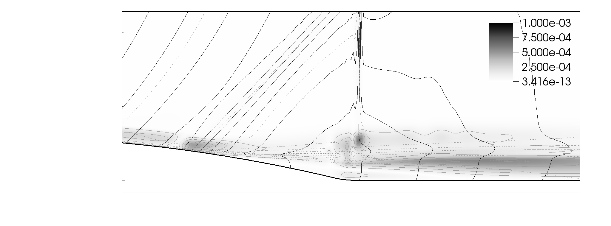
Figure 2: Degree of rarefaction according to Eq. 46 (iso-contours in grayscale) for Délery bump channel flow. 20 pressure isocurves have been added for reference.

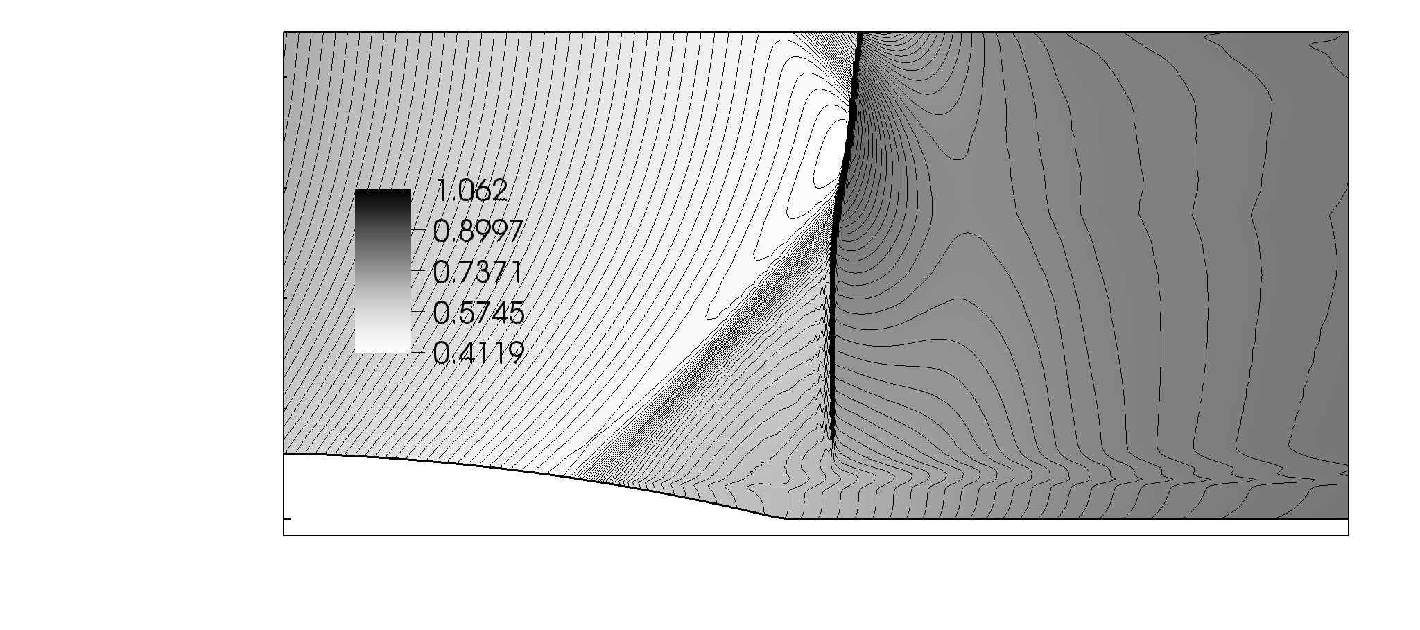
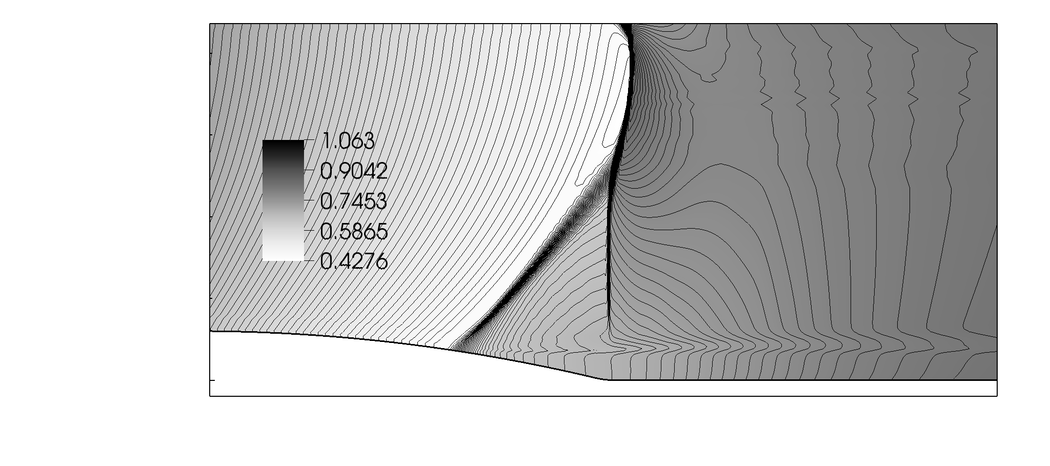
Figure 3: Flow Case 1. Sketches of the shock system in Délery bump channel flow. Gas-kinetic scheme on the left, Navier-Stokes on the right. In both figures, pressure is represented by iso-contours in grayscale. 100 pressure contour lines have also been added.

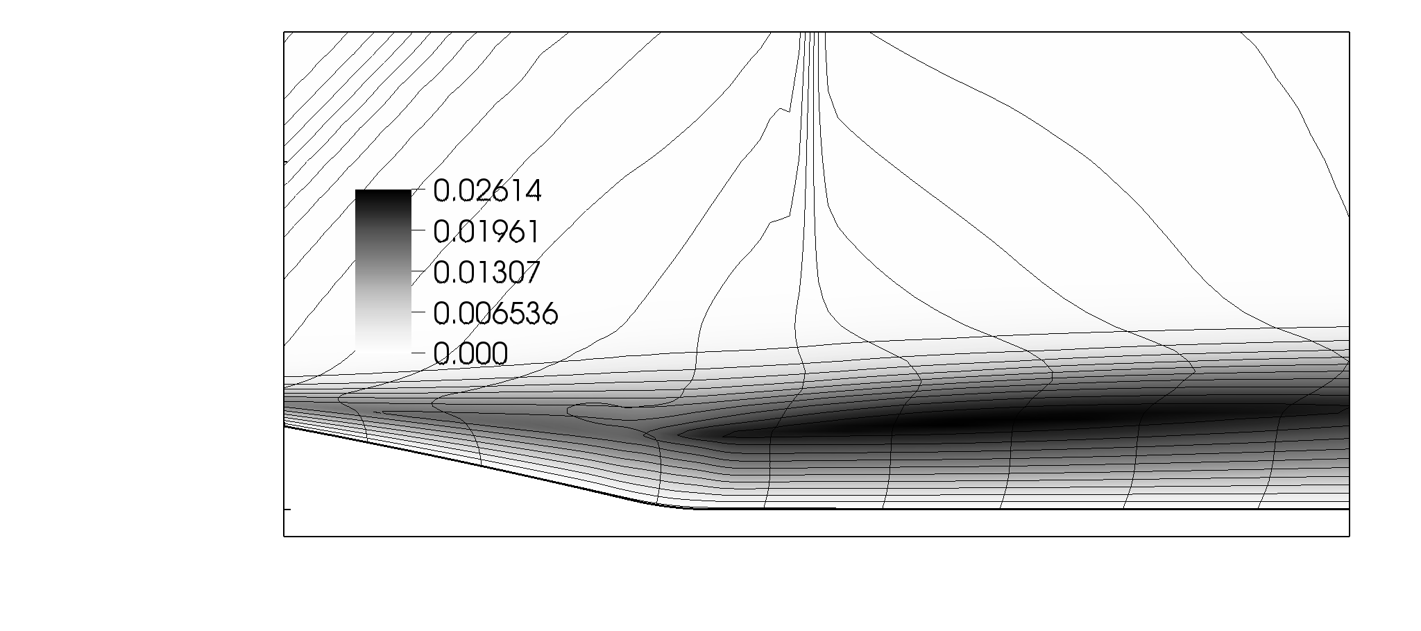
Figure 4: Flow Case 1. Non-dimensional $\tau_{xy}$ component of the turbulent stress tensor in Délery bump channel flow. Experimental values can for instance be found in the measurements by Sartor et al. [25].

3.3.2 Flow Case 2. Supersonic compression corner at high Reynolds number

This flow case concerns the well known experiments carried out by Settles [27]. The experiments include four ramp angles: $8^{\circ}$, $16^{\circ}$, $20^{\circ}$ and $24^{\circ}$. The smallest angle is not sufficient to separate the boundary layer, the $16^{\circ}$ ramp is just enough to cause an incipient separation, whereas separation occurs with the two steeper angles. Whereas conventional schemes seem able to simulate the first two cases (also the computations published by Settles in 1979 [26] were in good agreement with experiments), the separation area is systematically underpredicted.

Pressure and skin friction coefficient obtaind with the turbulent gas-kinetic scheme for Settles’ experiment are shown in Fig. 6. The evidence of grid convergence is shown in Fig. 5 for the $24^{\circ}$ ramp. For all ramp angles, the good agreement in the interaction area is evident whereas the flow after-reattachment is predicted with lower accuracy. A likely cause is related to the inadequacy of the underlying $k$-$\omega$ model to separated flow in supersonic regime.

A further aspect investigated in this flow case is the sensitivity to Reynolds number. In particular, the upstream interaction length has been calculated at different Reynolds numbers (for the $24^{\circ}$ ramp), the results are summarized in Table 2. Interestingly, the lengths calculated seem to fit acceptably into the empirical relation devised by Settles ([9]) for flows at $M\simeq 3$:

$$\left(\frac{L_{0}}{\delta_{0}}\right)\,Re_{\delta_{0}}^{1/3}=0.9e^{0.23\alpha},$$ (50)

where $L_{0}$ is the upstream influence length and $\delta_{0}$ is the boundary layer thickness.

$Re_{\delta_{0}}$	$L_{0}/\delta_{0}$	$\left(\frac{L_{0}}{\delta_{0}}\right)\,Re_{\delta_{0}}^{1/3}$	Error ($\%$)
$740,000$	2.38	216.74	3.53
$1,694,000$	1.98	236.34	5.19
$2,120,000$	1.70	218.15	2.90
$2,912,000$	1.63	233.42	3.90

Table 2: Flow Case 2. Compression corner, $M=2.85$, $\alpha=24^{\circ}$. Sensitivity to Reynolds number. Empirical law $0.9e^{0.23\alpha}$, refer to [9].

Figure 5: Flow Case 2. Grid convergence. (freestream conditions: $M=2.85$, $Re=7.0\times 10^{7}$ per length unit, $\delta_{0}=0.023\,m$). ( ) Gas-kinetic scheme (GKS) on finest grid, (         ) GKS on medium grid (only shown for $\alpha=24^{\circ}$), (             ) GKS on coarsest grid (only shown for $\alpha=24^{\circ}$), (  o  ): experimental data from Settles [26].

Figure 6: Flow Case 2. Pressure and friction coefficient calculated for four different compression corner flows, with angles of $8^{\circ}$, $16^{\circ}$, $20^{\circ}$ and $24^{\circ}$ (freestream conditions: $M=2.85$, $Re=7.0\times 10^{7}$ per length unit, $\delta_{0}=0.023\,m$). ( ) GKS on finest grid, (  o  ): experimental data from Settles [26].

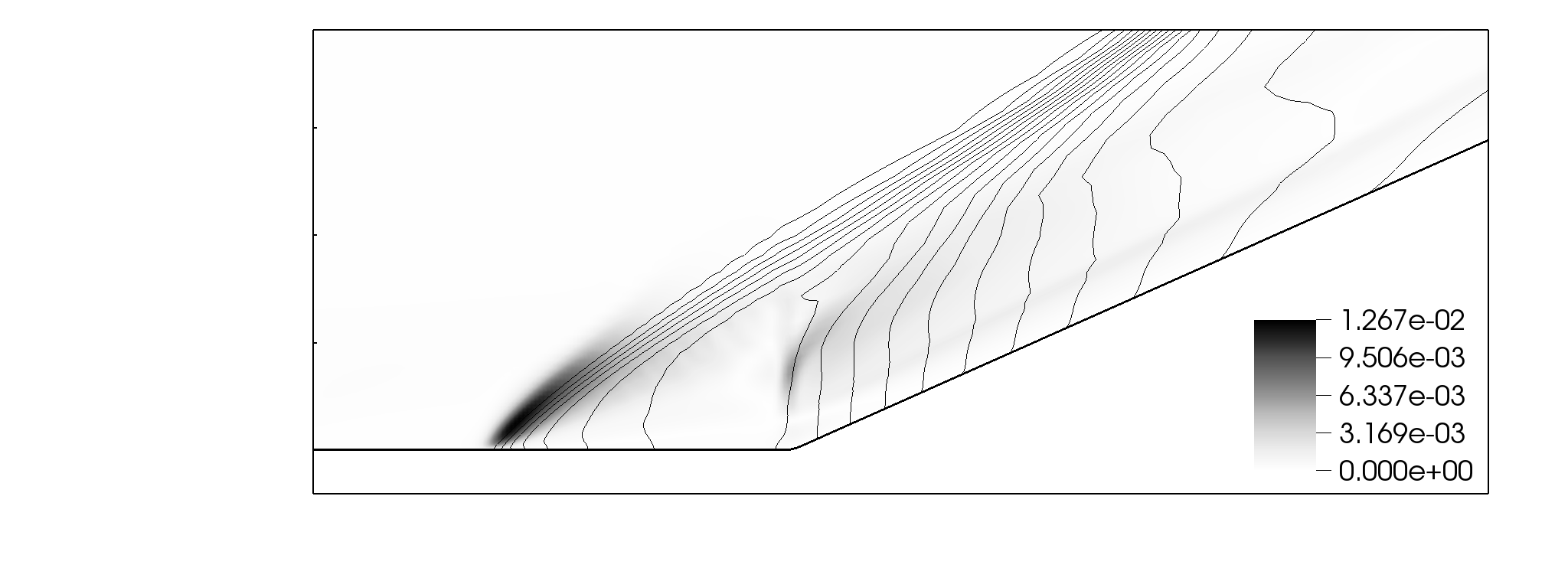
Figure 7: Flow Case 2 $\alpha=24^{\circ}$. Degree of rarefaction according to Eq. 46 in supersonic compression corner flow, $M=2.85$ (iso-contours in grayscale). 20 pressure contour lines have been added for reference.

3.3.3 Flow Cases 3 and 4. Supersonic compression corner and impinging shock at low Reynolds number

Both flow cases refer to the experiments carried out by Bookey [3], devised especially to provide a benchmark case for LES and DNS. The first experiment concerns a ramp with an angle of $24^{\circ}$, the second an impinging shock generated by a ramp with an angle of $12^{\circ}$.

Fig. 8 shows the pressure distributions for both the compression corner and the impinging shock, which are in reasonably good agreement with the experiments. Fig. 9 shows the distribution of the degree of rarefaction in the case of the compression corner, which reaches significant values across the shock wave and on the slip line.

Table 3 summarizes the evaluation of the upstream influence distance - in the case of the compression corner - as a function of Reynolds number, comprised in a range between 1900 and 5000. The trend is compared with Eq. 50, the scaling law proposed by Settles [9] used in Flow Case 2. In particular, the relation between the upstream interaction length and the (displacement thickness based) Reynolds number can be empirically related to Eq. 50 with the exponent changed from $0.23$ to $0.1885$: $\left({L_{0}}/{\delta_{0}}\right)\,Re_{\delta_{0}}^{1/3}=0.9\exp{\left(0.1885\alpha\right)}$.

Figure 8: Flow Cases 3 and 4. Distribution of static pressure calculated for the compression corner (a) with an angle of $24^{\circ}$ and for the reflected shock (b) originating form a compression corner at $12^{\circ}$. Freestream conditions (both flows) are $M=2.90$, $Re_{\theta}=2\;400$. ( ) GKS on grid 1, (             ) GKS on grid 2, (  o  ): experimental data from Bookey [3]. Grid sizes compression corner: $384\times 192$, $512\times 168$ respectively, grid size impinging shock: $384\times 208$, $496\times 304$ respectively. Grid 1 and 2 have different resolution and have been generated with different algorithms.

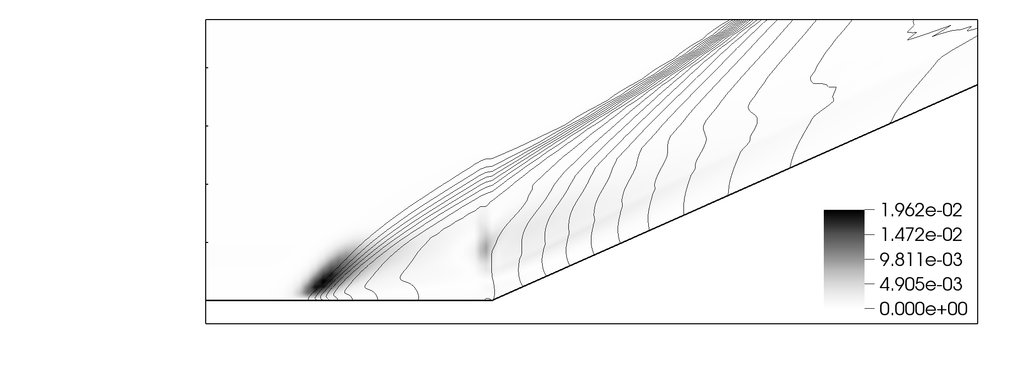
Figure 9: Degree of rarefaction according to Eq. 46 in Flow Case 3, supersonic compression corner, $M=2.90$ (iso-contours in grayscale). 20 pressure contour lines added for reference.

$Re_{\theta}$	$L_{0}/\delta_{0}$	$\left(\frac{L_{0}}{\delta_{0}}\right)\,Re_{\delta_{0}}^{1/3}$	Error ($\%$)
$1\,900$	2.70	80.72	2.03
$2\,300$	2.58	81.85	0.65
$3\,200$	2.35	83.59	1.45
$5\,900$	1.92	84.08	2.05

Table 3: Flow Case 3. Compression corner, $M=2.90$, $\alpha=24^{\circ}$. Upstream influence distance as a function of Reynolds number. Empirical law adjusted to $0.9e^{0.1882\alpha}$ (original: $0.9e^{0.23\alpha}$, refer to [9]).

3.3.4 Flow Case 5. Supersonic impinging shock at low Reynolds number

The experiment by Dupont [11] is similar to flow case 3, carried at a Mach of $2.3$ and a slightly different Reynolds number. It has the advantage of providing results for four different angles: $7^{\circ}$, $8^{\circ}$, $8.8^{\circ}$ and $9.5^{\circ}$ respectively. The pressure distribution is reported in Fig. 10 and shows a reasonably good agreement with the experiment. The degree of rarefaction, shown in Fig. 11, reaches significant values at the foot of the impinging shock and at the separation point.

Figure 10: Flow Case 5. Reflected shock wave at low Reynolds number and Mach $M=2.3$ (experimental data from [11]) with angles ranging from $7.0$ to $9.5$ degrees. $p^{*}=(p-p_{1})/(p_{2}-p_{1})$, where $p_{1}$ and $p_{2}$ are the inviscid pressure values upstream and downstream of shock, respectively. The interaction length $L$ is measured from the foot of the reflected shock to the reattachment point. Results obtained on a grid with size: $496\times 304$.

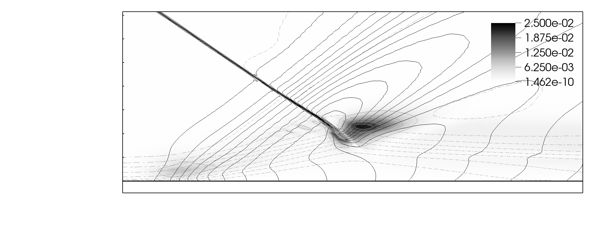
Figure 11: Degree of rarefaction according to Eq. 46 in Flow Case 5, reflected shock, $M=2.30$ (iso-contours in grayscale). 20 pressure contour lines have been added for reference.

3.3.5 Flow Case 6. Supersonic compression corner at Mach $5$

This flow case, investigated by Dolling et al. [10], has been selected to extend the mach Number range to the borders of hypersonics. This flow case has been however calculated assuming adiabatic wall conditions. Results from RANS and hybrid simulations can be found in Edwards et al. [12]. In Fig. 12 the pressure distribution predicted by the turbulent gas-kinetic scheme is compared to the experimental values by Dolling et al. [10], highlighting an acceptable agreement. Fig. 13 shows the distribution of the degree of rarefaction, which reaches values as high as $0.07$.

Figure 12: Compression corner $M=5$, Flow Case 6. Experimental values from Dolling et al. [10]. Results obtained on a grid with size: $384\times 160$

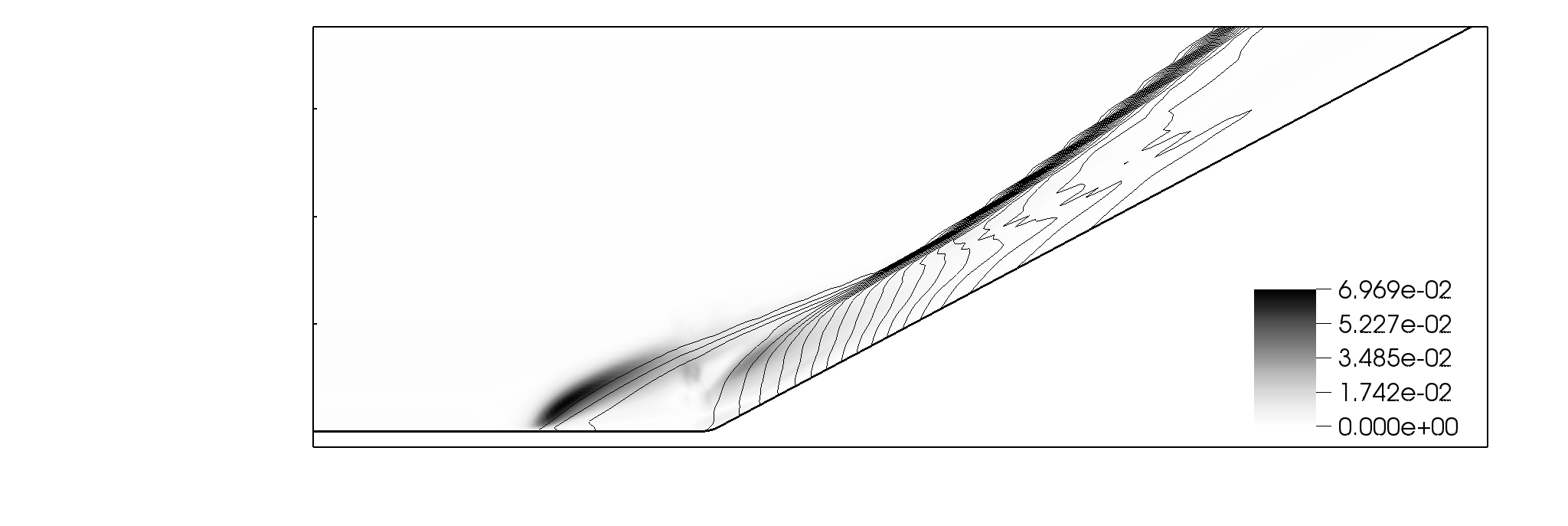
Figure 13: Degree of rarefaction according to Eq. 46 in Flow Case 6, supersonic compression corner, $M=4.95$ (iso-contours in grayscale). 20 pressure contour lines have been added for reference.

4 Conclusions

The predictions obtained with the turbulent gas-kinetic scheme are surprisingly close to the experimental value, at least in terms of mean values and shock position. The turbulent gas-kinetic scheme does not correct in any way the evaluation of the two turbulent quantities, $k$ and $\omega$, provided by the standard model. However, the interaction with the shock is handled, in all examples, in a much more accurate and convincing way. The degree of rarefaction, measured in terms of timescales ratio, reaches in shocklayers values well above the boundary of the continuous regime and definitely in the transitional regime. It is precisely in these “rarefied” flow regions that the gas-kinetic solution differs from the solution obtained with conventional schemes and shows a better agreement with experimental data. Incidentally, rarefaction increases with Mach and decreases with Reynolds. Potentially, the gas-kinetic scheme seems to have the potential to improve predictions in special flow case such as hypersonic flight.

Whereas the turbulent gas-kinetic scheme provides merely a higher accuracy in smooth flow, in the flow regions where the degree of rarefaction reaches significant values, it seems able to deviate from conventional schemes and in so doing provide physically more consistent solutions. The analysis presented in this paper reveals that the turbulent gas-kinetic scheme includes a rarefaction “sensor” which activates the deviations from the conventional schemes. These corrections terms are modeled by the underlying gas kinetic theory and, unlike conventional turbulence modeling, do not require any assumption on the nature of the turbulence nor any series expansion of the turbulent stress tensor.

The properties of turbulent gas-kinetic schemes are still largely unknown. It might be useful to investigate the influence of the main parameters such as order of the Chapman-Enskog expansion for $f_{0}$, reconstruction order, time integration and pre-conditioning. Further, validation is still at its beginnings: three-dimensional flow cases are still unexplored and so is the role played by the choice of the platform model.

An extension to unsteady simulations and in particular to Large Eddy Simulation or to RANS-LES hybrid techniques would be possible without any significant change to the scheme, except for the evaluation of the subgrid turbulent relaxation time. The turbulent gas-kinetic scheme might even be more suitable to LES, since, as pointed out by Chen et al. [6], the largest unresolved scale of motion is normally not much smaller than the smallest resolved scale, leading to large $\tau/\widehat{\tau}$ or $\tau/\Delta t$ ratios.

References

- [1] H. Babinsky and J. K. Harvey. Shock wave-boundary-layer interactions. Cambridge University Press New York, 2011.
- [2] P.L. Bhatnagar, E.P. Gross, and M. Krook. A model for collision processes in gases. I. Small amplitude processes in charged and neutral one-component systems. Phys. Rev., 94(3):511 – 525, 1954.
- [3] P. Bookey, C. Wyckham, and A. Smits. Experimental investigations of Mach 3 shock-wave turbulent boundary layer interactions. AIAA Paper No 2005-4899, 2005.
- [4] C. Cercignani. The Boltzmann equation and its applications. Springer, New York, 1988.
- [5] H. Chen, S. Kandasamy, S. Orszag, R. Shock, S. Succi, and V. Yakhot. Extended Boltzmann kinetic equation for turbulent flows. Science, 301(5633):633–636, 2003.
- [6] H. Chen, S.A. Orszag, I. Staroselsky, and S. Succi. Expanded analogy between Boltzmann kinetic theory of fluids and turbulence. J. Fluid Mech., 519(1):301–314, 2004.
- [7] S.Y. Chou and D. Baganoff. Kinetic flux–vector splitting for the Navier–Stokes equations. J. Comput. Phys., 130(2):217–230, 1997.
- [8] J. Délery. Experimental investigation of turbulence properties in transonic shock/boundary-layer interactions. AIAA J., 21:180–185, 1983.
- [9] J. Délery, J.G. Marvin, and E Reshotko. Shock-wave boundary layer interactions. AGARDograph, 280, 1986.
- [10] D. S. Dolling and M. E Erengil. Unsteady wave structure near separation in a Mach 5 compression rampinteraction. AIAA J, 29(5):728–735, 1991.
- [11] P Dupont, C Haddad, and JF Debiève. Space and time organization in a shock-induced separated boundary layer. J. Fluid Mech., 559:255–278, 2006.
- [12] J. R. Edwards. Numerical simulations of shock/boundary layer interactions using time-dependent modeling techniques: A survey of recent results. Prog. Aerosp. Sci., 44(6):447–465, 2008.
- [13] E. Garnier, N. Adams, and P. Sagaut. Large eddy simulation for compressible flows. Springer, 2009.
- [14] U. Goldberg, O. Peroomian, and S. Chakravarthy. Application of the k-e-R Turbulence Model to Wall-Bounded Compressive Flows. AIAA Paper No. 98-0323, (Paper No. 98-0323), 1998.
- [15] A. Jameson. Solution of the Euler equations for two dimensional transonic flow by a multigrid method. Appl. Math. Comput., 13(3-4):327–356, 1983.
- [16] M. N Kogan. Rarefied gas dynamics. Plenum Press, New York, 1969.
- [17] Q. Li, K. Xu, and S. Fu. A high-order gas-kinetic Navier–Stokes flow solver. Journal of Computational Physics, 229(19):6715–6731, 2010.
- [18] W. Liao, L. Luo, and K. Xu. Gas-kinetic scheme for continuum and near-continuum hypersonic flows. J. Spacecraft Rockets, 44(6):1232–1240, 2007.
- [19] J.C. Mandal and S.M. Deshpande. Kinetic flux vector splitting for Euler equations. Comput. Fluids, 23(2):447–478, 1994.
- [20] G. May, B. Srinivasan, and A. Jameson. An improved gas-kinetic BGK finite-volume method for three-dimensional transonic flow. J. Comput. Phys., 220(2):856–878, 2007.
- [21] S. Pirozzoli, M. Bernardini, and F. Grasso. Direct numerical simulation of transonic shock/boundary layer interaction under conditions of incipient separation. J. Fluid Mech., 657:361–393, 2010.
- [22] S.B. Pope. Turbulent flows. Cambridge Univ. Pr., Cambridge, 2000.
- [23] M. Righi. A Gas-Kinetic Scheme For The Simulation Of Turbulent Flows. In M. Mareschal and A. Santos, editors, Proceeding of the 28th Internaltional Symposium on Rarefied Gas Dynamics, Zaragoza, pages 481–488. American Institute of Physics, 2012.
- [24] M. Righi. A finite-volume gas-kinetic method for the solution of the Navier-Stokes equations. Royal Aeronautical Society, Aeronaut. J., (117)(1192), 2013.
- [25] F. Sartor, G. Losfeld, and R. Bur. Piv study on a shock-induced separation in a transonic flow. Exp. Fluids, 53(3):815–827, 2012.
- [26] G.S. Settles, T.J. Fitzpatrick, and S.M. Bogdonoff. Detailed study of attached and separated compression corner flowfields in high Reynolds number supersonic flow. AIAA J., 17(6):579–585, 1979.
- [27] G.S. Settles, I.E. Vas, and S.M. Bogdonoff. Details of a shock-separated turbulent boundary layer at a compression corner. AIAA J., 14(12):1709–1715, 1976.
- [28] S Succi, O Filippova, H Chen, and S Orszag. Towards a renormalized lattice boltzmann equation for fluid turbulence. J. Stat. Phyis., 107(1-2):261–278, 2002.
- [29] S. Wallin and A.V. Johansson. An explicit algebraic Reynolds stress model for incompressible and compressible turbulent flows. J. Fluid Mech., 403:89–132, 2000.
- [30] D. C. Wilcox. Turbulence Modeling for CFD, 3rd edition. DCW Industries, Inc., La Canada CA, 2006.
- [31] K. Xu. Gas-kinetic schemes for unsteady compressible flow simulations. Von Karman Institute, Computational Fluid Dynamics, Annual Lecture Series, 29th, Rhode-Saint-Genese, Belgium, 1998.
- [32] K. Xu. A gas-kinetic BGK scheme for the Navier–Stokes equations and its connection with artificial dissipation and Godunov method. J. Comput. Phys., 171(1):289–335, 2001.
- [33] K. Xu and J. Huang. A unified gas-kinetic scheme for continuum and rarefied flows. J. Comput. Phys., 229(20):7747–7764, 2010.
- [34] K. Xu, M. Mao, and L. Tang. A multidimensional gas-kinetic BGK scheme for hypersonic viscous flow. J. Comput. Phys., 203(2):405–421, 2005.
- [35] K. Xu and K.H. Prendergast. Numerical Navier-Stokes solutions from gas kinetic theory. J. Comput. Phys., 114(1):9–17, 1994.
- [36] L. Xuan and K. Xu. A new gas-kinetic scheme based on analytical solutions of the bgk equation. J. of Comput. Phys., 2012.
- [37] S. Yoon and A. Jameson. Lower-upper symmetric-Gauss-Seidel method for the Euler and Navier-Stokes equations. AIAA J., 26(9):1025–1026, 1988.