Steady-State Entanglement in the Nuclear Spin Dynamics of a Double Quantum Dot

Abstract

We propose a scheme for the deterministic generation of steady-state entanglement between the two nuclear spin ensembles in an electrically defined double quantum dot. Due to quantum interference in the collective coupling to the electronic degrees of freedom, the nuclear system is actively driven into a two-mode squeezed-like target state. The entanglement build-up is accompanied by a self-polarization of the nuclear spins towards large Overhauser field gradients. Moreover, the feedback between the electronic and nuclear dynamics leads to multi-stability and criticality in the steady-state solutions.

Entanglement is a key ingredient to applications in quantum information science. In practice, however, it is very fragile and is often destroyed by the undesired coupling of the system to its environment, hence robust ways to prepare entangled states are called for. Schemes that exploit open system dynamics to prepare them as steady states are particularly promising kraus04 ; verstraete09 ; diehl08 ; muschik11 ; sanchez13 . Here, we investigate such a scheme in quantum information architectures using spin qubits in quantum dots awschalom02 ; hanson07 . In these systems, a great deal of research has been directed towards the complex interplay between electron and nuclear spins rudner11a ; rudner11b ; schuetz12 ; ono04 ; vink09 ; gullans10 ; chekhovich13 ; danon09 , with the ultimate goal of turning the nuclear spins from the dominant source of decoherence johnson05 ; koppens05 ; khaetskii02 ; bluhm10 into a useful resource foletti09 ; taylor03 ; witzel07 ; ribeiro10 . The creation of entanglement between nuclear spins constitutes a pivotal element towards these goals.

In this work, we propose a scheme for the dissipative preparation of steady-state entanglement between the two nuclear spin ensembles in a double quantum dot (DQD) in the Pauli-blockade regime ono02 ; hanson07 . The entanglement arises from an interference between different hyperfine-induced processes lifting the Pauli-blockade. This becomes possible by suitably engineering the effective electronic environment, which ensures a collective coupling of electrons and nuclei (i.e., each flip can happen either in the left or the right QD and no which-way information is leaked), and that just two such processes with a common entangled stationary state are dominant. Engineering of the electronic system via external gate voltages facilitates the control of the desired steady-state properties. Exploiting the separation of electronic and nuclear time-scales allows to derive a quantum master equation in which the interference effect becomes apparent: It features non-local jump operators which drive the nuclear system into an entangled steady state of EPR-type muschik11 . Since the entanglement is actively stabilized by the dissipative dynamics, our approach is inherently robust against weak random perturbations kraus04 ; verstraete09 ; diehl08 ; muschik11 ; sanchez13 . The entanglement build-up is accompanied by a self-polarization of the nuclear system towards large Overhauser (OH) field gradients if a small initial gradient is provided. Upon surpassing a certain threshold value of this field the nuclear dynamics turn self-polarizing, and drive the system to even larger gradients. Entanglement is then generated in the quantum fluctuations around these macroscopic nuclear polarizations. Furthermore, feedback between electronic and nuclear dynamics leads to multi-stability and criticality in the steady-state solutions.

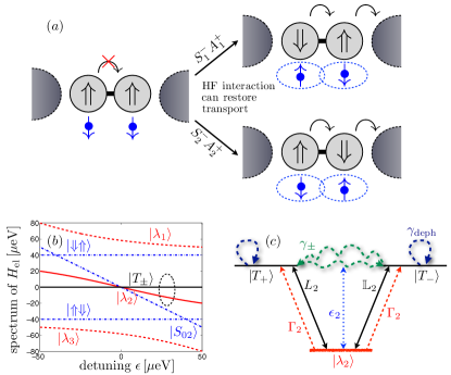
Figure 1: (color online). (a) Schematic illustration of nuclear entanglement generation via electron transport. Whenever the Pauli-blockade is lifted via the HF interaction with the nuclear spins, a nuclear flip can occur in either of the two dots. The local nature of the HF interaction is masked by the non-local character of the electronic level $\left|\lambda_{2}\right\rangle$. (b) Spectrum of $H_{\mathrm{el}}$ for $\Delta=40\mu\mathrm{eV}$ and $t=30\mu\mathrm{eV}$. The three eigenstates $\left|\lambda_{k}\right\rangle$ are displayed in red. The triplets $\left|T_{\pm}\right\rangle$ are degenerate for $\omega_{0}=0$. In this setting, lifting of the spin blockade due to HF interaction is pre-dominantly mediated by the non-local jump operators required for two-mode squeezing, namely $L_{2}$ and $\mathbb{L}_{2}$. The ellipse refers to a potential operational area of our scheme. (c) The resulting effective three-level system $\left\{\left|T_{\pm}\right\rangle,\left|\lambda_{2}\right\rangle\right\}$ including coherent HF coupling and the relevant dissipative processes: $\left|\lambda_{2}\right\rangle$ decays according to its overlap with $\left|S_{02}\right\rangle$ with an effective decay rate $\Gamma_{2}=\left|\left<\lambda_{2}|S_{02}\right>\right|^{2}\Gamma$ Gamma . Within this three-level subspace, purely electronic Pauli-blockade lifting mechanisms like cotunneling or spin-orbital effects result in effective dephasing and dissipative mixing rates, labeled as $\gamma_{\mathrm{deph}}$ and $\gamma_{\pm}$, respectively.

We consider a DQD in the Pauli-blockade regime ono02 ; hanson07 ; see Fig. 1. A source-drain bias across the device induces electron transport via the cycle $\left(0,1\right)\rightarrow\left(1,1\right)\rightarrow\left(0,2\right)\rightarrow\left(0,1\right)$. Here, $\left(m,n\right)$ refers to a configuration with $m\left(n\right)$ electrons in the left (right) dot, respectively. The only energetically accessible $(0,2)$ state is the localized singlet, $\left|S_{02}\right\rangle$. Then, by the Pauli principle, the interdot charge transition $\left(1,1\right)\rightarrow\left(0,2\right)$ is allowed only for the $(1,1)$ spin-singlet $\left|S_{11}\right\rangle=\left(\left|\Uparrow\Downarrow\right\rangle-\left|\Downarrow\Uparrow\right\rangle\right)/\sqrt{2}$, while the spin-triplet states $\left|T_{\pm}\right\rangle$ and $\left|T_{0}\right\rangle=\left(\left|\Uparrow\Downarrow\right\rangle+\left|\Downarrow\Uparrow\right\rangle\right)/\sqrt{2}$ are blocked. Including a homogeneous Zeeman splitting $\omega_{0}$ and a magnetic gradient $\Delta$, both oriented along $\hat{z}$, the DQD within the relevant two-electron subspace is then described by the effective Hamiltonian $\left(\hbar=1\right)$

$$H_{\mathrm{el}} = \omega_{0}\left(S_{1}^{z}+S_{2}^{z}\right)+\Delta\left(S_{2}^{z}-S_{1}^{z}\right)-\epsilon\left|S_{02}\right\rangle\left\langle S_{02}\right|$$ (1)

$$+t\left(\left|\Uparrow\Downarrow\right\rangle\left\langle S_{02}\right|-\left|\Downarrow\Uparrow\right\rangle\left\langle S_{02}\right|+\mathrm{h.c.}\right),$$

where $\epsilon$ refers to the relative interdot energy detuning between the left and right dot and $t$ describes interdot electron tunneling in the Pauli-blockade regime.

The spin blockade inherent to $H_{\mathrm{el}}$ can be lifted, e.g., by the hyperfine (HF) interaction with nuclear spins in the host environment. The electronic spins $\vec{S}_{i}$ confined in either of the two dots $\left(i=1,2\right)$ are coupled to two different sets of nuclei $\left\{\sigma_{i,j}^{\alpha}\right\}$ via the isotropic Fermi contact interaction schliemann03

$$H_{\mathrm{HF}}=\frac{a_{\mathrm{hf}}}{2}\sum_{i=1,2}\left(S_{i}^{+}A_{i}^{-}+S_{i}^{-}A_{i}^{+}\right)+a_{\mathrm{hf}}\sum_{i=1,2}S_{i}^{z}A_{i}^{z}.$$ (2)

Here, $S_{i}^{\alpha}$ and $A_{i}^{\alpha}=\sum_{j}a_{i,j}\sigma_{i,j}^{\alpha}$ for $\alpha=\pm,z$ denote electron and collective nuclear spin operators, and $a_{i,j}$ defines the unitless HF coupling constant between the electron spin in dot $i$ and the $j$th nucleus: $\sum_{j=1}^{N_{i}}a_{i,j}=N$, where $N=\left(N_{1}+N_{2}\right)/2\sim 10^{6}$ refers to the average number of nuclei per dot. The individual nuclear spin operators $\sigma_{i,j}^{\alpha}$ are assumed to be spin-$\frac{1}{2}$ and we neglect the nuclear Zeeman and dipole-dipole terms schliemann03 . The second term in Eq.(2) can be split into an effective nuclear magnetic field and residual quantum fluctuations, $H_{\mathrm{zz}}=a_{\mathrm{hf}}\sum_{i=1,2}S_{i}^{z}\delta A_{i}^{z}$, where $\delta A_{i}^{z}=A_{i}^{z}-\left\langle A_{i}^{z}\right\rangle_{t}$. The (time-dependent) semiclassical OH field exhibits a homogeneous $\bar{\omega}_{\text{$\mathrm{OH}$}}=\frac{a_{\mathrm{hf}}}{2}\left(\left\langle A_{1}^{z}\right\rangle_{t}+\left\langle A_{2}^{z}\right\rangle_{t}\right)$ and inhomogeneous component $\Delta_{\text{$\mathrm{OH}$}}=\frac{a_{\mathrm{hf}}}{2}\left(\left\langle A_{2}^{z}\right\rangle_{t}-\left\langle A_{1}^{z}\right\rangle_{t}\right)$, which can be absorbed into the definitions of $\omega_{0}$ and $\Delta$ in Eq.(1) as $\omega_{0}=\bar{\omega}_{\text{$\mathrm{OH}$}}+\omega_{\mathrm{ext}}$ and $\Delta=\Delta_{\text{$\mathrm{OH}$}}+\Delta_{\mathrm{ext}}$, respectively. For now, we assume the symmetric situation of vanishing external fields $\omega_{\mathrm{ext}}=\Delta_{\mathrm{ext}}=0$ SuppInfo . Thus, $\omega_{0}$ and $\Delta$ are dynamic variables depending on the nuclear polarizations.

The flip-flop dynamics, given by the first term in Eq. (2) and the OH fluctuations described by $H_{\mathrm{zz}}$ can be treated perturbatively with respect to the effective electronic Hamiltonian $H_{\mathrm{el}}$. Its eigenstates within the $S_{\mathrm{tot}}^{z}=S_{1}^{z}+S_{2}^{z}=0$ subspace can be expressed as $\left|\lambda_{k}\right\rangle=\mu_{k}\left|\Uparrow\Downarrow\right\rangle+\nu_{k}\left|\Downarrow\Uparrow\right\rangle+\kappa_{k}\left|S_{02}\right\rangle$ ($k=1,2,3$) with corresponding eigenenergies $\epsilon_{k}$. For $t\gg\omega_{0},g_{\mathrm{hf}}$, where $g_{\mathrm{hf}}=\sqrt{N}a_{\text{hf}}$, $\left|\lambda_{1,3}\right\rangle$ are far detuned, and the electronic subsystem can be simplified to an effective three-level system comprising the levels $\left\{\left|T_{\pm}\right\rangle,\left|\lambda_{2}\right\rangle\right\}$. Effects arising due to the presence of $\left|\lambda_{1,3}\right\rangle$ will be discussed below. Within this reduced scheme, $H_{\mathrm{ff}}$ reads

$$H_{\mathrm{ff}}=\frac{a_{\mathrm{hf}}}{2}\left[L_{2}\left|\lambda_{2}\right\rangle\left\langle T_{+}\right|+\mathbb{L}_{2}\left|\lambda_{2}\right\rangle\left\langle T_{-}\right|+\mathrm{h.c.}\right],$$ (3)

where the non-local nuclear operators $L_{2}=\nu_{2}A_{1}^{+}+\mu_{2}A_{2}^{+}$ and $\mathbb{L}_{2}=\mu_{2}A_{1}^{-}+\nu_{2}A_{2}^{-}$ are associated with lifting the Pauli-blockade from $\left|T_{+}\right\rangle$ and $\left|T_{-}\right\rangle$ via $\left|\lambda_{2}\right\rangle$, respectively. They can be controlled via the external parameters $t$ and $\epsilon$ defining the amplitudes $\mu_{2}$ and $\nu_{2}$.

The dynamical evolution of the system is described in terms of a Markovian master equation for the reduced density matrix of the DQD system $\rho$ describing the relevant electronic and nuclear degrees of freedom schuetz12 . Besides the HF dynamics described above, it accounts for other purely electronic mechanisms like, e.g., cotunneling. These effects and their implications for the nuclear dynamics are described in SuppInfo and lead to effective decay and dephasing processes in the $T_{\pm}$ subspace with rates $\gamma_{\pm},\gamma_{\mathrm{deph}}$; see Fig. 1 (c). For fast electronic dynamics ($\gamma_{\pm},\gamma_{\mathrm{deph}}\gg g_{\mathrm{hf}}$) and a sufficiently high gradient $\Delta\gtrsim 3\mu\mathrm{eV}$ (see SuppInfo ), the hybridized electronic level $\left|\lambda_{2}\right\rangle$ exhibits a significant overlap with the localized singlet $\left|S_{02}\right\rangle$ and the electronic subsystem settles in the desired quasi-steady state, $\rho_{\mathrm{ss}}^{\mathrm{el}}=\left(\left|T_{+}\right\rangle\left\langle T_{+}\right|+\left|T_{-}\right\rangle\left\langle T_{-}\right|\right)/2$, on a time-scale much shorter than the nuclear dynamics. One can then adiabatically eliminate all electronic coordinates yielding a coarse-grained equation of motion for the nuclear density matrix $\sigma=\mathsf{Tr}_{\mathrm{el}}\left[\rho\right]$, where $\mathsf{Tr}_{\mathrm{el}}\left[\dots\right]$ denotes the trace over the electronic degrees of freedom: $\dot{\sigma}=\mathcal{L}_{\mathrm{id}}\left[\sigma\right]+\mathcal{L}_{\mathrm{nid}}\left[\sigma\right]$. Here, the first dominant term describes the desired nuclear squeezing dynamics

$$\mathcal{L}_{\mathrm{id}}\left[\sigma\right] = \frac{\gamma}{2}\left[\mathcal{D}\left[L_{2}\right]\sigma+\mathcal{D}\left[\mathbb{L}_{2}\right]\sigma\right]$$ (4)

$$+i\frac{\delta}{2}\left(\left[L_{2}^{\dagger}L_{2},\sigma\right]+\left[\mathbb{L}_{2}^{\dagger}\mathbb{L}_{2},\sigma\right]\right),$$

where $\mathcal{D}\left[c\right]\rho=c\rho c^{\dagger}-\frac{1}{2}\left\{c^{\dagger}c,\rho\right\}$. It arises from coupling to the level $\left|\lambda_{2}\right\rangle$, while $\mathcal{L}_{\mathrm{nid}}\left[\sigma\right]$ results from coupling to the far detuned levels $\left|\lambda_{1,3}\right\rangle$ and OH fluctuations described by $H_{\mathrm{zz}}$ SuppInfo . Here, $\gamma$ and $\delta$ refer to a HF-mediated decay rate and Stark shift, respectively .

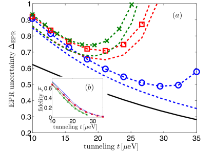
Figure 2: (color online). Steady-state entanglement between the two nuclear spin ensembles quantified via (a) the EPR-uncertainty $\Delta_{\mathrm{EPR}}$ and (b) fidelity $\mathcal{F}$ of the nuclear steady state with the two-mode squeezed target state. The black solid curve refers to the idealized setting where the undesired HF coupling to $\left|\lambda_{1,3}\right>$ has been ignored and where $J_{1}=J_{2}=pJ_{\mathrm{max}}$, $p=0.8$ and $N_{1}=N_{2}=2J_{\mathrm{max}}=10^{6}$, corresponding to $\Delta_{\mathrm{OH}}=40\mu\mathrm{eV}$. The blue-dashed line then also takes into account coupling to $\left|\lambda_{1,3}\right>$ while the red-dashed curve in addition accounts for an asymmetric dot size: $N_{2}=0.8N_{1}=8\times 10^{5}$. The amount of entanglement decreases for a smaller nuclear polarization: $p=0.7$ (green dashed curve). Classical uncertainty (symbols) in the total spin $J_{i}$ quantum numbers leads to less entanglement, but does not destroy it. Here, we have set the range of the distribution to $\Delta_{J_{i}}=50\sqrt{N_{i}}$. Other numerical parameters: $\omega_{0}=0$, $\Gamma=25\mu\mathrm{eV}$, $\epsilon=30\mu\mathrm{eV}$ and $\gamma_{\pm}+\gamma_{\mathrm{deph}}/2=1\text{$\mu$}\mathrm{eV}$.

Pure stationary solutions $\left|\xi_{\mathrm{ss}}\right\rangle$ associated with the dynamics generated by Eq.(4) can be obtained from the dark-state condition $L_{2}\left|\xi_{\mathrm{ss}}\right\rangle=\mathbb{L}_{2}\left|\xi_{\mathrm{ss}}\right\rangle=0$. First, we consider the limit of equal dot sizes $(N_{1}=N_{2})$ and uniform HF coupling $\left(a_{i,j}=N/N_{i}\right)$, and generalize our results later. The nuclear system can be described via Dicke states $\left|J_{i},k_{i}\right\rangle$, where $k_{i}=0,1,\dots,2J_{i}$ and $J_{i}$ refer to the spin-$\hat{z}$ projection and total spin quantum numbers, respectively. For $J_{1}=J_{2}=J$, one readily checks that the dark-state condition is satisfied by the (unnormalized) pure state $\left|\xi_{\mathrm{ss}}\right\rangle=\sum_{k=0}^{2J}\xi^{k}\left|J,k\right\rangle\otimes\left|J,2J-k\right\rangle$, representing an entangled state closely similar to the two-mode squeezed state SuppInfo . The parameter $\xi=-\nu_{2}/\mu_{2}$ quantifies the entanglement and polarization of the nuclear system. $\left|\xi\right|<1$ ($\left|\xi\right|>1$) corresponds to states of large positive (negative) OH gradients, respectively. The system is invariant under the symmetry transformation ($\mu_{2}\leftrightarrow\nu_{2}$, $A_{1,2}^{z}\rightarrow-A_{1,2}^{z}$) which gives rise to a bistability in the steady state, as for every solution with positive OH gradient ($\Delta>0$), we find another one with $\Delta<0$.

For a given $\left|\xi\right|\neq 1$ the individual nuclear polarizations in the state $\left|\xi_{\mathrm{ss}}\right\rangle$ approach one as we increase the system size $J$, and we can describe the system dynamics in the vicinity of the respective steady state in the framework of a Holstein-Primakoff (HP) transformation kessler12 . This allows for a detailed analysis of the nuclear dynamics including perturbative effects from the processes described by $\mathcal{L}_{\text{nid}}$. The collective nuclear spins $I_{i}^{\alpha}=\sum_{j}\sigma_{i,j}^{\alpha}$ are mapped to bosonic operators and the (unique) ideal steady state is well-known to be a two-mode squeezed state muschik11 ; SuppInfo which represents $\left|\xi_{\mathrm{ss}}\right\rangle$ within the HP picture. Since in the bosonic case the modulus of $\xi$ is confined to $|\xi|<1$, the HP analysis refers to one of the two symmetric steady-state solutions mentioned above. Within the HP approximation the dynamics generated by $\dot{\sigma}=\mathcal{L}_{\mathrm{id}}\left[\sigma\right]+\mathcal{L}_{\mathrm{nid}}\left[\sigma\right]$ are quadratic in the new bosonic creation and annihilation operators. Therefore, the nuclear dynamics are purely Gaussian and exactly solvable. The generation of entanglement can be certified via the EPR entanglement condition muschik11 ; raymer03 , $\Delta_{\mathrm{EPR}}<1$, where $\Delta_{\mathrm{EPR}}=\left[\mathrm{var}\left(I_{1}^{x}+I_{2}^{x}\right)+\mathrm{var}\left(I_{1}^{y}+I_{2}^{y}\right)\right]/\left(\left|\left<I_{1}^{z}\right>\right|+\left|\left<I_{2}^{z}\right>\right|\right)$. While $\Delta_{\mathrm{EPR}}\geq 1$ for separable states, the ideal dynamics $\mathcal{L}_{\mathrm{id}}$ drive the nuclear spins into an EPR state with $\Delta_{\mathrm{EPR}}^{\mathrm{id}}=\left(1-\left|\xi\right|\right)/\left(1+\left|\xi\right|\right)<1$. As illustrated in Fig. 2, we numerically find that the generation of steady-state entanglement persists even for asymmetric dot sizes of $\sim 20\%$, classical uncertainty in the total spins $J_{i}$ and the undesired terms $\mathcal{L}_{\mathrm{nid}}$. When tuning $t$ from $10\mu\mathrm{eV}$ to $35\mu\mathrm{eV}$, the squeezing parameter $|\xi|$ increases from $\sim 0.2$ to $\sim 0.6$, respectively. For $|\xi|\approx 0.2$, we obtain a relatively high fidelity $\mathcal{F}$ with the ideal two-mode squeezed state, close to 80$\%$. For stronger squeezing, the target state becomes more susceptible to the undesired noise terms, first leading to a reduction of $\mathcal{F}$ and eventually to a break-down of the HP approximation. The associated critical behavior can be understood in terms of a dissipative phase transition kessler12 ; schuetz13 .

We now turn to the experimental realization of our scheme SuppInfo : In the analysis above, we discussed the idealized case of uniform HF coupling. However, our scheme also works for non-uniform coupling, provided that the two dots are sufficiently similar: If the coupling is completely inhomogeneous, that is $a_{i,j}\neq a_{i,k}$ for all $j\neq k$, but the two QDs are identical $\left(a_{1,j}=a_{2,j}\forall j=1,\dots,N_{1}\equiv N_{2}\right)$, Eq.(4) supports a unique pure entangled stationary state. Up to normalization, it reads $\left|\xi_{\mathrm{ss}}\right\rangle=\otimes_{j=1}^{N}\left|\xi\right\rangle_{j}$, where $\left|\xi\right\rangle_{j}=\left|\downarrow_{j},\uparrow_{j}\right\rangle+\xi\left|\uparrow_{j},\downarrow_{j}\right\rangle$ is an entangled state of two nuclear spins belonging to different nuclear ensembles . $\left|\xi_{\mathrm{ss}}\right>$ features a (large) polarization gradient $\Delta_{I^{z}}=\left\langle I_{2}^{z}\right\rangle-\left\langle I_{1}^{z}\right\rangle=N\frac{1-\xi^{2}}{1+\xi^{2}}$.

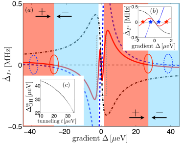
Figure 3: (color online). Semiclassical solution to the nuclear polarization dynamics. (a) Instantaneous nuclear polarization rate $\dot{\Delta}_{I^{z}}$ as a function of the gradient $\Delta$ for $t=20\mu\mathrm{eV}$ (blue dashed), $t=30\mu\mathrm{eV}$ (red solid) and $t=50\mu\mathrm{eV}$ (black dash-dotted). FPs are found at $\dot{\Delta}_{I^{z}}=0$. The ovals mark stable high-gradient steady state solutions. The background coloring refers to the sign of $\dot{\Delta}_{I^{z}}$ (for $t=30\mu\mathrm{eV}$) which determines the stable FP the nuclear system is attracted to (see arrows). (b) Zoom-in of (a) into the low-gradient regime: The unpolarized FP lies at $\Delta=0$, whereas critical, instable points $\Delta_{\mathrm{OH}}^{\mathrm{crt}}$ (marked by stars) can be identified with $\dot{\Delta}_{I^{z}}=0$ and $d\dot{\Delta}_{I^{z}}/d\Delta>0$. (c) Stable high-polarization FPs $\Delta_{\mathrm{OH}}^{\mathrm{ss}}$ (see ovals) as a function of $t$; for $t\approx 10\mu\mathrm{eV}$ we obtain a nuclear polarization of $\sim 90\%$. Other numerical parameters: $\Gamma=25\mu\mathrm{eV}$, $\epsilon=30\mu\mathrm{eV}$, $\gamma_{\pm}=0.3\text{$\mu$}\mathrm{eV}$ and $\gamma_{\mathrm{deph}}=0.5\text{$\mu$}\mathrm{eV}$.

The build-up of a large OH gradient is corroborated within a semiclassical calculation which neglects correlations among the nuclear spins SuppInfo . This is valid on time scales long compared to nuclear dephasing mechanisms gullans10 ; christ07 . Assuming equal dot sizes, $N_{1}=N_{2}=N$, we use a semiclassical factorization scheme christ07 resulting in decoupled equations of motion for the two nuclear polarization variables $\left\langle I_{1}^{z}\right\rangle_{t}$ and $\left\langle I_{2}^{z}\right\rangle_{t}$ . In particular, $\Delta_{I^{z}}$ evolves as

$$\frac{d}{dt}\Delta_{I^{z}} = -\gamma_{\mathrm{eff}}\left[\Delta_{I^{z}}-N\frac{\chi}{\gamma_{\mathrm{eff}}}\right],$$ (5)

where the HF-mediated depolarization $\gamma_{\mathrm{eff}}$ and pumping rate $\chi$ (see SuppInfo for their connection to microscopic parameters) depend on the gradient $\Delta$ defined in Eq. (1), in particular on the OH gradient $\Delta_{\mathrm{OH}}\propto\Delta_{I^{z}}$. The electron-nuclear feedback-loop can then be closed self-consistently by identifying steady-state solutions of Eq. (5) in which the parameter $\Delta$ is provided by the nuclear OH gradient only. The instantaneous polarization rate $\dot{\Delta}_{I^{z}}$, given in Eq. (5), is displayed in Fig. 3 as a function of $\Delta$, with the electronic subsystem in its respective steady state, yielding a non-linear equation for the nuclear equilibrium polarizations. Stable fixed points (FPs) are determined by $\dot{\Delta}_{I^{z}}=0$ and $d\dot{\Delta}_{I^{z}}/d\Delta<0$ as opposed to instable ones where $d\dot{\Delta}_{I^{z}}/d\Delta>0$ vink09 ; danon09 ; bluhm10b . We can identify parameter regimes in which the nuclear system features three FPs which are interspersed by two instable points. Two of the stable FPs are high-polarization solutions of opposite sign, supporting a macroscopic OH gradient, while one is the trivial, zero polarization solution. If the initial gradient lies outside the instable points, the system turns self-polarizing and the OH gradient approaches a highly polarized FP. For typical parameter values we estimate that the OH gradient at the instable points is $\approx(1-2)\mu\mathrm{eV}$; compare Fig. 3 (b). This comparatively moderate initial gradient could be achieved via, e.g., a nanomagnet pioro08 ; petersen13 or alternative dynamic nuclear polarization schemes foletti09 ; gullans10 ; petta08 ; takahashi11 .

Next, we address the effects of weak nuclear interactions: First, we have neglected nuclear dipole-dipole interactions. However, we estimate the time scale for the entanglement creation as $t^{*}=\hbar/N\gamma\lesssim 10\mu\mathrm{s}$ which is fast compared to typical nuclear decoherence times, recently measured to be $\sim 1\mathrm{ms}$ in vertical DQDs takahashi11 . Thus, it should be possible to create entanglement between the two nuclear spin ensembles faster than it gets disrupted by dipole-dipole interactions among the nuclei. Second, we have disregarded nuclear Zeeman terms since our scheme requires no external homogeneous magnetic field for sufficiently strong tunneling $t$ .

Finally, entanglement could be detected by measuring the OH shift in each dot separately hanson07 ; in combination with NMR techniques to rotate the nuclear spins chekhovich13 we can obtain all spin components and their variances which are sufficient to verify the presence of entanglement (similar to the proposal rudner11a ).

To conclude, we have presented a scheme for the dissipative entanglement generation among the two nuclear spin ensembles in a DQD. This may provide a long-lived, solid-state entanglement resource and a new route for nuclear-spin-based information storage and manipulation.

Acknowledgments.—We acknowledge support by the DFG within SFB 631, the Cluster of Excellence NIM and the project MALICIA within the 7th Framework Programme for Research of the European Commission, under FET-Open grant number: 265522. EMK acknowledges support by the Harvard Quantum Optics Center and the Institute for Theoretical Atomic and Molecular Physics. LV acknowledges support by the Dutch Foundation for Fundamental Research on Matter (FOM).

Appendix A Supplementary Information (SI)

The following supplementary information (SI) provides additional background material to specific topics of the main text. First, we discuss the master equation used to model the dynamics of the DQD. Then, by eliminating all electronic coherences, we derive an effective description for the nuclear dynamics. Thereafter, it is shown that this description can be simplified substantially in the high gradient regime where the electronic level $\left|\lambda_{2}\right>$ can be eliminated from the dynamics. The explicit form of the noise terms labeled by $\mathcal{L}_{\mathrm{nid}}$ in the main text is given thereafter. The following section presents analytical and numerical results on the ideal nuclear target state, for both uniform and non-uniform HF coupling. Next, we present details on the Holstein-Primakoff mapping and give the so-called standard form of the covariance matrix which has been used for the evaluation of the EPR uncertainty $\Delta_{\mathrm{EPR}}$ within the HP approximation. Finally, we provide some details regarding our semiclassical approach to study the nuclear self-polarization effects, discuss the effect of external magnetic fields and summarize the requirements for an experimental realization of our scheme.

Contents

1. A Supplementary Information (SI)
   1. A.1 The Model
   2. A.2 Effective Nuclear Dynamics
   3. A.3 High Gradient Regime
   4. A.4 Noise Terms
   5. A.5 Hyperfine Coupling and Ideal Nuclear Steady State
   6. A.6 Holstein-Primakoff Transformation
   7. A.7 EPR Uncertainty
   8. A.8 Polarization Dynamics
   9. A.9 External Magnetic Fields
   10. A.10 Summary of Experimental Requirements

A.1 The Model

After tracing out the unobserved degrees of freedom of the leads, the dynamical evolution of the system can be described in terms of an effective Markovian master equation for the reduced density matrix of the DQD system $\rho$ describing the relevant electronic as well as the nuclear subsystem. Within the relevant three-level subspace $\{\left|T_{\pm}\right\rangle,\left|\lambda_{2}\right\rangle\}$, it reads

$$\dot{\rho} = \mathcal{L}_{0}\left[\rho\right]+\mathcal{V}\left[\rho\right]$$ (6)

$$\mathcal{L}_{0}\left[\rho\right] = -i\left[H_{\mathrm{el}},\rho\right]+\Gamma_{2}\sum_{\nu=\pm}\mathcal{D}\left[\left|T_{\nu}\right\rangle\left\langle\lambda_{2}\right|\right]\rho$$

$$+\gamma_{\pm}\sum_{\nu=\pm}\mathcal{D}\left[\left|T_{\bar{\nu}}\right\rangle\left\langle T_{\nu}\right|\right]\rho+\mathcal{L}_{\mathrm{deph}}\left[\rho\right],$$

where $\mathcal{V}\left[\rho\right]=-i\left[H_{\mathrm{ff}}+H_{\mathrm{zz}},\rho\right]$ and $\mathcal{D}\left[c\right]\rho$ is a short-hand notation for the Lindblad term $\mathcal{D}\left[c\right]\rho=c\rho c^{\dagger}-\frac{1}{2}\left\{c^{\dagger}c,\rho\right\}$. In deriving Eq.(6), we have neglected terms rotating at a frequency of $\epsilon_{l}-\epsilon_{k}$ for $k\neq l$ and dissipative terms acting entirely within the fast subspace, i.e., terms of the form $\mathcal{D}\left[\left|\lambda_{k}\right\rangle\left\langle\lambda_{j}\right|\right]$; for typical parameters, we have checked that the simplified Liouvillian given in Eq.(6) reproduces exactly the electronic quasi steady state (fulfilling $\mathcal{L}_{0}\left[\rho_{\mathrm{ss}}^{\mathrm{el}}\right]=0$). Moreover, it describes very well the electronic asymptotic decay rate, that is the spectral gap of $\mathcal{L}_{0}$, which quantifies the long-time behavior of the electronic subsystem kessler12 ; schuetz13 and is therefore relevant for a good description of the nuclear dynamics.

Electron transport.—Apart from the unitary dynamics discussed in the main text, Eq.(6) contains three dissipative terms: The first one, proportional to $\Gamma_{2}=\left|\left<\lambda_{2}|S_{02}\right>\right|^{2}\Gamma$, describes electron transport as the hybridized level $\left|\lambda_{2}\right\rangle$ acquires a finite lifetime according to its overlap with the localized singlet $\left|S_{02}\right\rangle$. Here, $\Gamma$ is given by

$$\Gamma=\Gamma_{R}/2,$$ (7)

where

$$\Gamma_{\alpha}=2\pi|T_{\alpha}|^{2}n_{\alpha},$$ (8)

denotes the typical sequential tunneling rate to the lead $\alpha=L,R$; the tunnel matrix element $T_{\alpha}$ specifies the transfer coupling between the lead $\alpha$ and the DQD system and $n_{\alpha}$ refers to the density of states per spin in the lead $\alpha$ schuetz12 . By making the left tunnel barrier more transparent than the right one $(2\Gamma_{L}\gg\Gamma_{R})$, we can eliminate the intermediate stage in the sequential tunneling process $\left(0,2\right)\rightarrow\left(0,1\right)\rightarrow\left(1,1\right)$ petersen13 ; schuetz12 . Then, on relevant time scales, the DQD is always in the two-electron regime and electron transport is fully described by the effective rate $\Gamma$.

Other mechanisms.—The second and third dissipative term account for decay processes from $\left|T_{+}\right\rangle$ to $\left|T_{-}\right\rangle$ and vice versa and dephasing between the triplets $\left|T_{\pm}\right\rangle$ which is modeled by the Lindblad term

$$\mathcal{L}_{\mathrm{deph}}\left[\rho\right]=\frac{\gamma_{\mathrm{deph}}}{2}\mathcal{D}\left[\left|T_{+}\right\rangle\left\langle T_{+}\right|-\left|T_{-}\right\rangle\left\langle T_{-}\right|\right]\rho.$$ (9)

For the sake of theoretical generality, this is a common phenomenological description for distinct physical mechanisms like e.g. cotunneling, spin-exchange with the leads or spin-orbital effects which may also lift the Pauli blockade and therefore contribute to electron transport through the DQD device, but, in contrast to the HF interaction, do so without affecting the nuclear spins directly. In accordance with a typical experimental situation, they are weak compared to direct tunneling in the singlet subspace, but may still be fast compared to the typical HF time scale $g_{\mathrm{hf}}=A_{\mathrm{HF}}/\sqrt{N}\approx 0.1\mu\mathrm{eV}$.

Our regime of interest can be summarized as

$$1\gg\gamma_{\pm}/\Gamma,\gamma_{\mathrm{deph}}/\Gamma\gg g_{\mathrm{hf}}/\Gamma.$$ (10)

The right hand side can be suppressed efficiently by working in a regime of strong electron exchange with the leads. For typical values, we estimate $g_{\mathrm{hf}}/\Gamma\approx(2-4)\times 10^{-3}$. In particular, this condition allows us to adiabatically eliminate all electronic coherences for $\gamma_{\pm}+\gamma_{\mathrm{deph}}/2\gg g_{\mathrm{hf}}$ and, in the high gradient regime specified below, all electronic coordinates can be eliminated for $2\gamma_{\pm}\gg g_{\mathrm{hf}}$.

Cotunneling.—For example, let us briefly show how virtual tunneling processes via localized triplet states fit into this effective, phenomenological description. Usually, they are neglected because they are far off in energy due to the relatively large singlet-triplet splitting $\Delta_{\mathrm{st}}\gtrsim 400\mu\mathrm{eV}$ hanson07 . Still, they may contribute to electron transport by lifting the spin blockade as follows: The triplet $\left|T_{\pm}\right\rangle$ with $\left(1,1\right)$ charge configuration is coherently coupled to the localized triplet $\left|T_{\pm}\left(0,2\right)\right\rangle$ by the interdot tunneling coupling $t$. This transition is strongly detuned by the singlet-triplet splitting $\Delta_{\mathrm{st}}$. Once, the energetically high lying level $\left|T_{\pm}\left(0,2\right)\right\rangle$ is populated, it quickly decays with an effective rate $\Gamma$ either back to $\left|T_{\pm}\right\rangle$ giving rise to pure dephasing or to $\left|T_{\mp}\right\rangle$ via some fast intermediate steps. The former contributes to $\gamma_{\mathrm{deph}}$, while the latter can be absorbed into the phenomenological rate $\gamma_{\pm}$. Using standard second order perturbation theory, the effective rate for this mechanism can be estimated as

$$\gamma_{\mathrm{ct}}/\Gamma=x_{\mathrm{ct}}\approx\left(\frac{t}{\Delta_{\mathrm{st}}}\right)^{2}.$$ (11)

Compared to direct electronic processes, it is lowered by the ’penalty’ factor $x_{\mathrm{ct}}$, which we estimate as $x_{\mathrm{ct}}\approx(30/400)^{2}\approx 0.005$.

Spin-orbit.—Other mechanisms besides cotunneling also contribute to the phenomenological rates $\gamma_{\mathrm{deph}}$ and $\gamma_{\pm}$. For example, along the lines of the cotunneling analysis, spin-orbital effects can be accounted for. The corresponding penalty factor can be estimated as

$$x_{\mathrm{so}}\approx\frac{t_{\mathrm{so}}^{2}}{\epsilon^{2}+\Gamma^{2}},$$ (12)

where the spin-orbit coupling parameter is approximately $t_{\mathrm{so}}\approx(0.01-0.1)t$ schreiber11 ; giavaras13 . This gives the order-of-magnitude estimate $x_{\mathrm{so}}\approx 3^{2}/(30^{2}+25^{2})\approx 0.006$.

On a similar footing, one can also account for spin-exchange with the leads schuetz13 . The different electronic decay channels have to be summed up as $\gamma_{\pm}=\gamma_{\mathrm{ct}}+\gamma_{\mathrm{so}}+\dots$ and $\gamma_{\mathrm{deph}}=\gamma_{\mathrm{ct}}+\gamma_{\mathrm{so}}+\dots$. Based on the estimates stated above, sufficiently strong electron exchange with the leads ensures the validity of Eq.(10).

A.2 Effective Nuclear Dynamics

In the limit $\gamma_{\text{$\pm$}}+\gamma_{\mathrm{deph}}/2\gg g_{\mathrm{hf}}$, any electronic coherences decay rapidly on typical nuclear time scales. Using standard techniques, we can then adiabatically eliminate them from the dynamics yielding a simplified coarse-grained equation of motion for the nuclear density matrix $\sigma=\mathsf{Tr}_{\mathrm{el}}\left[\rho\right]$, where $\mathsf{Tr}_{\mathrm{el}}\left[\dots\right]$ denotes the trace over the electronic degrees of freedom. Since differences in the populations of the triplets $\left|T_{+}\right>$ and $\left|T_{-}\right>$ are quickly damped to zero with a rate of $2\gamma_{\pm}$, it is approximately given by

$$\dot{\sigma} = \gamma\left\{p_{+}\left[\mathcal{D}\left[L_{2}\right]\sigma+\mathcal{D}\left[\mathbb{L}_{2}\right]\sigma\right]\right.$$

$$\left.+\left(1-2p_{+}\right)\left[\mathcal{D}\left[L_{2}^{\dagger}\right]\sigma+\mathcal{D}\left[\mathbb{L}_{2}^{\dagger}\right]\sigma\right]\right\}$$

$$+i\delta\left\{p_{+}\left(\left[L_{2}^{\dagger}L_{2},\sigma\right]+\left[\mathbb{L}_{2}^{\dagger}\mathbb{L}_{2},\sigma\right]\right)\right.$$

$$\left.-\left(1-2p_{+}\right)\left(\left[L_{2}L_{2}^{\dagger},\sigma\right]+\left[\mathbb{L}_{2}\mathbb{L}_{2}^{\dagger},\sigma\right]\right)\right\},$$

where $\gamma$ and $\delta$ refer to the effective rate

$$\gamma=\frac{a_{\mathrm{hf}}^{2}\tilde{\Gamma}}{2[\tilde{\Gamma}^{2}+\epsilon_{2}^{2}]}$$ (14)

and Stark shift

$$\delta=(\epsilon_{2}/2\tilde{\Gamma})\gamma,$$ (15)

respectively. Here, we have set $\tilde{\Gamma}=\Gamma_{2}+\gamma_{\pm}/2+\gamma_{\mathrm{deph}}/4$. The nuclear dynamics are governed by the non-local jump operators $L_{2}$ and $\mathbb{L}_{2}$, describing HF-mediated nuclear flips from $\left|T_{+}\right\rangle$ and $\left|T_{-}\right\rangle$ to $\left|\lambda_{2}\right\rangle$, respectively, but still coupled to the electronic subsystem via the population of the triplet $\left|T_{+}\right\rangle$, $p_{+}$. On a coarse-grained time scale relevant for the nuclear dynamics, all electronic coherences are fully depleted and the populations (given by $p_{+}$, $p_{-}=p_{+}$ and $p_{2}=1-2p_{+}$, respectively) completely characterize the electronic subsystem. Therefore, the coupled electron-nuclear DQD system is described by Eq.(A.2), complemented by an equation of motion for $p_{+}$, which, in turn, depends on the state of the nuclear spins schuetz13 . In Eq.(A.2) we have suppressed contributions arising from the OH fluctuations, governed by $H_{\mathrm{zz}}$. This is in line with the semiclassical approximation to study the nuclear polarization dynamics. However, as stated in the main text, they have been taken into account when analyzing the steady state entanglement properties of the nuclear system (see below).

A.3 High Gradient Regime

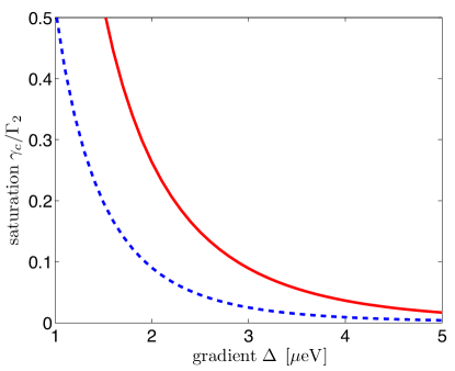
Figure 4: (color online). Saturation parameter $\gamma_{c}/\Gamma_{2}$ as a function of the gradient $\Delta$ for $t=20\mu\mathrm{eV}$ (blue dashed) and $t=30\mu\mathrm{eV}$ (red solid), respectively. In the high gradient regime, where this value is sufficiently low, the electronic level $\left|\lambda_{2}\right\rangle$ can be eliminated adiabatically from the dynamics as it gets fully depleted on relevant nuclear time scales. Other numerical parameters are: $\Gamma=25\mu\mathrm{eV}$, $\epsilon=30\mu\mathrm{eV}$, $\gamma_{\mathrm{deph}}=0.5\mu\mathrm{eV}$ and $\gamma_{\pm}=0.3\mu\mathrm{eV}$.

For a sufficiently high gradient $\Delta$, the electronic level $\left|\lambda_{2}\right\rangle$ exhibits a significant overlap with the localized singlet $\left|S_{02}\right\rangle$; accordingly, in this regime the electronic degrees of freedom can be eliminated completely from the dynamics. More rigorously, this holds for

$$\frac{\gamma_{c}}{\Gamma_{2}}=\frac{g_{\mathrm{hf}}^{2}}{2\left[\tilde{\Gamma}^{2}+\epsilon_{2}^{2}\right]}\frac{\tilde{\Gamma}}{\Gamma_{2}}\ll 1,$$ (16)

where $\gamma_{c}=N\gamma$ comprises a factor of $N\approx 10^{6}$ to account for typical HF-mediated interaction strengths of $g_{\mathrm{hf}}=\sqrt{N}a_{\mathrm{hf}}\approx 0.1\mu\mathrm{eV}$. As shown in Fig. 4, for typical parameters $\left|\lambda_{2}\right\rangle$ can be eliminated adiabatically for $\Delta\gtrsim\left(2-3\right)\mu\mathrm{eV}$. In this regime, the electronic subsystem settles to a quasi steady-state, given by $\rho_{\mathrm{ss}}^{\mathrm{el}}=\left(\left|T_{+}\right\rangle\left\langle T_{+}\right|+\left|T_{-}\right\rangle\left\langle T_{-}\right|\right)/2$, on a time scale much shorter than the nuclear dynamics. The effective nuclear dynamics in the submanifold of this electronic quasi steady state $\rho_{\mathrm{ss}}^{\mathrm{el}}$ gives rise to the Liouvillian stated in the main text in Eq.(4).

A.4 Noise Terms

For completeness, here we present the explicit form of the superoperator $\mathcal{L}_{\mathrm{nid}}\left[\sigma\right]$ which can be decomposed as

$$\mathcal{L}_{\mathrm{nid}}\left[\sigma\right]=\mathcal{K}_{\mathrm{fz}}\left[\sigma\right]+\mathcal{K}^{\mathrm{nid}}_{\mathrm{ff}}\left[\sigma\right]+\mathcal{K}_{\mathrm{zz}}\left[\sigma\right].$$ (17)

The first term is given by

$$\mathcal{K}_{\mathrm{fz}}\left[\sigma\right] = -i\frac{a_{\mathrm{hf}}}{2}\sum_{i,\alpha=\pm}\left\langle S_{i}^{\alpha}\right\rangle_{\mathrm{ss}}\left[A_{i}^{\bar{\alpha}},\sigma\right]$$ (18)

$$-ia_{\mathrm{hf}}\sum_{i}\left\langle S_{i}^{z}\right\rangle_{\mathrm{ss}}\left[\delta A_{i}^{z},\sigma\right].$$

Here, $\left\langle\cdot\right\rangle_{\mathrm{ss}}=\mathsf{Tr}_{\mathrm{el}}\left[\cdot\rho_{\mathrm{ss}}^{\mathrm{el}}\right]$ denotes the steady state expectation value. Next, undesired, second-order HF-mediated transitions to the electronic levels $\left|\lambda_{1,3}\right>$ are described by

$$\mathcal{K}^{\mathrm{nid}}_{\mathrm{ff}}\left[\sigma\right] = \sum_{k\neq 2}\left[\frac{\gamma_{k}}{2}\mathcal{D}\left[L_{k}\right]\sigma+i\frac{\delta_{k}}{2}\left[L_{k}^{\dagger}L_{k},\sigma\right]\right.$$ (19)

$$\left.+\frac{\gamma_{k}}{2}\mathcal{D}\left[\mathbb{L}_{k}\right]\sigma+i\frac{\delta_{k}}{2}\left[\mathbb{L}_{k}^{\dagger}\mathbb{L}_{k},\sigma\right]\right],$$

where we have introduced the generalized, effective HF-mediated decay rates

$$\gamma_{k} = \frac{a_{\mathrm{hf}}^{2}\tilde{\Gamma}_{k}}{2\left[\epsilon_{k}^{2}+\tilde{\Gamma}_{k}^{2}\right]},$$ (20)

with the dephasing rate $\tilde{\Gamma}_{k}=\Gamma_{k}+\gamma_{\mathrm{\pm}}/2+\gamma_{\mathrm{deph}}/4$, the transport-mediated level width of $\left|\lambda_{k}\right>$ being $\Gamma_{k}=\kappa_{k}^{2}\Gamma$ and the nuclear Stark shifts

$$\delta_{k} = \frac{a_{\mathrm{hf}}^{2}\epsilon_{k}}{4\left[\epsilon_{k}^{2}+\tilde{\Gamma}_{k}^{2}\right]}.$$ (21)

The non-local nuclear operators $L_{k}$ and $\mathbb{L}_{k}$ are defined as $L_{k}=\nu_{k}A_{1}^{+}+\mu_{k}A_{2}^{+}$ and $\mathbb{L}_{k}=\mu_{k}A_{1}^{-}+\nu_{k}A_{2}^{-}$, respectively. Finally, the last term reads

$$\mathcal{K}_{\mathrm{zz}}\left[\sigma\right]=\gamma_{\mathrm{zz}}\sum_{i,j}\left[\delta A_{j}^{z}\sigma\delta A_{i}^{z}-\frac{1}{2}\left\{\delta A_{i}^{z}\delta A_{j}^{z},\sigma\right\}\right],$$ (22)

where $\gamma_{\mathrm{zz}}=a_{\mathrm{hf}}^{2}/4\gamma_{\pm}$.

A.5 Hyperfine Coupling and Ideal Nuclear Steady State

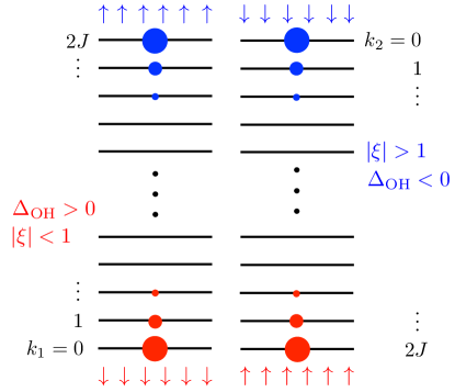
Figure 5: (color online). Sketch of the ideal nuclear dark state for uniform HF coupling $\left|\xi_{\mathrm{ss}}\right\rangle$. The Dicke states are labeled according to their spin projection $k_{i}=0,1,\dots 2J$. Since $k_{1}=k$ is strongly correlated with $k_{2}=2J-k$, the two Dicke ladders are arranged in opposite order. The bistability inherent to $\left|\xi_{\mathrm{ss}}\right\rangle$ is schematized as well: The size of the spheres refers to $\left|\left<k_{1},k_{2}|\xi_{\mathrm{ss}}\right>\right|^{2}$ for $\left|\xi\right|<1$ (red) and $\left|\xi\right|>1$ (blue), respectively. As indicated by the arrows for individual nuclear spins, $\left|\xi\right|<1$ $\left(\left|\xi\right|>1\right)$ corresponds to a nuclear OH gradient $\Delta_{\mathrm{OH}}>0$ $\left(\Delta_{\mathrm{OH}}>0\right)$, respectively.

In the main text, the HP analysis has been performed for uniform hyperfine coupling. This simplification is based on the assumption that the electron density is approximately constant in the dots and zero outside rudner11a . In Ref.schwager10 , it was shown that corrections to this idealized setting are of the order of $1-p$ for high polarization $p$. Therefore, the analysis for uniform HF coupling is correct to zeroth order in the small parameter $1-p$. To make connection with a realistic situation, the underlying idea is to express the HF coupling constants as $a_{i,j}=\bar{a}+\delta_{i,j}$, where the dominant uniform term $\bar{a}$ enables an efficient description within fixed $J_{i}$ subspaces, while the non-uniform contribution $\delta_{i,j}$ leads to a coupling between different $J_{i}$ subspaces on a much longer time scale. The latter is relevant in order to reach highly polarized nuclear states christ07 .

We have explicitly stated the ideal nuclear steady state $\left|\xi_{\mathrm{ss}}\right>$, fulfilling $L_{2}\left|\xi_{\mathrm{ss}}\right>=\mathbb{L}_{2}\left|\xi_{\mathrm{ss}}\right>=0$, for two ’opposing’ limits: First, we analytically construct the ideal (pure) nuclear steady-state in the limit of identical dots $(a_{1j}=a_{2j}\forall j=1,\dots,N_{1}\equiv N_{2}=N)$ for uniform HF-coupling where $a_{ij}=N/N_{i}$. In this limit, the non-local nuclear jump operators simplify to

$$L_{2} = \nu I_{1}^{+}+\mu I_{2}^{+},$$ (23)

$$\mathbb{L}_{2} = \mu I_{1}^{-}+\nu I_{2}^{-}.$$ (24)

Here, to simplify the notation, we have replaced $\mu_{2}$ and $\nu_{2}$ by $\mu$ and $\nu$, respectively. The common proportionality factor is irrelevant for this analysis and therefore has been dropped. The collective nuclear spin operators $I_{1,2}^{\alpha}$ form a spin algebra and the so-called Dicke states $\left|J_{1},k_{1}\right\rangle\otimes\left|J_{2},k_{2}\right\rangle\equiv\left|J_{1},k_{1};J_{2},k_{2}\right\rangle$, where the total spin quantum numbers $J_{i}$ are conserved and the spin projection quantum number $k_{i}=0,1,\dots,2J_{i}$, allow for an efficient description. Here, we restrict ourselves to the symmetric case where $J_{1}=J_{2}=J$; analytic and numerical evidence for small $J_{i}\approx 3$ shows, that for $J_{1}\neq J_{2}$ one obtains a mixed nuclear steady state schuetz13 . The total spin quantum numbers $J_{i}=J$ are conserved and we set $\left|J,k_{1};J,k_{2}\right\rangle=\left|k_{1},k_{2}\right\rangle$. Using standard angular momentum relations, one obtains

$$L_{2}\left|k_{1},k_{2}\right\rangle = \nu j_{k_{1}}\left|k_{1}+1,k_{2}\right\rangle+\mu j_{k_{2}}\left|k_{1},k_{2}+1\right\rangle,$$ (25)

$$\mathbb{L}_{2}\left|k_{1},k_{2}\right\rangle = \mu g_{k_{1}}\left|k_{1}-1,k_{2}\right\rangle+\nu g_{k_{2}}\left|k_{1},k_{2}-1\right\rangle.$$ (26)

Here, we have introduced the matrix elements

$$j_{k} = \sqrt{J\left(J+1\right)-\left(k-J\right)\left(k-J+1\right)},$$ (27)

$$g_{k} = \sqrt{J\left(J+1\right)-\left(k-J\right)\left(k-J-1\right)}.$$ (28)

Note that $j_{2J}=0$ and $g_{0}=0$. Moreover, the matrix elements obey the symmetry

$$j_{k} = j_{2J-k-1},$$ (29)

$$g_{k+1} = g_{2J-k}.$$ (30)

Now, we show that $\left|\xi_{\mathrm{ss}}\right\rangle$ fulfills $L_{2}\left|\xi_{\mathrm{ss}}\right\rangle=\mathbb{L}_{2}\left|\xi_{\mathrm{ss}}\right\rangle=0$. First, using the relations above, we have

$$L_{2}\left|\xi_{\mathrm{ss}}\right\rangle = \sum_{k=0}^{2J}\xi^{k}\left[\nu j_{k}\left|k+1,2J-k\right\rangle\right.$$

$$\left.+\mu j_{2J-k}\left|k,2J-k+1\right\rangle\right]$$

$$= \sum_{k=0}^{2J-1}\xi^{k}\left[\nu j_{k}\left|k+1,2J-k\right\rangle\right.$$

$$\left.+\xi\mu j_{2J-k-1}\left|k+1,2J-k\right\rangle\right]$$

$$= \sum_{k=0}^{2J-1}\xi^{k}\nu\underset{=0}{\underbrace{\left[j_{k}-j_{2J-k-1}\right]}}\left|k+1,2J-k\right\rangle.$$

In the second step, since $j_{2J}=0$, we have redefined the summation index as $k\rightarrow k+1$. Along the same lines, one obtains

$$\mathbb{L}_{2}\left|\xi_{\mathrm{ss}}\right\rangle = \sum_{k=0}^{2J}\xi^{k}\left[\mu g_{k}\left|k-1,2J-k\right\rangle\right.$$

$$\left.+\nu g_{2J-k}\left|k,2J-k-1\right\rangle\right]$$

$$= \sum_{k=0}^{2J-1}\xi^{k}\left[\xi\mu g_{k+1}\left|k,2J-k-1\right\rangle\right.$$

$$\left.+\nu g_{2J-k}\left|k,2J-k-1\right\rangle\right]$$

$$= \sum_{k=0}^{2J-1}\xi^{k}\nu\underset{=0}{\underbrace{\left[g_{2J-k}-g_{k+1}\right]}}\left|k,2J-k-1\right\rangle.$$

This completes the proof. For illustration, the dark state $\left|\xi_{\mathrm{ss}}\right\rangle$ is sketched in Fig. 5. In particular, the bistable polarization character inherent to $\left|\xi_{\mathrm{ss}}\right\rangle$ is emphasized, as (in contrast to the bosonic case) the modulus of the parameter $\xi$ is not confined to $\left|\xi\right|<1$.

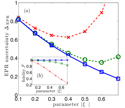
Figure 6: (color online). EPR uncertainty $\Delta_{\mathrm{EPR}}$ (a) and fidelity $\mathcal{F}$ with the nuclear target state $\left|\xi_{\mathrm{ss}}\right>$ (b) as a function of the squeezing parameter $\left|\xi\right|$ for $N_{1}=N_{2}=3$ inhomogeneously coupled nuclear spins. The blue curve (squares) refers to an symmetric setting where $\vec{a}_{1}=\vec{a}_{2}=\left(1.11,1.67,0.22\right)$, whereas the green (circles) and red (crosses) curves incorporate asymmetries: $\vec{a}_{1}=\left(1.18,1.61,0.21\right)$, $\vec{a}_{2}=\left(1.11,1.67,0.22\right)$ and $\vec{a}_{1}=\left(1,1.5,0.5\right)$, $\vec{a}_{2}=\left(1.24,1.55,0.21\right)$, respectively.

Second, we have elaborated on the case of a perfectly inhomogeneous distribution of HF coupling constants. For identical QDs, the nuclear spins can always be grouped into pairs $\left(a_{1,j}=a_{2,j}\right)$. In the absence of degeneracies, i.e., for $a_{i,j}\neq a_{i,k}$ for all $j\neq k$, we have identified the nuclear dark state as $\left|\xi_{\mathrm{ss}}\right\rangle=\otimes_{j=1}^{N}\left|\xi\right\rangle_{j}$. This analytical result is verified by exact diagonalization for small systems of inhomogeneously coupled nuclear spins $\left(N_{1}=N_{2}=3\right)$: see Fig. 6. It indicates that $\left|\xi_{\mathrm{ss}}\right\rangle$ is the unique steady state. Moreover, as long as the squeezing parameter is $\left|\xi\right|\lesssim 0.5$, the nuclear system is found to be robust against asymmetries $\left(\vec{a}_{1}\neq\vec{a}_{2}\right)$ and features entanglement over a broad range of the parameter $\left|\xi\right|$.

Note that one can ’continuously’ go from the case of non-degenerate HF coupling constants to the limit of uniform HF coupling by grouping spins with the same HF coupling constants to ’shells’, which form collective nuclear spins. For degenerate couplings, however, there are additional conserved quantities and therefore multiple stationary states of the above form. If $a_{1,j}\approx a_{2,j}$ we expect (and have also verified for small $N$, see Fig. 6) that the resulting mixed stationary state is still unique (in the non-degenerate case) and close to $\left|\xi_{\mathrm{ss}}\right\rangle$.

A.6 Holstein-Primakoff Transformation

The (exact) Holstein-Primakoff transformation expresses the truncation of the collective nuclear spin operators to a total spin $J_{i}$ subspace in terms of a bosonic mode kessler12 . For $\Delta>0\left(\left|\xi\right|<1\right)$ the nuclear ensembles are polarized in opposite directions, and the (zeroth order) HP mapping for the collective nuclear spins $I_{i}^{\alpha}=\sum_{j}\sigma_{i,j}^{\alpha}$ $(\alpha=\pm,z)$ reads explicitly

$$I_{1}^{-} \approx \sqrt{2J_{1}}b_{1},$$ (31)

$$I_{1}^{z} = b_{1}^{\dagger}b_{1}-J_{1}.$$ (32)

for the first nuclear ensemble, and similarly for the second ensemble

$$I_{2}^{+} \approx \sqrt{2J_{2}}b_{2},$$ (33)

$$I_{1}^{z} = J_{2}-b_{2}^{\dagger}b_{2}.$$ (34)

We consider the subspace with large collective spin quantum numbers, that is $J_{i}\sim\mathcal{O}\left(N/2\right)$. Thus, the zeroth-order HP mapping given above can be justified self-consistently, provided that the occupations in the bosonic modes $b_{i}$ are small compared to $2J_{i}$ kessler12 .

For equal dot sizes and $J_{1}=J_{2}=J$, the nuclear jump operators are mapped to $L_{2}\sim a$ and $\mathbb{L}_{2}\sim\tilde{a}$, where $a=\mu b_{2}+\nu b_{1}^{\dagger}$ and $\tilde{a}=\mu b_{1}+\nu b_{2}^{\dagger}$. Here, we have set $\mu=\mu_{2}/\sqrt{\mu_{2}^{2}-\nu_{2}^{2}}$ and similarly for $\nu$ such that $\mu^{2}-\nu^{2}=1$. In this picture, the (unique) ideal steady state is well-known to be a two-mode squeezed state

$$\left|\Psi_{\mathrm{TMS}}\right\rangle=\mu^{-1}\sum_{n}\xi^{n}\left|n,n\right\rangle,$$ (35)

which is simply the vacuum in the non-local bosonic modes $a$ and $\tilde{a}$ fulfilling $a\left|\Psi_{\mathrm{TMS}}\right\rangle=\tilde{a}\left|\Psi_{\mathrm{TMS}}\right\rangle=0$ muschik11 .

The generation of entanglement can be certified via the EPR entanglement condition muschik11 ; raymer03 , where the EPR-uncertainty is given by

$$\Delta_{\mathrm{EPR}} = \Sigma_{J}/\left(\left|\left<I_{1}^{z}\right>\right|+\left|\left<I_{2}^{z}\right>\right|\right)$$ (36)

$$= \frac{1}{2}\left[\mathrm{var}\left(X_{1}+X_{2}\right)+\mathrm{var}\left(P_{1}-P_{2}\right)\right],$$ (37)

where $\Sigma_{J}=\mathrm{var}\left(I_{1}^{x}+I_{2}^{x}\right)+\mathrm{var}\left(I_{1}^{y}+I_{2}^{y}\right)$. Here,

$$X_{i} = (b_{i}+b_{i}^{\dagger})/\sqrt{2},$$ (38)

$$P_{i} = i(b_{i}^{\dagger}-b_{i})/\sqrt{2}.$$ (39)

refer to the quadrature operators related to the local bosonic modes $b_{i}$.

A.7 EPR Uncertainty

Within the HP approximation, the evaluation of $\Delta_{\mathrm{EPR}}$ is based on the standard form of the steady state covariance matrix, defined as $\Gamma^{\mathrm{CM}}_{ij}=\left\langle\left\{R_{i},R_{j}\right\}\right\rangle-2\left\langle R_{i}\right\rangle\left\langle R_{j}\right\rangle$, where $\left\{R_{i},i=1,\dots,4\right\}=\left\{X_{1},P_{1},X_{2},P_{2}\right\}$. Up to local unitary operations, $\Gamma^{\mathrm{CM}}$ can always be written in standard form

$$\Gamma^{\mathrm{std}}=S^{\top}\Gamma^{\mathrm{CM}}S=\left(\begin{array}[]{cccc}a&0&k_{1}&0\\ 0&a&0&k_{2}\\ k_{1}&0&b&0\\ 0&k_{2}&0&b\end{array}\right).$$ (40)

Squeezing parameter.—The amount of entanglement can be tuned via the squeezing parameter $\xi$. For fixed $\epsilon>0$, $\Delta>0$ and increasing tunneling parameter $t$, $\epsilon_{2}$ approaches 0 [compare Fig.1 (b) in the main text], so that the relative weight of $\nu_{2}$ as compared to $\mu_{2}$ increases. This results in a larger squeezing parameter $|\xi|=|\nu_{2}/\mu_{2}|$.

A.8 Polarization Dynamics

Starting out from Eq.(A.2) we obtain dynamical equations for the nuclear polarizations $\left<I_{i}^{z}\right>$. For simplicity, we then employ a semiclassical factorization scheme, which neglects correlations among different nuclear spins by setting $\left<\sigma_{i}^{+}\sigma_{j}^{-}\right>=\left<\sigma_{i}^{z}\right>+1/2$ for $i=j$ and zero otherwise (note that $\left|\xi_{\mathrm{ss}}\right\rangle$ tends to a maximally polarized product state for $\left|\xi\right|\rightarrow 0$). This zeroth-order approximation directly leads to a closed equation of motion for $\Delta_{I^{z}}$ as stated in Eq.(5) in the main text. Here, we have introduced the effective HF-mediated pumping rate $\chi$ and depolarization rate $\gamma_{\mathrm{eff}}$ as

$$\chi = \gamma\left(\mu_{2}^{2}-\nu_{2}^{2}\right)\left(3p_{+}-1\right),$$ (41)

$$\gamma_{\mathrm{eff}} = \gamma\left(\mu_{2}^{2}+\nu_{2}^{2}\right)\left(1-p_{+}\right).$$ (42)

Note that according to Eq.(5) the nuclear fixed point polarization gradient is proportional to the ratio $\left(\mu_{2}^{2}-\nu_{2}^{2}\right)/\left(\mu_{2}^{2}+\nu_{2}^{2}\right)=\left(1-\xi^{2}\right)/\left(1+\xi^{2}\right)$. This coincides with the nuclear polarization gradient inherent to the dark state $\left|\xi_{\mathrm{ss}}\right>$. Accordingly, Eq.(5) in the main text can be reformulated as

$$\frac{d}{dt}\Delta_{I^{z}} = -\gamma_{\mathrm{eff}}\left[\Delta_{I^{z}}-N\frac{1-\xi^{2}}{1+\xi^{2}}\frac{3p_{+}-1}{1-p_{+}}\right].$$ (43)

Here, the last factor is one in the high gradient regime where $p_{+}=1/2$, but may suppress high polarization solutions in the low gradient regime $\left(p_{+}\approx 1/3\right)$ schuetz13 .

Time scales.—As shown in Fig.3, we can estimate $\dot{\Delta}_{I^{z}}\approx 0.1\mathrm{MHz}$. In order to reach a highly polarized fixed point, approximately $\sim 10^{5}$ nuclear spin flips are required; therefore, the total time for the polarization process is approximately $\sim 10^{5}/0.1\mathrm{MHz}\approx 1\mathrm{s}$. This is in agreement with typical time scales observed in nuclear polarization experiments takahashi11 . Lastly, $\gamma_{\mathrm{eff}}^{-1}\approx 1\mathrm{s}$ is compatible with the semiclassical approximation, since nuclear spins typically dephase at a rate of $\sim\mathrm{kHz}$ gullans10 ; takahashi11 .

A.9 External Magnetic Fields

In the main text we have assumed $\omega_{\mathrm{ext}}=\Delta_{\mathrm{ext}}=0$ for simplicity. As shown here, non-vanishing external fields do not lead to qualitative changes in the in the principal effects. First, the presence of a non-vanishing external gradient $\Delta_{\mathrm{ext}}$ is actually beneficial for our scheme as it can provide an efficient way in order to kick-start the nuclear self-polarization process. Second, a non-zero homogeneous external field $\omega_{\mathrm{ext}}$ leads to a non-zero splitting between the Pauli-blocked triplets $\left|T_{\pm}\right>$. This gives rise to an asymmetry in the effective HF-mediated quantities $\gamma$ and $\delta$, as the detunings for the transitions from $\left|T_{\pm}\right\rangle$ to $\left|\lambda_{2}\right\rangle$ (and vice versa) are different for $\omega_{0}\neq 0$. Importantly, however, the kernel of $\mathcal{L}_{\mathrm{id}}$, associated with the ideal steady state, is unaffected by this asymmetry.

A.10 Summary of Experimental Requirements

Here, we summarize the requirements for an experimental realization of our scheme: The condition $t\gg\omega_{0},g_{\mathrm{hf}}$ ensures that the Pauli blockade is primarily lifted via the electronic level $\left|\lambda_{2}\right>$. Then, $\Delta\gtrsim 3\mu\mathrm{eV}$, together with $\Gamma\gg\gamma_{\pm},\gamma_{\mathrm{deph}}\gg g_{\mathrm{hf}}$, guarantees that the electronic system settles into the desired quasi steady state on a time scale much shorter than the nuclear dynamics. As shown in Sec.(A.1), the latter could be realized by, e.g., working in a regime of efficient cotunneling processes. To kick-start the nuclear self-polarization process towards a high-gradient stable fixed point, some initial gradient of approximately $\sim(1-2)\mu\mathrm{eV}$ is required. Finally, in order to beat nuclear spin decoherence, one needs $t^{*}\ll 1\mathrm{ms}$.

All these requirements can be met simultaneously in a quantum dot defined in a two-dimensional GaAs/AlGaAs electron gas by a pattern of Schottky gates fabricated on the surface with electron beam lithography; see e.g. Ref.hanson07 . This approach for realizing quantum dots has proven to be extremely powerful, since many of the relevant parameters can be tuned in-situ.

Due to the exponential dependence of tunnel coupling strength on gate voltage, all the tunnel barriers can be varied from less than $10^{-12}\mathrm{eV}$ (a millisecond timescale, verified by real-time detection of single charges hopping on or off the dot) to about $100\mu\mathrm{eV}$ (verified by the broadening of the time-averaged charge transition; note that for much larger tunnel couplings, two neighbouring dots become one single dot). This extreme tunability applies to the interdot barrier characterized by $t$, as well as to the dot-lead barriers characterized by $\Gamma$.

The detuning $\epsilon$ between the dots can be varied anywhere between zero and a positive or negative detuning equal to the addition energy, at which point additional electrons are pulled into the dot. The typical energy scale for the addition energy is $1-3\mathrm{meV}$.

Less choice exists in the parameters related to the electron-nuclear spin interaction, so in the analysis we used the typical numbers hanson07 . In particular, in typical dots, the electron is in contact with $N\sim 10^{6}$ nuclei. Also fixed is the total electron-nuclear coupling strength $A_{\mathrm{HF}}\sim 100\mu\mathrm{eV}$. $N$ and $A_{\mathrm{HF}}$ together set $g_{\mathrm{hf}}\sim 0.1\mu\mathrm{eV}$. Finally, the nuclear spin coherence time of $\sim 1\mathrm{ms}$ is fixed as well takahashi11 .

The extreme tunability of the electronic parameters $t$ and (in particular) $\Gamma$ allows us to reach the desired regime, where the electronic system quickly settles into its mixed quasi steady state on relevant nuclear time scales. As shown in more detail in Sec.(A.1), one can make the dissipative mixing and dephasing rates (which are both proportional to $\Gamma$) fast compared to $g_{\mathrm{hf}}$ by going to a regime of efficient electron exchange with the reservoirs.

References

• (1) B. Kraus and J. I. Cirac, Phys. Rev. Lett. 92, 013602 (2004).
• (2) F. Verstraete, M. M. Wolf, and J. I. Cirac, Nat. Phys. 5, 633 (2009).
• (3) S. Diehl et al., Nat. Phys. 4, 878 (2008).
• (4) R. Sanchez and G. Platero, Phys. Rev. B 87, 081305(R) (2013).
• (5) C. A. Muschik, E. S. Polzik, and J. I. Cirac, Phys. Rev. A 83, 052312 (2011); H. Krauter et al., Phys. Rev. Lett. 107, 080503 (2011).
• (6) R. Hanson et al., Rev. Mod. Phys. 79, 1217 (2007).
• (7) D. D. Awschalom, N. Smarth, and D. Loss, Semiconductor Spintronics and Quantum Computation (Springer, New York, 2002).
• (8) E. A. Chekhovich et al., Nat. Mat. 12, 494 (2013).
• (9) M. S. Rudner et al., Phys. Rev. Lett. 107, 206806 (2011).
• (10) M. S. Rudner et al., Phys. Rev. B 84, 075339 (2011).
• (11) M. J. A. Schuetz et al., Phys. Rev. B 86, 085322 (2012).
• (12) K. Ono and S. Tarucha, Phys. Rev. Lett. 92, 256803 (2004).
• (13) I. T. Vink et al., Nat. Phys. 5, 764 (2009).
• (14) M. Gullans et al., Phys. Rev. Lett. 104, 226807 (2010).
• (15) J. Danon et al., Phys. Rev. Lett. 103, 046601 (2009).
• (16) A. C. Johnson et al., Nature 435, 925 (2005).
• (17) F. H. L. Koppens et al., Science 309, 1346 (2005).
• (18) A. V. Khaetskii, D. Loss, and L. Glazman, Phys. Rev. Lett. 88, 186802 (2002).
• (19) H. Bluhm et al., Nat. Phys. 7, 109 (2010).
• (20) S. Folleti et al., Nat. Phys. 5, 903 (2009).
• (21) J. M. Taylor, C. M. Marcus, and M. D. Lukin, Phys. Rev. Lett. 90, 206803 (2003).
• (22) W. M. Witzel and S. Das Sarma, Phys. Rev. B 76, 045218 (2007).
• (23) H. Ribeiro, J. R. Petta, and G. Burkard, Phys. Rev. B 82, 115445 (2010).
• (24) K. Ono et al., Science 297, 1313 (2002).
• (25) J. Schliemann, A. Khaetskii, and Daniel Loss, J. Phys.: Condens. Matter 15, R1809 (2003).
• (26) See Supplemental Information for details.
• (27) E. M. Kessler et al., Phys. Rev. A 86, 012116 (2012).
• (28) M. G. Raymer et al., Phys. Rev. A 67, 052104 (2003).
• (29) M. J. A. Schuetz et al. (unpublished).
• (30) H. Christ, J. I. Cirac, and G. Giedke, Phys. Rev. B 75, 155324 (2007).
• (31) H. Bluhm et al., Phys. Rev. Lett. 105, 216803 (2010).
• (32) M. Pioro-Ladriere et al., Nat. Phys. 4, 776 (2008).
• (33) G. Petersen et al., Phys. Rev. Lett. 110, 177602 (2013).
• (34) J. R. Petta et al., Phys. Rev. Lett. 100, 067601 (2008).
• (35) R. Takahashi et al., Phys. Rev. Lett. 107, 026602 (2011).
• (36) H. Schwager, J. I. Cirac, and G. Giedke, Phys. Rev. B 81, 045309 (2010).
• (37) For fast recharging of the DQD, $\Gamma=\Gamma_{R}/2$, where $\Gamma_{R}$ is the sequential tunneling rate to the right lead SuppInfo .
• (38) L. R. Schreiber et al., Nat. Commun. 2, 556 (2011).
• (39) G. Giavaras, N. Lambert, and F. Nori, Phys. Rev. B 87, 115416 (2013).