A structure-based model fails to probe the mechanical unfolding pathways of the titin I27 domain

Abstract

We discuss the use of a structure based C$\alpha$-Go model and Langevin dynamics to study in detail the mechanical properties and unfolding pathway of the titin I27 domain. We show that a simple Go-model does detect correctly the origin of the mechanical stability of this domain. The unfolding free energy landscape parameters $x_{u}$ and $\Delta G^{\ddagger}$, extracted from dependencies of unfolding forces on pulling speeds, are found to agree reasonably well with experiments. We predict that above $v=10^{4}$ nm/s the additional force-induced intermediate state is populated at an end-to-end extension of about $75\mathring{A}$. The force-induced switch in the unfolding pathway occurs at the critical pulling speed $v_{crit}\approx 10^{6}-10^{7}$ nm/s. We argue that this critical pulling speed is an upper limit of the interval where Bell’s theory works. However, our results suggest that the Go-model fails to reproduce the experimentally observed mechanical unfolding pathway properly, yielding an incomplete picture of the free energy landscape. Surprisingly, the experimentally observed intermediate state with the A strand detached is not populated in Go-model simulations over a wide range of pulling speeds. The discrepancy between simulation and experiment is clearly seen from the early stage of the unfolding process which shows the limitation of the Go model in reproducing unfolding pathways and deciphering the complete picture of the free energy landscape.

1 Introduction

Over the last 15 years the mechanical unfolding of the titin I27 domain has been a subject of intense experimental and theoretical studies Tskhovrebova_Nature97 ; Rief_Science97 ; Lu_BJ98 ; Marszalek_Nature99 ; Fowler_JMB02 ; Lee_Structure09 . This domain consists of 8 $\beta$-strands (Fig. 1) that fold into two layers of $\beta$-sheets through backbone hydrogen bonds (HBs) and side-chain interactions and it has high resistance to external force. One of the most remarkable findings is that the force-extension profile of I27 displays a ”hump”, a previously overlooked pre-peak preceding the main peakMarszalek_Nature99 . It was interpreted by steered molecular dynamics (SMD) all-atom simulation in explicit solvent as a signature of an unfolding intermediate in which all hydrogen bonds between the A and B strands were brokenLu_CP99 ; Lu_BJ00 . Experimentally, this suggestion was confirmed by studies where a Lys to Pro point mutation at residue 6 disrupted hydrogen bonds connecting strand A with B and resulting peaks on the force-extension profile occur red without humpsMarszalek_Nature99 . Two mutants, the I27 domain with a detached A strand and a destabilized A strand by a Val to Ala mutation at residue 4 have been used to verify whether the unfolding behaviour would be affected. Both of them did not show the difference between the wild type and mutants of the I27 domain in unfolding forces or in the dependencies of unfolding forces on pulling speedFowler_JMB02 , suggesting the mechanical unfolding of titin as a two-step processMarszalek_Nature99 ; Fowler_JMB02 . The first step is a transition from the native (N) to intermediate state (IS), which corresponds to breaking of HBs between $\beta$-strands A and B and unfolding of A at the end-to-end extension $\approx 7\mathring{A}$. A force of about $100$ pN is necessary to cross the first transition state (TS1) and form a stable intermediate structure with the A strand detached Marszalek_Nature99 . The second stage, a transition from IS to the denatured state (DS), was initially believed to be solely associated with the cooperative rupture of six HBs between strands A’ and G. Subsequently , it was shown that together with hydrogen bonding interactions the side-chain packing in the A’G region plays an important role in the unfolding process and contributes to the mechanical stability of titin Fowler_JMB02 ; Best_JMB03 . A force of about $200$ pN is required to cross the second transition state (TS2) and unfold the protein completely. Despite the important role of water moleculesLu_BJ00 , implicit solvent simulations also revealed the detachment of the A strand as the first step in the unfolding process Paci_PNAS00 ; Fowler_JMB02 . Thus, until now detailed all-atom simulations using the CHARMM force field either with the TIP3P water modelLu_BJ98 ; Lu_CP99 or a continuum representation of solventFowler_JMB02 ; Paci_PNAS00 as well as experimentsMarszalek_Nature99 show ed that structure A unfolds first. However, deciphering the unfolding free energy landscape (FEL) of long proteins by all-atom simulations with explicit solvent is still computationally inaccessible. The time scale discrepancy (and the discrepancy in stretching forces required to induce unfolding) between AFM experiments and simulations can be reduced using Go modelsGo_ARBB83 ; Clementi_JMB00 . They have been successful in describing the folding and unfolding of a number of proteins Hills_IJMS09 ; Estacio_JCP12; Kouza_JCP11 ; West_JCP06 ; Kouza_JCP08 ; Cieplak_Proteins02 ; Sharma_Bioinformatics09 ; Sulkowska_Proteins08 ; Schlierf_BJ10 ; Yew_JPCB08 , but mechanical unfolding studies typically agree with experimental data in mechanostability properties, such as the unfolding force ($F_{max}$) and FEL parameters including the distance between the native and transition states $x_{u}$ and the unfolding barrier $\Delta G^{\ddagger}$. Little success has been obtained for mechanical unfolding pathways as pathways of titin, Ubiquitin and DDFLN4 predicted by Go-modelCieplak_Proteins02 ; MSLi_BJ07 ; Li_JCP09 did not agree with experimental findings. In the case of Ubiquitin, the intermediate state was overlooked due to the lack of non-native interactions. The incorporation of these interactions helped to detect it correctly Irback_PNAS05 . An analogous result was obtained for protein DDFLN4, in which non-native interactions were shown to lead to an intermediate stateKouza_JCP09 previously undetected by Go-model simulationsLi_JCP09 .

For titin, it is unclear why the intermediate state can not be captured by Go-model, as an inaccurate pathway was obtained not only by Go-modelCieplak_Proteins02 but also by an all-atom simulation in implicit solventLi_JCP03 , in which non-native interactions were taken into account. Complete breaking of A’G contacts was shown to occur before the rupture of contacts between strands A and B. Consequently, it fail ed to capture the experimentally observed intermediate state as the crossing over the first transition state should be associated with a loss of native interactions or breaking of HBs between the A and B strands. On the other hand, it has been recently shown that extreme conditions change the unfolding pathway of other $\beta$-strand proteins (FnIII and DDFLN4) Mitternacht_BJ09 ; Li_JCP09 . Therefore, one of the possible reasons for the difference in titin unfolding pathways is that pulling speed, $v=17\times 10^{6}$ nm/ps, used in the simulations Cieplak_Proteins02 is a few orders of magnitude higher than that used in AFM experiments Carrion-Vasquez_PNAS99 .

An interesting question arises whether the Go-model could correctly describe the unfolding pathways of the best-studied titin I27 domain at pulling speeds close to the experimental ones. In the present paper we address this question using the Go model version developed in Ref. Clementi_JMB00 . We found that the second peak that occurs at an end-to-end extension of $\approx 70$ $\mathring{A}$ disappears at pulling speeds lower than $v=10^{4}$ nm/s. The force-induced switch in the unfolding pathway was shown to occur at the critical pulling speed $v_{crit}\approx 10^{6}-10^{7}$ nm/s. We propose that this critical pulling speed constitutes an upper limit of the interval in which Bell’s theory works. It is shown that unfolding pathways depend on pulling speeds but the Go model fails to describe the pathway observed in the experiments even at pulling speeds comparable to those used in experiments. To summarize, contrary to the common belief that structure-based models reproduce properly the key features of unfolding process, the results obtained by Go-model simulations should be taken with a grain of salt.

2 Materials and methods

Off-lattice Go model and Langevin dynamics

We use coarse-grained continuum representation for the I27 domain in which only the positions of C_α-carbons are retained. The interactions between residues are assumed to be Go-like and the energy of such a model is as follows Clementi_JMB00

$$E\;=\;\sum_{bonds}K_{r}(r_{i}-r_{0i})^{2}+\sum_{angles}K_{\theta}(\theta_{i}-\theta_{0i})^{2}+\sum_{dihedral}\{K_{\phi}^{(1)}[1-\cos(\phi_{i}-\phi_{0i})]+$$

$$K_{\phi}^{(3)}[1-\cos 3(\phi_{i}-\phi_{0i})]\}+\sum_{i>j-3}^{NC}\epsilon_{H}\left[5\left(\frac{r_{0ij}}{r_{ij}}\right)^{12}-6\left(\frac{r_{0ij}}{r_{ij}}\right)^{10}\right]+\sum_{i>j-3}^{NNC}\epsilon_{H}\left(\frac{C}{r_{ij}}\right)^{12}.$$ (1)

Here $\Delta\phi_{i}=\phi_{i}-\phi_{0i}$, $R_{ij}={r_{0ij}}/{r_{ij}}$; $r_{i,i+1}$ is the distance between beads $i$ and $i+1$, $\theta_{i}$ is the bond angle between bonds $(i-1)$ and $i$, and $\phi_{i}$ is the dihedral angle around the $i$th bond and $r_{ij}$ is the distance between the $i$th and $j$th residues. Subscripts “0”, “NC” and “NNC” refer to the native conformation, native contacts and non-native contacts, respectively. Residues $i$ and $j$ are in native contact if $r_{0ij}$ is less than a cutoff distance $d_{c}$ taken to be $d_{c}=6$ Å, where $r_{0ij}$ is the distance between the residues in the native conformation. With this choice of $d_{c}$ the native conformation from the PDB we have 86 native contacts in total.

The first harmonic term in Eq. (1) accounts for chain connectivity and the second term represents the bond angle potential. The potential for the dihedral angle degrees of freedom is given by the third term in Eq. (1). The interaction energy between residues that are separated by at least 3 beads is given by 10-12 Lennard-Jones potential. A soft sphere (last term in Eq. (1)) repulsive potential disfavors the formation of non-native contacts. We choose $K_{r}=100\epsilon_{H}/\mathring{A}^{2},K_{\theta}=20\epsilon_{H}/rad^{2},K_{\phi}^{(1)}=\epsilon_{H}$, and $K_{\phi}^{(3)}=0.5\epsilon_{H}$, where $\epsilon_{H}$ is the characteristic hydrogen bond energy and $C=4$ Å. Since $T_{F}=0.5\epsilon_{H}$ (see below) and $T_{F}=333K$ Politou_Biochemistry94 , we have $\epsilon_{H}=1.37$ kcal/mol. Then the force unit $\epsilon_{H}/\mathring{A}\,=95$ pN. The dynamics of the system is obtained by integrating the following Langevin equation Allen_book ; Kouza_BJ05

$$m\frac{d^{2}\vec{r}}{dt^{2}}\;\;=\;\;-\zeta\frac{d\vec{r}}{dt}+\vec{F}_{c}+\vec{\Gamma},$$ (2)

where $m$ is the mass of a bead, $\zeta$ is the friction coefficient, $\vec{F}_{c}=-dE/d\vec{r}$. The random force $\vec{\Gamma}$ is a white noise, i.e. $<\Gamma(t)\Gamma(t^{\prime})>=2\zeta k_{B}T\delta(t-t^{\prime})$. It should be noted that the folding thermodynamics does not depend on the environment viscosity (or on $\zeta$) but the folding kinetics depends on it. Most of our simulations (if not stated otherwise) were performed at the friction $\zeta=2\frac{m}{\tau_{L}}$, where the folding is fast. Here $\tau_{L}=(ma^{2}/\epsilon_{H})^{1/2}\approx 3$ ps. The equations of motion were integrated using the velocity form of the Verlet algorithm Veitshans_FD97 with the time step $\Delta t=0.005\tau_{L}$. In order to check robustness of our predictions for unfolding pathways limited computations were carried out for the friction $\zeta=50\frac{m}{\tau_{L}}$ which is believed to correspond to the viscosity of water Veitshans_FD97 ). In this overdamped limit we use the Euler method for integration and the time step $\Delta t=0.1\tau_{L}$. Three types of Langevin dynamics simulations were carried out. (i) In the absence of force. (ii) A constant force was applied to both termini. In the later case one has to add to the energy (1) the term -$(\vec{f}\vec{r})$ where $\vec{r}$ is the end-to-end vector. (iii) In the constant velocity force simulation we fix the N-terminal and pull the C-terminal by force, $f=K_{r}(vt-r)$, where r is the displacement of the pulled atom from its original position and the spring constant of cantilever, $K_{r}$, is set to be the same as the spring constant of the Go model. The pulling direction was chosen along the vector connecting N- and C-terminal atoms.

Tools and measures used in the analysis.

The temperature-force phase diagram and the thermodynamic quantities were obtained by the multiple histogram method Ferrenberg_PRL89 extended to the case when the external force is applied to the termini Klimov_PNAS00 . The reweighting is carried not only for temperature but also for force. We collected data for five values of $T$ at $f=0$ and and for five values of $f$ at a fixed value of $T$. The duration of MD runs for collection of histograms was chosen to be the same for all trajectories. In order to obtain sufficient sampling 30 independent trajectories were generated at each value of temperature and force.

We studied the unfolding pathways by monitoring the fraction of native contacts of each $\beta$-strand and their pairs as a function of end-to-end distance which is believed to be a good reaction coordinate. All-atom representations were obtained by reconstruction of the backbone and side chain atoms by BBQ methodGront_JCC07 and SCWRL 4.0 packageKrivov_Proteins09 described in more detail in Ref.Kmiecik_JPCB12 .

3 Results

Temperature-force phase diagram

The $f-T$ phase diagram, obtained from the extended histogram method (see Materials and Methods) is shown in Fig. 2. The folding-unfolding transition is defined by the yellow region which is sharp in the low temperature region but becomes less cooperative (the fuzzy transition region is wider) as $T$ increases. The weak reentrancy occurs at low temperatures, where a slight decrease in the critical force with $T$ is observed. This seemingly strange phenomenon occurs as a result of competition between the energy gain and the entropy loss on stretching. A similar cold unzipping transition was also observed in a number of models for heteropolymers Shakhnovich_PRE02 and for proteins MSLi_BJ07 . In the absence of force the folding temperature, $T_{F}$, at which $df_{N}/dT$ is maximum (results not shown), is equal to $T_{F}=0.5\epsilon_{H}/k_{B}$. Equating this value with the experimental value $T_{F}=333$ K Politou_Biochemistry94 we can extract the energy scale $\epsilon_{H}$ which is given in Materials and Methods. At $T=0.42\epsilon_{H}/k_{B}$ = 280 K, in which our simulations were carried out, the equilibrium critical force $f_{eq}=0.42\epsilon_{H}/\mathring{A}\,\approx 40$ pN. This value is higher than the experimental estimate $f_{eq}\approx 18$ pN Rief_Science97 . Given the simplicity of the Go model we use, this agreement with the experiments is considered reasonable.

Force-extension profile: the second peak disappears at low pulling speeds

The force-extension profiles of I27 shown in Fig. 3 have two peaks over a wide range of pulling speeds. The main peak occurs at $\Delta R\approx 8\mathring{A}$ for all speeds studied, while the position of the second lower peak depends on loading rates. As follows from Fig.3 and Fig.4 the first peak is preceded by the hump which was also observed in AFM experiments and interpreted as a signature of the intermediate state with the A strand detached from the protein Marszalek_Nature99 . At first glance, the existence of the hump and the first peak agrees well with the AFM data, however, there is a substantial difference in the nature of the humps observed in the experiments and in our Go model. Since the hump seen in the experiments is caused by the detachment of the whole A strand, the peak associated with it may be considered as the first transition state (TS1) (Fig. S3 in Supporting Materials). The hump observed in Go simulations, as shown below, occurs due to breaking of only two out of the seven native contacts between A and B and its smeared peak at an extension of $4-5\AA$ cannot be interpreted as the transition state. Therefore, TS1 in the Go model is the main peak at $\sim 8\AA$ in Fig. 3 (see also Fig. S3 in SM), while the second peak at $\sim 75\AA$ corresponds to the second TS2. The experimental TS2 is the main peak located at $\sim 10\AA$ (Fig. S3 in SM).

The second peak around 75-85 $\mathring{A}$ revealed by the Go-model simulations indicates that an additional mechanical intermediate becomes populated. Thus, the Go-model fails to predict the experimentally observed intermediate state with the A strand detached. Instead it predicts the existence of the peak around 75-85 $\mathring{A}$ far from the native conformation. This result was also observed in earlier Go-model studies Cieplak_Proteins02 ; MSLi_JCP08 and confirmed by all-atom simulation in explicit solvent(see Fig. S1 in SM SuppInfo ). It should be noted that the height of the second peak strongly decreases with the decreasing pulling speed (Fig. 3). Its average value is as low as 36 pN at the lowest velocity $v_{1}=2.5\times 10^{4}$ nm/s. More importantly, at this speed 30$\%$ of trajectories do not reveal the second peak while at $v_{2}=5.76\times 10^{4}$ nm/s this value becomes 18$\%$. For illustration we show four typical force-extension curves in Fig. 4, where trajectories shown in green and black proceed with clear second peaks, while those in red and green do not. The increasing probability of such a pathway suggests that the second peak might vanish in the experiment (see also below). As shown below, the Go model does not correctly describe the unfolding pathways even for trajectories that proceed with the second peak.

Protein unfolding pathway dependence on pulling speed

To monitor unfolding sequencing we plot the fraction of native contacts formed by $\beta$-strands with the rest of the protein and native contacts formed by pairs of $\beta$-strands as a function of end-to-end distance, $\Delta R$. Fig.5 show s the $\Delta R$ dependence of native contacts of all $\beta$-strands and their pairs for different pulling speeds.

High pulling speed regime, $v\gtrsim 10^{6}$ nm/s. In this regime, where the pulling speed $v$ is larger than $10^{6}$ nm/s (Fig.5a), unfolding starts from the C-termin us (Eq.3a). G and F strands are detached first followed by the simultaneous unfolding of strands A, A’, B and C. Finally, unfolding of the most stable strands E and D occurs. Fig.5d gives the following sequence for interstrand contacts for the high velocity regime (Eq.3b). Interstrand contacts begin to break down from AG and AG’ followed by the serial breaking of FG, CF, BE and AB contacts. Breaking the DE contacts completes the unfolding process. The typical unfolding pathway at $v=3.22\times 10^{6}$nm/s is shown in Fig. 8(e-h). Clearly, that first peak in the force-extension profile at $\Delta R\approx 8\AA$ corresponds to breaking the AG and A’G contacts [Fig. 5(d-f)]. Once they are ruptured (Fig. 7c), the protein passes from the transition state into the intermediate one. A typical intermediate structure with the C-terminus unfolded is shown in Fig. 8.

$$G\rightarrow F\rightarrow(A,A^{\prime},B,C)\rightarrow E\rightarrow D,$$ (3a)

$$AG\rightarrow A^{\prime}G\rightarrow FG\rightarrow CF\rightarrow BE\rightarrow AB\rightarrow DE,$$ (3b)

Low velocity regime, $v\lesssim 10^{6}$ nm/s. The unfolding sequence below $v=2.88\times 10^{5}$ nm/s is different. The G and F strands remain partially structured before the complete unfolding of the A,A’,B and C strands (Fig.5c). Only after the complete unfolding of the A,A’,B and C strands, do F and G strands lose their secondary structure s (Eq.4a). We observed a switch in the unfolding mechanism - below $v=2.88\times 10^{5}$nm/s the unfolding starts form the N-termin us, otherwise from the C-termin us. As follows from the dependence of intrastrand contacts on $\Delta R$, there is a reverse order of events compared to the high velocity pulling regime, besides the initial and final stages of the unfolding process. Namely, the serial breaking AB, BE, CF, FG contacts proceeds after unraveling the AG and A’G contacts, but it precedes the final unwrapping of the DE contacts (Eq.4b).

$$(A,A^{\prime})\rightarrow B\rightarrow C\rightarrow G\rightarrow F\rightarrow E\rightarrow D,$$ (4a)

$$AG\rightarrow A^{\prime}G\rightarrow AB\rightarrow BE\rightarrow CF\rightarrow FG\rightarrow DE,$$ (4b)

$$(AG,AB)\rightarrow A^{\prime}G\rightarrow{?},$$ (4c)

According to the Go-model results, the first resistance point is the contacts between the A and A’ with the G strand. Once it is ruptured , the force drops drastically. The first peak in the force-extension profile is robust for all pulling speeds studied. The nature of second resistance point (peak) is due to the core formed by either A,A’,B,C strands at low pulling speed s or by A,A’,B,C, F strands at high pulling speeds. As contacts begin to break down the further unraveling proceeds smoothly without significant resistance.

At first glance our Go-model data agree with the experiment where at low loading rates strand A is detached from the protein first. According to the AFM experiment, AB HBs provide the first line of defense against the external force. At about $100$ pN the A strand detaches out of the G and B strands leading to a $\sim 7-8\mathring{A}$ extension. The second line of defense lies in the A’G region. Once A’G HBs are broken the protein no longer resists to the force. However, as seen in Fig. 5, the complete detachment of the A strand takes place at a $75\mathring{A}$ extension almost simultaneously with the A’ and B strands. Interestingly, similar ly to the AFM experiment, the Go-model shows the hump in the rising phase of the first peak (Fig.3). However, if we examine the molecular origin of the hump, agreement between the Go-model simulation and the experiment is not observed. Namely, instead of the full detachment of the A strand (or breaking all HBs between the A and B strands), we observe breaking 100$\%$ AG contacts on average (there are two native contacts between A and G) and only up to 30$\%$ AB contacts (2 out of 7 native contacts between A and B). Thus, unlike the experimentally confirmed unfolding pathway (Eq. 4c), we do not observe the detachment of the A strand at small extensions within $10\mathring{A}$ over the all pulling speeds studied. If we look at the evolution of pairs (Fig. 5(d-f)), contacts between the A and B strands are always broken after those between A’ and G. Within a $10\mathring{A}$ extension more than 70 $\%$ AB contacts remain formed. Typical conformations at an extension of 4 and 9 $\mathring{A}$ are shown in Fig. 7b and 7c, respectively. Thus the Go-model fails to reproduce the experimental observation that the A strand unfolds first regardless the applied pulling force. In 100$\%$ trajectories the system is directed into an alternative pathway, where the breaking of A’G and AG contacts takes place first, while experiments showed that in the intermediate state the A strand should be detached from the protein completely(or both AG and AB contacts are broken). It is not clear whether the rupture events at a larger extension are correct, as even at a small extension the system is directed into the wrong pathway. Moreover, molecular interactions underlying the mechanical resistance of the protein might be altered. Fortunately, it is not the case for titin, where the mechanical resistance of the protein lies in the A’G region, while AB contacts do not contribute to mechanostability Fowler_JMB02 ; Best_JMB03 . However, one has to keep in mind, that, in general, the unfolding pathway probed by Go-models can differ from the pathway studied in AFM experiments and the molecular basis of mechanical stability might be affected.

It is worth mentioning that all-atom simulations in explicit solvent, show correctly not only the hump and but also the molecular structure behind it indicating the presence of the experimentally observed intermediate state. All hydrogen bonds between the A and B strands are broken after the protein passes the first transition state. Snapshots are shown in Fig. S2 in SM SuppInfo .

FEL parameters: Bell approximation and beyond

In experiments one usually uses the Bell formula Bell_Science78

$$\tau_{U}=\tau_{U}^{0}\exp(-x_{u}f/k_{B}T)$$ (5)

to extract $x_{u}$ for two-state proteins from the force dependence of unfolding times $\tau_{U}$. Eq. 5 is valid if the location of the transition state does not move under external force. Assuming that the force increases linearly with pulling speed $v$ and the $x_{u}$ does not depend on the external force, Evans and Ritchie Evans_BJ97 have shown that the distribution of unfolding force $P(f)$ obeys the following equation:

$$P(f)\;=\;\frac{k_{u}(f)}{v}\exp\{\frac{k_{B}T}{x_{u}v}\left[k_{u}(0)-k_{u}(f)\right]\},$$ (6)

where $k_{u}(f)=\tau_{U}^{-1}$ is given by Eq. 5. Then, the most probable unbinding force or the maximum of force distribution $f_{max}$, obtained from the condition $dP(f)/df|_{f=f_{max}}=0$, is

$$f_{max}=\frac{k_{B}T}{x_{u}}ln\frac{kvx_{u}}{k_{u}(0)k_{B}T}$$ (7)

Schlierf and Rief have shown that if location of transition state is sensitive to the applied force, one has to go beyond the Bell approximation Schlierf_BJ06 . Dudko et al have proposed the following force dependence for the unfolding time Dudko_PRL06 :

$$\tau_{u}\;=\;\tau_{u}^{0}\left(1-\frac{\nu x_{u}}{\Delta G^{\ddagger}}\right)^{1-1/\nu}\exp\{-\frac{\Delta G^{\ddagger}}{k_{B}T}[1-(1-\nu x_{u}f/\Delta G^{\ddagger})^{1/\nu}]\}.$$ (8)

Here, $\Delta G^{\ddagger}$ is the unfolding barrier, and $\nu=1/2$ and 2/3 for the cusp Hummer_BJ03 and the linear-cubic free energy surface Dudko_PNAS03 , respectively. $\nu=1$ leads to the phenomenological Bell theory (Eq. (5)). Note that if $\nu\neq 1$, both $x_{u}$ and $\Delta G$ can be determined.

Fig. 9 shows the most probable unbinding force as a function of pulling speed. As evident from the plot, there exists a critical speed $v_{c}\approx 10^{6}-10^{7}$ nm/s , separating the low and high pulling speed regimes. In the low pulling speed regime ($v\lesssim 4\ast 10^{6}$ nm/s) a linear fit works pretty well. Using a linear fit $y=109.6+9.59\ln(x)$ for $F_{max1}$ and Eq. 7 we obtain the distance between N and TS1, $x_{u(NS\rightarrow TS1)}=3.76$ Å  which is comparable to the experimental values of 2.5–3.0 ÅCarrion-Vasquez_PNAS99 ; Rief_Science97 . A nonlinear fit works for a much wider interval (Fig. 9). Using Eq.8 with $\nu=1/2$ we obtain $x_{u(NS\rightarrow TS1)}=6.68\mathring{A}$ and $\Delta G_{1}^{\ddagger}=32.48k_{B}T$ for $F_{max1}$. Similar results for $x_{u(NS\rightarrow TS1)}$ and $\Delta G_{1}^{\ddagger}$ were found using a fit with $\nu=2/3$ which works for a slightly narrower interval (results not shown). The distance to the ransition state, $x_{u(NS\rightarrow TS1)}$, based on the nonlinear theory is close to the experimental value $x_{u}=5.9\mathring{A}$ reported by Williams et al Williams_Nature03 . Extrapolating results to the pulling speed $v=200$ nm/s used in the experiments, we get $F_{max1}\approx 160$ pN (Fig. 9), which agrees quite well with the $F_{\text{max}}\approx 200$ pN obtained by stretching a polyprotein of identical I27 domains in the AFM experiment Marszalek_Nature99 .

In the case of $F_{max2}$, the linear fit gives $x_{u(IS\rightarrow TS2)}=2.95$ Å, while from the nonlinear theory we obtain $x_{u(IS\rightarrow TS2)}=3.88\mathring{A}$ and $\Delta G_{2}^{\ddagger}=9.22k_{B}T$. This result is consistent with the previously reported values obtained by constant force Go-model simulations MSLi_JCP08 .

As stated above, the number of trajectories without the second peak increases as pulling speed decrease s. Using the results presented in Fig. 9 we can roughly estimate the $v$ below which the second maximum disappears. Using $y=-90.332+12.108\ln(x)$, we estimated the second peak to be zero at a pulling speed of $v=1738$ nm/s. It is worth noting that the extrapolated value of $F_{max2}$ at the upper limit of AFM pulling speed, $v=10^{4}$ nm/s , is only $21$ pN which cannot be detected against the fluctuation background which could be as high as 30 pN (Fig. 3 in Ref. Rief_Science97 ). Thus, it is clear why the second peak is not observed under experimental conditions. In addition, the Go model results suggest that in the high pulling speed regime, $v>\sim 10^{4}$ nm/s , unfolding becomes three-state. The applied force not only lower s the energy barrier, but also leads to an additional transition state not found at low pulling speeds.

Switch in unfolding pathways and applicability of Bell’s theory

It is noted that, the pulling speed $v\approx 10^{6}$ nm/s, at which we observed the switch in the unfolding pathway, falls within the interval $\sim 10^{6}-10^{7}$ nm/s. On the other hand, above this loading rate the linear fitting based on Bell’s theory ceases to work. Thus, the switch in the unfolding pathway might be interpreted as the sign that Bell’s theory is applicable no more. This phenomenon was also observed for protein DDFLN4 Li_JCP09 but the reason behind it was not discussed. Here we address this problem in more detail. At weak forces ( low pulling speeds) the protein experiences the action of the external force uniformly along the chain and the secondary structure that has the weakest interaction with the rest would unfold first and so all. However, for the finite propagation speed of a perturbation caused by the force, the situation changes if a strong force is applied. In this case, it is not necessary that the weakest part unfolds first if it is located far from the point where the force is applied. The secondary structure at the termin us pulled by the force may be detached earlier Li_JCP09 . Thus, the switch in mechanically unfolding pathways is associated with the crossover from the weak force to the strong force regime. On the other hand, Bell’s theory, which is valid at low forces, is expected to fail in the strong force regime. Therefore, to the best of our knowledge for the first time, we observe a relationship between the switch in the unfolding pathway in Go models and the range of applicability of Bell’s theory. This observation is general and should work for other models. It would be interesting to demonstrate this for other proteins using Go and more precise modeling.

It should be stressed that in our simulations the switch in unfolding pathways occurs at pulling speeds of 10⁶-10⁷ nm/s. In this regime the deviation from Bell behavior may be captured by the 1D theory Schlierf_BJ06 ; Dudko_PRL06 . Combing the experimental data with results obtained from high speed pulling simulations Schulten et al suggested that Bell’s theory is violated at $v\sim 10^{8}$ nm/s Gao_JMRCM02 but they did not explicitly show the change in pathways. There exists another lower-limit of applicability of Bell’s theory at very small forces close to 0 Schlierf_BJ10 ; Yew_PRE10 . Here the change in unfolding pathways is observed at $v\sim 20$ nm/s. The dependence of the unfolding force on $v$ cannot be fitted by either Bell’s or 1D theory. The coexistence of force-induced and zero-force (thermal or denaturant) unfolding pathwaysYew_JPCB08 at small forces leads to non-zero unfolding forces which deviate significantly from what is predicted by these theoriesSchlierf_BJ10 . To correctly describe this phenomenon one has to go beyond 1D models using the multidimensional energy landscape or taking into account alternative unfolding pathwaysSchlierf_BJ10 ; Yew_PRE10 ; Suzuki_PRL10 ; Suzuki_JCP11 ; Kappel_PRL12 .

4 Conclusions

The key result in this paper is that the mechanical unfolding pathway of theI27 domain probed by a structure-based C$\alpha$-model is not consistent with experimental observations even at low pulling speeds. Similar ly to other $\beta$-strand proteins (DDFLN4 and FNIII)Li_JCP09 ; Mitternacht_BJ09 , the unfolding pathway depends on pulling speed: at large $v$ the C-termin us unfolds first, while at speeds close to the experimental ones the N-termin us unfolds before the C-termin us.

Comparing our simulations with the previous reports, we find that a similar deviation from experimentally detected unfolding pathways was observed previously not only in the Go-model Cieplak_Proteins02 ; MSLi_JCP08 but also in the all-atom implicit solvent simulations Li_JCP03 . Both models neglect the IS probing the artificial unfolding pathway. The slowest pulling speed, $v=2.5\times 10^{4}$nm/s, used in our Go-model simulation corresponds to the upper limit of loading rates used in AFM experiments, $v=10^{4}$nm/s Carrion-Vasquez_PNAS99 and is nearly two orders of magnitude slower than previously reported Cieplak_Proteins02 . It turns out that probing the wrong pathway by the Go-model is not related to the fast pulling, but rather indicates more fundamental problems. The failure of the Go-model to detect the first transition state (or the intermediate state), which should be associated with a loss of native interactions comes as a surprise. This finding is valuable as the unfolding by an external force is believed to be solely governed by the native topology of proteins. Thus, one has to maintain a healthy skepticism about systematic studies based on Go-modelsSulkowska_JPCM07 ; MSLi_BJ07a . Although Go-models ha ve been proved to provide reasonable estimates for mechanostability properties Brockwell_NSB03 ; Cieplak_JCP05 ; MSLi_BJ07 ; MSLi_PNAS06 ; Valbuena_PNAS09 ; Arad_BJ10 ; Kumar_PR10 , there is no guarantee that they can solve unfolding pathways. Benchmarking of simulation results on the molecular basis of protein mechanostability by experiment is necessary to make sure that properties measured in an experiment are properly reproduced by simulation.

The inclusion of more realistic interactions and explicit solvent influence into the model would help to obtain proper pathwaysLee_Structure09 . However, at present, deciphering the unfolding FEL of long proteins by all-atom simulations with explicit water is still computationally prohibitive. Developing a model which is still computationally feasible and at the same time takes into account the contribution of side-chain and non-native interactions would be of great help. One of the possibilities is to use combination of structure-based models with more realistic interactions described by statistics-based potentialsMiyazawa_Macromolecules85 ; Kolinski_JCP93 . We are now using such a combination of the Go-model with CABS software Kolinski_ABP04 to test the effectiveness of this idea in ongoing simulations.

Tables

Pulling velocity (nm/s)	$F_{max1}$	$F_{max2}$	Number of Trajectories
$v_{1}=2.5\times 10^{4}$	210.5$\pm$7.3	36.6$\pm$8.5	50
$v_{2}=5.76\times 10^{4}$	215.4$\pm$13.3	44.2$\pm$12.3	50
$v_{3}=1.29\times 10^{5}$	221.0$\pm$18.3	50.7$\pm$11.4	50
$v_{4}=2.88\times 10^{5}$	224.3$\pm$24.1	57.8$\pm$16.2	50
$v_{5}=6.44\times 10^{5}$	232.4$\pm$27.7	64.1$\pm$17.1	50
$v_{6}=1.44\times 10^{6}$	253.7$\pm$29.3	80.7$\pm$23.5	50
$v_{7}=3.22\times 10^{6}$	264.4$\pm$29.7	98.8$\pm$29.5	50
$v_{8}=7.2\times 10^{6}$	288.1$\pm$33.2	119.9$\pm$31.6	50
$v_{9}=1.6\times 10^{7}$	352.1$\pm$48.3	178.9$\pm$44.2	50
$v_{10}=3.6\times 10^{7}$	422.6$\pm$57.2	283.2$\pm$34.2	50
$v_{11}=8.05\times 10^{7}$	549.8$\pm$52.4	448.0$\pm$52.3	50

Table 1: List of pulling speeds used in simulations. The upper limit for pulling speed used in the AFM experiment is $10^{4}$ nm/s (taken from Ref.Carrion-Vasquez_PNAS99 )

Figure Captions

Fig. 1:

Native state conformation of the I27 domain of titin (PDB ID: 1TIT). There are 8 $\beta$-strands: A (4-7), A’ (11-15), B (18-25), C (32-36), D (47-52), E (55-61), F(69-75) and G (78-88). (a) PDB structure in cartoon representation. (b) Schematic view of the same structure. Red and black $\beta$-strands belong to different $\beta$-sheets. N- and C-terminal residues are marked N and C, respectively.

Fig. 2:

The $f-T$ phase diagram obtained by the extended histogram method. The results were averaged over 30 trajectories. The vertical dashed line marks $T=0.42\epsilon_{H}/k_{B}=280$ K at which most of our calculations have been performed.

Fig. 3:

Averaged force-extension profiles of the I27 titin domain. The results obtained by Go-model simulations performed at different pulling speeds are shown on the right. The inset shows an enlargement of the starting region. Results have been averaged over 50 trajectories. Values of pulling rates are given in Table 1.

Fig. 4:

Individual force-extension profiles of the I27 titin domain. Four individual trajectories at $2.5\times 10^{4}$ nm/s obtained by Go-model simulations are presented. There is no second peak in two trajectories.

Fig. 5:

End-to-end distance dependence of averaged fractions of native contacts. Native contacts are formed by 8 $\beta$-strands marked in Fig. 1 at different loading rates. Clearly, the unfolding at high forces starts from the C-termin us detaching G-strand first. In contrast, at low forces the A and A’ strands are unfolded first, but it should be noted that the extension at which complete detachment of the A strand takes place is rather large, $75~{}\mathrm{\mathring{A}}$.

Fig. 6:

End-to-end distance dependence of averaged fractions of native contacts. Same as Fig. 5 but for the end-to-end distance up to 15 $\AA$. Within $15\mathring{A}$ the detachment of the A strand out of the protein core is not observed for any speed studied.

Fig. 7:

Typical unfolding pathway of titin from Go-model simulation. Green and blue squares mark AB and A’G regions, respectively. The N-terminal residue is shown in magenta. (a) NS conformation. (b) Conformation at $4\mathring{A}$ extension, contacts between AG are missing, both A’G and AB remained formed. (c) Conformation at $9\mathring{A}$ extension (after the main peak), contacts between G with A and A’ are broken, those between the A and B strands are preserved. It should be emphasized that 100$\%$ trajectories at the beginning of unfolding (within $10\mathring{A}$) proceed via the same pathway presented here regardless of the applied pulling rate.

Fig. 8:

Typical unfolding pathways of titin. (a-d) High pulling speed and (e-h) low pulling speed regions. The N-terminal residue is shown in magenta.

Fig. 9:

Force dependence on pulling speeds at $T=285K$. Force at a given value of pulling speed is computed as an average of maximum forces over 50 trajectories. Grey boundaries of the polygon illustrate the interval of pulling rates used in the AFM experiment. Black circles correspond to data for $F_{max1}$. Solid and dashed black curves represent linear and nonlinear fits for $F_{max1}$. Similarly, red color is used for $F_{max2}$. Straight lines are fits to the Bell-Evans-Ritchie equation (Eq.7), $y=109.6+9.59\ln(x)$ and $y=-90.332+12.108\ln(x)$ for $F_{max1}$ and $F_{max2}$, respectively. Using a linear fit we found $x_{u(N\rightarrow TS1)}=3.76\mathring{A}$ and $x_{u(IS\rightarrow DS)}=2.95\mathring{A}$ for $F_{max1}$ and $F_{max2}$, respectively. From a nonlinear fit and Eq.8 we got $x_{u}=6.68\mathring{A}$ and $\Delta G^{\ddagger}=32.48k_{B}T$ for $F_{max1}$ and $x_{u}=3.88\mathring{A}$ and $\Delta G^{\ddagger}=9.22k_{B}T$ for $F_{max2}$. Extrapolation to the experimental pulling speed, $v=200$ nm/s, gives a negative value of $F_{max2}$ regardless of the fit used. Extrapolated values of $F_{max1}$ to $200$ nm/s are 160 and 152 pN using linear and nonlinear fits, respectively.

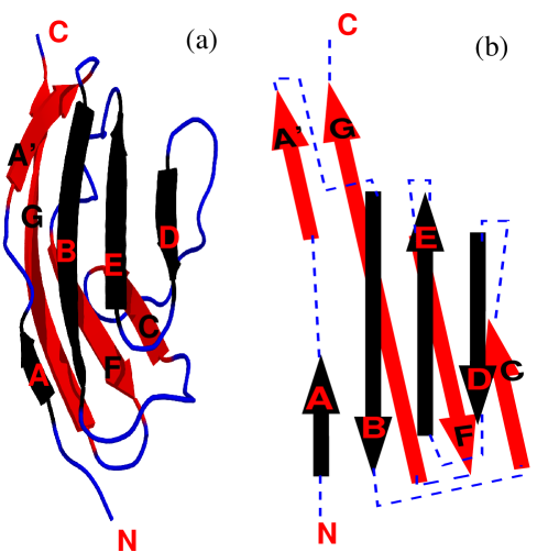
Figure 1: Native state conformation of the I27 domain of titin (PDB ID: 1TIT). There are 8 $\beta$-strands: A (4-7), A’ (11-15), B (18-25), C (32-36), D (47-52), E (55-61), F(69-75) and G (78-88). (a) PDB structure in cartoon representation. (b) Schematic view of the same structure. Red and black $\beta$-strands belong to different $\beta$-sheets. N- and C-terminal residues are marked N and C, respectively.

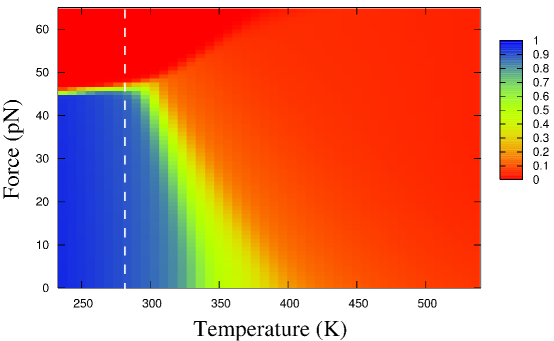
Figure 2: The $f-T$ phase diagram obtained by the extended histogram method. The results were averaged over 30 trajectories. The vertical dashed line marks $T=0.42\epsilon_{H}/k_{B}=280$ K at which most of our calculations have been performed.

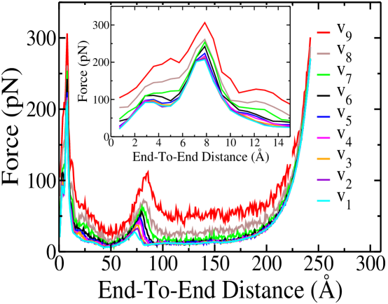
Figure 3: Averaged force-extension profiles of the I27 titin domain. The results obtained by Go-model simulations performed at different pulling speeds are shown on the right. The inset shows an enlargement of the starting region. Results have been averaged over 50 trajectories. Values of pulling rates are given in Table 1.

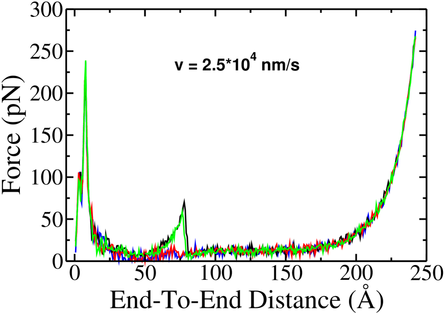
Figure 4: Individual force-extension profiles of the I27 titin domain. Four individual trajectories at $2.5\times 10^{4}$ nm/s obtained by Go-model simulations are presented. There is no second peak in two trajectories.

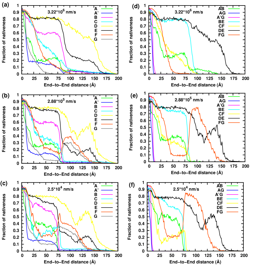
Figure 5: End-to-end distance dependence of averaged fractions of native contacts. Native contacts are formed by 8 $\beta$-strands marked in Fig. 1 at different loading rates. Clearly, the unfolding at high forces starts from the C-termin us detaching G-strand first. In contrast, at low forces the A and A’ strands are unfolded first, but it should be noted that the extension at which complete detachment of the A strand takes place is rather large, $75~{}\mathrm{\mathring{A}}$.

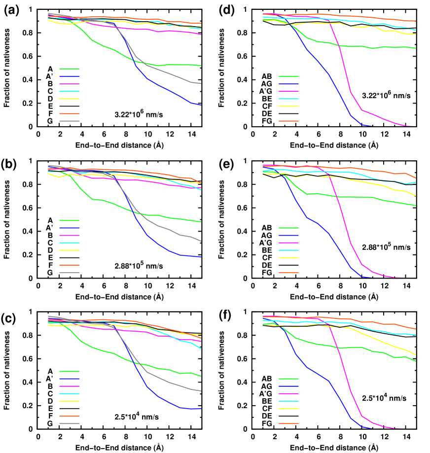
Figure 6: End-to-end distance dependence of averaged fractions of native contacts. Same as Fig. 5 but for the end-to-end distance up to 15 $\AA$. Within $15\mathring{A}$ the detachment of the A strand out of the protein core is not observed for any speed studied.

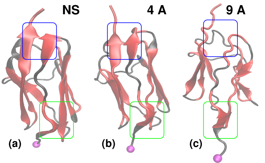
Figure 7: Typical unfolding pathway of titin from Go-model simulation. Green and blue squares mark AB and A’G regions, respectively. The N-terminal residue is shown in magenta. (a) NS conformation. (b) Conformation at $4\mathring{A}$ extension, contacts between AG are missing, both A’G and AB remained formed. (c) Conformation at $9\mathring{A}$ extension (after the main peak), contacts between G with A and A’ are broken, those between the A and B strands are preserved. It should be emphasized that 100$\%$ trajectories at the beginning of unfolding (within $10\mathring{A}$) proceed via the same pathway presented here regardless of the applied pulling rate.

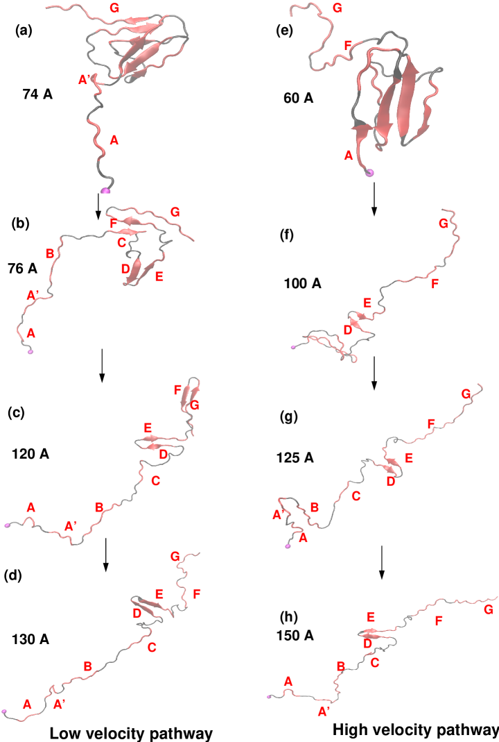
Figure 8: Typical unfolding pathways of titin. (a-d) High pulling speed and (e-h) low pulling speed regions. The N-terminal residue is shown in magenta.

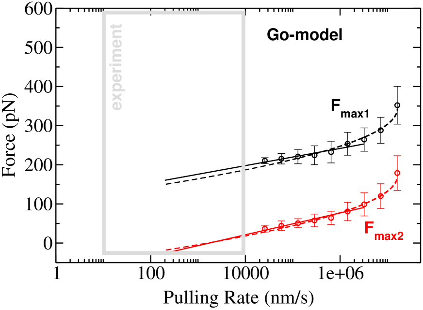
Figure 9: Force dependence on pulling speeds at $T=285K$. Force at a given value of pulling speed is computed as an average of maximum forces over 50 trajectories. Grey boundaries of the polygon illustrate the interval of pulling rates used in the AFM experiment. Black circles correspond to data for $F_{max1}$. Solid and dashed black curves represent linear and nonlinear fits for $F_{max1}$. Similarly, red color is used for $F_{max2}$. Straight lines are fits to the Bell-Evans-Ritchie equation (Eq.7), $y=109.6+9.59\ln(x)$ and $y=-90.332+12.108\ln(x)$ for $F_{max1}$ and $F_{max2}$, respectively. Using a linear fit we found $x_{u(N\rightarrow TS1)}=3.76\mathring{A}$ and $x_{u(IS\rightarrow DS)}=2.95\mathring{A}$ for $F_{max1}$ and $F_{max2}$, respectively. From a nonlinear fit and Eq.8 we got $x_{u}=6.68\mathring{A}$ and $\Delta G^{\ddagger}=32.48k_{B}T$ for $F_{max1}$ and $x_{u}=3.88\mathring{A}$ and $\Delta G^{\ddagger}=9.22k_{B}T$ for $F_{max2}$. Extrapolation to the experimental pulling speed, $v=200$ nm/s, gives a negative value of $F_{max2}$ regardless of the fit used. Extrapolated values of $F_{max1}$ to $200$ nm/s are 160 and 152 pN using linear and nonlinear fits, respectively.