Curvilinear Grids for WENO Methods in Astrophysical Simulations

Abstract

We investigate the applicability of curvilinear grids in the context of astrophysical simulations and WENO schemes. With the non-smooth mapping functions from Calhoun et al. [1], we can tackle many astrophysical problems which were out of scope with the standard grids in numerical astrophysics. We describe the difficulties occurring when implementing curvilinear coordinates into our WENO code, and how we overcome them. We illustrate the theoretical results with numerical data. The WENO finite difference scheme works only for high Mach number flows and smooth mapping functions whereas the finite volume scheme gives accurate results even for low Mach number flows and on non-smooth grids.

1 Introduction

There are many astrophysical applications where the physical domain of interest is a sphere or a circle, e.g. the numerical simulation of core convection [2, 3] or of convection in giant planets [4, 5]. The usability of spherical coordinate systems is restricted due to the grid singularity in the centre of the sphere as discussed, for instance, by Evonuk and Glatzmaier [5]. With a Cartesian grid, a huge part of the computational resources are wasted [6] and to improve resolution along spheres, complex adaptive mesh refinements have to be used [7] to keep the computational requirements manageable. Therefore, all default grids used in numerical astrophysics have some fatal deficiencies.

For the specific case of a sphere with grid singularity at the centre, Cai et al. [3] proposed a different approach. They use spectral expansion methods on a spherical grid. To avoid the time step restriction due to converging grid lines at the centre, they lower the order of the harmonic expansion at the centre. The equations are recast in a form such that boundary conditions can easily be applied at the centre. In this way, the simulation domain can be extended to the full sphere. Anyway, their procedure still requires the specification of a boundary condition at the centre and applies only to spherical domains.

Mocz et al. [8] implemented a discontinuous Galerkin method on arbitrary static and moving Voronoi meshes. In theory, their approach promises great flexibility and wide applicability. In applications, however, there are still numerical difficulties present, e.g. in the treatment of shocks, making the use of the method in astrophysical applications difficult at the moment.

In this paper, we present the methods used to extend the applicability of the simulation code ANTARES [9] to more general geometries. Until now, ANTARES was exclusively applied to numerical simulations of solar and stellar surface convection and stellar interiors in Cartesian geometry [e.g., 9, 10] as well as convection in Cepheids in spherical geometry [e.g., 11, 12]. For the inviscid part of the Navier–Stokes equations, the WENO finite difference scheme is employed [13, 14, 15]. The WENO scheme is a highly efficient shock-capturing scheme which can be implemented at several different orders of accuracy. In this paper, we consider the fifth order variant called WENO5. Its superiority compared to other high-order schemes was shown, e.g., in Muthsam et al. [16]. Nevertheless, its applicability is restricted by its specific requirements concerning the grid geometry [15].

The technique of curvilinear or mapped grids is widely used in engineering [17, 18, 19], but until now was only seldomly applied in an astrophysical setting [20]. In principle, given a suitable mapping function, any problem defined on a general domain can be transformed into a problem in a computational space which is equidistant and Cartesian and where any standard numerical scheme, the applicability of which often is restricted to Cartesian and equidistant grids, can be used. The only requirement is that the grid in physical space is structured.

In the context of curvilinear coordinates, Calhoun et al. [1] presented several functions mapping spherical domains to the Cartesian computational domain. These functions are not strongly differentiable and were mainly applied in engineering applications until now.

In this paper, we will show how well the WENO finite difference and finite volume scheme performs on smooth and non-smooth grids for flows in the intermediate flow regime of $0.1\leq{\rm Ma}\leq 1$ typical for many problems in stellar astrophysics. We will call a grid (non)smooth if the associated mapping function is (non)smooth.

Shu [14] applied the WENO finite difference scheme in a straightforward way to smooth grids. In all numerical examples in the mentioned paper, the Mach number ${\rm Ma}=\frac{\left|u\right|}{v_{\rm snd}}$ was higher than $1$. The behaviour of the method in the low Mach number limit on Cartesian grids was investigated in Happenhofer et al. [10]. They showed that the WENO5 finite difference scheme does not perform well for Mach numbers smaller than $0.1$ even on Cartesian grids.

Most of the findings of this paper are not restricted to our specific code, but apply to any finite difference or finite volume code. From the numerical experiments in Section 3, we conclude in which situations and in which numerical setup the mapped grid technique gives reliable results. Thereby, we concentrate on the WENO algorithm and on astrophysical simulations. We demonstrate the usefulness and applicability of the mapping functions for a sphere from Calhoun et al. [1] in this setting.

1.1 WENO Finite Difference and Finite Volume Formulation

The Euler equations are a system of partial differential equations. In two spatial dimensions and in a Cartesian coordinate system, their differential form is

$$\frac{\partial}{\partial t}{\bf Q}+\frac{\partial}{\partial x}{\bf F}+\frac{\partial}{\partial y}{\bf G}=0,$$ (1)

with the state vector ${\bf Q}$ and the flux functions ${\bf F}$ and ${\bf G}$ given by

$${\bf Q}=\left(\begin{array}[]{c}\rho\\ \rho u\\ \rho v\\ E\end{array}\right),{\bf F}\left({\bf Q}\right)=\left(\begin{array}[]{c}\rho u\\ \rho u^{2}+p\\ \rho uv\\ (p+E)u\end{array}\right),{\bf G}\left({\bf Q}\right)=\left(\begin{array}[]{c}\rho v\\ \rho vu\\ \rho v^{2}+p\\ (p+E)v\end{array}\right),$$ (2)

where the pressure $p=p(\rho,e)$ is given by an equation of state and $e=E-\frac{u^{2}+v^{2}+w^{2}}{2\rho}$ is the internal energy. In the following, we will write ${\bf u}:=\left(u,v\right)^{T}$ for the velocity vector.

We discretise the Euler equations as described in A and in Merriman [15] for the case of an equidistant Cartesian grid. In the finite difference case, the fluxes are reconstructed directly, whereas in the finite volume case, the conservative variables are reconstructed. The procedure is described in pseudo code in Algorithms 1 and 2.

Algorithm 1 Finite difference scheme for the two-dimensional Euler equations.

1:  ${\bf Q}_{i,j}$ is given as point value at the cell centre.

2:  $\mathrm{A}({\bf f})_{i,j}={\bf F}_{i,j}$, $\mathrm{A}({\bf g})_{i,j}={\bf G}_{i,j}$

3:  ${\bf f}_{i\pm\frac{1}{2},j}=\mathrm{R}_{x}\left({\bf F}_{i,j}\right)$, ${\bf g}_{i,j\pm\frac{1}{2}}=\mathrm{R}_{y}\left({\bf G}_{i,j}\right)$

4:  $\frac{\partial{\bf Q}_{i,j}}{\partial t}=-\frac{1}{\delta x}\left({\bf f}_{i+\frac{1}{2},j}-{\bf f}_{i-\frac{1}{2},j}\right)-\frac{1}{\delta y}\left({\bf g}_{i,j+\frac{1}{2}}-{\bf g}_{i,j-\frac{1}{2}}\right)$

Algorithm 2 Finite volume scheme for the two-dimensional Euler equations.

1:  ${\bf Q}_{i,j}={\bf\overline{Q}}_{i,j}$ is given as cell average.

2:  ${\bf Q}_{i\pm\frac{1}{2},j}=\mathrm{R}_{x}\left({\bf\overline{Q}}_{i,j}\right)$, ${\bf Q}_{i,j\pm\frac{1}{2}}=\mathrm{R}_{y}\left({\bf\overline{Q}}_{i,j}\right)$

3:  ${\bf F}_{i\pm\frac{1}{2},j}={\bf F}\left({\bf Q}_{i\pm\frac{1}{2},j}\right)$, ${\bf G}_{i,j\pm\frac{1}{2}}={\bf G}\left({\bf Q}_{i,j\pm\frac{1}{2}}\right)$

4:  $\frac{\partial{\bf\overline{Q}}_{i,j}}{\partial t}=-\frac{1}{\delta x}\left({\bf F}_{i+\frac{1}{2},j}-{\bf F}_{i-\frac{1}{2},j}\right)-\frac{1}{\delta y}\left({\bf G}_{i,j+\frac{1}{2}}-{\bf G}_{i,j-\frac{1}{2}}\right)$

Both algorithms need the specification of a reconstruction operator. A reconstruction operator calculates the point value of a function given its cell averages. The WENO reconstruction operator is described, e.g., in Shu [14] and C. In the derivation of the finite difference scheme, we required the grid to be equidistant. The fluxes in the finite volume scheme are second-order approximations to the analytical fluxes which are line integrals over the cell boundary. Details can be found in A.

2 Mapped Grids

Numerical schemes which are designed for Cartesian, equidistant grids can be generalised to more complicated domains with the technique of mapped grids. There, a mapping function

$$M:\ \left[-1,1\right]^{2}\to\Omega,\ M(\xi,\eta)=(x,y)^{T},$$ (3)

is defined which maps the Cartesian and equidistant computational space into the physical space. The information about the geometry of the physical space is then contained in the transformed partial differential equations. The Euler equations in strong conservation form in physical space (1) are transformed into strong conservation form in computational space. In two dimensions, they take the form

$$\frac{\partial}{\partial t}J^{-1}{\bf Q}+\frac{\partial}{\partial\xi}{\bf\hat{F}}+\frac{\partial}{\partial\eta}{\bf\hat{G}}=0$$ (4a)

with

$${\bf\hat{F}}= \frac{\partial y}{\partial\eta}{\bf F}-\frac{\partial x}{\partial\eta}{\bf G},$$ (4b)

$${\bf\hat{G}}= -\frac{\partial y}{\partial\xi}{\bf F}+\frac{\partial x}{\partial\xi}{\bf G},$$ (4c)

where $J^{-1}$ is the determinant of the inverse Jacobian of the mapping function $M$ [see, e.g., 20]. $\xi$ and $\eta$ are the computational variables defined by the mapping function $M$.

We present two derivations of the strong conservation form of the two-dimensional Euler equations in computational space (2) which differ in their differentiability assumptions concerning the mapping function $M$. The classical first approach assuming strong differentiability of the mapping function can be found in B. A more general derivation is sketched out in the following section.

In applications, the mapping function $M$ which maps the computational domain into the physical domain $\Omega$ is unknown or does not possess an analytical form. We therefore seek for a derivation of the transformed equations (2) which does not require any differentiability of the mapping function $M$. Following the description in Wesseling [17], we assume that a structured set of nodes $(x_{i\pm\frac{1}{2},j\pm\frac{1}{2}},y_{i\pm\frac{1}{2},j\pm\frac{1}{2}})$, $1\leq i\leq n$, $1\leq j\leq m$, is given [e.g., by an external grid generation program, see 21], instead of an analytical expression for $M$. $\Omega$ is the smallest region $R\subset\mathbb{R}^{2}$ such that $(x_{i\pm\frac{1}{2},j\pm\frac{1}{2}},y_{i\pm\frac{1}{2},j\pm\frac{1}{2}})\in\overline{R}\ \forall i,j$, where $\overline{R}$ is the closure of $R$. Then we define the discrete mapping function $\tilde{M}$ point-wisely by

$$\tilde{M}(\xi_{i-\frac{1}{2}},\eta_{j-\frac{1}{2}})=(x_{i-\frac{1}{2},j-\frac{1}{2}},y_{i-\frac{1}{2},j-\frac{1}{2}}),i=1,\ldots,n+1,j=1,\ldots,m+1.$$ (5)

For $(\xi,\eta)\in C_{i,j}:=\left[\xi_{i-\frac{1}{2}},\xi_{i+\frac{1}{2}}\right]\times\left[\eta_{j-\frac{1}{2}},\eta_{j+\frac{1}{2}}\right]$, we define $M(\xi,\eta)$ by bilinear interpolation of the physical coordinates of the edges of the cell. In this way, we continue $\tilde{M}$ to $M:\ \left[-1,1\right]\times\left[-1,1\right]\to\Omega$. $M$ is continuous, linear in each $C_{i,j}$, but not differentiable on the boundary of each cell $C_{i,j}$. It follows that $M\not\in C^{1}(\left[-1,1\right]^{2})$, but $M\in H^{1}(\left[-1,1\right]^{2})$.

If the mapping function is defined in this way, the image of each cell $C_{i,j}$ is a quadrilateral $D_{i,j}$ with edges $\left(x_{i-\frac{1}{2},j-\frac{1}{2}},y_{i-\frac{1}{2},j-\frac{1}{2}}\right)$, $\left(x_{i-\frac{1}{2},j+\frac{1}{2}},y_{i-\frac{1}{2},j+\frac{1}{2}}\right)$, $\left(x_{i+\frac{1}{2},j-\frac{1}{2}},y_{i+\frac{1}{2},j-\frac{1}{2}}\right)$, and $\left(x_{i+\frac{1}{2},j+\frac{1}{2}},y_{i+\frac{1}{2},j+\frac{1}{2}}\right)$ in physical space. All cell sides are straight lines. We can choose the quadrilateral $D_{i,j}$ as the (arbitrary) control volume $W\subset\Omega$ of the integral formulation of the Euler equations

$$\frac{\partial}{\partial t}\int_{W}\rho\,dV= -\int_{\partial W}{\bf n}\cdot\rho{\bf u}\,dA,$$ (6a)

$$\frac{\partial}{\partial t}\int_{W}\rho{\bf u}\,dV= -\int_{\partial W}\left[{\bf n}\cdot\rho{\bf u}\otimes{\bf u}+{\bf n}p\right]\,dA,$$ (6b)

$$\frac{\partial}{\partial t}\int_{W}E\,dV= -\int_{\partial W}{\bf n}\cdot\left(p+E\right){\bf u}\,dA,$$ (6c)

where ${\bf n}$ is the unit outward normal on $\partial W$, the boundary of $W$. Due to Gauss’ Theorem [p. 627, 22], equations (6) are equivalent to the differential form (1) for sufficiently smooth functions [23]. But $\partial W=\partial D_{i,j}$ consists of the four straight lines

$$S_{i\pm\frac{1}{2}} =\left(\begin{array}[]{c}x_{i\pm\frac{1}{2},j+\frac{1}{2}}\\ y_{i\pm\frac{1}{2},j+\frac{1}{2}}\end{array}\right)-\left(\begin{array}[]{c}x_{i\pm\frac{1}{2},j-\frac{1}{2}}\\ y_{i\pm\frac{1}{2},j-\frac{1}{2}}\end{array}\right),$$ (7e)

$$S_{j\pm\frac{1}{2}} =\left(\begin{array}[]{c}x_{i+\frac{1}{2},j\pm\frac{1}{2}}\\ y_{i+\frac{1}{2},j\pm\frac{1}{2}}\end{array}\right)-\left(\begin{array}[]{c}x_{i-\frac{1}{2},j\pm\frac{1}{2}}\\ y_{i-\frac{1}{2},j\pm\frac{1}{2}}\end{array}\right).$$ (7j)

Their length is given by

$$\left|S_{i\pm\frac{1}{2}}\right| =\sqrt{\left(x_{i\pm\frac{1}{2},j+\frac{1}{2}}-x_{i\pm\frac{1}{2},j-\frac{1}{2}}\right)^{2}+\left(y_{i\pm\frac{1}{2},j+\frac{1}{2}}-y_{i\pm\frac{1}{2},j-\frac{1}{2}}\right)^{2}},$$ (8a)

$$\left|S_{j\pm\frac{1}{2}}\right| =\sqrt{\left(x_{i+\frac{1}{2},j\pm\frac{1}{2}}-x_{i-\frac{1}{2},j\pm\frac{1}{2}}\right)^{2}+\left(y_{i+\frac{1}{2},j\pm\frac{1}{2}}-y_{i-\frac{1}{2},j\pm\frac{1}{2}}\right)^{2}},$$ (8b)

and the normal vectors ${\bf n}=\left(\begin{array}[]{c}n_{1}\\ n_{2}\end{array}\right)$ in equations (6) are exactly

$$n_{1} =\left(y_{i\pm\frac{1}{2},j+\frac{1}{2}}-y_{i\pm\frac{1}{2},j-\frac{1}{2}}\right)/\left|S_{i\pm\frac{1}{2}}\right|,$$ (8c)

$$n_{2} =-\left(x_{i\pm\frac{1}{2},j+\frac{1}{2}}-x_{i\pm\frac{1}{2},j-\frac{1}{2}}\right)/\left|S_{i\pm\frac{1}{2}}\right|$$ (8d)

on $S_{i\pm\frac{1}{2}}$ and

$$n_{1} =-\left(y_{i+\frac{1}{2},j\pm\frac{1}{2}}-y_{i-\frac{1}{2},j\pm\frac{1}{2}}\right)/\left|S_{j\pm\frac{1}{2}}\right|,$$ (8e)

$$n_{2} =\left(x_{i+\frac{1}{2},j\pm\frac{1}{2}}-x_{i-\frac{1}{2},j\pm\frac{1}{2}}\right)/\left|S_{j\pm\frac{1}{2}}\right|.$$ (8f)

on $S_{j\pm\frac{1}{2}}$. From now on, we will write ${\bf n}=\left(\begin{array}[]{c}n_{1}\\ n_{2}\end{array}\right)$ for the normal vector on $S_{i\pm\frac{1}{2}}$ and ${\bf m}=\left(\begin{array}[]{c}m_{1}\\ m_{2}\end{array}\right)$ for the normal vector on $S_{j\pm\frac{1}{2}}$. The surface area of the quadrilateral $D_{i,j}$ is

$$\left|D_{i,j}\right|= \frac{1}{2}\Big{|}(y_{i-\frac{1}{2},j-\frac{1}{2}}-y_{i+\frac{1}{2},j+\frac{1}{2}})(x_{i-\frac{1}{2},j+\frac{1}{2}}-x_{i+\frac{1}{2},j-\frac{1}{2}})$$

$$+(y_{i+\frac{1}{2},j-\frac{1}{2}}-y_{i-\frac{1}{2},j+\frac{1}{2}})(x_{i-\frac{1}{2},j-\frac{1}{2}}-x_{i+\frac{1}{2},j+\frac{1}{2}})\Big{|}.$$

Since $\left|D_{i,j}\right|>0$, we define the cell average of the state vector ${\bf Q}_{i,j}$ in the cell $(i,j)$ by

$$\overline{\bf Q}_{i,j}=\left|D_{i,j}\right|^{-1}\int_{D_{i,j}}{\bf Q}\,dV.$$ (9)

With $U:=n_{1}u+n_{2}v$, $V:=m_{1}u+m_{2}v$, we can write equations (6) as

$$\frac{\partial}{\partial t}\overline{\bf Q}_{i,j}=-\left(\int_{S_{i+\frac{1}{2}}}{\bf\hat{F}}\,dS-\int_{S_{i-\frac{1}{2}}}{\bf\hat{F}}\,dS+\int_{S_{j+\frac{1}{2}}}{\bf\hat{G}}\,dS-\int_{S_{j-\frac{1}{2}}}{\bf\hat{G}}\,dS\right),$$ (10)

where

$${\bf Q}=\left(\begin{array}[]{c}\rho\\ \rho u\\ \rho v\\ E\end{array}\right),{\bf\hat{F}}=\left(\begin{array}[]{c}\rho U\\ \rho Uu+n_{1}p\\ \rho Uv+n_{2}p\\ (p+E)U\end{array}\right),{\bf\hat{G}}=\left(\begin{array}[]{c}\rho V\\ \rho Vu+m_{1}p\\ \rho Vu+m_{2}p\\ (p+E)V\end{array}\right).$$ (11)

Evaluating the line integrals in (10) with the midpoint rule, we get

$$\frac{\partial}{\partial t}\left|D_{i,j}\right|\overline{\bf Q}_{i,j}=-\left({\bf\hat{F}}_{i+\frac{1}{2},j}-{\bf\hat{F}}_{i-\frac{1}{2},j}+{\bf\hat{G}}_{i,j+\frac{1}{2}}-{\bf\hat{G}}_{i,j-\frac{1}{2}}\right).$$ (12)

In the computational space, all standard numerical methods can be used to calculate the value of the numerical flux functions ${\bf\hat{F}}$ and ${\bf\hat{G}}$ since the computational space is equidistant and Cartesian. In particular, both the finite difference and the finite volume WENO scheme as described in Algorithms 1 and 2 can be applied to solve (12). The specific form of the algorithms for curvilinear coordinates can be found in Algorithms 3 and 4.

Algorithm 3 Finite difference scheme for curvilinear coordinates.

1:  ${\bf Q}_{i,j}$ is given as point value at the cell centre.

2:  $\mathrm{A}({\bf\hat{f}})_{i,j}={\bf\hat{F}}_{i,j}={n_{1}}|_{i,j}{\bf F}_{i,j}+{n_{2}}|_{i,j}{\bf G}_{i,j}$, $\mathrm{A}({\bf\hat{g}})_{i,j}={\bf\hat{G}}_{i,j}={m_{1}}|_{i,j}{\bf F}_{i,j}+{m_{2}}|_{i,j}{\bf G}_{i,j}$

3:  ${\bf\hat{f}}_{i\pm\frac{1}{2},j}=\mathrm{R}_{\xi}\left({\bf\hat{F}}_{i,j}\right)$, ${\bf\hat{g}}_{i,j\pm\frac{1}{2}}=\mathrm{R}_{\eta}\left({\bf\hat{G}}_{i,j}\right)$

4:  $\frac{\partial{\bf Q}_{i,j}}{\partial t}=-\frac{1}{\delta\xi}\left({\bf\hat{f}}_{i+\frac{1}{2},j}-{\bf\hat{f}}_{i-\frac{1}{2},j}\right)-\frac{1}{\delta\eta}\left({\bf\hat{g}}_{i,j+\frac{1}{2}}-{\bf\hat{g}}_{i,j-\frac{1}{2}}\right)$

Algorithm 4 Finite volume scheme for curvilinear coordinates.

1:  ${\bf Q}_{i,j}={\bf\overline{Q}}_{i,j}$ is given as cell average.

2:  ${\bf Q}_{i\pm\frac{1}{2},j}=\mathrm{R}_{\xi}\left({\bf\overline{Q}}_{i,j}\right)$, ${\bf Q}_{i,j\pm\frac{1}{2}}=\mathrm{R}_{\eta}\left({\bf\overline{Q}}_{i,j}\right)$

3:  ${\bf\hat{F}}_{i\pm\frac{1}{2},j}={n_{1}}|_{i\pm\frac{1}{2},j}{\bf F}\left({\bf Q}_{i\pm\frac{1}{2},j}\right)+{n_{2}}|_{i\pm\frac{1}{2},j}{\bf G}\left({\bf Q}_{i\pm\frac{1}{2},j}\right)$, ${\bf\hat{G}}_{i,j\pm\frac{1}{2}}={m_{1}}|_{i,j\pm\frac{1}{2}}{\bf F}\left({\bf Q}_{i,j\pm\frac{1}{2}}\right)+{m_{2}}|_{i,j\pm\frac{1}{2}}{\bf G}\left({\bf Q}_{i,j\pm\frac{1}{2}}\right)$

4:  $\frac{\partial{\bf\overline{Q}}_{i,j}}{\partial t}=-\frac{1}{\delta\xi}\left({\bf\hat{F}}_{i+\frac{1}{2},j}-{\bf\hat{F}}_{i-\frac{1}{2},j}\right)-\frac{1}{\delta\eta}\left({\bf\hat{G}}_{i,j+\frac{1}{2}}-{\bf\hat{G}}_{i,j-\frac{1}{2}}\right)$

The advantage of the weak derivation, besides that it does not require $M$ to be differentiable, is that one gets formulae for all metric terms occurring in the transformation process. The Jacobian of the transformation is given by the area of the corresponding quadrilateral and therefore is positive by definition. The mapping function is not required to fulfil any smoothness properties. We therefore prefer to define our mapping function in this way.

We note that similar formulae exist for the three-dimensional case. The precise formulation can be found, e.g., in Visbal and Gaitonde [24].

2.1 Grids for Spherical Domains

There is no strongly differentiable function (a diffeomorphism) from the (unit) sphere to the (unit) square since the square is not a submanifold of $\mathbb{R}^{2}$. Therefore, if we want to use the mapped grid technique to perform simulations on spherical domains, we have to rely on mapping functions which are only weakly differentiable.

For the mapped grid technique, Calhoun et al. [1] gave some examples of mapping functions which map a circular domain to $\left[-1,1\right]^{2}$ and vice versa. In this paper, we want to investigate how the mapping functions $M_{1}$ and $M_{2}$ from Calhoun et al. [1] defined by

$$M_{1}:\ \left[-1,1\right]^{2}\to\Omega,\ x=R\cdot\frac{\max\left(\left|\xi\right|,\left|\eta\right|\right)\xi}{\sqrt{\xi^{2}+\eta^{2}}},$$ (13a)

$$y=R\cdot\frac{\max\left(\left|\xi\right|,\left|\eta\right|\right)\eta}{\sqrt{\xi^{2}+\eta^{2}}},$$ (13b)

$$M_{2}:\ \left[-1,1\right]^{2}\to\Omega,\ w=\max\left(\left|\xi\right|,\left|\eta\right|\right)^{2},$$ (13c)

$$x=w\cdot x_{M_{1}}+(1-w)\cdot\frac{R\xi}{\sqrt{2}},$$ (13d)

$$y=w\cdot y_{M_{1}}+(1-w)\cdot\frac{R\eta}{\sqrt{2}},$$ (13e)

where $x_{M_{1}}$ and $y_{M_{1}}$ are the physical coordinates defined by $M_{1}$, and

$$\Omega=\{\left(x,y\right)\in\mathbb{R}^{2}:\sqrt{x^{2}+y^{2}}\leq R\},$$ (14)

perform in numerical simulations when WENO schemes are employed.

It is obvious to see that these functions are only weakly differentiable. Therefore, they should be applied only in the context of the methods developed in Section 2.

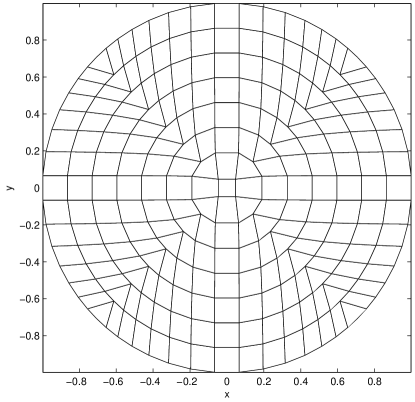
Figure 1: Grid defined by function $M_{1}$ from Calhoun et al. [1].

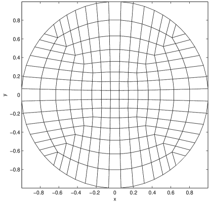
Figure 2: Grid defined by function $M_{2}$ from Calhoun et al. [1].

2.2 Freestream Problem

Nonomura et al. [25] emphasize the importance of the following, seemingly simple, test problem.

Problem 1 (Freestream preservation for the Euler equations).

Given the initial conditions

$$\left(\rho,\rho u,\rho v,E\right)=\left(\rho_{0},0,0,e_{0}\right),$$ (15)

with constant density $\rho_{0}$ and internal energy $e_{0}$, the numerical solution of the transformed system (2) should stay close to the analytical solution

$$\left(\rho,\rho u,\rho v,E\right)=\left(\rho_{0},0,0,e_{0}\right)$$ (16)

for all times. $p_{0}=p(\rho_{0},e_{0})$ is the pressure given by the equation of state.

Plugging these initial conditions into the transformed Euler equations (2), we get

$$0=p_{0}\left(\frac{\partial n_{1}}{\partial\xi}+\frac{\partial m_{1}}{\partial\eta}\right),\ 0=p_{0}\left(\frac{\partial n_{2}}{\partial\xi}+\frac{\partial m_{2}}{\partial\eta}\right),$$ (17)

since $\frac{\partial}{\partial t}\left(\rho u\right)=\frac{\partial}{\partial t}\left(\rho v\right)=0$. This condition must be fulfilled numerically in order to prevent numerical errors. Since

$$n_{1}=\frac{\partial y}{\partial\eta},n_{2}=-\frac{\partial x}{\partial\eta},m_{1}=-\frac{\partial y}{\partial\xi},m_{2}=\frac{\partial x}{\partial\xi},$$ (18)

this is equivalent to the requirement that the second derivatives of the mapping function $M$ are symmetric. Every function which is twice (weakly) differentiable fulfils this property.

Next, we investigate if the freestream is preserved by the finite difference and the finite volume discretisation of the Euler equations. The WENO finite difference scheme as summarised in Algorithm 3 corresponds to the scheme WENO-G in Nonomura et al. [25]. In the cited reference, they describe precisely why the finite difference scheme does not fulfil the freestream preservation property. The fluxes $\hat{\bf F}$ and $\hat{\bf G}$ are reconstructed directly from their value at the cell centre, including the metric terms evaluated at the cell centre. These fluxes are not constant for the freestream initial conditions. The reconstructed fluxes at the cell boundary will not be constant, too, and be different on any cell boundary. Therefore, they will not cancel out, and steadily, a numerical error is introduced.

We note that Nonomura et al. [25] introduced the WENO-C scheme as a different WENO finite difference scheme which fulfils the freestream property by calculating $\frac{\partial\bf Q}{\partial t}$ via

$$\frac{\partial\bf Q}{\partial t}=\frac{\partial\xi}{\partial x}\frac{\partial\bf F}{\partial\xi}+\frac{\partial\eta}{\partial x}\frac{\partial\bf F}{\partial\eta}+\frac{\partial\xi}{\partial y}\frac{\partial\bf G}{\partial\xi}+\frac{\partial\eta}{\partial y}\frac{\partial\bf G}{\partial\eta}.$$ (19)

We did not consider this scheme in our paper since it is not conservative and its computational costs are three times higher than WENO-G in three dimensions, making the scheme useless for our purposes.

On the contrary, for the WENO finite volume scheme as summarised in Algorithm 4, the state vector ${\bf Q}$ is reconstructed at the cell boundaries from its cell averages. Therefore, for Problem 1 the reconstruction process will yield constant approximations for the state vector at the cell interface, i.e.

$${\bf Q}_{i\pm\frac{1}{2},j}={\bf Q}_{i,j\pm\frac{1}{2}}=\left(\rho_{0},0,0,e_{0}\right)^{T}.$$ (20)

In the update step (12), only the metric terms will be non-constant. In precise terms, the conditions

$$\frac{n_{1}|_{i+\frac{1}{2},j}-n_{1}|_{i-\frac{1}{2},j}}{\delta\xi}+\frac{m_{1}|_{i,j+\frac{1}{2}}-m_{1}|_{i,j-\frac{1}{2}}}{\delta\eta}=0,$$ (21a)

$$\frac{n_{2}|_{i+\frac{1}{2},j}-n_{2}|_{i-\frac{1}{2},j}}{\delta\xi}+\frac{m_{2}|_{i,j+\frac{1}{2}}-m_{2}|_{i,j-\frac{1}{2}}}{\delta\eta}=0,$$ (21b)

are equivalent to preserving the freestream. If the metric terms are calculated, as described in Section 2, by

$$n_{1}|_{i\pm\frac{1}{2},j}= \frac{\partial y}{\partial\eta}|_{i\pm\frac{1}{2},j}=\frac{y_{i\pm\frac{1}{2},j+\frac{1}{2}}-y_{i\pm\frac{1}{2},j-\frac{1}{2}}}{\delta\eta},$$ (22a)

$$n_{2}|_{i\pm\frac{1}{2},j}= -\frac{\partial x}{\partial\eta}|_{i\pm\frac{1}{2},j}=-\frac{x_{i\pm\frac{1}{2},j+\frac{1}{2}}-x_{i\pm\frac{1}{2},j-\frac{1}{2}}}{\delta\eta},$$ (22b)

$$m_{1}|_{i,j\pm\frac{1}{2}}= -\frac{\partial y}{\partial\xi}|_{i,j\pm\frac{1}{2}}=-\frac{y_{i+\frac{1}{2},j\pm\frac{1}{2}}-y_{i-\frac{1}{2},j\pm\frac{1}{2}}}{\delta\xi},$$ (22c)

$$m_{2}|_{i,j\pm\frac{1}{2}}= \frac{\partial x}{\partial\xi}|_{i,j\pm\frac{1}{2}}=\frac{x_{i+\frac{1}{2},j\pm\frac{1}{2}}-x_{i-\frac{1}{2},j\pm\frac{1}{2}}}{\delta\xi},$$ (22d)

conditions (21) are fulfilled exactly and the freestream will be preserved numerically.

We note that the freestream is never preserved in general if analytical expressions for the metric terms are used (if available).

We remark that even though conditions (22) look like second-order approximations, they are rather analytical requirements which must be fulfilled by the discretisation of the metric terms in order to preserve the freestream. They are a consequence of the conservative discretisation of the derivatives in equations (1). As described in A, the discrete formulations of the Euler equations as in (31) and (34) are analytically equivalent to (1).

For trivial mapping functions such as $M:\ \left[-1,1\right]^{2}\to\left[-1,1\right]^{2}$, $M(\xi,\eta)=(\xi,\eta)^{T}$ with $\frac{\partial y}{\partial\eta}=\frac{\partial x}{\partial\xi}={\rm const}$, $\frac{\partial y}{\partial\xi}=\frac{\partial x}{\partial\eta}=0$, freestream preservation is of course possible even for the finite difference scheme WENO-G.

We conclude that the mapped grid technique should be used only with the WENO finite volume scheme and with the metric terms calculated by (21). Non-preservation of the freestream leads to inacceptable errors, as we will demonstrate in the following section. The WENO finite difference scheme cannot preserve the freestream and be conservative at the same time.

3 Numerical Results

In the following, we illustrate the theoretical results from the preceeding sections by numerical simulations. Besides the mapping functions $M_{1}$ and $M_{2}$ defined in (13), we use the mapping functions

$$M_{3}:\ \left[-1,1\right]^{2}\to\Omega,\ \begin{split}&x=-R+2R\cdot\left(\xi+0.1\sin\left(2\pi\xi\right)\sin\left(2\pi\eta\right)\right),\\ &y=-R+2R\cdot\left(\eta+0.1\sin\left(2\pi\xi\right)\sin\left(2\pi\eta\right)\right),\\ \end{split}$$ (23)

$$M_{4}:\ \left[-1,1\right]^{2}\to\Omega,\ \begin{split}&x=-R+2R\cdot\xi,\\ &y=-R+2R\cdot\eta,\end{split}$$ (24)

where $\Omega=\left[-R,R\right]^{2}$. $M_{3}$ was used in Colella et al. [26] to test the order of accuracy of their scheme since it is a smooth function, whereas $M_{4}$ gives a Cartesian grid. We will call a grid “smooth” if the mapping function defining this grid is smooth.

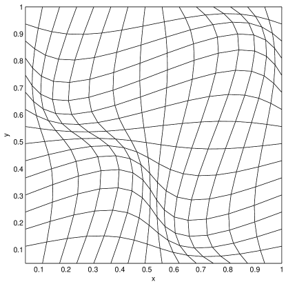
Figure 3: Grid defined by function $M_{3}$ from Colella et al. [26].

All simulations are performed with the code ANTARES [9] using explicit time integration schemes and Marquina flux splitting [27]. If not stated otherwise, the Runge–Kutta scheme employed in the simulations is SSP RK(3,2), a second-order Runge–Kutta scheme with three stages [28, 29]. In all simulations, the ideal gas equation is used, and the Courant number is fixed to $0.1$. The WENO finite difference scheme corresponds to the method WENO-G in Nonomura et al. [25].

3.1 Gresho Vortex

The specific setup of the Gresho Vortex used in this paragraph is described in Happenhofer et al. [10] and Miczek [30]. We repeat the definition here for convenience.

$$\rho= \,1,$$ (25a)

$$p_{0}= \,\frac{\rho}{\gamma\,{\rm Ma}_{\rm ref}^{2}},$$ (25b)

$$u_{\phi}= \begin{cases}5r,&0\leq r<0.2,\\ 2-5r,&0.2\leq r<0.4,\\ 0,&0.4\leq r,\end{cases},$$ (25c)

$$p= \begin{cases}p_{0}+\frac{25}{2}r^{2},&0\leq r<0.2,\\ p_{0}+\frac{25}{2}r^{2}+4(1-5r-\ln 0.2+\ln r),&0.2\leq r<0.4,\\ p_{0}-2+4\ln 2,&0.4\leq r.\end{cases}$$ (25d)

$r=\sqrt{x^{2}+y^{2}}$ is the distance from the origin and $u_{\phi}$ the angular velocity in terms of the polar angle $\phi=\texttt{atan2}(y,x)$. Note that the difference to the setup as it is described in Liska and Wendroff [31] is the introduction of a reference Mach number ${\rm Ma}_{\rm ref}$. The pressure $p$ is scaled such that the reference Mach number is the maximum Mach number of the resulting flow.

We performed a simulation with ${\rm Ma}_{\rm ref}=0.1$ and $\gamma=\frac{5}{3}$ over a time interval of $2\,{\rm s}$. The size of the domain is $1\,{\rm cm}$ in each direction, and we use $100\times 100$ grid points. The analytical solution is pure angular rotation of the vortex. The results on the four grids defined by the mapping functions $M_{1}$, $M_{2}$, $M_{3}$ and $M_{4}$ are shown in Figure 4 for the finite difference scheme and in Figure 5 for the finite volume scheme.

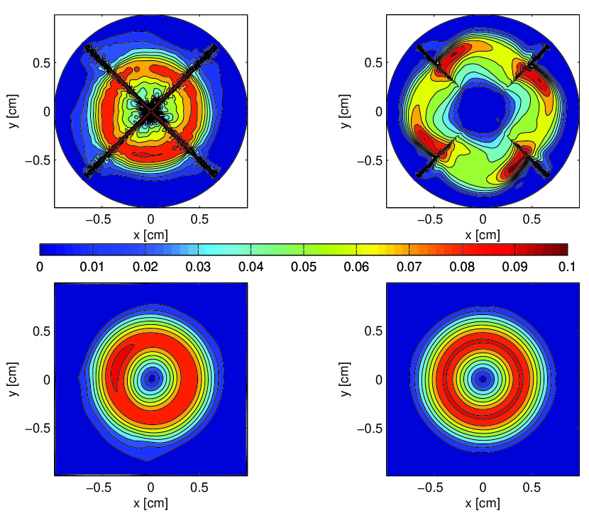
Figure 4: Mach number in the Gresho vortex test after $2\,{\rm s}$ with the WENO finite difference scheme. The initial Mach number was $0.1$. In all figures, the results of the simulation with $M_{1}$ are shown in the top left panel, with $M_{2}$ in the top right, with $M_{3}$ in the bottom left and with $M_{4}$ in the bottom right panel.

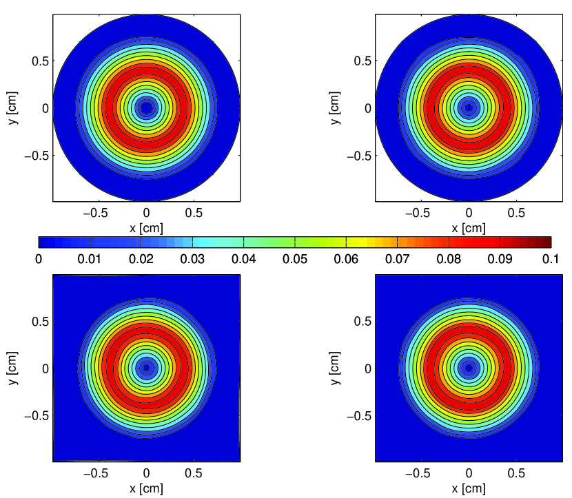
Figure 5: Mach number in the Gresho vortex test after $2\,{\rm s}$ with the WENO finite volume scheme. The initial Mach number was $0.1$.

With the non-smooth mapping functions $M_{1}$ and $M_{2}$, the results with the finite difference scheme are catastrophic, whereas with the finite volume scheme, the difference to the solution on the Cartesian grid is small. It is obvious that the problems come from the grid points where the mapping functions are not smooth. But even with the smooth mapping function $M_{3}$, the symmetry of the vortex is destroyed with the finite difference scheme, whereas there is no visible difference to the Cartesian solution with the finite volume scheme.

The Mach number ${\rm Ma}_{\rm ref}=0.1$ of this test is rather low for an explicit time integration scheme, but Happenhofer et al. [10] showed that the WENO scheme with Runge–Kutta time integration yields reliable results in this regime. As shown in Figure 6, the deformations due to the grid get smaller with higher Mach numbers, but in any case, the results with the finite volume scheme are more accurate. On the other hand, this explains why applying the mapped grid technique to the WENO finite difference scheme in Shu [14] worked properly: the mapping function were smooth, and the Mach number in the numerical tests was always larger than $1$.

We conclude that the WENO finite difference scheme should only be used in combination with the mapped grid technique if the mapping function is smooth and if the Mach number of the simulation is high. The reason for the bad performance lies in the violation of the preservation of the freestream. The finite volume scheme, however, yields accurate results even on non-smooth grids and in low Mach number tests.

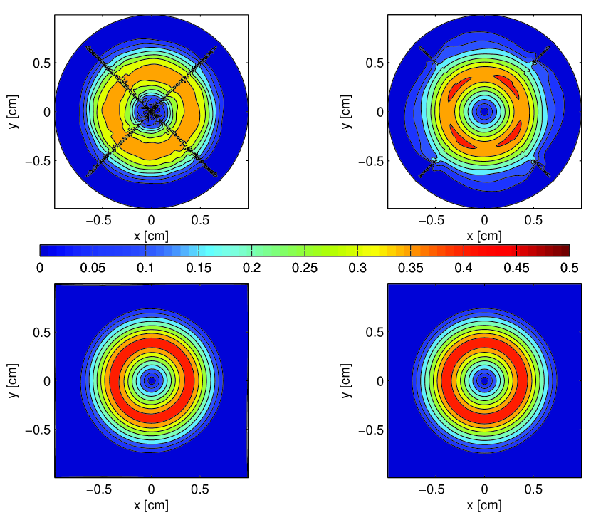
Figure 6: Mach number in the Gresho vortex test after $2\,{\rm s}$ with the WENO finite difference scheme with initial Mach number of $0.5$.

3.2 Sod Shock Tube

With the Sod Shock Tube [32] we test the performance of our schemes in the high Mach number regime. The computational domain is $\left[-0,5,0.5\right]^{2}$ and $\gamma=1.4$. In each direction, we use $100$ grid points. The inital shock position is at $0.2$ in $x$ direction.

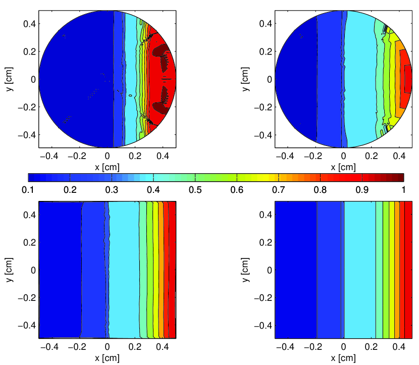
Figure 7: Density in the Sod Shocktube Test after $0.22\,{\rm s}$ with the WENO finite difference scheme. $M_{1}$ (top left panel) after $0.09\,{\rm s}$. In the outermost three layers, outflow boundary conditions are set.

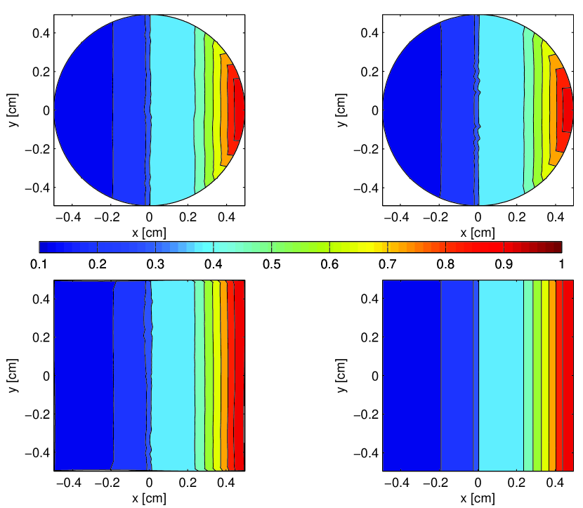
Figure 8: Density in the Sod Shocktube Test after $0.22\,{\rm s}$ with the WENO finite volume scheme. In the outermost three layers, outflow boundary conditions are set.

Even in this setup where the Mach number is rather high, the WENO finite difference scheme performs badly with the non-smooth mapping functions $M_{1}$ and $M_{2}$. With $M_{1}$, the simulation crashed after $0.09\,{\rm s}$ because of negative densities. At the diagonals, numerical artifacts occur even without any flow present at this position as a consequence of the violation of the freestream preservation.

The simulations with the finite volume scheme do not show any anomalies. On the smooth grids, the results from the two schemes are very similar.

3.3 Nonlinear Advection

Yee et al. [33], Zhang et al. [34] and Kifonidis and Müller [20] suggested a non-linear flow example to test the order of accuracy of a scheme. They showed that a smooth linear flow is not a suitable test case to test the accuracy of a finite volume method, because for a linear initial condition, the integration used to transform equation (10) into (12) resp. in equation (40) is exact, and the overall order of the method is not restricted. They suggested to instead use the non-linear initial conditions

$$\rho_{\rm mean}=1,\,u_{\rm mean}=1,\,v_{\rm mean}=1,\,p_{\rm mean}=1,$$ (26a)

with the perturbations of the velocities $u$ and $v$, the temperature $T\sim p/\rho$, and the entropy $S\sim p/\rho^{1.4}$

$$(\delta u,\delta v)=\frac{\epsilon}{2\pi}\mathrm{e}^{0.5(1-r^{2})}(-\overline{y},\overline{x}),\,\delta T=-\frac{(\gamma-1)\epsilon^{2}}{8\gamma\pi^{2}}\mathrm{e}^{1-r^{2}},\,\delta S=0.$$ (26b)

The computational domain is $\left[0,10\right]^{2}$, $(\overline{x},\overline{y})=(x-5,y-5)$, $r^{2}=\overline{x}^{2}+\overline{y}^{2}$, $\gamma=1.4$ and the vortex strength $\epsilon$ is $5$. The analytical solution is passive convection of the vortex with the mean flow. For the explicit time integration, we used the third-order TVD3 scheme [13] in this test.

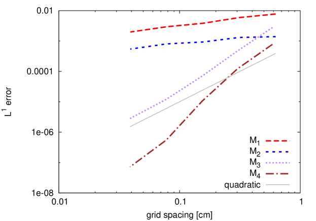
Figure 9: Order of accuracy of the WENO finite difference scheme for the nonlinear advection problem measured in the $L^{1}$ norm. The grey line indicates second-order convergence.

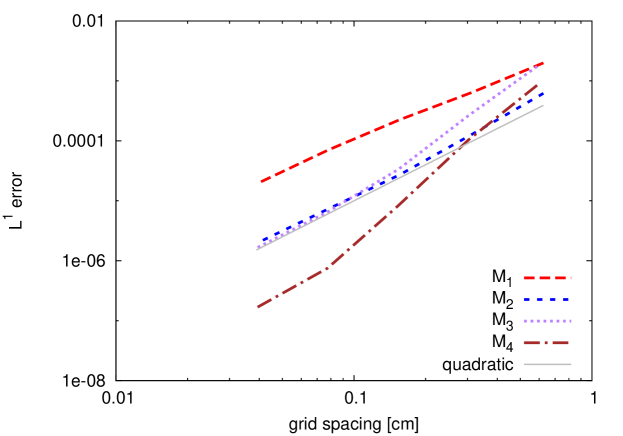
Figure 10: Order of accuracy of the WENO finite volume scheme for the nonlinear advection problem measured in the $L^{1}$ norm. The grey line indicates second-order convergence.

In Figures 9 and 10, the error of the WENO finite difference and the finite volume scheme for the nonlinear advection problem are shown. The error is measured by comparing the numerical solution after $0.2\,{\rm s}$ to the analytical one in the $L^{1}$ norm. We conclude that for the Cartesian and the smooth grid defined by the mapping functions $M_{4}$ and $M_{3}$, both schemes show comparable error sizes. The empirical order of convergence is between two and three for $M_{3}$ and higher than three for $M_{4}$ in both cases.

For the non-smooth mapping functions $M_{1}$ and $M_{2}$, the error does not decrease significantly for the finite difference scheme, whereas first- to second-order convergence can be observed with the finite volume scheme.

grid	$M_{1}$		$M_{2}$		$M_{3}$		$M_{4}$
spacing	error	order	error	order	error	order	error	order
6.25e-1	7.74e-3		1.39e-3		2.77e-3		7.74e-4
3.13e-1	5.89e-3	0.392	1.31e-3	0.088	4.76e-4	2.539	1.23e-4	2.652
1.56e-1	3.83e-3	0.621	9.29e-4	0.492	7.01e-5	2.764	1.05e-5	3.548
7.81e-2	2.95e-3	0.380	8.03e-4	0.209	1.20e-5	2.546	5.46e-7	4.270
3.91e-2	1.98e-3	0.572	5.43e-4	0.566	2.83e-6	2.087	7.21e-8	2.919

Table 1: Mean $L_{1}$ error sizes and order of accuracy for the finite difference scheme.

grid	$M_{1}$		$M_{2}$		$M_{3}$		$M_{4}$
spacing	error	order	error	order	error	order	error	order
6.25e-1	2.00e-3		6.20e-4		1.74e-3		8.46e-4
3.13e-1	6.40e-4	1.643	1.27e-4	2.283	2.64e-4	2.717	1.04e-4	3.018
1.56e-1	2.26e-4	1.498	2.73e-5	2.222	3.37e-5	2.970	8.40e-6	3.635
7.81e-2	7.06e-5	1.681	7.32e-6	1.900	6.53e-6	2.369	7.53e-7	3.480
3.91e-2	1.93e-5	1.869	1.97e-6	1.894	1.63e-6	1.998	1.64e-7	2.201

Table 2: Mean $L_{1}$ error sizes and order of accuracy for the finite volume scheme.

In the finite volume case, we expect second-order convergence for all mappings due to the second-order integration formula used to obtain equation (12). Consequently, we observe second-order convergence for all grids at least asymptotically for high resolution in Table 2. For low resolutions, the numerical solution exhibits third-order convergence indicating that the temporal error dominates in this regime. We note that the Courant number is $0.1$ in all of our tests minimising the error due to the time integration scheme. We conclude that the absolute magnitude of the spatial error strongly depends on the mapping function, whereas the convergence order is restricted by the integration rule used to convert equation (10) into (12). To obtain a higher than second order accurate scheme, high-order integration formulae must be used [35, 34].

On Cartesian grids, the finite difference algorithm is superior compared to the finite volume algorithm. As expected, the scheme is at least third order accurate for all resolutions whereas the finite volume scheme shows second-order convergence for high resolutions. For the smooth mapping $M_{3}$, Visbal and Gaitonde [24] showed that the violation of the freestream preservation leads to large errors which dominate the overall error and decrease the convergence speed. With the non-smooth functions $M_{1}$ and $M_{2}$, this error is particularly large at the diagonals as we can observe for the Gresho vortex in Figure 4. This error does hardly decrease with grid spacing and leads to the slow convergence found in the data from Table 1. We can explain this slow convergence by the fact that in the finite difference approach, the fluxes ${\bf\hat{F}}$ and ${\bf\hat{G}}$ are reconstructed. But these fluxes are non-smooth themselves since they contain the non-smooth metric terms. Therefore, the reconstruction process is only of low order, too.

This test demonstrates once more that the WENO finite difference scheme should only be combined with the mapped grid technique if the mapping function is smooth. With the finite volume scheme, the simulation converges also on non-smooth grids, but at a much slower rate than on smooth grids. With both algorithms, the “smoother” function $M_{2}$ yields more accurate results than $M_{1}$. We conclude that also the finite volume scheme performs better the smoother the grid is. Therefore, non-smooth grids should only be used if absolutely necessary.

For coarse resolutions, the results of $M_{2}$ with the finite volume scheme are better than the results with $M_{1}$, but also with the smooth mapping $M_{3}$. They are even comparable with the Cartesian mapping $M_{4}$. In astrophysical applications where the grid resolution usually is very coarse, grids like the one defined by $M_{2}$ combined with the WENO finite volume algorithm may well yield sufficiently accurate results. These grids are an acceptable alternative, if a non-smooth grid is needed by the problem geometry.

4 Discussion and Outlook

Curvilinear coordinates are an easy and efficient way to extend existing codes written for Cartesian grids to more complicated geometries. The grid can be generated either by a (analytical or numerical) mapping function, or by an external grid generation program. Within the framework introduced in Section 2 it must always be structured.

For the case of spherical domains, Calhoun et al. [1] provided mapping functions which are not strongly differentiable. We showed that the analytical transformation also works in a weak sense without assuming strong differentiability of the mapping function.

In Shu [14], the application of the WENO finite difference scheme to smooth curvilinear grids is shown. The results are of high accuracy, since the mapping functions are smooth and the Mach number of the numerical tests are high.

In this paper, for the first time the WENO finite difference and finite volume scheme were applied with non-smooth mapping functions as those defined by the mapping functions from Calhoun et al. [1]. Particular attention is paid to problems arising when the Mach number of the flow is rather low. Whereas the WENO finite volume scheme performs well in these cases, the WENO finite difference scheme does not give a convergent solution. It only works if the mapping function is smooth, but even in this case the finite volume scheme yields better results for the low Mach number tests presented in this paper.

Since it is only a minor algorithmic change from the WENO finite difference to the WENO finite volume scheme, we recommend to switch to the WENO finite volume scheme when the mapped grid technique is used for non-smooth mapping functions and also for low Mach numbers. As demonstrated in Section 3 the smoother the mapping function is, the more accurate are the results. Therefore, one should always use the smoothest mapping function allowed by the simulation setup.

In theory, the finite volume scheme is only second order accurate. In our calculations, however, the empirical order of accuracy of the finite volume scheme was higher. To increase the theoretical order of accuracy the computational requirements and the complexity of the code has to be increased considerably [34]. In practice, WENO schemes usually are combined with lower order Runge–Kutta methods for time integration with highest-possible Courant numbers. The overall error of the scheme will be dominated by the temporal error, and the overall order of the method will be limited to two or three, anyway.

Furthermore, in astrophysical simulations the typical resolution is rather coarse. In this case the spatial error dominates and fast second order time integrators such as SSP RK(3,2) (Kraaijevanger 28, cf. also Ketcheson et al. 36, Kupka et al. 29) are sufficient. In this regime, non-smooth mapping functions perform nearly as well as smooth ones provided they are combined with the WENO finite volume scheme. We conclude that they are an acceptable alternative, if the problem geometry requires the use of non-smooth mapping functions. Moreover curvilinear coordinates provide enough flexibility for most problems in computational astrophysics whereas keeping the high efficiency and accuracy of the Cartesian schemes they are based on.

We show how the grid capability of an existing code written for Cartesian coordinates can be extended to more general geometries. In this way, a wide variety of astrophysical problems can be tackled with ANTARES which were not feasible with standard grids in numerical astrophysics and without any fundamental changes in the numerical method.

In the near future, we plan to extend our work to the Navier–Stokes equations with gravity and diffusion in three spatial dimensions. It would be interesting to apply low Mach number methods such as the one presented in Kwatra et al. [37] and Happenhofer et al. [10] to curvilinear coordinates and further improve their performance for low Mach numbers.

Furthermore, the influence of the Mach number on the results needs additional investigations. We assume that the distortions due to the freestream preservation violation for finite difference schemes are hidden when there are fast motions of the fluid. Only with low Mach numbers, the numerical errors get large enough to disturb the numerical solution considerably.

Appendix A Finite difference and finite volume discretisation of the Euler equations

First, we derive the finite difference and finite volume discretisation of the Euler equations for the one-dimensional case. The differential form of the Euler equations in one spatial dimension is

$$\frac{\partial}{\partial t}{\bf Q}+\frac{\partial}{\partial x}{\bf F}=0,$$ (27)

$${\bf Q}=\left(\begin{array}[]{c}\rho\\ \rho u\\ E\end{array}\right),\ {\bf F}\left({\bf Q}\right)=\left(\begin{array}[]{c}\rho u\\ \rho u^{2}+p\\ (p+E)u\end{array}\right),$$ (28)

where $p=p(\rho,e)$. The internal energy $e$ is given by $e=E-\frac{u^{2}}{2\rho}$. Let $\Omega=\left[a,b\right]$ and let a grid on $\Omega$ be defined on the half-integer nodes, i.e.

$$x_{i+\frac{1}{2}}=x_{i-\frac{1}{2}}+\delta x_{i},\ i=1,\ldots,n,\ x_{\frac{1}{2}}=a,x_{n+\frac{1}{2}}=b.$$ (29)

The grid is not necessarily equidistant. The index $i$ refers to the centre of the cell $C_{i}=\left[x_{i-\frac{1}{2}},x_{i+\frac{1}{2}}\right]$.

Definition 1.

The Cell Average Operator $\mathrm{A}$ on a grid (29) is defined by

$$\mathrm{A}(h)_{i}:=\frac{1}{\delta x_{i}}\int_{x_{i-\frac{1}{2}}}^{x_{i+\frac{1}{2}}}h(\hat{x})d\hat{x}.$$ (30)

Applying $\mathrm{A}$ to (27) gives

$$\frac{\partial}{\partial t}\left(\mathrm{A}{\bf Q}\right)_{i}+\frac{\delta{\bf F}_{i}}{\delta x_{i}}=0\text{ with }\frac{\delta{\bf F}_{i}}{\delta x_{i}}=\frac{{\bf F}_{i+\frac{1}{2}}-{\bf F}_{i-\frac{1}{2}}}{\delta x_{i}}$$ (31)

with ${\bf F}_{i+\frac{1}{2}}={\bf F}\left({\bf Q}(x_{i+\frac{1}{2}})\right)$. $\left(\mathrm{A}{\bf Q}\right)_{i}=:\overline{{\bf Q}}_{i}$ is the Cell Average of ${\bf Q}$ in the cell $C_{i}=\left[x_{i-\frac{1}{2}},x_{i+\frac{1}{2}}\right]$.

Applying now $\mathrm{A}^{-1}$ as in Merriman [15], we get

$$\frac{\partial}{\partial t}{\bf Q}_{i}+\mathrm{A}^{-1}\frac{\delta{\bf F}_{i}}{\delta x_{i}}=0.$$ (32)

Merriman [15] showed that

$$\mathrm{A}^{-1}\frac{\delta{\bf F}_{i}}{\delta x_{i}}=\frac{\delta\left(\mathrm{A}^{-1}{\bf F}_{i}\right)}{\delta x_{i}}\text{ if the grid is equidistant, i.e. }\delta x_{i}=\delta x\ \forall i.$$ (33)

In general, this is not the case since $\frac{\delta{\bf F}_{i}}{\delta x_{i}}$ is a translation operator, but $\mathrm{A}$ is not translation-invariant. For an equidistant grid, however, (32) is equivalent to

$$\frac{\partial}{\partial t}{\bf Q}_{i}+\frac{\delta{\bf f}_{i}}{\delta x_{i}}=0\text{ with }{\bf F}_{i}=(\mathrm{A}{\bf f})_{i}.$$ (34)

(34) is called the Shu–Osher form of (27). It is equivalent to (1) if the grid is equidistant [15]. ${\bf f}$ is defined such that its average in cell $C_{i}$ is given by the point value of the analytical flux function ${\bf F}$ at the cell centre. In terms of Shu and Osher [13], ${\bf F}$ is exactly the “primitive function” of ${\bf f}$.

A finite volume scheme starts with equation (31) and computes approximations for ${\bf Q}_{i+\frac{1}{2}}$ from the given cell averaged $\overline{{\bf Q}}_{i}$. The numerical flux ${\bf F}_{i+\frac{1}{2}}$ is calculated by

$${\bf F}_{i+\frac{1}{2}}={\bf F}\left({\bf Q}_{i+\frac{1}{2}}\right).$$ (35)

In contrast, the finite difference scheme starts with equation (34) and computes approximations for ${\bf f}_{i+\frac{1}{2}}$ from the values of the analytical flux function ${\bf F}$. Since ${\bf F}_{i}=(\mathrm{A}{\bf f})_{i}$, both approaches are computationally equivalent and require the numerical solution of the following

Problem 2 (Reconstruction problem).

Given a set of cell averages, compute the value of the underlying function at the half-integer nodes.

Definition 2.

The Reconstruction Operator $\mathrm{R}$ acts on cell averages and reconstructs the point value of the underlying function

$$\mathrm{R}(\mathrm{A}h)_{i+\frac{1}{2}}=h_{i+\frac{1}{2}}$$ (36)

on a given grid (29).

If the grid is equidistant, the same algorithm can be used to compute ${\bf Q}_{i+\frac{1}{2}}$ and ${\bf f}_{i+\frac{1}{2}}$. The only difference lies in the input for the reconstruction process: in the case of a finite volume scheme, the inputs are given by the cell averages $\overline{\bf Q}_{i}$ of the state vector, whereas in the case of a finite difference scheme, they are given by the analytical flux function ${\bf F}$ evaluated at the cell centre.

Given a reconstruction operator $\mathrm{R}$, Problem 2 can be solved. The WENO reconstruction operator is described in detail in Shu [14] and also in C, following the cited reference. In general, finite volume methods can be designed on non-equidistant grids. However, since the WENO reconstruction operator as it is described in C works only on equidistant grids, the applicability of the finite volume method using this reconstruction method is restricted to equidistant grids, too.

The advantage of the finite difference scheme lies in its easy extension to higher dimensions. Let a region (i.e., a non-empty, open, and connected set) $\Omega\subset\mathbb{R}^{2}$ be given. The Euler equations are a system of partial differential equations on $\Omega$. In two spatial dimensions and in a Cartesian coordinate system, their differential form is

$$\frac{\partial}{\partial t}{\bf Q}+\frac{\partial}{\partial x}{\bf F}+\frac{\partial}{\partial y}{\bf G}=0,$$ (37)

with the state vector ${\bf Q}$ and the flux functions ${\bf F}$ and ${\bf G}$ given by

$${\bf Q}=\left(\begin{array}[]{c}\rho\\ \rho u\\ \rho v\\ E\end{array}\right),{\bf F}\left({\bf Q}\right)=\left(\begin{array}[]{c}\rho u\\ \rho u^{2}+p\\ \rho uv\\ (p+E)u\end{array}\right),{\bf G}\left({\bf Q}\right)=\left(\begin{array}[]{c}\rho v\\ \rho vu\\ \rho v^{2}+p\\ (p+E)v\end{array}\right),$$ (38)

where $p=p(\rho,e)$. In the following, we will write ${\bf u}:=\left(u,v\right)^{T}$ for the velocity vector.

In the finite volume approach, applying $\mathrm{A}_{x}\mathrm{A}_{y}$ to the two-dimensional Euler equations (1) results in

$$\frac{\partial}{\partial t}\left(\mathrm{A}_{x}\mathrm{A}_{y}{\bf Q}\right)_{i,j}+\frac{\mathrm{A}_{y}({\bf F}_{i+\frac{1}{2}})_{j}-\mathrm{A}_{y}({\bf F}_{i-\frac{1}{2}})_{j}}{\delta x}+\frac{\mathrm{A}_{x}({\bf G}_{j+\frac{1}{2}})_{i}-\mathrm{A}_{x}({\bf G}_{j-\frac{1}{2}})_{i}}{\delta y}=0.$$ (39)

The fluxes are now line integrals over the cell boundaries. With the midpoint rule,

$$\mathrm{A}_{y}({\bf F}_{i+\frac{1}{2}})_{j}={\bf F}_{i+\frac{1}{2},j}+O(h^{2}).$$ (40)

With only one evaluation of the fluxes, the overall order of the method is restricted to two. We remark that if ${\bf F}$ is linear, this integration is exact.

Contrary, in the finite difference approach, (37) is transformed to

$$\frac{\partial}{\partial t}{\bf Q}_{i,j}+\frac{{\bf f}_{i+\frac{1}{2},j}-{\bf f}_{i-\frac{1}{2},j}}{\delta x}+\frac{{\bf g}_{i,j+\frac{1}{2}}-{\bf g}_{i,j-\frac{1}{2}}}{\delta y}=0$$ (41)

with ${\bf F}=\mathrm{A}_{x}({\bf f})$ and ${\bf G}=\mathrm{A}_{y}({\bf g})$. The overall order of the method only depends on the order of the reconstruction of ${\bf f}$ and ${\bf g}$, which are one-dimensional reconstruction problems. The one-dimensional algorithms can be directly applied without loss of order of accuracy.

Even if the high order one-dimensional WENO reconstruction algorithm is applied to evaluate the flux functions in (39), the resulting finite volume method is only second order accurate. To obtain a truely high-order multidimensional finite volume method, more complicated integrations for the line integrals in (39) must be performed, increasing the computational costs of the finite volume scheme tremendously [14, 26, 34]. Therefore, finite difference schemes are clearly preferable on Cartesian grids.

Appendix B Classical Transformation to Curvilinear Coordinates Assuming Strong Differentiability

If there is a differentiable function

$$M:\ \left[-1,1\right]^{2}\to\Omega,\ M(\xi,\eta)=(x,y)^{T},$$ (42)

we can transform the Euler equations in differential form (1) to

$$\frac{\partial}{\partial t}J^{-1}{\bf Q}+\frac{\partial}{\partial\xi}{\bf\hat{F}}+\frac{\partial}{\partial\eta}{\bf\hat{G}}=0$$ (43a)

with

$${\bf\hat{F}}= \frac{\partial y}{\partial\eta}{\bf F}-\frac{\partial x}{\partial\eta}{\bf G},$$ (43b)

$${\bf\hat{G}}= -\frac{\partial y}{\partial\xi}{\bf F}+\frac{\partial x}{\partial\xi}{\bf G},$$ (43c)

and the determinant of the inverse Jacobian of the transformation

$$J^{-1}=\left|\frac{\partial(x,y)}{\partial(\xi,\eta)}\right|=\frac{\partial y}{\partial\eta}\frac{\partial x}{\partial\xi}-\frac{\partial y}{\partial\xi}\frac{\partial x}{\partial\eta}.$$ (43d)

In this way, the conservation law (1) defined in the physical space is transformed into a conservation law in the computational space. If $M$ is at least in $C^{1}$, all derivatives and the Jacobian are well-defined [38, 20].

Following the description in Tannehill et al. [39], this form can be derived by multiplying (1) with $J^{-1}$ and rearranging terms. First we look at $\frac{\partial{\bf F}}{\partial x}J^{-1}$. With the chain rule of differentiation,

$$\frac{\partial\bf F}{\partial x}J^{-1} =\left(\frac{\partial\xi}{\partial x}\frac{\partial\bf F}{\partial\xi}+\frac{\partial\eta}{\partial x}\frac{\partial\bf F}{\partial\eta}\right)J^{-1}$$

$$=\frac{\partial}{\partial\xi}\left({\bf F}\frac{\partial\xi}{\partial x}J^{-1}\right)+\frac{\partial}{\partial\eta}\left({\bf F}\frac{\partial\eta}{\partial x}J^{-1}\right)$$

$$-{\bf F}\frac{\partial}{\partial\xi}\left(\frac{\partial\xi}{\partial x}J^{-1}\right)-{\bf F}\frac{\partial}{\partial\eta}\left(\frac{\partial\eta}{\partial x}J^{-1}\right).$$

In two dimensions,

$$\left(\begin{array}[]{cc}\frac{\partial\xi}{\partial x}&\frac{\partial\xi}{\partial y}\\ \frac{\partial\eta}{\partial x}&\frac{\partial\eta}{\partial y}\end{array}\right)=\left(\begin{array}[]{cc}\frac{\partial x}{\partial\xi}&\frac{\partial x}{\partial\eta}\\ \frac{\partial y}{\partial\xi}&\frac{\partial y}{\partial\eta}\end{array}\right)^{-1}=J\left(\begin{array}[]{cc}\frac{\partial y}{\partial\eta}&-\frac{\partial x}{\partial\eta}\\ -\frac{\partial y}{\partial\xi}&\frac{\partial x}{\partial\xi}\end{array}\right),$$ (44)

and as a direct consequence,

$$\frac{\partial\xi}{\partial x}J^{-1}=\frac{\partial y}{\partial\eta},\ \frac{\partial\xi}{\partial y}J^{-1}=-\frac{\partial x}{\partial\eta},\ \frac{\partial\eta}{\partial x}J^{-1}=-\frac{\partial y}{\partial\xi},\ \frac{\partial\eta}{\partial y}J^{-1}=\frac{\partial x}{\partial\xi}.$$ (45)

We can further write

$$\frac{\partial\bf F}{\partial x}J^{-1} =\frac{\partial}{\partial\xi}\left(\frac{\partial y}{\partial\eta}{\bf F}\right)+\frac{\partial}{\partial\eta}\left(-\frac{\partial y}{\partial\xi}{\bf F}\right)-{\bf F}\underbrace{\left(\frac{\partial^{2}y}{\partial\xi\partial\eta}-\frac{\partial^{2}y}{\partial\eta\partial\xi}\right)}_{=0}.$$

Here we assumed the mapping function to be at least in $C^{2}$. The same procedure leads to similar expressions for $\frac{\partial{\bf G}}{\partial y}J^{-1}$. Plugging all these expressions into (1) leads to (43d).

Appendix C The $5$th order WENO Reconstruction Algorithm

In the following, the WENO reconstruction operator is derived following Shu [14]. The purpose of the reconstruction operator is to solve Problem 2, i.e. reconstruct the value of the underlying function at a certain position given a set of cell averages.

We will only consider equidistant one-dimensional grids and reconstruction of the value at the half-integer node $i+\frac{1}{2}$. This is sufficient for the finite difference and finite volume algorithms used in this paper.

The idea of the WENO reconstruction process is to use several stencils in the neighbourhood of $i+\frac{1}{2}$. On each of the stencils, an interpolating polynomial of high order is defined. The interpolated value is obtained by summing these polynomials weighting them according to their smoothness. If a discontinuity is contained in the stencil of a polynomial, its weight will be very small thereby avoiding oscillatory behaviour known from high order interpolation.

Assume that the cell averages $\overline{\phi}_{i}=(\mathrm{A}\phi)_{i}$ of the function $\phi$ are given and $\phi_{i+\frac{1}{2}}$ should be reconstructed. We consider $k$ stencils

$$S_{r}(i)=\{x_{i-r},\ldots,x_{i-r+k-1}\},\ r=0,\ldots,k-1.$$ (46)

On each stencil $S_{r}(i)$ a polynomial $p_{r}$ of degree $k-1$ is defined such that the approximation $\phi_{i+\frac{1}{2}}^{(r)}$ to $\phi_{i+\frac{1}{2}}$ is given by

$$\phi_{i+\frac{1}{2}}^{(r)}=p_{r}(x_{i+\frac{1}{2}})+O((\delta x)^{k})$$ (47)

and

$$\mathrm{A}(p_{r})=\mathrm{A}(\phi)=\overline{\phi}\text{ on }S_{r}(i).$$ (48)

Solving the resulting linear system for the case $k=3$ gives the interpolation polynomials

$$p_{0}(x_{i+\frac{1}{2}}) =\frac{1}{3}\overline{\phi}_{i-2}-\frac{7}{6}\overline{\phi}_{i-1}+\frac{11}{6}\overline{\phi}_{i},$$ (49)

$$p_{1}(x_{i+\frac{1}{2}}) =-\frac{1}{6}\overline{\phi}_{i-1}+\frac{5}{6}\overline{\phi}_{i}+\frac{1}{3}\overline{\phi}_{i+1},$$ (50)

$$p_{2}(x_{i+\frac{1}{2}}) =\frac{1}{3}\overline{\phi}_{i}+\frac{5}{6}\overline{\phi}_{i+1}-\frac{1}{6}\overline{\phi}_{i+2},$$ (51)

The Lagrange polynomial of fifth order can be obtained by combination of the three polynomials of third order. If we define the weights

$$d_{0}=\frac{3}{10},d_{1}=\frac{3}{5},d_{2}=\frac{1}{10},$$ (52)

the fifth order interpolation polynomial $p^{(5)}$ can be obtained by

$$p^{(5)}(x)=d_{0}p_{0}(x)+d_{1}p_{1}(x)+d_{2}p_{2}(x).$$ (53)

High-order polynomial interpolation is known to produce oscillatory results. To avoid oscillations in the WENO approach, a convex combination of all candidate stencils $p_{r}$ is used to compute $\phi_{i+\frac{1}{2}}$. This procedure leads to non-oscillatory approximations of order $2k-1$, where $k$ is the width of each of the stencils $S_{r}(i)$.

Therefore, the approximation to $\phi_{i+\frac{1}{2}}$ is calculated by

$$\phi_{i+\frac{1}{2}}=\omega_{0}p_{0}(x_{i+\frac{1}{2}})+\omega_{1}p_{1}(x_{i+\frac{1}{2}})+\omega_{2}p_{2}(x_{i+\frac{1}{2}}),$$ (54)

where $\omega_{0}$, $\omega_{1}$ and $\omega_{2}$ are nonlinear weights comparing the smoothness of the interpolation polynomials. Defining

$$\begin{split}\beta_{0}&=\frac{13}{12}\left(\overline{\phi}_{i}-\overline{\phi}_{i+1}+\overline{\phi}_{i+2}\right)^{2}+\frac{1}{4}\left(3\overline{\phi}_{i}-4\overline{\phi}_{i+1}+\overline{\phi}_{i+2}\right)^{2},\\ \beta_{1}&=\frac{13}{12}\left(\overline{\phi}_{i-1}-2\overline{\phi}_{i}+\overline{\phi}_{i+1}\right)^{2}+\frac{1}{4}\left(\overline{\phi}_{i-1}-\overline{\phi}_{i+1}\right)^{2},\\ \beta_{2}&=\frac{13}{12}\left(\overline{\phi}_{i-2}-2\overline{\phi}_{i-1}+\overline{\phi}_{i}\right)^{2}+\frac{1}{4}\left(\overline{\phi}_{i-2}-4\overline{\phi}_{i-1}\right)^{2},\end{split}$$ (55)

we calculate

$${\tilde{\omega}}_{0}=\frac{d_{0}}{(\beta_{0}+\epsilon)^{2}},\ {\tilde{\omega}}_{1}=\frac{d_{1}}{(\beta_{1}+\epsilon)^{2}},\ {\tilde{\omega}}_{2}=\frac{d_{2}}{(\beta_{2}+\epsilon)^{2}},$$ (56)

and finally

$$\omega_{0}=\frac{{\tilde{\omega}}_{0}}{{\tilde{\omega}}_{0}+{\tilde{\omega}}_{1}+{\tilde{\omega}}_{2}},\ \omega_{1}=\frac{{\tilde{\omega}}_{1}}{{\tilde{\omega}}_{0}+{\tilde{\omega}}_{1}+{\tilde{\omega}}_{2}},\ \omega_{2}=\frac{{\tilde{\omega}}_{2}}{{\tilde{\omega}}_{0}+{\tilde{\omega}}_{1}+{\tilde{\omega}}_{2}}.$$ (57)

$\epsilon$ is a small parameter which is used to avoid division by zero.

References

- Calhoun et al. [2008] D. A. Calhoun, C. Helzel, R. J. LeVeque, Logically Rectangular Grids and Finite Volume Methods for PDEs in Circular and Spherical Domains, SIAM Review 50 (2008) 723 – 752.
- Browning et al. [2004] M. K. Browning, A. S. Brun, J. Toomre, Simulations Of Core Convection In Rotating A-type Stars: Differential Rotation And Overshooting, ApJ 601 (2004) 512 – 529.
- Cai et al. [2011] T. Cai, K. L. Chan, L. Deng, Numerical simulation of core convection by a multi-layer semi-implicit spherical spectral method, JCP 230 (2011) 8698 – 8712.
- Evonuk and Glatzmaier [2006] M. Evonuk, G. A. Glatzmaier, 2D study of the effects of the size of a solid core on the equatorial flow in giant planets, Icarus 181 (2006) 458 – 464.
- Evonuk and Glatzmaier [2007] M. Evonuk, G. A. Glatzmaier, The effects of rotation rate on deep convection in giant planets with small solid cores, Planetary and Space Science 55 (2007) 407 – 412.
- Freytag et al. [2002] B. Freytag, M. Steffen, B. Dorch, Spots on the surface of Betelgeuse — Results from new 3D stellar convection models, Astron. Nachr. 323 (2002) 213 – 219.
- Zingale et al. [2013] M. Zingale, A. Nonaka, A. S. Almgren, J. B. Bell, C. M. Malone, R. Orvedahl, Low Mach Number Modeling of Convection in Helium Shells on Sub-Chandrasekhar White Dwarfs. I. Methodology, ApJ 764 (2013) 97 – 110.
- Mocz et al. [2013] P. Mocz, M. Vogelsberger, D. Sijacki, R. Pakmor, L. Hernquist, A discontinuous Galerkin method for solving the fluid and MHD equations in astrophysical simulations, MNRAS (2013). Available at http://arxiv.org/abs/1305.5536.
- Muthsam et al. [2010] H. J. Muthsam, F. Kupka, B. Löw-Baselli, C. Obertscheider, M. Langer, P. Lenz, ANTARES – A Numerical Tool for Astrophysical RESearch with applications to solar granulation, NewA 15 (2010) 460 – 475.
- Happenhofer et al. [2013] N. Happenhofer, H. Grimm-Strele, F. Kupka, B. Löw-Baselli, H. J. Muthsam, A low Mach number solver: Enhancing applicability, JCP 236 (2013) 96 – 118.
- Muthsam et al. [2010] H. J. Muthsam, F. Kupka, E. Mundprecht, F. Zaussinger, H. Grimm-Strele, N. Happenhofer, Simulations of stellar convection, pulsation and semiconvection, in: N. Brummell, A. Brun, M. Miesch, Y. Ponty (Eds.), Astrophysical Dynamics: From Stars to Galaxies, number 271 in Proceedings IAU Symposium, pp. 179 – 186.
- Mundprecht et al. [2013] E. Mundprecht, H. J. Muthsam, F. Kupka, Multidimensional realistic modelling of Cepheid-like variables. I. Extensions of the ANTARES code, MNRAS 435 (2013) 3191 – 3205.
- Shu and Osher [1988] C.-W. Shu, S. Osher, Efficient implementation of essentially non-oscillatory shock-capturing schemes, JCP 77 (1988) 439 – 471.
- Shu [2003] C.-W. Shu, High-order Finite Difference and Finite Volume WENO Schemes and Discontinuous Galerkin Methods for CFD, International Journal of Computational Fluid Dynamics 17 (2003) 107 – 118.
- Merriman [2003] B. Merriman, Understanding the Shu–Osher Conservative Finite Difference Form, Journal Of Scientific Computing 19 (2003) 309 – 322.
- Muthsam et al. [2007] H. J. Muthsam, B. Löw-Baselli, C. Obertscheider, M. Langer, P. Lenz, F. Kupka, High–resolution models of solar granulation: the two–dimensional case, MNRAS 380 (2007) 1335 – 1340.
- Wesseling [2001] P. Wesseling, Principles of Computational Fluid Dynamics, volume 29 of Springer Series in Computational Mathematics, Springer, Berlin Heidelberg New–York, 2001.
- Ferziger and Perić [2002] J. H. Ferziger, M. Perić, Computational Methods for Fluid Dynamics, Springer, Berlin, 3rd edition, 2002.
- LeVeque [2004] R. J. LeVeque, Finite–Volume Methods for Hyperbolic Problems, Cambridge Texts in Applied Mathematics, Cambridge University Press, 2004.
- Kifonidis and Müller [2012] K. Kifonidis, E. Müller, On multigrid solution of the implicit equations of hydrodynamics. Experiments for the compressible Euler equations in general coordinates, A&A 544 (2012) A47.
- Thompson et al. [1985] J. F. Thompson, Z. U. A. Warsi, C. Wayne Mastin, Numerical Grid Generation. Foundations and Applications, North–Holland, 1985.
- Evans [2002] L. C. Evans, Partial Differential Equations, volume 19 of Graduate Studies in Mathematics, American Mathematical Society, 2nd edition, 2002.
- Chorin and Marsden [1993] A. J. Chorin, J. E. Marsden, A Mathematical Introduction to Fluid Mechanics, volume 4 of Texts in Applied Mathematics, Springer, New–York Berlin Heidelberg, 3rd edition, 1993.
- Visbal and Gaitonde [2002] M. R. Visbal, D. V. Gaitonde, On the Use of Higher-Order Finite-Difference Schemes on Curvilinear and Deforming Meshes, JCP 181 (2002) 155 – 185.
- Nonomura et al. [2010] T. Nonomura, N. Iizuka, K. Fujii, Freestream and vortex preservation properties of high-order WENO and WCNS on curvilinear grids, Computers & Fluids 39 (2010) 197 – 214.
- Colella et al. [2011] P. Colella, M. R. Dorr, J. A. F. Hittinger, D. F. Martin, High-order, finite-volume methods in mapped coordinates, JCP 230 (2011) 2952 – 2976.
- Donat and Marquina [1996] R. Donat, A. Marquina, Capturing Shock Reflections: An Improved Flux Formula, JCP 125 (1996) 42 – 58.
- Kraaijevanger [1991] J. F. B. M. Kraaijevanger, Contractivity of Runge-Kutta methods, BIT 31 (1991) 482 – 528.
- Kupka et al. [2012] F. Kupka, N. Happenhofer, I. Higueras, O. Koch, Total-variation-diminishing implicit–explicit Runge–Kutta methods for the simulation of double-diffusive convection in astrophysics, JCP 231 (2012) 3561 – 3586.
- Miczek [2013] F. Miczek, Simulation of low Mach number astrophysical flows, Ph.D. thesis, TU München, 2013.
- Liska and Wendroff [2003] R. Liska, B. Wendroff, Comparions of Several Difference Schemes on 1D and 2D Test Problems for the Euler Equations, SIAM Journal on Scientific Computing 25 (2003) 1 – 30. Available at http://www-troja.fjfi.cvut.cz/~liska/CompareEuler/compare8/.
- Sod [1978] G. A. Sod, A survey of several finite difference methods for systems of nonlinear hyperbolic conservation laws, JCP 27 (1978) 1 – 31.
- Yee et al. [1999] H. Yee, N. Sandham, M. Djomehri, Low-Dissipative High-Order Shock-Capturing Methods Using Characteristic-Based Filters, JCP 150 (1999) 199 – 238.
- Zhang et al. [2011] R. Zhang, M. Zhang, C.-W. Shu, On the Order of Accuracy and Numerical Performance of Two Classes of Finite Volume WENO Schemes, Commun. Comput. Phys. 9 (2011) 807 – 827.
- Casper and Atkins [1993] J. Casper, H. L. Atkins, A Finite-Volume High-Order ENO Scheme for Two-Dimensional Hyperbolic Systems, JCP 106 (1993) 62 – 76.
- Ketcheson et al. [2009] D. I. Ketcheson, C. B. Macdonald, S. Gottlieb, Optimal implicit strong stability preserving Runge–Kutta methods, Applied Numerical Mathematics 59 (2009) 373 – 392.
- Kwatra et al. [2009] N. Kwatra, J. Su, J. T. Gretarsson, R. Fedkiw, A method for avoiding the acoustic time step restriction in compressible flow, JCP 228 (2009) 4146 – 4161.
- Vinokur [1974] M. Vinokur, Conservation Equations of Gasdynamics in Curvilinear Coordinate Systems, JCP 14 (1974) 105 – 125.
- Tannehill et al. [1997] J. C. Tannehill, D. A. Anderson, R. H. Pletcher, Computational Fluid Mechanics and Heat Transfer, Taylor & Francis, 1997.