Reactivity Boundaries to Separate the Fate of a Chemical Reaction Associated with Multiple Saddles

Abstract

Reactivity boundaries that divide the origin and destination of trajectories are crucial of importance to reveal the mechanism of reactions, which was recently found to exist robustly even at high energies for index-one saddles [Phys. Rev. Lett. 105, 048304 (2010)]. Here we revisit the concept of the reactivity boundary and propose a more general definition that can involve a single reaction associated with a bottleneck made up of higher index saddles and/or several saddle points with different indices, where the normal form theory, based on expansion around a single stationary point, does not work. We numerically demonstrate the reactivity boundary by using a reduced model system of the $\mathrm{H}_{5}^{+}$ cation where the proton exchange reaction takes place through a bottleneck made up of two index-two saddle points and two index-one saddle points. The cross section of the reactivity boundary in the reactant region of the phase space reveals which initial conditions are effective in making the reaction happen, and thus sheds light on the reaction mechanism.

I Introduction

Studies of chemical reaction dynamics aims for understanding of how and why a system proceeds from its initial state to the final state in the process of reaction. Special interest lies in the question of what initial conditions make the reaction happen. Classically, the process of chemical reaction can be regarded as motion of a point in the phase space propagating from a region corresponding to the reactant to another region corresponding to the product. Some phase space points in the reactant region may go into the product region after time propagation, whereas other phase space points stay in the reactant region without undergoing the reaction. In between these reactive initial conditions and non-reactive ones lies a boundary which we simply call here reactivity boundary  that was previously described by various words, such as “boundary trajectories” Pechukas (1976); Pechukas and Pollak (1977); Sverdlik and Koeppl (1978); Pollak and Pechukas (1978); Pechukas and Pollak (1979); Pollak and Pechukas (1979); Child and Pollak (1980); Pollak et al. (1980); Pollak and Levine (1980); Pollak and Child (1980); Pechukas (1981); Pollak (1981a, b, c) asymptotic to periodic orbit dividing surface (pods) Child and Pollak (1980); Pollak et al. (1980); Pollak and Levine (1980); Pollak and Child (1980); Pechukas (1981); Pollak (1981a, b, c), “boundary of” Pechukas (1976); Pechukas and Pollak (1977); Sverdlik and Koeppl (1978); Pollak and Pechukas (1978); Pechukas and Pollak (1979); Pollak and Pechukas (1979); Child and Pollak (1980); Pollak et al. (1980); Pollak and Levine (1980); Pollak and Child (1980); Pechukas (1981); Pollak (1981a, b, c) reactivity bandsWall et al. (1958, 1961); Wall and Porter (1963); Wright et al. (1975); Wright (1976); Wright and Tan (1977); Laidler et al. (1977); Tan et al. (1977); Wright (1978); Andrews and Chesnavich (1984); Grice et al. (1987), “tube”de Almeida et al. (1990), “cylindrical manifold”de Almeida et al. (1990), “impenetrable barriers”Wiggins et al. (2001), “stable/unstable manifold” of normally hyperbolic invariant manifolds (NHIM)Wiggins et al. (2001), “reaction boundaries”Kawai and Komatsuzaki (2010), and also described on certain sections, such as “reactivity bands”Wall et al. (1958, 1961); Wall and Porter (1963); Wright et al. (1975); Wright (1976); Wright and Tan (1977); Laidler et al. (1977); Tan et al. (1977); Wright (1978); Andrews and Chesnavich (1984); Grice et al. (1987), “reactivity map” Wright et al. (1975); Wright (1976); Wright and Tan (1977); Laidler et al. (1977); Tan et al. (1977); Wright (1978); Andrews and Chesnavich (1984); Grice et al. (1987), “reactive island”de Almeida et al. (1990). The general definition of the reactivity boundary is the main subject of this paper.

The reactivity boundary is often discussed in relation to saddle points. A saddle point on a multi-dimensional potential energy surface is defined as a stationary point at which the Hessian matrix does not have zero eigenvalues and, at least, one of the eigenvalues is negative. Saddle points are classified by the number of the negative eigenvalues and a saddle that has $n$ negative eigenvalues is called an index-$n$ saddle. Especially the index-one saddle on a potential surface has long been considered to make bottleneck of reactionsGlasstone et al. (1941); Steinfeld et al. (1989), with the sole unstable direction corresponding to the “reaction coordinate.” This is because index-one saddle is considered to be the lowest energy stationary point connecting two potential minima, of which one corresponds to the reactant and the other to the product, and the system must traverse the vicinity of the index-one saddle from the reactant to the product Zhang et al. (2006); Skodje et al. (2000); Shiu et al. (2004).

Such reactivity boundaries have been investigated from early period of the study of reaction dynamics. Especially reactivity boundaries of atom-diatom reactions were extensively studied by Wright et al.Wright et al. (1975); Wright (1976); Wright and Tan (1977); Tan et al. (1977); Wright (1978); Laidler et al. (1977) and Pechukas et al.Pollak and Levine (1980); Pollak (1981c, a); Pechukas (1976); Sverdlik and Koeppl (1978); Pollak and Pechukas (1979); Pollak and Child (1980); Child and Pollak (1980); Pollak and Pechukas (1978); Pollak (1981b); Pollak et al. (1980); Pechukas and Pollak (1979, 1977); Pechukas (1981). At very early period, Wigner introduced asymptotic reactant and product regions to calculate reaction rate in the line of his achievement of the transition state theoryWigner (1937). Independently, Wright et al. showed reactive bands, which had been found by Wall et al.Wall et al. (1961); Wall and Porter (1963); Wall et al. (1958), in the reactivity maps of $\mathrm{H}+\mathrm{H}_{2}$ and its isotopic variantsWright et al. (1975); Wright (1976); Wright and Tan (1977); Tan et al. (1977); Wright (1978); Laidler et al. (1977) that consist of bands of nonreactive regions and reactive regions of each product. The approach was initiated by Ref. Wright et al., 1975 to see the origin of continuous shift of peak in graph of initial relative translational (kinetic) energy versus time spent in “reaction shell” for given initial vibrational phase angles. After Ref. Wright et al., 1975, a series of study was reported for collinear (1D)Wright (1976), isotopeWright and Tan (1977), coplanar (2D)Tan et al. (1977) reactions and 3DWright (1978) reaction and also on an improved potential energy surfaceLaidler et al. (1977) with the plot of initial relative translational energy versus initial phase angle $\theta$. Chesnavich et al. observed boundary trajectories of the collision-induced dissociation of $\mathrm{H}+\mathrm{H}_{2}$ reactionAndrews and Chesnavich (1984); Grice et al. (1987) that divide reactive ($\mathrm{H}_{2}+\mathrm{H}$), non-reactive ($\mathrm{H}+\mathrm{H}_{2}$) and dissociative ($\mathrm{H}+\mathrm{H}+\mathrm{H}$) regions in phase space.

Pechukas et al. revealed the role of periodic orbit dividing surface in two-dimensional collinear atom-diatom reaction systems Pollak and Levine (1980); Pollak (1981c, a); Pechukas (1976); Sverdlik and Koeppl (1978); Pollak and Pechukas (1979); Pollak and Child (1980); Child and Pollak (1980); Pollak and Pechukas (1978); Pollak (1981b); Pollak et al. (1980); Pechukas and Pollak (1979, 1977); Pechukas (1981). The importance of periodic orbit around interaction region was first recognized by PechukasPechukas (1976). The series of research can be described by his words at very beginning.

Somewhere between these two trajectories is a “dividing” trajectory that falls away, neither to reactant nor to product; this is the required “vibration,” across the saddle point region but not necessarily through the saddle point, and the curve executed on the plane by the vibration is the best transition state at that energy.

Pechukas and PollakPechukas and Pollak (1977) and Sverdlik and KoepplSverdlik and Koeppl (1978) started to observe such trajectories in the region of index-one saddles of two dimensional systems and recognized as “unstable invariant classical manifold”Pechukas (1981) and call them periodic orbit dividing surface (pods)Pollak et al. (1980). The pods can be identified as the best transition statePechukas and Pollak (1979) when there is only one pods at given energy. Pechukas and Pollak investigated the advantage of pods against variational TSTPollak and Pechukas (1978) and unified statistical theoryPollak and Pechukas (1979). They also revealed its role in the application of statistical theories to reaction dynamicsPollak and Pechukas (1979); Pollak and Levine (1980); Child and Pollak (1980) and provided an iterative method to calculate reaction probabilityPollak and Child (1980). After the series of classical investigation they started to look at adiabatic motion perpendicular to podsPollak (1981b) and quantum correspondencePollak (1981a) and experimental correspondencePollak (1981c) were elucidated. Those studies were mostly done on two degrees of freedom (DoFs) systems. The problem one of high dimension in the region of index-one saddles was later overcome Komatsuzaki and Nagaoka (1996, 1997); Komatsuzaki and Berry (1999, 2001); Wiggins et al. (2001); Uzer et al. (2002); Bartsch et al. (2005); Li et al. (2006); Kawai and Komatsuzaki (2010); Hernandez et al. (2010); Kawai and Komatsuzaki (2011a); Waalkens et al. (2008); Kawai and Komatsuzaki (2011b, c); Ünver Çiftçi and Waalkens (2012); Teramoto et al. (2011); Toda et al. (2005); Komatsuzaki et al. (2011); Jaffé et al. (2005); Martens (2002); Komatsuzaki and Berry (2003); de Almeida et al. (1990).

The dynamics around the saddle point is recently investigated extensively in terms of nonlinear dynamics Komatsuzaki and Berry (1999, 2001); Wiggins et al. (2001); Uzer et al. (2002); Bartsch et al. (2005); Li et al. (2006); Kawai and Komatsuzaki (2010); Hernandez et al. (2010); Kawai and Komatsuzaki (2011a); Waalkens et al. (2008); Kawai and Komatsuzaki (2011b, c); Ünver Çiftçi and Waalkens (2012); Teramoto et al. (2011); Toda et al. (2005); Komatsuzaki et al. (2011); Jaffé et al. (2005); Martens (2002); Komatsuzaki and Berry (2003); de Almeida et al. (1990), in the context of transition state (TS) theory Glasstone et al. (1941); Steinfeld et al. (1989) in molecular science. Among them, particularly relevant to the present work is the finding of the “tube”de Almeida et al. (1990) structures in phase space to conduct the reacting trajectories from the reactant to the product across an index-one saddle. These studies revealed the firm theoretical ground for the robust existence of the reactivity boundaries emanating from the saddle region as well as the no-return TS in the phase spaceToda et al. (2005); Komatsuzaki et al. (2011). The scope of the dynamical reaction theoryKomatsuzaki et al. (2011) is not limited to only chemical reactions, but also includes, for example, ionization of a hydrogen atom under electromagnetic fields Wiggins et al. (2001); Uzer et al. (2002), isomerization of clusters Komatsuzaki and Berry (1999, 2001), orbit designs in solar systems Jaffé et al. (2002), and so forth. Recently, these approaches have been generalized to dissipative multidimensional Langevin equations Bartsch et al. (2005); Hernandez et al. (2010); Kawai and Komatsuzaki (2011a), based on a seminal work by MartensMartens (2002), laser-controlled chemical reactions with quantum effects Waalkens et al. (2008); Kawai and Komatsuzaki (2011b), systems with rovibrational couplings Kawai and Komatsuzaki (2011c); Ünver Çiftçi and Waalkens (2012), and showed the robust existence of reaction boundaries even while a no-return TS ceases to exist Kawai and Komatsuzaki (2010).

For complex systems, the potential energy surface becomes more complicated, and transitions from a potential basin to another involve not only index-one saddles but also higher index saddles Shida (2005); Sicardy (2010); Minyaev et al. (1997, 2004); Getmanskii and Minyaev (2008); Huang et al. (2006); Shank et al. (2009); Xie et al. (2005); Bowman and Shepler (2011). Recently the role of index-two saddle was revealed several dynamical aspects. For example, a simulation study on “phase transitions” from solid-like phase to liquid-like phase in a seven-atomic cluster Shida (2005) showed that trajectories spend more time in the region of higher index saddles as the total energy of the system increases. Under the onset of “melting”, its occupation ratio around the index-two saddles correlates to its Lindemann’s $\delta$ and the configuration entropy that are well-known indices of phase transition. Another example is a systematical survey of global stability of the triangular Lagrange points L4 and L5 under the condition that the secondary mass $\mu$ is larger than the Gascheau’s value $\mu_{G}$ (also known as the Routh value) in the restricted planar circular three-body problem Sicardy (2010). Those Lagrange points become index-two saddle points when the condition $\mu>\mu_{G}$ is met, and the range of $\mu$ was identified where the Lagrange points have global stability and periodic stable orbits around them.

Chemical reactions associated with index-two saddles were also reported in several molecular systems Minyaev et al. (1997, 2004); Getmanskii and Minyaev (2008); Huang et al. (2006); Shank et al. (2009); Xie et al. (2005); Bowman and Shepler (2011) by using several searching algorithms (section 6.3 p. 298 of Ref. Wales, 2004 and references therein). However index-two saddles have got less interests than index-one saddles. This may be because of the Murrell-Laidler theorem Murrell and Laidler (1968) that states the minimum energy path does not pass through any index-two saddle points. However one can still find many studies such as aminoboraneMinyaev et al. (1997), $\text{PF}_{3}$Minyaev et al. (1997), $\text{NH}_{5}$Minyaev et al. (2004), $\text{NF}_{2}\text{H}_{3}$Getmanskii and Minyaev (2008), water dimerHuang et al. (2006); Shank et al. (2009), $\text{H}_{5}^{+}$Xie et al. (2005), $\text{H}_{2}\text{CO}$Bowman and Shepler (2011) that identify a variety of index-two saddles in molecular isomerization reactions.

Significant difference between reactions associated with a bottleneck made of an index-one saddle and those through higher index saddle is that a single higher index saddle does not necessarily serve as a bottleneck from one potential basin to another since index-$n$ $(>1)$ saddles are almost always accompanied with saddles of index less than $n$. Therefore, reactions associated with higher index saddle(s) are dominated by a bottleneck made up of multiple saddles, and so are its phase space structures. This non-local property of the bottleneck is an essential difficulty in treating a reaction associated with higher index saddles.

To reveal the fundamental mechanism of the passage through a saddle with index greater than one, the phase space structure was recently studied on the basis of normal form (NF) theory Ezra and Wiggins (2009); Collins et al. (2011); Haller et al. (2010, 2011). For example the pioneering studies to extend the dynamical reaction theory into higher index saddles were reported Ezra and Wiggins (2009) for concerted reactions. A dividing surface to separate the reactant and the product was proposed for higher index saddles Collins et al. (2011) and the associated phase space structure was also discussed Haller et al. (2010, 2011). Those studies are based on NF theory, and therefore relies on two assumptions: One is that no linear “resonance” is postulated between more than one reactive modes and the other is that the local dynamics around the index-two or higher index saddle plays a dominant role in determining the destination of the trajectory. For the former assumption, TodaToda (2008) addressed that linear resonance between two reactive modes may introduce breakdown of the reactivity boundary. As for the latter assumption, Nagahata et al.Nagahata et al. (2013) reported recently that the reactivity boundary extracted by normal form does not necessarily give the barrier separating the reactivity in the original coordinate space for higher index saddles. Moreover, as described above, an index-two saddle often coexists with index-one saddles and therefore the reaction dynamics or the “bottleneck” should be determined through interplay among multiple saddle points. Additionally, current theory for invariant manifold that may dominate reactions associated with an index-two saddle and a higher index saddle are only for the largest repulsive directionHaller et al. (2010, 2011). However, for example, Minyaev et al. Minyaev et al. (1997) showed that aminoborane has internal rotation associated with an index-two saddle and index-one saddles, and that the weaker repulsive direction around the index-two saddle, corresponding to the hindered internal rotation, connects the two minima.

Most studies for reaction associated with higher index saddles are based on NF, a perturbation theory around a single stationary point, and assume that NF can capture those reaction dynamics. To validate those studies, however, it is needed first to clarify the concept of reactivity boundaries in reactions associated with a bottleneck made up of multiple saddles. The reactivity mapWright et al. (1975); Wright (1976); Wright and Tan (1977); Laidler et al. (1977); Tan et al. (1977); Wright (1978); Andrews and Chesnavich (1984); Grice et al. (1987) and Pechukas’ foresightPechukas (1976) are still important to generalize the concept to make it applicable when the reaction dynamics is not dominated by a single saddle point.

In the present paper, we first review the concept of reactivity boundaries for the linear system in Sec.II.1. Then we generalize the concept to the reactions associated with a bottleneck possibly made up of multiple saddle points in SecII.2. In Sec.III we demonstrate the numerical extraction of reactivity boundaries in a chemical system with a bottleneck made up of multiple saddle points including both index-one and index-two saddles. The investigation reveals what initial condition should be prepared to make the reaction happen, and why such initial conditions lead to reactions.

II Theory

In this section, we revisit the concept of reactivity boundaries developed previously (Sec. II.1) and propose a more general definition that can involve a single reaction associated with a bottleneck made up of higher index saddles and/or several saddle points with different indices, where the normal form theory, based on expansion around a single stationary point, does not work (Sec. II.2).

II.1 Linearized Hamiltonian

In this subsection we review the concept of reactivity boundaries developed previously based on the theory of dynamical systems Komatsuzaki and Berry (1999, 2001); Wiggins et al. (2001); Uzer et al. (2002); Bartsch et al. (2005); Li et al. (2006); Kawai and Komatsuzaki (2010); Hernandez et al. (2010); Kawai and Komatsuzaki (2011a); Waalkens et al. (2008); Kawai and Komatsuzaki (2011b, c); Ünver Çiftçi and Waalkens (2012); Teramoto et al. (2011); Toda et al. (2005); Komatsuzaki et al. (2011); Jaffé et al. (2005); Martens (2002); Komatsuzaki and Berry (2003); de Almeida et al. (1990). One of the simplest example of reactivity boundaries can be seen in the normal mode (NM) approximation. If the total energy of the system is just slightly above a stationary point, the $n$-DoFs Hamiltonian $H$ can well be approximated by a NM Hamiltonian $H_{0}$

$$H({\bm{p}},{\bm{q}})\approx H_{0}({\bm{p}},{\bm{q}})=\sum_{j=1}^{n}\frac{1}{2}(p_{j}^{2}+k_{j}q_{j}^{2})$$ (1)

with NM coordinates $\bm{q}$=$(q_{1},\dots,q_{n})$ and their conjugate momenta $\bm{p}$=$(p_{1},\dots,p_{n})$, where $k_{j}\in\mathbb{R}$ is the “spring constant” or the curvature of the potential energy surface along the $j$th direction. The constants $k_{j}$ can be positive or negative. If $k_{j}<0$, the potential energy is maximum along the $j$th direction. Then the direction exhibits an unstable motion corresponding to “sliding down the barrier,” and can be regarded as “reaction coordinate.” The index of the saddle corresponds to the number of negative $k_{j}$’s. Phase space flow of the DoF with negative $k_{j}$ is depicted in Fig. 1.

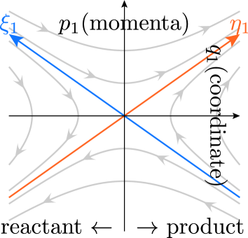
Figure 1: (color online). Phase space flow of the normal mode with negative curvature (hyperbolic degree of freedom). Reactant and product are defined by the sign of $q_{1}$. $\eta_{1}=0$(or $\xi_{1}$-axis) divides the destination of trajectories; Trajectories in $\eta_{1}>0$ go into the product side ($q_{1}>0$) as $t\rightarrow+\infty$ and those in $\eta_{1}<0$ go into the reactant side ($q_{1}<0$). Similarly, $\xi_{1}=0$(or $\eta_{1}$-axis) divides the origin of trajectories; Trajectories in $\xi_{1}>0$ originate from the reactant side and those in $\eta_{1}<0$ from the product side.

Here one can introduce the following coordinates

$$\eta_{j}= (p_{j}+\lambda_{j}q_{j})/(\lambda_{j}\sqrt{2}),~{}~{}~{}\xi_{j}= (p_{j}-\lambda_{j}q_{j})/\sqrt{2},$$ (2)

corresponding to eigenvectors of the coefficient matrix of the linear differential equation (Eq. 1) with eigenvalue $\lambda_{j}=\pm\sqrt{-k_{j}}$. Here one can also introduce another set of coordinates

$$I_{j}= \xi_{j}\eta_{j},~{}~{}~{}\theta_{j}= \ln|\lambda_{j}\eta_{j}/\xi_{j}|/2,$$ (3)

called “action” and “angle” variables. When Eq. (1) holds, the action variable is an integral of motion, and trajectories run along the hyperbolas given by $I_{j}=\mathrm{const.}$ shown by gray lines in Fig. 1. The $\eta_{j}$- and $\xi_{j}$-axes run along the asymptotic lines of the hyperbolas in Fig. 1. The Hamiltonian equation of motion can be written as

$$\dot{{\bm{\zeta}}}_{j}\approx-L_{H_{0}}{\bm{\zeta}}_{j}=-\lambda_{j}L_{I_{j}}{\bm{\zeta}}_{j},=\begin{pmatrix}-\lambda_{j}&0\cr 0&\lambda_{j}\end{pmatrix}{\bm{\zeta}}_{j},$$ (4)

where ${\bm{\zeta}}_{j}=(\xi_{j},\eta_{j})^{\mathrm{T}}$, and the Lie derivative $L_{F}$ is defined as $L_{F}{\bm{\zeta}}_{k}=\{F,{\bm{\zeta}}_{k}\}=\sum_{j=1}^{n}\frac{\partial F}{\partial\eta_{j}}\frac{\partial{\bm{\zeta}}_{k}}{\partial\xi_{j}}-\frac{\partial F}{\partial\xi_{j}}\frac{\partial{\bm{\zeta}}_{k}}{\partial\eta_{j}}$. One can tell the destination region and the origin region of trajectories from the signs of $\eta_{j}$ and $\xi_{j}$ as follows: If $\eta_{j}>0$, the trajectory goes into $q_{j}>0$ and if $\eta_{j}<0$, then the trajectory goes into $q_{j}<0$. Therefore one can tell the destination of trajectories from the sign of $\eta_{j}$. Similarly, the origin of trajectories can be told from the sign of $\xi_{j}$. Hereafter we call the set $\eta_{j}=0$ “destination-dividing set,” and $\xi_{j}=0$ “origin-dividing set,” and each of these two sets constitute “reactivity boundaries”.

When the NM picture dominates the dynamics around the stationary point, the form of Eq. (4) enables us to identify the fate of reaction. This is also generally the case if one can achieve a canonical transformation to turn the Hamiltonian into the form of $H=H({\bm{I}})$, even though $\lambda_{j}$s are depends on initial ${I_{j}}$s . This transformation has been mostly achieved by the normal form theory based on expansion around a single stationary point. The theory has been applied and developed to elucidate the mechanism of several reaction dynamics about a decade Komatsuzaki and Berry (1999, 2001); Wiggins et al. (2001); Uzer et al. (2002); Bartsch et al. (2005); Li et al. (2006); Kawai and Komatsuzaki (2010); Hernandez et al. (2010); Kawai and Komatsuzaki (2011a); Waalkens et al. (2008); Kawai and Komatsuzaki (2011b, c); Ünver Çiftçi and Waalkens (2012); Teramoto et al. (2011); Toda et al. (2005); Komatsuzaki et al. (2011). For practical applications the Lie canonical perturbation theory, developed by a Japanese astrophysicist Gen-Ichiro HoriHori (1966, 1967) (and equivalent theory was independently developed by DepritCampbell and Jefferys (1970); Deprit (1969)), has been frequently used.

II.2 Reactivity boundary

For complex molecular systems, the potential energy surface becomes more complicated, and a single transition from a potential basin to another involves not only index-one saddles but also higher index saddles. The normal form theory shown in Sec. II.1, based on expansion around a single stationary point, may not work well for such complex systems, where the fate of the reaction may not be dominated solely by the local property of the potential around the point. Therefore the definition of the reactivity boundaries should not be based on perturbation theory. In this subsection, we seek for a more general definition of reactivity boundaries, so that the definition can describe invariant objects previously studied (such as impenetrable barriersWiggins et al. (2001) and reactive islandde Almeida et al. (1990)), to analyze more complicated reactions by following the Pechukas’ foresightPechukas (1976).

A “state,” which may refer to reactant or product, forms a certain region in the phase space $\Omega$. Let us denote the states by $S_{1},\dots,S_{N}$, which are disjoint subsets of $\Omega$ ($S_{j}\subset\Omega$ and $S_{i}\cap S_{j}=\emptyset$ where $i,j=1,2,\dots,N$ and $i\neq j$). In between the regions corresponding to the states, there can be intermediate an region $\Omega_{0}$ that do not belong to any of the states (Fig. 2): $\Omega=S_{1}\sqcup\dots\sqcup S_{N}\sqcup\Omega_{0}$. Most of the trajectories in the intermediate region eventually go into either of the states as time proceeds. Likewise, when propagated backward in time, most of them turn out to originate from either of the states. Consider a set of trajectories that originate from the state $S_{1}$ and go into the state $S_{2}$ ($\mathrm{r}_{12}$ in Fig. 2), and another set consisting of trajectories that originate from $S_{1}$ and go back into the same state $S_{1}$ ($\mathrm{n}_{1}$ in Fig. 2). In between these two sets of trajectories there may lie a boundary which consists of trajectories that do not go into either of the states ($\mathrm{d}_{1}$ in Fig. 2). In the cases discussed in Sec. II.1, such trajectories were seen to asymptotically approach into some invariant set(s) in the intermediate region. Suppose there exist such an invariant set $\Omega_{S}$, which is a co-dimension two subset of $\Omega_{0}$. We then consider co-dimension one subset $\Omega_{OD},\Omega_{DD}\subset\Omega_{0}$ satisfying $\lim_{T\rightarrow\infty}\phi^{T}(\Omega_{OD})=\Omega_{S}$ and $\lim_{T\rightarrow-\infty}\phi^{T}(\Omega_{DD})=\Omega_{S}$ as follows:

• Destination-dividing set $\Omega_{DD}$ ($\mathrm{d}_{1}$ and $\mathrm{d}_{2}$ in Fig. 2)
  A set of trajectories whose origin belongs to a certain state but whose destination does not belong to any state.

• Origin-dividing set $\Omega_{OD}$ ($\mathrm{o}_{1}$ and $\mathrm{o}_{2}$ in Fig. 2)
  A set of trajectories whose destination belongs to a certain state but whose origin does not belong to any state.

The former set constitutes a boundary dividing the destination regions of trajectories, whereas the latter constitutes a boundary dividing the origin regions of trajectories. The set of the trajectories (invariant set) that satisfy one of the above conditions will be called reactivity boundary in the following. The asymptotic limit $\Omega_{S}$ of the reactivity boundary, which belongs to neither reactant nor product, will be called “seed” of reactivity boundaries. The definition of the reactivity boundary (the destination- or the origin-dividing set) can apply systems with multiple states, since the definition of the reactivity boundaries are only based on a single state. This definition of the reactivity boundaries and their seed is a generalization of the previous invariant objects (the stable and unstable manifolds of NHIM, and the NHIM, respectively) studied in literature Komatsuzaki and Berry (1999, 2001); Wiggins et al. (2001); Uzer et al. (2002); Bartsch et al. (2005); Li et al. (2006); Kawai and Komatsuzaki (2010); Hernandez et al. (2010); Kawai and Komatsuzaki (2011a); Waalkens et al. (2008); Kawai and Komatsuzaki (2011b, c); Ünver Çiftçi and Waalkens (2012); Teramoto et al. (2011); Toda et al. (2005); Komatsuzaki et al. (2011) and summarized in Sec. II.1.

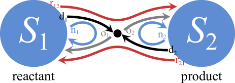
Figure 2: (color online). Blue large circles represent states $S_{1}$ and $S_{2}$. Arrows represent particular sorts of trajectories; blue arrows ($\mathrm{n}_{1}$ and $\mathrm{n}_{2}$) represent non-reactive trajectories, while red ones ($\mathrm{r}_{12}$ and $\mathrm{r}_{21}$) represent reactive trajectories. Black arrows ($\mathrm{d}_{1}$ and $\mathrm{d}_{2}$) and gray arrows ($\mathrm{o}_{1}$ and $\mathrm{o}_{2}$) represent trajectories in the destination-dividing set, and those in the origin-dividing set, respectively.

III Numerical Demonstrations

III.1 Three DoFs model of $\text{H}_{5}^{+}$

We demonstrate here a numerical calculation of the reactivity boundary defined in Sec. II with a model $\mathrm{H}_{5}^{+}$ system. This cation plays an important role in interstellar chemistry, especially because of the proton exchange reaction $\mathrm{H}_{3}^{+}+\mathrm{HD}\rightleftharpoons\mathrm{H}_{2}+\mathrm{H}_{2}\mathrm{D}^{+}$ occurring through the $\mathrm{H}_{4}\mathrm{D}^{+}$ intermediate. As shown in the previous ab initio calculation Xie et al. (2005), the most stable structure of the $\mathrm{H}_{5}^{+}$ system is a weakly bound cluster of $\mathrm{H}_{2}$ and $\mathrm{H}_{3}^{+}$ moieties, with the $\mathrm{H}_{2}$ standing perpendicular to the $\mathrm{H}_{3}^{+}$ molecular plane. Being a multi-body system, the $\mathrm{H}_{5}^{+}$ cation undergoes various isomerization reactions. Taking the four lowest stationary points (one minimum, two index-one saddle points, and one index-two saddle), we have two reaction directions. One is a torsional isomerization where the $\mathrm{H}_{2}$ flips by 180^∘ with the planar structure corresponding to the saddle point. The other is the proton exchange between the two moieties $\mathrm{H}_{2}+\mathrm{H}_{3}^{+}\rightleftharpoons\mathrm{H}_{3}^{+}+\mathrm{H}_{2}$.

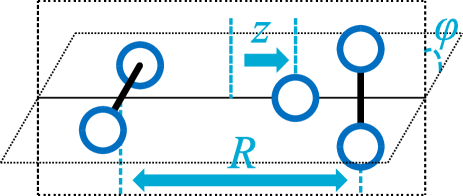
Figure 3: (color online). $\text{H}_{3}^{+}+\text{H}_{2}\rightarrow\text{H}_{2}+\text{H}_{3}^{+}$ reaction can be written by three coordinate $\varphi,R,z$ depicted on picture.

In the present investigation, we treat the dynamics of $\mathrm{H}_{5}^{+}$ by confining it into a three degrees-of-freedom system. The dynamical variables are the center-of-mass distance $R$ between the two $\mathrm{H}_{2}$ moieties, the position $z$ of the central hydrogen atom along the center-of-mass axis, and the torsional angle $\varphi$ of the two $\mathrm{H}_{2}$ as shown in Fig. 3. The coordinate $z$ corresponds to the proton exchange reaction between the two moieties, while the angle $\varphi$ corresponds to the torsional isomerization. We calculated the potential energy surface at the CCSD(T) level which is the same level with the previous calculation Xie et al. (2005). The ab initio calculations were performed at 439 points in the range $0\leq|z|\leq 0.4~{}\text{\AA}$ and $2.09~{}\text{\AA}\leq R\leq 2.51~{}\text{\AA}$, with the $\mathrm{H}_{2}$ bond lengths optimized for each given value of $(z,R,\varphi)$. By checking the energy value, this region was confirmed to be sufficient to describe the motion with total energy below 200 cm^-1. The potential energy values were then fitted to a cubic order polynomial in $(z^{2},R,\cos 2\varphi)$. The maximum fitting error was 0.8 cm^-1, sufficiently small considering the total energy 170 cm^-1 of the trajectories run in the present investigation. The structures and energies of the four lowest stationary points of the fitted surface are listed in Table 1 and compared with the literature values.Xie et al. (2005) The mathematical expression of the fitted potential energy surface is available as the supporting information to this article.

Table 1: Structures and energies of four lowest stationary points of $\mathrm{H}_{5}^{+}$. The energies are given relative to the first equilibrium point.

	$\varphi$	$R$ / Å	$z$ / Å	Energy / cm-1	Ref. Xie et al.,2005
1	$\pi/2$	2.18	0.19	(ref.)	(ref.)	global minimum
2	$\pi/2$	2.11	0	48.6	48.4	index-one saddle
3	0	2.19	0.21	95.9	96.4	index-one saddle
4	0	2.12	0	162.7	162.8	index-two saddle

We use this three-dimensional system as an illustrative model to demonstrate the concepts introduced in Sec. II. Note however that the real $\mathrm{H}_{5}^{+}$ system has larger DoFs (nine internal modes and three rotational modes). Quantum effects must also be considered for the complete treatment of this system. We here briefly mention that the concept of reactivity boundaries around the index-one saddle point has recently been extended to incorporate ro-vibrational couplingsKawai and Komatsuzaki (2011c); Ünver Çiftçi and Waalkens (2012) and quantum effectsWaalkens et al. (2008); Kawai and Komatsuzaki (2011b). It will be an important future work to combine these studies with the generalized reactivity boundaries proposed in the present paper. In the present numerical calculation we confine the system configuration into the three-dimensional subspace mentioned above for the sake of simplicity. We still note the global minimum, the three lowest saddle points and their unstable directions are all included in this subspace, while the motions transverse to this subspace are bath mode oscillations. This three-dimensional model is therefore expected to capture some of the essential properties of the isomerization and the proton exchange processes in the real $\mathrm{H}_{5}^{+}$ system with low energies.

There are two index-one saddle points, denoted as 2 and 3, that correspond to the proton exchange and the torsional isomerization, respectively. The highest of these four stationary points is an index-two saddle point, denoted as 4, representing a concerted reaction of the proton exchange and the torsion. Figure 4 depicts the two-dimensional potential energy surface in $z$ and $\varphi$ where the $R$ is relaxed to the minimum energy for each given value of $(z,\varphi)$. There are four symmetrically equivalent points corresponding to the global minimum 1. Similarly the saddle points 2, 3, and 4 have two, four, and two equivalent points, respectively.

The dynamical calculations of the present three-dimensional model of $\mathrm{H}_{5}^{+}$ are performed by integrating the equation of motion given by the following Hamiltonian

$$H=\frac{1}{I_{\varphi}}{p_{\varphi}}^{2}+\frac{1}{2\mu_{R}}{p_{R}}^{2}+\frac{1}{2\mu_{z}}{p_{z}}^{2}+V(\varphi,R,z),$$ (5)

where $p_{\varphi}$ is the angular momentum conjugate to the torsional angle $\varphi$, and $p_{R}$ and $p_{z}$ are the linear momenta conjugate to $R$ and $z$, respectively. The reduced masses are

$$\mu_{z}=\frac{4}{5}m_{\mathrm{H}}, \mu_{R}=m_{\mathrm{H}},$$ (6)

where $m_{\mathrm{H}}$ is the mass of the hydrogen atom, and $I_{\varphi}$ is the moment of inertia of H₂.

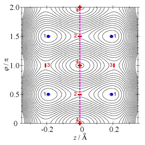
Figure 4: The potential energy surface as a function of $z$ and $\varphi$, representing the proton exchange and the torsional motion, where the other coordinate $R$ is optimized at each point $(z,\varphi)$. Each number corresponds to each stationary point listed in Table 1. Blue points, red bars, and red cross denote the potential minima, index-one saddles, and index-two saddle, respectively. Contours are spaced with 10 cm^-1. The initial condition for the calculation of the reactivity boundaries are prepared at $z=0$, where index-one saddle points 2 and index-two saddle points 4 are located (pink dashed line).

III.2 Reactivity boundary in $\text{H}_{5}^{+}$

As described in Sec. II.2, the reactivity boundary typically consists of trajectories emanating from an invariant manifold in the intermediate region. It is calculated by propagating the system, either forward or backward in time, from the close vicinity of the invariant manifold. In the present investigation we focus on the proton exchange reaction from $\mathrm{H}_{2}+\mathrm{H}_{3}^{+}$ to $\mathrm{H}_{3}^{+}+\mathrm{H}_{2}$, to demonstrate the extraction of reactivity boundary. The configuration $\mathrm{H}_{2}+\mathrm{H}_{3}^{+}$ corresponds to a region with $z>0$ and $\mathrm{H}_{3}^{+}+\mathrm{H}_{2}$ with $z<0$. The intermediate region thus lies on some region around $z=0$. In this case the surface defined by $z=0$ and $p_{z}=0$ serves as an invariant manifold due to the symmetry of the system. This means that, once the system stays on that surface, it does perpetually irrespective of what values the other variables take. This invariant manifold is unstable in that any infinitesimally small deviation from the surface of $z=0$ and $p_{z}=0$ makes the system depart from the surface and fall down into one of the four well regions shown in Fig. 4. Therefore the reactivity boundaries are stable and unstable manifolds of $z=0,p_{z}=0$ in this case. The extraction of reactivity boundary can be carried out as follows: we first uniformly sample phase space points $(p_{z}=0,p_{R},p_{\varphi},z=0,R,\varphi)$ at a given total energy in that invariant manifold (see also Appendix for details). Second, we give the system a small positive deviations in $p_{z}$, and propagate it forward in time (corresponding to the origin-dividing set o₂ in Fig. 2). Those trajectories correspond to the generalization of $\xi_{1}=0$ with positive $\eta_{1}$ to divide the origin of trajectories for normal mode approximation in Fig. 1. Likewise, the propagation of the system backward in time results in trajectories that divide the destination of trajectories, corresponding to the set d₂ in Fig. 2 (Compare also with $\eta_{1}=0$ with negative $\xi_{1}$ for normal mode Hamiltonian in Fig. 1). Note here again that the generalization involves two essential differences from the normal mode picture: one is the generalization to nonlinear Hamiltonian systems in which normal mode approximation does not hold, and the other is that the invariant manifold from which reactivity boundaries emanate can be associated not only with a single saddle point but with multiple saddle points with different indices.

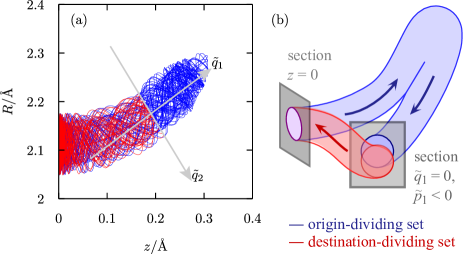
Figure 5: (color online). The reactivity boundaries of $\text{H}_{3}^{+}+\text{H}_{2}\rightarrow\text{H}_{2}+\text{H}_{3}^{+}$ reaction. (a) randomly sampled fifty trajectories from the destination-dividing set (red) and the origin-dividing set (blue), both constituting the reactivity boundaries, initiated from the section of $z=0$ and $p_{z}\simeq 0$ projected on the $z-R$ space. The normal mode coordinates $\tilde{q}_{1}$ and $\tilde{q}_{2}$ at the potential minimum are shown by gray lines. (b) a schematic picture of reactivity boundaries depicted as “tubesde Almeida et al. (1990)” departing from $z=0$ and $p_{z}\simeq 0$. Note here that the invariant manifold of $z=0$ and $p_{z}=0$ can involve multiple saddle points.

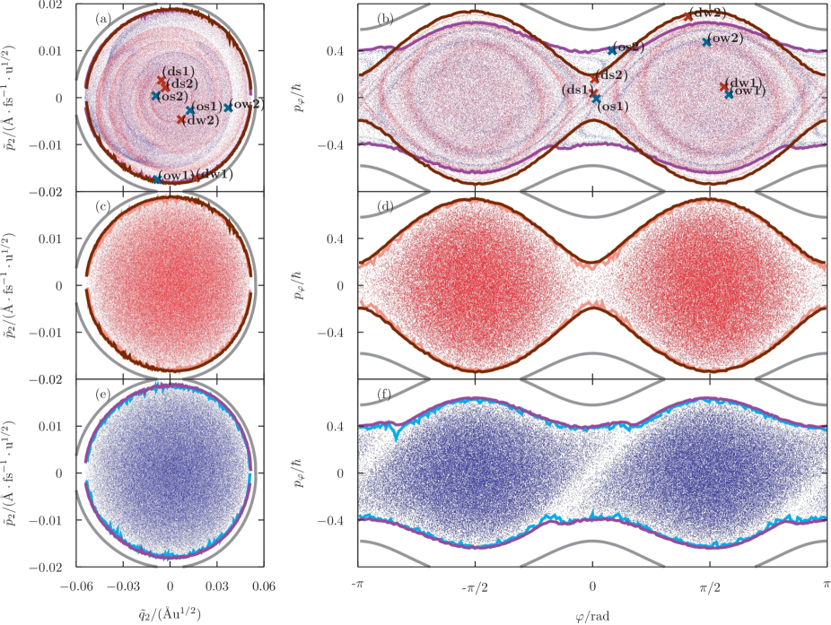
Figure 6: (color online). The reactivity of $\text{H}_{3}^{+}+\text{H}_{2}\rightarrow\text{H}_{2}+\text{H}_{3}^{+}$ reaction on the section of $\tilde{q}_{1}=0,\tilde{p}_{1}<0$. 100,000 trajectories are uniformly sampled on the surface of $z=0$ with positive momentum $p_{z}\simeq 0$ and evolved forward in time until they cross a surface defined by $\tilde{q}_{1}=0$ and $\tilde{p}_{1}<0$ by the normal mode coordinate $\tilde{{\bm{q}}}$ and its conjugate momentum $\tilde{{\bm{p}}}$ at the potential minimum (see also Appendix for details). The trajectories forming the origin-dividing set are shown by blue dots. Likewise, 100,000 trajectories are similarly sampled on that surface with negative $p_{z}\simeq 0$ and propagated backward in time until they cross the surface. The trajectories forming the destination-dividing set are shown by red dots. (a) and (b): the projections of the first intersections of the destination-dividing set (red dots) and the origin-dividing set (blue dots) crossing the surface of $\tilde{q}_{1}=0$ and $\tilde{p}_{1}<0$ on the section, respectively, onto the $\tilde{q}_{2}$-$\tilde{p}_{2}$ space and the $\varphi$-$p_{\varphi}$ space. The gray lines denote the boundaries of energetically inaccessible region. The values are defined by maximum and minimum of $p_{\varphi}$ at each $\varphi$. The cross symbols (dw1, dw2,…) represent the initial positions (on that place) of the trajectories shown in 7. (c), (d), (e), (f): the projections of the phase space points that are going into the product side (red dots) and those that have come from the product side (blue dots) are depicted to conform “inside” of reactivity boundaries and to check validity of the extraction of the reactivity boundaries. Orange lines in (c) and cyan lines (e) are maximum/minimum $\tilde{p}_{2}$ of the sets of the reactive points. Brown lines in (c) and purple lines (e) are maximum/minimum $\tilde{p}_{2}$ of the reactivity boundaries. Similarly, Orange lines in (d) and cyan lines (f) are maximum/minimum $p_{\varphi}$ of the sets of the reactive points. Brown lines in (d) and purple lines (f) are maximum/minimum $p_{\varphi}$ of the reactivity boundaries.

Figure 5 shows randomly chosen fifty samples from the origin-dividing set (blue) and the destination-dividing set (red) depicted on the $R$-$z$ space. The reactivity boundaries are only drawn until they first cross the section defined by $\tilde{q}_{1}=0$ and $\tilde{p}_{1}<0$ by the normal mode coordinate $\tilde{{\bm{q}}}$ and its conjugate momentum $\tilde{{\bm{p}}}$ at the potential minimum (the normal mode coordinates are shown by the gray arrows in Fig. 5 (a)). The reactivity boundaries are four dimensional surfaces in an equienergy shell which divide reactive and non-reactive trajectories as schematically shown in Fig. 5(b). Figures 6(a)(b) show the origin dividing set (blue) and the destination dividing set (red) on the $\tilde{q}_{1}=0,\tilde{p}_{1}<0$ section depicted by using 100,000 trajectories whose initial conditions are uniformly sampled on the $z=0,p_{z}\simeq 0$ section (see also Appendix for details). Let us look into how reaction selectivity existing in the phase space can be rationalized or visualized in these projections. In Fig. 6(a), one can find few fingerprints of the reaction selectivity existing in the phase space with respect to the signs of the normal mode coordinate and momentum. The reaction path is curved in the $R$-$z$ space as shown in Fig. 5(a) and the saddle points exist on the negative side of $\tilde{q}_{1}$. Because Fig. 6(a) is the projection of the first intersections of the reaction boundaries across the surface of $\tilde{q}_{1}=0$ and $\tilde{p}_{1}<0$ (i.e., all dots on Fig. 6(a) are moving towards the surface of $z=0$), one may expect that $\tilde{q}_{2}<0$ or $\tilde{p}_{2}<0$ on that surface should enhance the reaction probability, resulting in a nonuniform distribution of the reaction boundaries on the $\tilde{p}_{2}$-$\tilde{q}_{2}$ space. However, as seen in Fig. 6(a), the reaction boundaries are distributed rather uniformly in this space (e.g., no preference in the sign of $\tilde{p}_{2}$). This implies that preparing $\tilde{q}_{2}<0$ or $\tilde{p}_{2}<0$ on that surface does not increase the ability of the system to climb the reaction barrier. As shown in Fig. 5 (a), the trajectories oscillate rapidly in the $\tilde{q}_{2}$-direction and the bath mode coordinate change its sign many time before coming close to $z=0$, where the saddle points 2 and 4 for the proton transfer reaction are located, while they slowly adapt to the curved reaction pathway. The dynamics near the index-one and index-two saddle points, thus, seems not to be sensitive to the initial vibrational phase prepared in the well region.

Next let us turn to the $p_{\varphi}$-$\varphi$ projection in Fig. 6(b). The reaction boundaries, both the destination dividing set (red points in the figure) and the origin dividing set (blue), are confined in smaller values of $|p_{\varphi}|$ compared to energetically accessible values. This is because the energy is more distributed into the reactive mode when the momentum in the $\varphi$-direction is smaller. In contrast to the $\tilde{p}_{2}$-$\tilde{q}_{2}$ space, the reaction selectivity existing in the phase space manifests nonuniformity of the distribution of these reaction boundaries in the $p_{\varphi}$-$\varphi$ space. The confinement of the destination-dividing set (red) in smaller $|p_{\varphi}|$ is more pronounced in $\varphi\approx 0$ than in $\varphi\approx\pi/2$, while the range of $|p_{\varphi}|$ of the origin-dividing set (blue) is more uniform in $\varphi$. Note that $\varphi=0$ corresponds to the planar configurations that involve both the index-one saddle points 3 and the index two saddle points 4 (see Table 1) and the reaction must proceed over the index-two saddle when $\varphi\approx 0$ (Fig. 4). The relative barrier height through the index-two saddle 4 for the proton transfer with $\varphi=0$ is $162.7-95.9=66.8\ \mathrm{cm}^{-1}$ which is higher than the barrier height through the index-one saddle 2 with $\varphi=\pi/2$, 48.6 cm^-1 as seen from Table 1. In order to put sufficient energy into the reactive mode to overcome the barrier, therefore, the momentum $p_{\varphi}$ in the $\varphi$-direction must be confined into much smaller values $|p_{\varphi}|$ for $\varphi\approx 0$ than for $\varphi\approx\pi/2$ due to the conservation of total energy of the system. This interpretation, done by the relative barrier height with constant $\varphi$, is consistent with the plot of the sample trajectory (ds1) for small initial $|p_{\varphi}|$ in Fig. 7. shows some representative sample trajectories in the $\varphi$-$z$ and $R$-$z$ spaces, whose locations in the $\tilde{p}_{2}$-$\tilde{q}_{2}$ and the $p_{\varphi}$-$\varphi$ spaces are also indicated as symbols in Figs. 6(a)(b). It is seen that the motions along the reactive direction (approximately the $z$-direction) take place more rapidly than that along the $\varphi$-direction and the value of $\varphi$ does not change much during the course of the reaction.

On the other hand, the trajectories approaching to the surface of $z=0$ and $p_{z}<0$ with large values of $|p_{\varphi}|$ at $\varphi\approx\pi/2$ at the section correspond to the motion starting from the well region and approach to the index-two saddle 4, as shown in the $z-\varphi$ plane in Fig. 7 (dw2). This is contrasted with the trajectories starting with small $|p_{\varphi}|$ at $\varphi\approx\pi/2$ and approaching to the index-one saddle 2 (dw1). If we regard $(p_{\varphi},\varphi)$ as roughly corresponding to the nonreactive mode, this situation seems to be counter-intuitive in that when the nonreactive degree of freedom is more excited (i.e., larger $|p_{\varphi}|$) the system is more likely to approach to the higher index-saddle with larger barrier height. This arises from the fact that the “reaction direction” for proton transfer through the index-two saddle is not simply along $z$ but runs diagonal in the $z$-$\varphi$ plane as the system goes from the well directly to the index-two saddle 4. The large momentum $|p_{\varphi}|$ is also used for approaching to the higher barrier of the index-two saddle 4 and, therefore, the large initial value $|p_{\varphi}|$ is favored for the reaction over the index-two saddle. All the above discussions explain the nonuniformity of the range of $p_{\varphi}$ with respect to $\varphi$ for the destination-dividing set (red) in Fig. 6 (b).

Compared to the destination-dividing set, the origin-dividing set is more uniformly distributed along $\varphi$ (see blue dots in Fig. 6 (b)). This arises from the choice of the cross section for observing the reaction boundaries. We chose the section of $\tilde{q}_{1}=0$ with $\tilde{p}_{1}<0$ that is located at the potential minimum. With this choice, we are observing the origin-dividing set after it is bounced by the potential wall in the large-$z$ region (Fig. 5 (a)). As seen in the sample trajectories (os1),(os2),(ow1),(ow2) in Fig. 7, the value of $\varphi$ changes during the stay in the well region. The change of $p_{\varphi}$ due to the energy exchange between the $\varphi$-mode and the others can also be seen by the direction of the trajectories. Therefore the longer time between the preparation (at $z=0$) and the observation ($\tilde{q}_{1}=0$ with $\tilde{p}_{1}<0$) of the destination-dividing set than the origin-dividing set causes some further “mixing” in ($\varphi,p_{\varphi})$ and the reaction selectivity is lost compared to the direct cross section as observed for the destination-dividing set in Fig. 6.

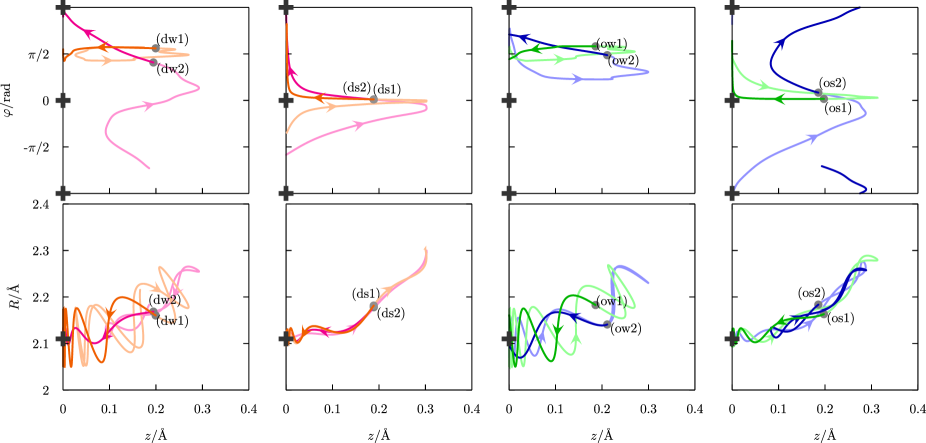
Figure 7: (color online). The representative sample trajectories forming the reactivity boundaries in Fig. 6(a) and (b) on the $\varphi$-$z$ space and the $R$-$z$ space. The gray points denote the locations in these spaces when those sample trajectories intersect the section of $\tilde{q}_{1}=0$ with $\tilde{p}_{1}<0$. The symbol $+$ denotes the location of the index-one point 2 or index-two saddle point 4. The difference of the location of the two saddle points is invisible in the $R$-$z$ projection with this resolution. The magenta and orange colored trajectories are of the destination dividing set. The blue and green colored trajectories are of the origin dividing set. The color grade represents the time course of trajectories obeying the Hamiltonian: time goes from the light to the dark grade, and the light and dark correspond to before and after the intersection of the section of $\tilde{q}_{1}=0$ with $\tilde{p}_{1}<0$. For instance, trajectory (dw2) indicates that of the destination-dividing set in the well region with ‘large’ $|p_{\varphi}|$. Trajectory (os1) indicates that of the origin-dividing set at the index-one saddle region with ‘small’ $|p_{\varphi}|$.

Reactivity boundaries are four dimensional objects, and we cannot capture their full characteristics by the two dimensional projections. In contrast to normal mode approximation or normal form theory locally expanded in the vicinity of a single saddle point, for our present general footing, the analytic formula of the underlying reaction coordinate is hard to derive and the invariant manifold locally extracted in the vicinity of a single point or a collection of multiple saddle points with different indices might not necessarily provide the boundary to divide the fates of the reactions originated from the well region far apart from the saddles.Nagahata et al. (2013)

To check the validity of our numerical extraction of reactivity boundaries, we note the fact that both reactive and non-reactive trajectories must exist in the vicinity of the reactivity boundaries. We therefore check the reactivity of trajectories in the vicinity of each sampled point $(\tilde{p}_{2},\tilde{q}_{2},\varphi,p_{\varphi})$ on the reactivity boundaries on the section. Sampling was made of phase space points $(\tilde{p}_{2}^{\prime},\tilde{q}_{2}^{\prime},\varphi^{\prime},p_{\varphi}^{\prime})$ that satisfy

$$\left|\frac{\tilde{p}_{2}^{\prime}-\tilde{p}_{2}}{0.02\text{\AA}\mathrm{u^{1/2}fs^{-1}}}\right|^{2}+\left|\frac{\tilde{q}_{2}^{\prime}-\tilde{q}_{2}}{0.06\text{\AA}\mathrm{u^{1/2}}}\right|^{2}$$ (7)

$$+\left|\frac{\varphi^{\prime}-\varphi}{\pi}\right|^{2}+\left|\frac{p_{\varphi}^{\prime}-p_{\varphi}}{0.8\hbar}\right|^{2} =10^{-20}$$ (8)

for all the sampled points $(\tilde{p}_{2},\tilde{q}_{2},\varphi,p_{\varphi})$ of the reactivity boundaries. As expected, both reactive and non-reactive trajectories were found from this sampling (data not shown).

To give more visual representation for the validity of our numerical extraction of reactivity boundaries, we uniformly sampled 1,000,000 points on the $\tilde{q}_{1}=0,\tilde{p}_{1}<0$ section in the well region and propagated them forward and backward in time. The phase space points that turned out to go into the other well region in the forward time propagation are shown in (c) and (d) in Fig. 6 by projection on the $\tilde{q}_{2}-\tilde{p}_{2}$ space and the $\varphi-p_{\varphi}$ space. Those that turned out to have come from the other well in the backward propagation are shown in (e) and (f). Of the total 1,000,000 sampled points, about 100,000 were found to be reactive trajectories. As can be seen in Fig. 6(c)-(f), a good coincidence was observed in the maximum/minimum $\tilde{p}_{2}$ and $p_{\varphi}$ at each $\tilde{q}_{2}$ and $\varphi$ between the reactive trajectories (corresponding to the inside of “tubesde Almeida et al. (1990)” in Fig. 5(b)) and the reactivity boundaries. In any neighborhood of the reactivity boundaries extracted from the surface of $z=0$ and $p_{z}\simeq 0$ apart from the well regions, reactive trajectories exist in the projected space. The results, therefore, also give some support (necessary condition) to the validity of the reactivity boundaries calculated in the present investigation.

IV Conclusion and Perspectives

In this article, the concept of reactivity boundary, which is an invariant manifold lying between reacting and non-reacting trajectories in the phase space, was revisited and generalized. It is defined as a set of trajectories that converge into a seed of reactivity boundaries. The latter is located between the reactant and the product regions, and goes neither into the reactant or the product, in either forward or backward time propagation. When only one saddle point controls the reaction dynamics and the energy is not very high above the saddle point, the reactivity boundaries are readily extracted analytically by normal form theory. The definition given here is, however, not limited to such cases but generalized to a single reaction passing through multiple saddle points including higher index saddles.

The reactivity boundaries constitute a skeleton of the phase space of the reaction system. Observation of their locations in certain cross sections tells which initial conditions can lead to chemical reactions. We applied the concept of the reactivity boundaries to the three-dimensional model system of the proton exchange reaction associated with a bottleneck made up of two index-one saddles (2) and two index-two saddles (4) in $\mathrm{H}_{5}^{+}$ cation. The bath mode vibration represented by the normal mode $(\tilde{p}_{2},\tilde{q}_{2})$ was found to be almost separate from the reactive mode, and the fast change of its vibrational phase masked the reaction selectivity existing in the phase space.

On the other hand, the reaction selectivity in the phase space manifested high degree of selectivity for the torsional motion, related to the existence of multiple types of saddle points for different values of the torsion angle. In addition to the reaction through the index-one saddle 2 of the proton exchange, two limiting behaviors of reacting trajectories were identified. In one group, the trajectories go from the index-one saddle 3 of the torsion isomerization to the index-two saddle 4. Small initial values of the torsional angular momentum $|p_{\varphi}|$ is favored for this reaction pathway because of the high energy difference between the index-two saddle point 4 and the index-one torsion saddle point 3. The other group of the reacting trajectories is those going directly from the well region to the index-two saddle 4. For this group, high initial values of $|p_{\varphi}|$ is favored because the reaction pathway runs diagonal in the $z$-$\varphi$ plane rather than parallel to the $z$-direction. These pictures of the reaction dynamics were obtained with the help of the concept of reactivity boundaries stated in the present paper.

In this article we have focused on the first intersection of the reactivity boundaries across the section of $\tilde{q}_{1}=0$ with $\tilde{p}_{1}<0$ located in the well region. This corresponds to the fast stage of the reaction process, that is, “before leaving from that well” and “after entering with one reflection back by the potential wall in that well.” Reactivity boundaries also enable us to quantify the slow stage of the process by the projection of the second, third, fourth intersections of the boundaries onto, e.g., the $\varphi-p_{\varphi}$ space. Distributions of such intersections on some projected spaces can trace how statistical properties may emerge for slower timescales (yielding a more uniform distribution), making conventional statistical rate theories applicable. Note that as demonstrated in this article the first intersection corresponding to the reactive initial conditions are distributed in a nonuniform manner, to which conventional statistical rate theories are not applicable. The essential understanding of reactions requires reactivity boundaries that enable us to predict the fate of reactions independent of which timescale to be considered.

In the extraction scheme of reaction boundary presented in Sec. II.2, we have not restricted the definition of states to a local equilibrium state in which highly-developed chaos is implicitly postulated. As known, at least for two DoFs systems in Ref. Davis and Gray, 1986; Mackay et al., 1984, there may exist several dynamic states within a single potential well whose number and the reaction rate constants among them are energy-dependent. The definition of states in Sec. II.2 can involve such nonergodic states. In addition, as discussed in the text, the seed of reactivity boundaries existing in between the states involves not necessarily only one single saddle point but also several saddle points with different indices.

The practical methods for extracting the reactivity boundaries, however, need still much to be considered. When only one saddle point plays a dominant role in determining the occurrence of the reaction, normal form theory readily extracts the seed of reactivity boundaries in the analytical way. In contrast, there is still no practical method applicable to general cases where more than one saddle points are involved in the reaction process. In the present investigation, because of the preknowledge concerning the existence of symmetry, we can identify the seed of reactivity boundaries in the intermediate region. When the symmetry cannot be exploited easily, it is still a challenging future work to devise convenient methods to extract seeds of reactivity boundariesNagahata et al. (2013).

V Acknowledgment

TK has greatly benefited and been inspired from many discussions with Prof. Oka and his enthusiasm on how new concepts emerge more than we may expect when two different disciplines meet with each other such as chemistry and astronomy in nature. TK would like to dedicate this article using the concept of chemistry and celestial mechanics to him in token of his gratitude for Prof. Oka’s insightful thought. This work has been partially supported by JSPS, Research Center for Computational Science, Okazaki, Japan, Grant-in-Aid for Young Scientists (B) (to SK), Grant-in-Aid for challenging Exploratory Research (to TK), and Grant-in-Aid for Scientific Research (B) (to TK) from the Ministry of Education, Culture, Sports, Science and Technology.

VI Appendix: Uniform sampling

Here we explain how we sample the uniform distributions under constraints to depict the reactivity boundaries and the sets of reacted/reacting trajectories, i.e., those having just crossed the surface of $z=0$ from the product well and those being about to cross the surface, in the reactant well described in Sec. IIIB. To depict reactivity boundaries, we sample the position coordinate $(R,\varphi)$ according to the following distributions.

$$\rho(R,\varphi;z=0,p_{z}=0,H=E)$$

$$\propto\int\delta(E-H(\mathbf{p},\mathbf{q}))\delta(z)\delta(p_{z})dp_{R}dp_{z}dp_{\varphi}dz$$

$$\propto\sqrt{E-V(R,\varphi;z=0)}.$$ (9)

Here we define $\bar{\rho}_{\text{sd}}(R,\varphi)=\sqrt{\frac{E-V(R,\varphi;z=0)}{E-V_{0}}}$ yielding $0<\bar{\rho}_{\text{sd}}<1$, where $V_{0}=\min_{R,\varphi}V(R,\varphi;z=0)$. We employ the rejection method Press et al. (2007) to sample phase space points with the distribution $\bar{\rho}_{\text{sd}}$. We first sample points uniformly in the range of $\varphi\in[-\pi,\pi]$ and $R\in[2\text{\AA},2.2\text{\AA}]$ which include the whole energetically accessible region. The point is accepted or rejected by the following criterion:

$$\begin{cases}\text{accept}&\bar{\rho}_{\text{sd}}(R,\varphi)>\text{RAND},\\ \text{reject}&\text{otherwise},\end{cases}$$ (10)

where $\mathrm{RAND}$ is a uniform random number from $0$ to $1$. Then we perform sampling of the momentum for each sampled configuration as follows:

$$p_{R}=\sqrt{2(E-V)}\sin\theta/m_{R},$$

$$p_{\varphi}=\sqrt{2(E-V)}\cos\theta/(I_{\varphi}/2),$$

where $\theta$ is a uniform random number from $-\pi$ to $\pi$.

Similarly, to depict the sets of reacted/reacting trajectories in the reactant well, we sample phase space points according to the following distribution:

$$\rho(\tilde{q}_{2},\varphi;\tilde{q}_{1}=0,\tilde{p}_{1}<0,H=E)$$

$$\propto\int\delta(E-H(\mathbf{p},\mathbf{q}))\Theta(-\tilde{p}_{1})\delta(\tilde{q}_{1})d\tilde{p}_{1}d\tilde{p}_{2}d\tilde{p}_{\varphi}d\tilde{q}_{1}$$

$$\propto E-V(\tilde{q}_{2},\varphi;\tilde{q}_{1}=0).$$ (11)

Here $\Theta(x)$ is the Heaviside step function, and we define $\bar{\rho}_{\text{wl}}(\tilde{q}_{2},\varphi)=(E-V(\tilde{q}_{2},\varphi;\tilde{q}_{1}=0))/(E-V_{0})$, yielding $0<\bar{\rho}_{\text{wl}}<1$, where $V_{0}=\min_{\tilde{q}_{2},\varphi}V(\tilde{q}_{2},\varphi;\tilde{q}_{1}=0)$. We sample points uniformly in the range of $\varphi\in[-\pi,\pi]$ and $\tilde{q}_{2}\in[-0.15\text{\AA}\mathrm{u^{1}/2},0.15\text{\AA}\mathrm{u^{1}/2}]$ which include the whole energetically accessible region on this section. We apply the same rejection method Press et al. (2007) to construct $\bar{\rho}_{\text{wl}}$ distribution

$$\begin{cases}\text{accept}&\bar{\rho}_{\text{wl}}(\tilde{q}_{2},\varphi)>\text{RAND},\\ \text{reject}&\text{otherwise}.\end{cases}$$ (12)

Then we perform sampling of the momentum for each sampled configuration as follows:

$$\begin{cases}\text{accept}&\sin\theta_{1}>\text{RAND},\\ \text{reject}&\text{otherwise}.\end{cases}$$ (13)

$$\tilde{p}_{\varphi} = \sqrt{2(E-V)}\sin\theta_{1}\sin\theta_{2},$$

$$\tilde{p}_{1} = -\sqrt{2(E-V)}\cos\theta_{1},$$

$$\tilde{p}_{2} = \sqrt{2(E-V)}\sin\theta_{1}\cos\theta_{2},$$

since coordinate transformation to polar coordinates introduces phase space Jacobian $J=2(E-V)\sin\theta_{1}$, where $\theta_{1},\theta_{2}$ are uniform random numbers from $0$ to $\pi/2$ and from $-\pi$ to $\pi$, respectively.

References

- Pechukas (1976) P. Pechukas, in Dynamics of Molecular Collisions Part B, Modern Theoretical Chemistry, edited by W. H. Miller (Plenum Publishing Corporation, New York, 1976) Chap. 6, pp. 269–322.
- Pechukas and Pollak (1977) P. Pechukas and E. Pollak, J. Chem. Phys. 67, 5976 (1977).
- Sverdlik and Koeppl (1978) D. Sverdlik and G. Koeppl, Chem. Phys. Lett. 59, 449 (1978).
- Pollak and Pechukas (1978) E. Pollak and P. Pechukas, J. Chem. Phys. 69, 1218 (1978).
- Pechukas and Pollak (1979) P. Pechukas and E. Pollak, J. Chem. Phys. 71, 2062 (1979).
- Pollak and Pechukas (1979) E. Pollak and P. Pechukas, J. Chem. Phys. 70, 325 (1979).
- Child and Pollak (1980) M. S. Child and E. Pollak, J. Chem. Phys. 73, 4365 (1980).
- Pollak et al. (1980) E. Pollak, M. S. Child, and P. Pechukas, J. Chem. Phys. 72, 1669 (1980).
- Pollak and Levine (1980) E. Pollak and R. D. Levine, J. Chem. Phys. 72, 2990 (1980).
- Pollak and Child (1980) E. Pollak and M. S. Child, J. Chem. Phys. 73, 4373 (1980).
- Pechukas (1981) P. Pechukas, Annu. Rev. Phys. Chem. 32, 159 (1981).
- Pollak (1981a) E. Pollak, J. Chem. Phys. 74, 5586 (1981a).
- Pollak (1981b) E. Pollak, Chem. Phys. 61, 305 (1981b).
- Pollak (1981c) E. Pollak, Chem. Phys. Lett. 80, 45 (1981c).
- Wall et al. (1958) F. T. Wall, L. A. Hiller, and J. Mazur, J. Chem. Phys. 29, 255 (1958).
- Wall et al. (1961) F. T. Wall, L. A. Hiller, and J. Mazur, J. Chem. Phys. 35, 1284 (1961).
- Wall and Porter (1963) F. T. Wall and R. N. Porter, J. Chem. Phys. 39, 3112 (1963).
- Wright et al. (1975) J. S. Wright, G. Tan, K. J. Laidler, and J. E. Hulse, Chem. Phys. Lett. 30, 200 (1975).
- Wright (1976) J. S. Wright, J. Chem. Phys. 64, 970 (1976).
- Wright and Tan (1977) J. S. Wright and K. G. Tan, J. Chem. Phys. 66, 104 (1977).
- Laidler et al. (1977) K. J. Laidler, K. Tan, and J. S. Wright, Chem. Phys. Lett. 46, 56 (1977).
- Tan et al. (1977) K. G. Tan, K. J. Laidler, and J. S. Wright, J. Chem. Phys. 67, 5883 (1977).
- Wright (1978) J. S. Wright, J. Chem. Phys. 69, 720 (1978).
- Andrews and Chesnavich (1984) B. K. Andrews and W. J. Chesnavich, Chem. Phys. Lett. 104, 24 (1984).
- Grice et al. (1987) M. E. Grice, B. K. Andrews, and W. J. Chesnavich, J. Chem. Phys. 87, 959 (1987).
- de Almeida et al. (1990) A. de Almeida, N. de Leon, M. A. Mehta, and C. Marston, Physica D 46, 265 (1990).
- Wiggins et al. (2001) S. Wiggins, L. Wiesenfeld, C. Jaffé, and T. Uzer, Phys. Rev. Lett. 86, 5478 (2001).
- Kawai and Komatsuzaki (2010) S. Kawai and T. Komatsuzaki, Phys. Rev. Lett. 105, 048304 (2010).
- Glasstone et al. (1941) S. Glasstone, K. J. Laidler, and H. Eyring, The theory of rate processes (McGraw-Hill Book Company, inc., New York and London, 1941).
- Steinfeld et al. (1989) J. I. Steinfeld, J. S. Francisco, and W. L. Hase, Chemical Kinetics and Dynamics, 1st ed. (Prentice Hall, 1989).
- Zhang et al. (2006) J. Zhang, D. Dai, C. C. Wang, S. A. Harich, X. Wang, X. Yang, M. Gustafsson, and R. T. Skodje, Phys. Rev. Lett. 96, 093201 (2006).
- Skodje et al. (2000) R. T. Skodje, D. Skouteris, D. E. Manolopoulos, S.-H. Lee, F. Dong, and K. Liu, Phys. Rev. Lett. 85, 1206 (2000).
- Shiu et al. (2004) W. Shiu, J. J. Lin, and K. Liu, Phys. Rev. Lett. 92, 103201 (2004).
- Wigner (1937) E. Wigner, J. Chem. Phys. 5, 720 (1937).
- Komatsuzaki and Nagaoka (1996) T. Komatsuzaki and M. Nagaoka, The Journal of Chemical Physics 105, 10838 (1996).
- Komatsuzaki and Nagaoka (1997) T. Komatsuzaki and M. Nagaoka, Chemical Physics Letters 265, 91 (1997).
- Komatsuzaki and Berry (1999) T. Komatsuzaki and R. S. Berry, J. Chem. Phys. 110, 9160 (1999).
- Komatsuzaki and Berry (2001) T. Komatsuzaki and R. S. Berry, Proc. Natl. Acad. Sci. U. S. A. 98, 7666 (2001).
- Uzer et al. (2002) T. Uzer, C. Jaffé, J. Palacián, P. Yanguas, and S. Wiggins, Nonlinearity 15, 957 (2002).
- Bartsch et al. (2005) T. Bartsch, R. Hernandez, and T. Uzer, Phys. Rev. Lett. 95, 058301 (2005).
- Li et al. (2006) C.-B. Li, A. Shoujiguchi, M. Toda, and T. Komatsuzaki, Phys. Rev. Lett. 97, 028302 (2006).
- Hernandez et al. (2010) R. Hernandez, T. Bartsch, and T. Uzer, Chem. Phys. 370, 270 (2010).
- Kawai and Komatsuzaki (2011a) S. Kawai and T. Komatsuzaki, Phys. Chem. Chem. Phys. 13, 21217 (2011a).
- Waalkens et al. (2008) H. Waalkens, R. Schubert, and S. Wiggins, Nonlinearity 21, R1 (2008).
- Kawai and Komatsuzaki (2011b) S. Kawai and T. Komatsuzaki, J. Chem. Phys. 134, 024317 (2011b).
- Kawai and Komatsuzaki (2011c) S. Kawai and T. Komatsuzaki, J. Chem. Phys. 134, 084304 (2011c).
- Ünver Çiftçi and Waalkens (2012) Ünver Çiftçi and H. Waalkens, Nonlinearity 25, 791 (2012).
- Teramoto et al. (2011) H. Teramoto, M. Toda, and T. Komatsuzaki, Phys. Rev. Lett. 106, 054101 (2011).
- Toda et al. (2005) M. Toda, T. Komatsuzaki, T. Konishi, R. S. Berry, and S. A. Rice, eds., Geometrical Structures of Phase Space in Multidimensional Chaos, Adv. Chem. Phys., Vol. 130A,130B (John-Wiley & Sons, Inc., 2005) and references therein.
- Komatsuzaki et al. (2011) T. Komatsuzaki, R. S. Berry, and D. M. Leitner, eds., Advancing Theory for Kinetics and Dynamics of Complex, Many-Dimensional Systems, Adv. Chem. Phys., Vol. 145 (John-Wiley & Sons, Inc., 2011).
- Jaffé et al. (2005) C. Jaffé, J. Palacián, S. Kawai, P. Yanguas, and T. Uzer, Adv. Chem. Phys. 130A, 171 (2005).
- Martens (2002) C. C. Martens, J. Chem. Phys. 116, 2516 (2002).
- Komatsuzaki and Berry (2003) T. Komatsuzaki and R. S. Berry, Adv. Chem. Phys., Adv. Chem. Phys. 123, 79 (2003).
- Jaffé et al. (2002) C. Jaffé, S. D. Ross, M. W. Lo, J. Marsden, D. Farrelly, and T. Uzer, Phys. Rev. Lett. 89, 011101 (2002).
- Shida (2005) N. Shida, Adv. Chem. Phys. 130B, 129 (2005).
- Sicardy (2010) B. Sicardy, Celest. Mech Dyn. Astr. 107, 145 (2010).
- Minyaev et al. (1997) R. M. Minyaev, D. J. Wales, and T. R. Walsh, J. Phys. Chem. A 101, 1384 (1997).
- Minyaev et al. (2004) R. M. Minyaev, I. V. Getmanskii, and W. Quapp, Russ. J. Phys. Chem. 78, 1494 (2004).
- Getmanskii and Minyaev (2008) I. V. Getmanskii and R. M. Minyaev, J. Struct. Chem. 49, 973 (2008).
- Huang et al. (2006) X. Huang, B. J. Braams, and J. M. Bowman, J. Phys. Chem. A 110, 445 (2006).
- Shank et al. (2009) A. Shank, Y. Wang, A. Kaledin, B. J. Braams, and J. M. Bowman, J. Chem. Phys. 130, 144314 (2009).
- Xie et al. (2005) Z. Xie, B. J. Braams, and J. M. Bowman, J. Chem. Phys. 122, 224307 (2005).
- Bowman and Shepler (2011) J. M. Bowman and B. C. Shepler, Annu. Rev. Phys. Chem. 62, 531 (2011).
- Wales (2004) D. J. Wales, Energy Landscapes: Applications to Clusters, Biomolecules and Glasses, Cambridge Molecular Science (Cambridge University Press, 2004).
- Murrell and Laidler (1968) J. N. Murrell and K. J. Laidler, Trans. Faraday Soc. 64, 371 (1968).
- Ezra and Wiggins (2009) G. S. Ezra and S. Wiggins, J. Phys. A: Math. Theor. 42, 205101 (2009).
- Collins et al. (2011) P. Collins, G. S. Ezra, and S. Wiggins, J. Chem. Phys. 134, 244105 (2011).
- Haller et al. (2010) G. Haller, T. Uzer, J. Palacián, P. Yanguas, and C. Jaffé, Commun. Nonlinear Sci. Numer. Simul. 15, 48 (2010).
- Haller et al. (2011) G. Haller, T. Uzer, J. Palacián, P. Yanguas, and C. Jaffé, Nonlinearity 24, 527 (2011).
- Toda (2008) M. Toda, AIP Conf. Proc. 245, 245 (2008).
- Nagahata et al. (2013) Y. Nagahata, H. Teramoto, C.-B. Li, S. Kawai, and T. Komatsuzaki, Phys. Rev. E 87, 062817 (2013).
- Hori (1966) G.-i. Hori, Publ. Astron. Soc. Jpn. 18, 287 (1966).
- Hori (1967) G.-i. Hori, Publ. Astron. Soc. Jpn. 19, 229 (1967).
- Campbell and Jefferys (1970) J. A. Campbell and W. H. Jefferys, Celestial Mech. 2, 467 (1970).
- Deprit (1969) A. Deprit, Celestial Mech. 1, 12 (1969).
- Davis and Gray (1986) M. J. Davis and S. K. Gray, J. Chem. Phys. 84, 5389 (1986).
- Mackay et al. (1984) R. Mackay, J. Meiss, and I. Percival, Physica D 13, 55 (1984).
- Press et al. (2007) W. H. Press, S. A. Teukolsky, W. T. Vetterling, and B. P. Flannery, in Numerical Recipes: The Art of Scientific Computing (Cambridge University Press, 2007) 3rd ed., Chap. 7, p. 361.