Inference in Adaptive Regression via the Kac-Rice Formula
Abstract
We derive an exact p-value for testing a global null hypothesis in a general adaptive regression setting. Our approach uses the Kac-Rice formula (as described in Adler & Taylor, 2007) applied to the problem of maximizing a Gaussian process. The resulting test statistic has a known distribution in finite samples, assuming Gaussian errors. We examine this test statistic in the case of the lasso, group lasso, principal components, and matrix completion problems. For the lasso problem, our test relates closely to the recently proposed covariance test of Lockhart et al. (2013). Our approach also yields exact selective inference for the mean parameter at the global maximizer of the process.
keywords:
[class=AMS]keywords:
t1Supported in part by NSF grant DMS 1208857 and AFOSR grant 113039.
1 Introduction
In this work, we consider the problem of finding the distribution of
| (1) |
for a convex set . In other words, we study a Gaussian process with a finite Karhunen-Loève expansion (Adler & Taylor, 2007), restricted to a convex set in .
While this is a well-studied topic in the literature of Gaussian processes, our aim here is to describe an implicit formula for both the distribution of (1), as well as the almost surely unique maximizer
| (2) |
A main point of motivation underlying our work is the application of such a formula for inference in modern statistical estimation problems. We note that a similar (albeit simpler) formula has proven useful in problems related to sparse regression (Lockhart et al., 2013; Taylor, 2013). Though the general setting considered in this paper is ultimately much more broad, we begin by discussing the sparse regression case.
1.1 Example: the lasso
As a preview, consider the penalized regression problem, i.e., the lasso problem (Tibshirani, 1996), of the form
| (3) |
where , , and . Very mild conditions on the predictor matrix ensure uniqueness of the lasso solution , see, e.g., Tibshirani (2013). Treating as fixed, we assume that the outcome satisfies
| (4) |
where is some fixed true (unknown) coefficient vector, and is a known covariance matrix. In the following sections, we derive a formula that enables a test of a global null hypothesis in a general regularized regression setting. Our main result, Theorem 1, can be applied to the lasso problem in order to test the null hypothesis . This test involves the quantity
which can be seen as the first knot (i.e., critical value) in the lasso solution path over the regularization parameter (Efron et al., 2004). Recalling the duality of the and norms, we can rewrite this quantity as
| (5) |
where , showing that is of the form (1), with (which has mean zero under the null hypothesis). Assuming uniqueness of the entries of , the maximizer in (5) is
Let denote the maximizing index, so that , and also , . To express our test statistic, we define
Then under , we prove that
| (6) |
where is the standard normal cumulative distribution function. This formula is somewhat remarkable, in that it is exact—not asymptotic in —and relies only on the assumption of normality for in (4) (with essentially no real restrictions on the predictor matrix ). As mentioned above, it is a special case of Theorem 1, the main result of this paper.
The above test statistic (6), which we refer to as the Kac-Rice test for the LASSO, may seem complicated, but when the predictors are standardized, for , and the observations are independent with (say) unit marginal variance, , then is equal to the second knot in the lasso path and is equal to . Therefore (6) simplifies to
| (7) |
This statistic measures the relative sizes of and , with values of being evidence against the null hypothesis.
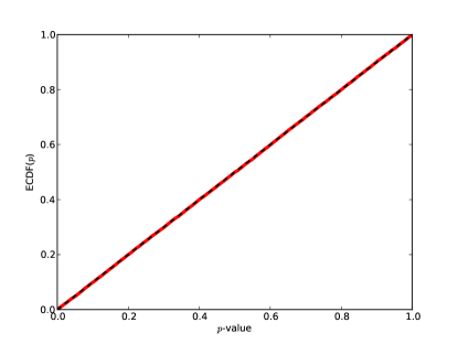
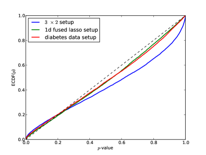
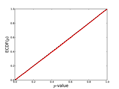
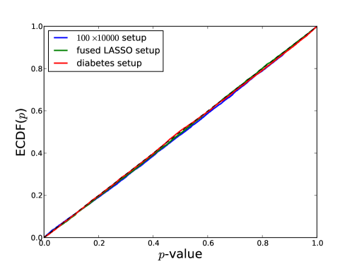
Figure 1(a) shows the empirical distribution function of a sample of 20,000 p-values (6), constructed from lasso problems with a variety of different predictor matrices, all under the global null model . In particular, for each sample, we drew the predictor matrix uniformly at random from the following cases:
-
•
small case: is , with values (in row-major order) equal to ;
-
•
fat case: is , with columns drawn from the compound symmetric Gaussian distribution having correlation 0.5;
-
•
tall case: is , with columns drawn from the compound symmetric Gaussian distribution having correlation 0.5;
-
•
lower triangular case: is , a lower triangular matrix of 1s [the lasso problem here is effectively a reparametrization of the 1-dimensional fused lasso problem (Tibshirani et al., 2005)];
-
•
diabetes data case: is , the diabetes data set studied in Efron et al. (2004).
As is seen in the plot, the agreement with uniform is very strong.
In their proposed covariance test, Lockhart et al. (2013) show that under the global null hypothesis ,
| (8) |
assuming standardized predictors, for , independent errors in (4) with unit marginal variance, , and a condition to ensure that diverges to at a sufficient rate.
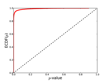
In finite samples, using as an approximation to the distribution of the covariance test statistic seems generally conservative, especially for smaller values of and . Figure 1(b) shows the empirical distribution function from 10,000 covariance test p-values, in three of the above scenarios. [The predictors were standardized before applying the covariance test, in all three cases; this is not necessary, as the covariance test can be adapted to the more general case of unstandardized predictors, but was done for simplicity, to match the form of the test as written in (8).] Even though the idea behind the covariance test can be conceivably extended to other regularized regression problems (outside of the lasso setting), the approximation to its distribution is generally inappropriate, as we will see in later examples. Our test, however, naturally extends to general regularization settings, allowing us to attack problems with more complex penalties such as the group lasso and nuclear norm penalties.
The rest of this paper is organized as follows. In Section 2, we describe the general framework for regularized regression problems that we consider, and a corresponding global null hypothesis of interest; we also state our main result, Theorem 1, which gives an exact p-value for this null hypothesis. The next two sections are then dedicated to proving Theorem 1. Section 3 characterizes the global maximizer (2) in terms of the related Gaussian process and its gradient. Section 4 applies the Kac-Rice formula to derive the joint distribution of the maximum value of the process (1) and its maximizer (2), which is ultimately used to derive the (uniform) distribution of our proposed test. In Section 5 we broadly consider practicalities associated with constructing our test statistic, revisit the lasso problem, and examine the group lasso, principal components, and matrix completion problems as well. Section 6 discusses the details of the computation of the quantities and needed for our main result. We empirically investigate the null distribution of our test statistic under non-Gaussian errors in Section 7, and end with a short discussion in Section 8.
2 General regularized regression problems
We examine a class of regularized least squares problems of the form
| (9) |
with outcome , predictor matrix , and regularization parameter . We assume that the penalty function satisfies
| (10) |
where is a convex set, i.e., is the support function of . This serves as a very general penalty, as we can represent any seminorm (and hence any norm) in this form with the proper choice of set . In this work, we will use the abuse of notation of calling (10) a semi-norm (that is, we do not require symmetry of semi-norms). We note that the solution above is not necessarily unique (depending on the matrix and set ) and the element notation used in (9) reflects this. A standard calculation, which we give in Appendix A.1, shows that the fitted value is always unique, and hence so is .
Now define
This is the smallest value of for which the penalty term in (9) is zero; any smaller value of the tuning parameter returns a non-trivial solution, according to the penalty. A straightforward calculation involving subgradients, which we give in Appendix A.2, shows that
| (11) |
where is the dual seminorm of , i.e., , the support function of the polar set of . This set can be defined as , or equivalently,
the unit ball in . Furthermore, in (11), we use to denote the projection operator onto the linear subspace
We recall that for the lasso problem (3), the penalty function is , so ; also , which means that , and hence , as claimed in Section 1.1.
Having just given an example of a seminorm in which is of full dimension , so that , we now consider one in which has dimension less than , so that is nontrivial. In a generalized lasso problem (Tibshirani & Taylor, 2011), the penalty is for some chosen penalty matrix . In this case, it can be shown that the dual seminorm is . Hence , and , the null space of . In many interesting cases, this null space is nontrivial; e.g., if is the fused lasso penalty matrix, then its null space is spanned by the vector of all 1s. In fact, the usual form of the LASSO Tibshirani (1996) is a seminorm:
Of course, the above problem can be solved by solving
Both of these problems fit into the framework (9).
2.1 A null hypothesis
As in the lasso case, we assume that is generated from the normal model
| (12) |
with considered fixed. We are interested in the distribution of (1) in order to test the following hypothesis:
| (13) |
This can be seen a global null hypothesis, a test of whether the true underlying coefficient vector has a trivial structure, according to the designated penalty function .
Assuming that the set contains 0 in its relative interior, we have , where denotes the projection matrix onto . Therefore we can rewrite the null hypothesis (13) in a more transparent form, as
| (14) |
Again, using the lasso problem (3) as a reference point, we have for this problem, so the above null hypothesis reduces to , as in Section 1.1. In general, the null hypothesis (14) tests , the orthocomplement of .
Recalling that
one can check that, under , the quantity is precisely of the form (1), with , , and [as when ].
2.2 Statement of main result and outline of our approach
We now state our main result.
Theorem 1 (Main result: Kac-Rice test).
Consider the general regularized regression problem in (9), with for a closed, convex set containing 0 in its relative interior. Denote , the polar set of , and assume that can be stratified into pieces of different dimensions, i.e.,
| (15) |
where are smooth disjoint manifolds of dimensions , respectively. Assume also assume that the process
| (16) |
is Morse for almost every . Finally, assume that is drawn from the normal distribution in (12).
Now, consider testing the null hypothesis [equivalently, , since we have assumed that ]. Define for as in (29), (30), as in (24), (23), and as in (32). Finally, let denote the almost sure unique maximizer of the process over ,
and let denote the first knot in the solution path of problem (9). Then under ,
| (17) |
where denotes the density function of a normal random variable with mean 0 and variance .
The quantity (17) is the Kac-Rice pivot evaluated at . Lemma 5 shows it is a pivotal quantity for the mean near , derived via the Kac-Rice formula. Here we give a rough explanation of the result in (17), and the approach we take to prove it in Sections 3 and 4. The next section, Section 2.3, discusses the assumptions behind Theorem 1; in summary, the assumption that separates as in (15) allows us to apply the Kac-Rice formula to each of its strata, and the Morse assumption on the process in (16) ensures the uniqueness of its maximizer . These are very weak assumptions, especially considering the strength of the exact, non-asymptotic conclusion in (17).
Our general approach is based on finding an implicit formula for under the null hypothesis , where is the first knot in the solution path of problem (9) and can be written as
where , the process in (16). Our representation for the tail probability of has the form
| (18) |
Here is a random distribution function, is the indicator function for the interval ), and is a maximizer of the process . This maximizer , almost surely unique by the Morse assumption, satisfies
with the subdifferential of the seminorm . Under the assumption that , the main tool we invoke is the Kac-Rice formula (Adler & Taylor, 2007), which essentially enables us to compute the expected number of global maximizers occuring in each stratum .
Remark 1.
Note that for almost every realization, under the Morse assumption, there is generically only one maximizer overall and hence the number of them is either 0 or 1. We use the term ”number of global maximizers” when applying the Kac-Rice formula as it applies to counting different types of points. In our applications of it, however, there is only ever 0 or 1 such points. Similar arguments were used to establish the accuracy of the expected Euler characteristic approximation for the distribution of the global maximum of a smooth Gaussian process in Taylor et al. (2005).
This leads to the distribution of , in Theorem 2, as well as the representation in (18), with given in an explicit form. Unfortunately, computing tail probabilities of this distribution involve evaluating some complicated integrals over that depend on , and hence the quantity as a test statistic does not easily lend itself to the computation of p-values. We therefore turn to the survival function associated with the measure , and our main result is that, when carefully evaluated, this (random) survival function can be used to derive a test of , as expressed in (17) in Theorem 1 above.
2.3 Discussion of assumptions
In terms of the assumptions of Theorem 1, we require that contains 0 in its relative interior so that we can write the null hypothesis in the equivalent form , which makes the process in (16) have mean zero under . We additionally assume that is closed in order to guarantee that has a well-defined (finite) maximum over . See Appendix A.3.
Apart from these rather minor assumptions on , the main requirements of the theorem are: the polar set can be stratified as in (15), the process in (16) is Morse, and follows the normal distribution in (12). Overall, these are quite weak assumptions. The first assumption, on separating as in (15), eventually permits us to apply to the Kac-Rice formula to each stratum . We remark that many convex (and non-convex) sets possess such a decomposition; see Adler & Taylor (2007). In particular, we note that such an assumption does not limit our consideration to polyhedral : a set can be stratifiable but still have a boundary with curvature (e.g., as in for the group lasso and nuclear norm penalties).
Further, the property of being a Morse function is truly generic; again, see Adler & Taylor (2007) for a discussion of Morse functions on stratified spaces. If is Morse for almost every , then its maximizers are almost surely isolated, and the convexity of then implies that has an almost surely unique maximizer . From the form of our particular process in (16), the assumption that is Morse can be seen as a restriction on the predictor matrix (or more generally, how interacts with the set ). For most problems, this only rules out trivial choices of . In the lasso case, for example, recall that and is equal to the unit ball, so , and the Morse property requires , to be unique for almost every . This can be ensured by taking with columns in general position [a weak condition that also ensures uniqueness of the lasso solution; see Tibshirani (2013)].
Lastly, the assumption of normally distributed errors in the regression model (12) is important for the work that follows in Sections 3 and 4, which is based on Gaussian process theory. Note that we assume a known covariance matrix , but we allow for a dependence between the errors (i.e., need not be diagonal). Empirically, the (uniform) distribution of our test statistic under the null hypothesis appears to quite robust against non-normal errors in many cases of interest; we present such simulation results in Section 7.
2.4 Notation
Rewrite the process in (16) as
where and . The distribution of is hence , where . Furthermore, under the null hypothesis , we have . For convenience, in Sections 3 and 4, we will drop the tilde notation, and write as simply , respectively. To be perfectly explicit, this means that we will write the process in (16) as
where , and the null hypothesis is . Notice that when , we have exactly , since . However, we reiterate that replacing by in Sections 3 and 4 is done purely for notational convenience, and the reader should bear in mind that the arguments themselves do not portray any loss of generality.
We will write to emphasize that an expectation is taken under the null distribution .
3 Characterization of the global maximizer
Near any point , the set is well-approximated by the support cone , which is defined as the polar cone of the normal cone . The support cone contains a largest linear subspace—we will refer to this , the tangent space to at . The tangent space plays an important role in what follows.
Remark 2.
Until Section 6, the convexity of the parameter space is not necessary; we only need local convexity as described in Adler & Taylor (2007), i.e., we only need to assume that the support cone of is locally convex everywhere. This is essentially the same as positive reach (Federer, 1959). To be clear, while convexity is used in connecting the Kac-Rice test to regularized regression problems in (11) (i.e. it establishes an equality between left and right hand sides), the right hand side is well-defined even if the set is not convex. That is, the in (1) need not be convex. In fact, the issue of convexity is only important for computational purposes, not theoretical purposes. In this sense, this work provides an exact conditional test based on the global maximizer of a smooth Gaussian field on a fairly arbitrary set. This is an advance in the theory of smooth Gaussian fields as developed in Adler & Taylor (2007) and will be investigated in future work.
We study the process in (16), which we now write as over , where , and with the null hypothesis (see our notational reduction in Section 2.4). We proceed as in Chapter 14 of Adler & Taylor (2007), with an important difference being that here the process does not have constant variance. Aside from the statistical implications of this work that have to do with hypothesis testing, another goal of this paper is to derive analogues of the results in Taylor et al. (2005); Adler & Taylor (2007) for Gaussian processes with nonconstant variance. For each , we define a modified process
where is the vector that, under , computes the expectation of given , the gradient restricted to , i.e.,
To check that such a representation is possible, suppose that the tangent space is -dimensional, and let be a matrix whose columns form an orthonormal basis for . Then , and a simple calculation using the properties of conditional expectations for jointly Gaussian random variables shows that
where
| (19) |
the projection onto with respect to (and denoting the Moore-Penrose pseudoinverse of a matrix ). Hence, we gather that
and our modified process has the form
| (20) |
The key observation, as in Taylor et al. (2005) and Adler & Taylor (2007), is that if is a critical point, i.e., , then
| (21) |
Similar to our construction of , we define such that
| (22) |
and after making three subsequent definitions,
| (23) | ||||
| (24) | ||||
| (25) |
we are ready to state our characterization of the global maximizer .
Lemma 1.
A point maximizes over a convex set if and only if the following conditions hold:
| (26) |
The same equivalence holds true even when is only locally convex.
Proof.
In the forward direction (), note that implies that we can replace by (and by ) in the definitions (24), (23), (25), by the key observation (21). As each is covered by one of the cases , , , we conclude that
i.e., the point is a global maximizer.
As for the reverse direction (), when is the global maximizer of over , the first condition is clearly true (provided that is convex or locally convex), and the other three conditions follow from simple manipulations of the inequalities
∎
Remark 3.
The above lemma does not assume that decomposes into strata, or that is Morse for almost all , or that . It only assumes that is convex or locally convex, and its conclusion is completely deterministic, depending only on the process via its covariance function under the null, i.e., via the terms and .
We note that, under the assumption that is Morse over for almost every , and is convex, Lemma 1 gives necessary and sufficient conditions for a point to be the almost sure unique global maximizer. Hence, for convex , the conditions in (26) are equivalent to the usual subgradient conditions for optimality, which may be written as
where is the normal cone to at and is the gradient restricted to the orthogonal complement of the tangent space .
Recalling that is a Gaussian process, a helpful independence relationship unfolds.
Lemma 2.
With , for each fixed , the triplet is independent of .
Proof.
This is a basic property of conditional expectation for jointly Gaussian variables, i.e., it is easily verified that for all . ∎
4 Kac-Rice formulae for the global maximizer and its value
The characterization of the global maximizer from the last section, along with the Kac-Rice formula (Adler & Taylor, 2007), allow us to express the joint distribution of
Theorem 2 (Joint distribution of ).
Writing for a stratification of , for open sets ,
| (27) |
where:
-
•
is the density of the gradient in some basis for the tangent space , orthonormal with respect to the standard inner product on , i.e., the standard Euclidean Riemannian metric on ;
-
•
the measure is the Hausdorff measure induced by the above Riemannian metric on each ;
-
•
the Hessian is evaluated in this orthonormal basis and, for , we take as convention the determinant of a matrix to be 1 [in Adler & Taylor (2007), this was denoted by , to emphasize that it is the Hessian of the restriction of to ].
Proof.
This is the Kac-Rice formula, or the “meta-theorem” of Chapter 10 of Adler & Taylor (2007) (see also Azaïs & Wschebor, 2008; Brillinger, 1972), applied to the problem of counting the number of global maximizers in some set having value in . That is,
where the second equality follows from (21). Breaking down into its separate strata, and then using the Kac-Rice formula, we obtain the result in (27). ∎
Remark 4.
As before, the conclusion of Theorem 2 does not actually depend on the convexity of . When is only locally convex, the Kac-Rice formula [i.e., the right-hand side in (27)] counts the expected total number of global maximizers of lying in some set , with the achieved maximum value in . For convex , our Morse condition on implies an almost surely unique maximizer, and hence the notation on the left-hand side of (27) makes sense as written. For locally convex , one simply needs to interpret the left-hand side as
Remark 5.
When has constant variance, the distribution of the maximum value can be approximated extremely well by the expected Euler characteristic (Adler & Taylor, 2007) of the excursion set ,
This approximation is exact when is convex (Takemura & Kuriki, 2002), since the Euler characteristic of the excursion set is equal to the indicator that it is not empty.
4.1 Decomposition of the Hessian
In looking at the formula (27), we note that the quantities inside the indicator are all independent, by construction, of . It will be useful to decompose the Hessian term similarly. We write
where
| (28) | ||||
| (29) | ||||
| (30) |
At a critical point of , notice that (being a linear function of the gradient , which is zero at such a critical point). Furthermore, the pair of matrices is independent of . Hence, we can rewrite our key formulae for the distribution of the maximizer and its value.
Lemma 3.
For each fixed , we have
independently of , with
| (31) | ||||
| (32) |
and (recall) , for an orthonormal basis of .
4.2 The conditional distribution
The Kac-Rice formula can be generalized further. For a possibly random function , with continuous for each , we see as a natural extension from (33),
| (36) |
This allows us to form a conditional distribution function of sorts. As defined in (35), is not a probability measure, but it can be normalized to yield one:
| (37) |
Working form (36), with ,
| (38) |
This brings us to our next result.
Lemma 4.
Formally, the measure is a conditional distribution function of , in the sense that on each stratum , , we have
| (39) |
for all .
Proof.
By expanding the right-hand side in (38), we see
where denotes the joint distribution of at a fixed value of . Consider the quantity
| (40) |
We claim that this is the joint density (modulo differential terms) of , when is restricted to the smooth piece . This would complete the proof. Hence to verify the claim, we the apply Kac-Rice formula with open sets , , and , giving
Taking to be open balls around some fixed points , respectively, and sending their radii to zero, we see that the joint density of , with restricted to , is exactly as in (40), as desired. ∎
Remark 7.
The analogous result also holds unconditionally, i.e., it is clear that
by taking an expectation on both sides of (39).
4.3 The Kac-Rice pivotal quantity
Suppose that we are interested in testing the null hypothesis . We might look at the observed value of the first knot , and see if it was larger than we would expect under . From the results of the last section,
and so the most natural strategy seems to be to plug our observed value of the first knot into the above formula. This, however, requires computing the above expectation, i.e., the integral in (38).
In this section, we present an alternative approach that is effectively a conditional test, conditioning on the observed value of , as well as and . To motivate our test, it helps to take a step back and think about the measure defined in (37). For fixed values of , we can reexpress this (nonrandom) measure as
where is a density function (supported on ). In other words, computes the expectation of with respect to a density , so we can write where is a random variable whose density is . Now consider the survival function
A classic argument shows that . Why is this useful? Well, according to lemma 4 (or, Remark 7 following the lemma), the first knot almost takes the role of above, except that there is a further level of randomness in , and . That is, instead of the expectation of being given by , it is given by . The key intuition is that the random variable
| (41) |
should still be uniformly distributed, since this is true conditional on , and unconditionally, the extra level of randomness in just gets “averaged out” and does not change the distribution. Our next lemma formalizes this intuition, and therefore provides a test for based on the (random) survival function in (41).
Lemma 5.
[Kac-Rice pivot] The survival function of , with , , , , and evaluated at , satisfies
| (42) |
Proof.
Fix some . A standard argument shows that (fixing ),
Now we compute, applying (38) with being a composition of functions,
∎
Remark 8.
Remark 9.
We have used the survival function of conditional on being the global maximizer as well the additional local information . Conditioning on this extra information makes the test very simple to compute, at least in the LASSO, group LASSO and nuclear norm cases. If we were to marginalize over these quantities, we would have a more powerful test. In general, it seems difficult to analytically marginalize over these quantities, but perhaps Monte Carlo schemes would be feasible. Further, Lemma 5 holds for any , implying that this marginalization over would need access to the unknown . Under the global null, , this is not too much of an issue, though it already causes a problem for the construction of selection intervals described in Section 8.2.
5 Practicalities and examples
Given an instance of the regularized regression problem in (9), we seek to compute the test statistic
| (43) |
and compare this against . Recalling that , this leaves us with essentially 6 quantities to be computed——and the above integral to be calculated.
If we know the dual seminorm of the penalty in closed form, then the first knot can be found explicitly, as in ; otherwise, it can be found numerically by solving the (convex) optimization problem
The remaining quantities, , all depend on and on the tangent space . Again, depending on , the maximizer can either be found in closed form, or numerically by solving the above optimization problem. Once we know the projection operator onto the tangent space , there is an explicit expression for , recall (32); furthermore, are given by two more tractable (convex) optimization problems (which in some cases admit closed form solutions), see Section 6.
The quantities are different, however; even once we know and the tangent space , finding involves computing the Hessian , which requires a geometric understanding of the curvature of around . That is, cannot be calculated numerically (say, via an optimization procedure, as with ), and demand a more problem-specific, mathematical focus. For this reason, computation of can end up being an involved process (depending on the problem). In the examples that follow, we do not give derivation details for the Hessian , but refer the reader to Adler & Taylor (2007) for the appropriate background material.
JL – This seemed like a natural spot to include the algorithm
We now revisit the lasso example, and then consider the group lasso and nuclear norm penalties, the latter yielding applications to principal components and matrix completion. We remark that in the lasso and group lasso cases, the matrix is zero, simplifying the computations. In contrast, it is nonzero for the nuclear norm case.
Also, it is important to point out that in all three problem cases, we have , so the notational shortcut that we applied in Sections 3 and 4 has no effect (see Section 2.4), and we can use the formulae from these sections as written.
5.1 Example: the lasso (revisited)
For the lasso problem (3), we have and , so and . Our Morse assumption on the process over (which amounts to an assumption on the design matrix ) implies that there is a unique index such that
Then in this notation (where is the th standard basis vector), and the normal cone to at is
Because this is a full-dimensional set, the tangent space to at is . This greatly simplifies our survival function test statistic (41) since all matrices in consideration here are and therefore have determinant 1, giving
The lower and upper limits are easily computed by solving two linear fractional programs, see Section 6. The variance of is given by (32), and again simplifies because is zero dimensional, becoming
Plugging in this value gives the test statistic as in (6) in Section 1.1. The reader can return to this section for examples and discussion in the lasso case.
5.2 Example: the group lasso
The group lasso (Yuan & Lin, 2006) can be viewed as an extension of the lasso for grouped (rather than individual) variable selection. Given a pre-defined collection of groups, with , the group lasso penalty is defined as
where denotes the subset of components of corresponding to , and for all . We note that
so the dual of the penalty is
and
Under the Morse assumption on over (again, this corresponds to an assumption about the design matrix ), there is a unique group such that
where we write to denote the matrix whose columns are a subset of those of , corresponding to . Then the maximizer is given by
and the normal cone is seen to be
Hence the tangent space is
which has dimension , with . An orthonormal basis for this tangent space is given by padding an orthonormal basis for with zeros appropriately. From this we can compute the projection operator
and the variance of as
The quantities can be readily computed by solving two convex programs, see Section 6. Finally, we have in the group lasso case, as the special form of curvature matrix of a sphere implies that in (29). This makes , and the test statistic (43) for the group lasso problem becomes
| (44) |
In the above, denotes a chi distributed random variable with degrees of freedom, and the equality follows from the fact that the missing multiplicative factor in the density [namely, ] is common to the numerator and denominator, and hence cancels.
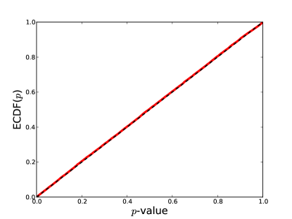
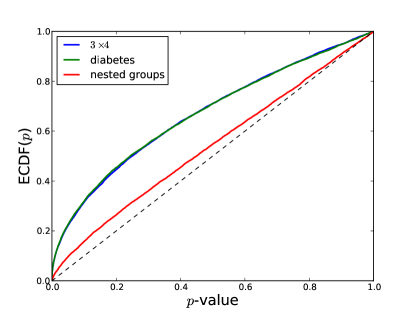
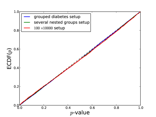
Figure 2(a) shows the empirical distribution function of a sample of 20,000 p-values from problem instances sampled randomly from a variety of different group lasso setups (all under the global null model ):
-
•
small case: is , a fixed matrix slightly perturbed by Gaussian noise; there are 2 groups of size 2, one with weight , the other with weight ;
-
•
fat case: is with features drawn from the compound symmetric Gaussian distribution having correlation 0.5; here are 1000 groups each of size 10, each having weight ;
-
•
tall case: is with features drawn from the compound symmetric Gaussian distribution having correlation 0.5; there are 1000 groups each of size 10, each having weight ;
-
•
square case: is with features drawn from the compound symmetric Gaussian distribution having correlation 0.5; there are 10 groups each of size 10, each having weight ;
-
•
diabetes case 1: is , the diabetes data set from Efron et al. (2004); there are 4 (arbitrarily created) groups: one of size 4, one of size 2, one of size 3 and one of size 1, with varying weights;
-
•
diabetes case 2: is , the diabetes data set from Efron et al. (2004); there are now 10 groups of size 1 with i.i.d. random weights drawn from (generated once for the entire simulation);
-
•
nested case 1: is , with two nested groups (the column space for one group of size 2 is contained in that of the other group of size 8) with the weights favoring inclusion of the larger group first;
-
•
nested case 2: is , with two nested groups (the column space for one group of size 2 is contained in that of the other group of size 8) with the weights favoring inclusion of the smaller group first;
-
•
nested case 3: is , with two sets of two nested groups (in each set, the column space for one group of size 2 is contained in that of the other group of size 4) with the weights chosen according to group size;
-
•
nested case 4: is , with twenty sets of two nested groups (in each set, the column space for one group of size 2 is contained in that of the other group of size 4) with the weights chosen according to group size.
As we can see from the plot, the p-values are extremely close to uniform.
In comparison, arguments similar to those given in Lockhart et al. (2013) for the lasso case would suggest that for the group lasso, under the null hypothesis,
under some conditions (one of these being that diverges to fast enough). Figure 2(b) shows the empirical distribution function of 10,000 samples from three of the above scenarios, demonstrating that, while asymptotically reasonable, the approximation for the covariance test in the group lasso case can be quite anti-conservative in finite samples.
5.3 Nuclear norm
In this setting, we treat the coefficients in (9) as a matrix, instead of a vector, denoted by . We consider a nuclear norm penalty on ,
where is the diagonal matrix of singular values in the singular value decomposition . Here the dual seminorm is
the operator norm (or spectral norm) of , i.e., its maximum singular value. Therefore we have
Examples of problems of the form (9) with nuclear norm penalty can be roughly categorized according to the choice of linear operator . For example,
-
•
principal components analysis: if is the identity map, then is the largest singular value of , and moreover, is the second largest singular value of ;
- •
- •
The first knot in the solution path is given by , with denoting the adjoint of the linear operator . Assuming that has singular value decomposition with for , and that the process is Morse over , there is a unique achieving the value ,
where are the first columns of , respectively. The normal cone is
and so the tangent space is
From this tangent space, the marginal variance in (32) can be easily computed. This leaves to be addressed. As always, the quantities can be determined numerically, as the optimal values of two convex programs, see Section 6. We now discuss computation of the matrices , and refer the reader to Candes et al. (2012); Takemura & Kuriki (2002, 1997) for some of the calculations that follow. The entries of are given by
with as in (22), which has a similar computational form to , and can be computed from knowledge of above. The entries of are given by
When expressed in a suitable ordering of the above basis of the tangent space, the matrix form of the above expressions are, abbreviating ,
where denotes all but the first column of , with similarly defined, and denotes the matrix with zeros added below in such a way that is an matrix. That is, if ,
In the special case of principal components analysis, in which is the identity map on , the above expressions simplify to and
and the eigenvalues of are seen to be
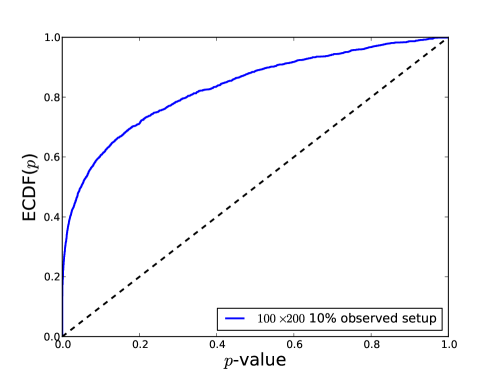
In Figure 3, we plot the empirical distribution function of a sample of 20,000 p-values computed over problem instances that have been randomly sampled from the following scenarios, all employing the nuclear norm penalty (and all under the null model , with being the underlying coefficient matrix):
-
•
principal components analysis: is ;
-
•
matrix completion: is with 50% of its entries observed at random, with 20% of its entries observed at random, with a nonrandom pattern of observed entries, with a nonrandom pattern of observed entries, with 10% of its entries observed at random;
-
•
reduced rank regression: is whose entries are drawn from the compound symmetric Gaussian distribution with correlation 0.5, and is .
As is evident in the plot, the agreement with uniform is excellent (as above, each particular scenario above produces -values regardless of how was chosen, modulo the Morse assumption).
Again, along the lines of the covariance test, we consider approximation of by an distribution under the null hypothesis. Figure 3(b) shows that this approximation is quite far off, certainly much more so than in the other examples. Preliminary calculations confirm mathematically that the distribution is not the right limiting distribution here; we will pursue this in future work.
6 Finding
Earlier, in Remark we noted that convexity of was not needed for much of the work in this paper. It is only when we wish to actually compute the test statistic that we restrict to convex . This section describes convex optimization problems that can be solved to find the values of which are one of the key stumbling pieces to computing the test statistic. Nevertheless, if we had access to a computer that could compute these quantities, along with we would not need to restrict interest to convex . We are still assuming positive reach as this is an important assumption to ensure the modified processes are not singular. See Chapter 14 of Adler & Taylor (2007) for the case when is a smooth locally convex (i.e. positive reach) subset of the Euclidean sphere. This paper considers arbitrary smooth subsets of positive reach up to this point.
Inspecting Lemma 5, we see that in order to compute the -value in (17), we must find at . Recall the definition of in (24),
where is defined as in (22), and can be expressed more concisely as
Recall that at we have for all , and , so
Therefore, is given by the maximization problem
| (45) |
This is a generalized linear-fractional problem (Boyd & Vandenberghe, 2004). (We say “generalized” here because the constraint can be seen as an infinite number of linear constraints, while the standard linear-fractional setup features a finite number of linear constraints.) Though not convex, problem (45) is quasilinear (i.e., both quasiconvex and quasiconcave), and further, it is equivalent to a convex problem. Specifically,
| (46) |
The proof of equivalence between (45) and (46) follows closely Section 4.3.2 of Boyd & Vandenberghe (2004), and so we omit it here. Similarly, is given by the convex minimization problem
| (47) |
In the worst case, and can be determined numerically by solving the problems (46) and (47). Depending on the penalty , one may favor a particular convex optimization routine over another for this task, but a general purpose solver like ADMM (Boyd et al., 2011) should be suitable for a wide variety of penalties. In several special cases involving the lasso, group lasso, and nuclear norm penalties, and have closed-form expressions. We state these next, but in the interest of space, withhold derivation details. We leave more precise calculations to future work.
6.1 Lasso and group lasso
The lasso problem is a special case of the group lasso where all groups have size one; therefore the formulae derived here for the group lasso also apply to the lasso. (In the lasso case, actually, the angles below are always .)
For any group , let be the angle between and [where recall that is as defined in (22)], and define the angles by
Define the quantities
and
Then have the explicitly computable form
6.2 Nuclear norm
For principal components analysis, when , it is not difficult to show that and . Numerically, this seems to be true even for an arbitrary (reduced rank regression) or arbitrary patterns of missingness (matrix completion). We remark that computing requires solving an eigenvalue problem of size at least . (The ADMM approach for solving problem (46) is no better, as each iteration involves projecting onto the nuclear norm epigraph, which requires an eigendecomposition.) This is quite an expensive computation, and a fast approximation is desirable. We leave this for future work.
6.3 Relation to second knot in the solution path
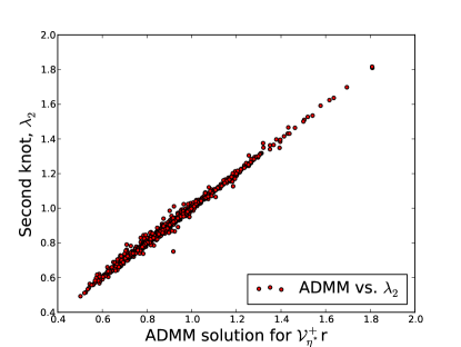
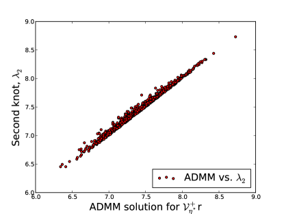
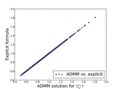
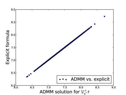
The quantity is always a lower bound on the first knot , and possesses an interesting connection to another tuning parameter value of interest along the solution path. In particular, is related to the second knot , which can be interpreted more precisely in a problem-specific context, as follows:
-
•
for the lasso, with standardized predictors, for all , we have exactly , the value of the tuning parameter at which the solution changes from one nonzero component to two [this follows from a calculation as in Section 4.1 of Lockhart et al. (2013)];
-
•
for the group lasso, as shown in Figure 5(a), is numerically very close to the value of the parameter at which the solution changes from one nonzero group of components to two;
-
•
for the nuclear norm penalty, as shown in Figure 5(b), is numerically very close to the value of the parameter at which the solution changes from rank 1 to rank 2.
7 Non-Gaussian errors
Throughout, our calculations have rather explicitly used the fact that is Gaussian distributed. One could potentially appeal to the central limit theorem if the components of are i.i.d. from some error distribution (treating as fixed), though the calculations in this work focus on the extreme values, so the accuracy of the central limit theorem in the tails may be in doubt. In the interest of space, we do not address this issue here.
Instead, we consider a scenario with heavier tailed, skewed noise and present simulation results. In particular, we drew errors according to a -distribution with 5 degrees of freedom plus an independent centered . Figure 6(c) shows that the lasso and group lasso p-values are relatively well-behaved, while the nuclear norm p-values seem to break down.
8 Discussion
We derived an exact (non-asymptotic) p-value for testing a global null hypothesis in a general regularized regression setting. Our test is based on a geometric characterization of regularized regression estimators and the Kac-Rice formula, and has a close relationship to the covariance test for the lasso problem (Lockhart et al., 2013). In fact, the limiting null distribution of the covariance test can be derived from the formulae given here. These two tests give similar results for lasso problems, but our new test has exact (not asymptotic) error control under the null, with less assumptions on the predictor matrix .
Another strength of our approach is that it provably extends well beyond the lasso problem; in this paper we examine tests for both the group lasso and nuclear norm regularization problems. Still, the test can be applied outside of these settings too, and is limited only by the difficulty in evaluating the p-value in practice (which relies on geometric quantities to be computed).
We recall that the covariance test for the lasso can be applied at any knot along the solution path, to test if the coefficients of the predictors not yet in the current model are all zero. In other words, it can be used to test more refined null hypotheses, not only the global null. We leave the extension of Theorem 1 to this more general testing problem for future work.
8.1 Power
One important issue we have not yet addressed is the power of our tests. While the setting under which our tests are applicable is quite broad (in the lasso problem, the only assumption needed is that have columns in general position), an end user will likely be interested in how powerful our test is.
8.1.1 Lasso
For the lasso case, our test statistic is based on a conditional distribution of [referred to as the Max test in Arias-Castro et al. (2011)]. Therefore, the best one can expect is to have similar results to the Max test in this situation. For general , a simple sufficient condition for full asymptotic power is that the gap must decrease to 0 no faster than . This follows from the Mills’ ratio approximation
We note here that, in principle, by taking sequences of problems the set of limiting distributions for under is effectively the set of all possible distributions for the maximum absolute value of a (separable) centered Gaussian process. This is a huge class, implying that the study of power for such a problem is also a very broad problem. The Kac-Rice test is based on a conditional distribution for the Max test statistic and is applicable for almost all matrices .
The behavior of the Max test has been established for low coherence designs in Arias-Castro et al. (2011), though we emphasize that our test makes no assumption about coherence. In the interest of space, we consider the power of our test to the Max test in the orthonormal design case. While this is a stronger assumption than low coherence, we expect a similar situation to hold in the low coherence setting discussed in . Attempting to prove that these orthogonal results carry over to a low coherence scenario is an interesting problem for future research and is beyond the scope of this paper.
In the orthonormal case, our test statistic reduces in distribution to
where independently for , and are their order statistics in decreasing order.
We first consider the case of finite sparsity and identity design. The simplest possible alternative hypothesis is the 1-sparse case where a single is nonzero. Let and all other . If is some constant greater than 1, then with high probability the first knot will be achieved by . Standard Gaussian tail bounds can be used to upper bound the Kac-Rice pivot and we see that for any the upper bound goes to 0 as , so in this case the test has asymptotic full power at the same threshold as Bonferroni. This is the best possible threshold for asymptotic power against the 1-sparse alternative. Similar statements hold for -sparse alternatives where is considered fixed.
We now consider the sparsity growing with . Following Arias-Castro et al. (2011), we set of the underlying means , to be nonzero and equal to . This is arguably the worst case for our test, which is based on the gap between and . Let ; this is the threshold for non-trivial asymptotic for the Max test. That is, for any , the Max test is asymptotically power powerful (Type I + Type II error ) if the nonzero means have value , and asymptotically powerless (Type I + Type II error or more) if the nonzero means have value .
A fairly straightforward argument based on the spacings calculations in Lockhart et al. (2013), the asymptotic power of the Kac Rice level test is and Type I + Type II error = . As , we recover the full power in the finite sparsity case.
8.1.2 Group lasso
The authors are not aware of literature on the global power of tests such as the group lasso In practice, using the group lasso penalty allows the modeler freedom to favor certain groups by judicious choices of the group weights. Other interesting examples of the group lasso such as glinternet (Lim & Hastie, 2013) generally have widely varying group sizes.
Nevertheless, if we are willing to make simplifying assumptions on group sizes and the designs, then we can say something about power. The simplest thing might be to again assume orthonormal design, with the additional assumption of equal sized groups and weights. In this very specialized setting, questions of power reduce to questions about order statistics of non-central random variables for a fixed group size . These random variables all have similar tail behavior to random variables, with the effective number of observations now being . We therefore expect similar behavior to the Max test if is fixed. Allowing to vary with , or even be random seems an interesting problem to consider, even in the orthonormal design setting. For general without coherence assumptions this seems like a challenging problem indeed.
8.1.3 Nuclear norm
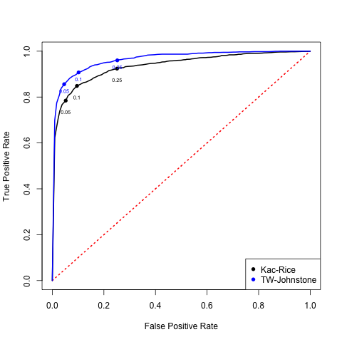
The authors are not aware of other approaches to testing the global null using the test motivated by the nuclear norm, based the largest singular value of . The special case is an obvious exception, in which this largest singular value corresponds to the edge of the spectrum and much is known about the limiting distribution, the Tracy-Widom law Johnstone (2001). In this case, our test statistic is based on the conditional distribution of given . Rather than begin a detailed analysis of the power, we provide a small simulation study to compare to existing implementations based on the Tracy-Widom limit. The simulation is the work of Yunjin Choi, currently a Ph.D. student investigating the use of the Kac-Rice pivot to inference in PCA. The example is a rank-one example, demonstrating that the Kac-Rice test is competitive with the Tracy-Widom approximation of Johnstone (2001). The Kac-Rice test has the advantage of control of Type I error and applicability to the matrix completion or reduced-rank regression setting.
8.2 Related work on selective inference
We conclude this paper with a discussion of how results in this paper can be applied to selective inference and how this paper relates to other recent work. An astute reader will note that all the distributional results in Section 4 are valid for any and not just the global null hypothesis . In this sense, the results in this paper go beyond just hypothesis tests as they can be used to construct intervals containing linear functions of the true mean . Formally, they can be used to construct intervals for defined in (31). Specifically, consider the set
| (48) |
where is defined in (41). As is an exact pivot for we see that
| (49) |
Applying the above to the first step of the lasso, we can construct exact intervals that cover where is the first variable chosen by the lasso. In work initiated after the initial submission of this paper Lee et al. (2013), one of the authors has used this selective inference framework for exact selective inference for selected variables in the problem
| (50) |
for some fixed. With a small modification, one can similarly analyze the problem
| (51) |
In the PCA setting, the above interval gives an interval that covers a pseudo-singular value . If recovered without error, then this would be an actual singular value and the selection interval would be a confidence interval. Under certain conditions for the mean matrix , results in random matrix theory Paul & Johnstone (2012) ensure that the random singular vectors converge in some sense to the population singular vectors, in the sense that . Extending such results to the nuclear norm setting with seems like an interesting and challenging problem.
Perhaps the strongest sense in which these results differ from earlier results on selective inference is that they are exact and computationally feasible. For the lasso, for instance, we need only assume that has columns in general position.
Another sense in which these results differ from existing results on selective inference is that our testing problem allows for the possibility that the choice is made from some continuous set. In the lasso setting, a “mode” is chosen by selecting a set of active variables and their signs. This differs from the group lasso setting in the sense that the active subgradient varies continuously in some set. This added complexity makes conditioning on the “active subgradient” a somewhat more technically dubious procedure. This conditioning is handled explicitly via the Kac-Rice formula which, in this case, can be thought of as enabling us to carry out a partition argument over a smooth partition set.
Finally, the construction of the process is a contribution to the theory of smooth Gaussian random fields as described in Adler & Taylor (2007). Our construction allows earlier proofs that apply only to (centered) Gaussian random fields of constant variance (i.e. marginally stationary) to smooth random fields with arbitrary variance. Even in the marginally stationary case, the conditional distribution defined in (38) provides a new tool for exact selective inference at critical points of such random fields. We leave this, and many other topics, for future work.
Acknowledgements: We are deeply indebted to Robert Tibshirani, without whose help and suggestions this work would not have been possible. Two referees and and an associate editor provided helpful feedback on the first version of this work that has helped the authors improve this paper.
Appendix A Proofs and supplementary details
A.1 Uniqueness of the fitted values and penalty
Consider the strictly convex function . Suppose are two solutions of the regularized problem (9) with . Note
the minimum possible value of the criterion in (9). Define for any . Then by strict convexity of and convexity of ,
contradicting the fact that is the optimal value of the criterion. Therefore we conclude that .
Furthermore, the uniqueness of the fitted value in (9) implies uniqueness of the penalty term , for any .
A.2 Calculation of
By the subgradient optimality conditions, is a solution in (9) if and only if
where denotes the subdifferential (set of subgradients) of evaluated at . Recalling that , we can rewrite this as
| (52) |
The first statement above is equivalent to , where and is the polar body of . Now define
where denotes projection onto the linear subspace
Then for any , the conditions in (52) are satisfied by taking , and accordingly, .
On the other hand, if , then we must have , because implies that , in fact , so and the first condition in (52) is not satisfied.
A.3 Bounded support function
We first establish a technical lemma.
Lemma 6.
Suppose that has . Then for all ,
for some constant , with the polar body of . In other words, is a bounded set.
Proof.
By assumption, we know that for some , where is the projection matrix onto , and is the ball of radius centered at 0. Fix , and define , the boundary of the projected ball of radius . Then for any , we can define , and we have with , hence . As this holds for all , we must have
This implies that , which gives the result. ∎
We now use Lemma 6 to show that the process in (16) is bounded over , assuming that is closed and contains 0 in its relative interior.
Lemma 7.
Proof.
We reparametrize as
and apply Lemma 6 to the process , with , the inverse image of under the linear map . It is straightforward to check, using the fact that is closed, convex, and contains 0 (i.e., using ), that . By Lemma 6, therefore, we know that for all . The proof is completed by noting that , which means for any . ∎
References
- (1)
- Adler & Taylor (2007) Adler, R. J. & Taylor, J. E. (2007), Random fields and geometry, Springer Monographs in Mathematics, Springer, New York.
-
Arias-Castro et al. (2011)
Arias-Castro, E., Candès, E. J. & Plan, Y. (2011), ‘Global testing under sparse alternatives: ANOVA,
multiple comparisons and the higher criticism’, The Annals of
Statistics 39(5), 2533–2556.
Zentralblatt MATH identifier1231.62136.
http://projecteuclid.org/euclid.aos/1322663467 - Azaïs & Wschebor (2008) Azaïs, J.-M. & Wschebor, M. (2008), ‘A general expression for the distribution of the maximum of a Gaussian field and the approximation of the tail’, Stochastic Processes and their Applications 118(7), 1190–1218.
- Boyd et al. (2011) Boyd, S., Parikh, N., Chu, E., Peleato, B. & Eckstein, J. (2011), ‘Distributed optimization and statistical learning via the alternative direction method of multipliers’, Foundations and Trends in Machine Learning 3(1), 1–122.
- Boyd & Vandenberghe (2004) Boyd, S. & Vandenberghe, L. (2004), Convex Optimization, Cambridge University Press, Cambridge.
- Brillinger (1972) Brillinger, D. R. (1972), ‘On the number of solutions of systems of random equations’, Annals of Mathematical Statistics 43(2), 534–540.
- Candés & Recht (2009) Candés, E. & Recht, B. (2009), ‘Exact matrix completion via convex optimization’, Foundations of Computational Mathematics 9(6), 717–772.
- Candes et al. (2012) Candes, E., Sing-Long, C. & Trzasko, J. (2012), ‘Unbiased risk estimates for singular value thresholding and spectral estimators’, arXiv: 1210.4139 .
- Efron et al. (2004) Efron, B., Hastie, T., Johnstone, I. & Tibshirani, R. (2004), ‘Least angle regression’, Annals of Statistics 32(2), 407–499.
- Federer (1959) Federer, H. (1959), ‘Curvature measures’, Transactions of the American Mathematical Society 93(3), 418–491.
- Johnstone (2001) Johnstone, I. M. (2001), ‘On the distribution of the largest eigenvalue in principal components analysis’, The Annals of Statistics 29(2), 295–327.
-
Lee et al. (2013)
Lee, J. D., Sun, D. L., Sun, Y. & Taylor, J. E. (2013), ‘Exact post-selection inference with the lasso’, arXiv:1311.6238 [math, stat] .
http://arxiv.org/abs/1311.6238 -
Lim & Hastie (2013)
Lim, M. & Hastie, T. (2013),
‘Learning interactions through hierarchical group-lasso regularization’, arXiv:1308.2719 [stat] .
http://arxiv.org/abs/1308.2719 - Lockhart et al. (2013) Lockhart, R., Taylor, J. E., Tibshirani, R. J. & Tibshirani, R. (2013), ‘A significance test for the lasso’, arXiv: 1301.7161 .
- Mazumder et al. (2010) Mazumder, R., Hastie, T. & Tibshirani, R. (2010), ‘Spectral regularization algorithms for learning large incomplete matrices’, Journal of machine learning research 11, 2287–2322.
- Mukherjee et al. (2012) Mukherjee, A., Chen, K., Wang, N. & Zhu, J. (2012), ‘On The Degrees of Freedom of Reduced-rank Estimators in Multivariate Regression’, arXiv: 1210.2464 .
-
Paul & Johnstone (2012)
Paul, D. & Johnstone, I. M. (2012), ‘Augmented sparse principal component analysis for high dimensional data’,
arXiv:1202.1242 [math, stat] .
http://arxiv.org/abs/1202.1242 - Takemura & Kuriki (1997) Takemura, A. & Kuriki, S. (1997), ‘Weights of distribution for smooth or piecewise smooth cone alternatives’, Annals of Statistics 25(6), 2368–2387.
- Takemura & Kuriki (2002) Takemura, A. & Kuriki, S. (2002), ‘On the equivalence of the tube and Euler characteristic methods for the distribution of the maximum of Gaussian fields over piecewise smooth domains’, Annals of Applied Probabilitiy 12(2), 768–796.
- Taylor (2013) Taylor, J. E. (2013), ‘The geometry of least squares in the 21st century’, Bernoulli . To appear.
- Taylor et al. (2005) Taylor, J. E., Takemura, A. & Adler, R. J. (2005), ‘Validity of the expected euler characteristic heuristic’, Annals of Probability 33(4), 1362–1396.
- Tibshirani (1996) Tibshirani, R. (1996), ‘Regression shrinkage and selection via the lasso’, Journal of the Royal Statistical Society: Series B 58(1), 267–288.
- Tibshirani (2013) Tibshirani, R. J. (2013), ‘The lasso problem and uniqueness’, Electronic Journal of Statistics 7, 1456–1490.
-
Tibshirani & Taylor (2011)
Tibshirani, R. J. & Taylor, J. (2011), ‘The solution path of the generalized lasso’, The Annals of Statistics 39(3), 1335–1371.
http://projecteuclid.org/euclid.aos/1304514656 - Tibshirani et al. (2005) Tibshirani, R., Saunders, M., Rosset, S., Zhu, J. & Knight, K. (2005), ‘Sparsity and smoothness via the fused lasso’, Journal of the Royal Statistical Society: Series B 67(1), 91–108.
- Yuan & Lin (2006) Yuan, M. & Lin, Y. (2006), ‘Model selection and estimation in regression with grouped variables’, Journal of the Royal Statistical Society: Series B 68(1), 49–67.