Negative Off-Diagonal Conductivities in a Weakly Coupled Quark Gluon Plasma

Abstract

We calculate the conductivity matrix of a weakly coupled quark-gluon plasma at the leading-log order. By setting all quark chemical potentials to be identical, the diagonal conductivities become degenerate and positive, while the off-diagonal ones become degenerate but negative (or zero when the chemical potential vanishes). This means a potential gradient of a certain fermion flavor can drive backward currents of other flavors. A simple explanation is provided for this seemingly counter intuitive phenomenon. It is speculated that this phenomenon is generic and most easily measured in cold atom experiments.

I Introduction

Hydrodynamics describes the evolution of a fluid perturbed away from thermal equilibrium by long wave length fluctuations. The long wave length physics (long compared with the mean field path of particle collisions) can be systematically described by an expansion of space-time derivatives on classical fields with prefactors called transport coefficients. These transport coefficients encode the physics of short (compared with the mean free path) distance and are inputs to hydrodynamics. But they can be computed, in principle, once the microscopic theory of the system is known.

We are interested in computing the transport coefficients in Quantum Chromodynamics (QCD) with $N_{f}$ flavors of massless quarks at finite temperature ($T$) and chemical potentials ($\mu_{a}$, $a=1,2,\cdots,N_{f}$). The leading transport coefficients at the first derivative order include the shear viscosity ($\eta$), bulk viscosity ($\zeta$), and the conductivity matrix ($\lambda$).

The shear viscosity of QCD has attracted a lot of attention recently. Its ratio with the entropy density ($s$) extracted from the hot and dense matter created at Relativistic Heavy Ion Collider (RHIC) Arsene:2004fa ; Adcox:2004mh ; Back:2004je ; Adams:2005dq just above the phase transition temperature ($T_{c}$) yields $1/(4\pi)\leq\eta/s\leq 2.5/(4\pi)$ at $T_{c}\leq T\leq 2T_{c}$ Song:2010mg , which is close to a conjectured universal lower bound of $1/(4\pi)$ Kovtun:2004de inspired by the gauge/gravity duality Maldacena:1997re ; Gubser:1998bc ; Witten:1998qj . This value of $\eta/s$ cannot be explained by extrapolating perturbative QCD result Arnold:2000dr ; Arnold:2003zc ; Chen:2010xk ; Chen:2011km . The smallest $\eta/s$ is likely to exist near $T_{c}$ Csernai:2006zz ; Chen:2006iga (see, e.g., Ref. Chen:2011km for a compilation and more references). Also finite $\mu$ results suggests that $\eta/s$ is smaller at smaller $\mu$. This is based on results of perturbative QCD at $T\gg$ $T_{c}$ Chen:2012jc and of a hadronic gas at $T\ll$ $T_{c}$ and small $\mu$ Chen:2007xe . It is speculated that the same pattern will persist at $T_{c}$ such that the smallest $\eta/s$ might exist near $T_{c}$ with $\mu=0$ Chen:2012jc .

For the bulk viscosity, the sum rule study Kharzeev:2007wb ; Karsch:2007jc shows that $\zeta$ increases rapidly near $T_{c}$ when $T$ approaches $T_{c}$ from above. This is consistent with the lattice gluon plasma result near $T_{c}$ Meyer:2010ii and perturbative QCD result Arnold:2006fz at much higher $T$. This, when combined with pion gas results below $T_{c}$ Chen:2007kx ; FernandezFraile:2008vu ; Lu:2011df ; Dobado:2011qu ; Chakraborty:2010fr , suggests that $\zeta/s$ has a local maximum near $T_{c}$ (see, e.g., Chen:2011km for a compilation). Unlike $\eta/s$, perturbative QCD result shows very small $\mu$ dependence in $\zeta/s$ Chen:2012jc . Note that at high $\mu$, there are also bulk viscosities governed by the weak interaction such as the Urca processes which have consequences in neutron star physics Dong:2007mb ; Alford:2006gy ; Alford:2008pb ; Sa'd:2006qv ; Sa'd:2007ud ; Wang:2010ydb . These are quite different from the transport coefficients from the strong interaction mentioned above.

The perturbative QCD calculations of $\eta$ and $\zeta$ with finite $\mu$ were performed at the leading-log (LL) order of the strong coupling constant ($g$) expansion in Ref. Chen:2012jc . Either $T$ or $\mu$ in the calculation is much larger than $\Lambda_{QCD}$ which is the scale where QCD becomes non-perturbative. But the calculation is not applicable to the color superconducting phase at $\mu/T\rightarrow\infty$, since the vacuum in the calculation has no symmetry breaking.

In this work, we apply the same perturbative QCD approach to compute the conductivity matrix $\lambda$ at the LL order. The conductivity is an important transport coefficient which plays an essential role in the evolution of electromagnetic fields in heavy ion collisions Huang:2013iia ; McLerran:2013hla . The conductivity in strongly coupled quark gluon plasma was calculated with lattice QCD Ding:2010ga ; Amato:2013naa and Dyson-Schwinger equation Qin:2013aaa .

We first review the constraints from the second law of thermal dynamics (i.e. the entropy production should be non-negative) which show that the particle diffusion, heat conductivities, and electric conductivity are all unified into one single conductivity in this system. When $N_{f}>1$, the conductivity becomes a $N_{f}\times N_{f}$ matrix. We then show through the Boltzmann equation that the conductivity matrix $\lambda$ at the LL order is symmetric and positive definite ($\sum_{a,b}\lambda_{ab}X^{a}X^{b}>0$ for any real, non-vanishing vector $X$). The former is a manifestation of the Onsager relation while the latter is a manifestation of the second law of thermal dynamics.

For simplicity, we show the numerical results of $\lambda$ with all fermion chemical potential to be identical. In this limit, there are only two independent entries in $\lambda$. All the diagonal matrix elements are degenerate and positive since $\lambda$ is positive definite. However, the off-diagonal matrix elements are degenerate but negative at finite $\mu$. This means a gradient $\bm{\nabla}\mu_{a}$ can drive a current of flavor $a$ alone the gradient direction, but it will also drive currents of different flavors in the opposite direction. This backward current phenomenon might seem counter intuitive, but we find that it is generic and it has a simple explanation. We speculate that this phenomenon might be most easily measured in cold atom experiments.

II Entropy principle in hydrodynamics

II.1 Single flavor case

Let us start from the hydrodynamical system with only one flavor of quark of electric charge $Q$. The energy-momentum conservation and current conservation yield

$$\partial_{\mu}T^{\mu\nu} =QF^{\nu\lambda}j_{\lambda},$$

$$\partial_{\mu}j^{\mu} =0,$$ (1)

where $T^{\mu\nu}$ is the energy-momentum tensor, $j^{\mu}$ is the quark current and $F^{\nu\lambda}$ is the electromagnetic field strength tensor. The long wave length physics can be systematically described by the expansion of space-time derivatives

$$T^{\mu\nu} =T_{(0)}^{\mu\nu}+\varepsilon T_{(1)}^{\mu\nu}+\varepsilon^{2}T_{(2)}^{\mu\nu}+\cdots,$$

$$j^{\mu} =j_{(0)}^{\mu}+\varepsilon j_{(1)}^{\mu}+\varepsilon^{2}j_{(2)}^{\mu}+\cdots,$$ (2)

where we have used the parameter $\varepsilon$ to keep track of the expansion and we will set $\varepsilon=1$ at the end. $F^{\nu\lambda}$ is counted as $\mathcal{O}(\varepsilon)$. We will then assume the system is isotropic and homogeneous in thermal equilibrium so there is no special directions or intrinsic length scales macroscopically. We also assume the underlying microscopic theory satisfies parity, charge conjugation and time reversal symmetries such that the antisymmetric tensor $\varepsilon^{\mu\nu\alpha\beta}$ does not contribute to $T^{\mu\nu}$ and $j^{\mu}$. Also, we assume the system is fluid-like, describable by one (and only one) velocity field (the conserved charged is assumed to be not broken spontaneously, otherwise the superfluid velocity needs to be introduced as well). Also, at $\mathcal{O}(\varepsilon^{0})$, the system is in local thermal equilibrium, i.e. the system is in equilibrium in the comoving frame where the fluid velocity is zero. With these assumptions, we can parametrize

$$T_{(0)}^{\mu\nu} =\left(\epsilon+P\right)u^{\mu}u^{\nu}-Pg^{\mu\nu},$$

$$j_{(0)}^{\mu} =nu^{\mu},$$

$$T_{(1)}^{\mu\nu} =\Pi\left(u^{\mu}u^{\nu}-g^{\mu\nu}\right)+\pi^{\mu\nu}+h^{\mu}u^{\nu}+h^{\nu}u^{\mu},$$

$$j_{(1)}^{\mu} =\nu^{\mu},$$ (3)

where $g^{\mu\nu}=$diag($+,-,-,-$ ) and $\epsilon$, $P$ and $n$ are the energy density, pressure and number density, respectively. The fluid velocity $u^{\mu}=(u^{0},\bm{u})=(1,\bm{v})/\sqrt{1-\bm{v}^{2}}$ and $u^{\mu}u_{\mu}=1.$ $\Pi$, $\pi^{\mu\nu}$, $h^{\mu}$ and $\nu^{\mu}$ are the bulk viscous pressure, shear viscous tensor, heat flow vector and diffusion current. They satisfy the orthogonal relations, $\pi^{\mu\nu}u_{\nu}=\nu^{\mu}u_{\mu}=h^{\mu}u_{\mu}=0$.

The covariant entropy flow is given by Israel:1979wp ; Pu:2011vr

$$S^{\mu}=\beta Pu^{\mu}+\beta T^{\mu\nu}u_{\nu}-\beta\mu j^{\mu}=su^{\mu}+\beta h^{\mu}-\beta\mu\nu^{\mu},$$ (4)

where $\beta=1/T$ and $s=\beta(\epsilon+P-\mu n)$ is the entropy density. Taking the space-time derivative of $S^{\mu}$, then using the Gibbs-Duhem relation $d\epsilon=Tds+\mu dn$ and the conservation equations (1), we obtain the equation for entropy production:

$$\partial_{\mu}S^{\mu} =-\nu^{\mu}\left[\partial_{\mu}(\beta\mu)+\beta QE_{\mu}\right]+h^{\mu}\left(\partial_{\mu}\beta+\beta u^{\nu}\partial_{\nu}u_{\mu}\right)$$

$$+\beta\pi^{\mu\nu}\partial_{\langle\mu}u_{\nu\rangle}-\beta\Pi\partial\cdot u,$$ (5)

where the symmetric traceless tensor $\partial_{\langle\mu}u_{\nu\rangle}$ is defined by,

$$\partial_{\langle\mu}u_{\nu\rangle}=\frac{1}{2}\left[\Delta_{\mu\alpha}\Delta_{\nu\beta}+\Delta_{\nu\alpha}\Delta_{\mu\beta}-\frac{2}{3}\Delta_{\mu\nu}\Delta_{\alpha\beta}\right]\partial^{\alpha}u^{\beta},$$ (6)

and where$\;\Delta^{\mu\nu}=g^{\mu\nu}-u^{\mu}u^{\nu}$ and $E^{\mu}\equiv F^{\mu\nu}u_{\nu}$ is the electric field in the comoving frame.

At $\mathcal{O}(\varepsilon)$, $\partial_{\mu}T^{\mu\nu}\simeq\partial_{\mu}T_{(0)}^{\mu\nu}=0$. This equation yields

$$\partial_{\mu}\beta+\beta u^{\nu}\partial_{\nu}u_{\mu}=\frac{n}{\epsilon+P}[\partial_{\mu}(\beta\mu)+\beta QE_{\mu}],$$ (7)

where we have used the thermodynamic equation $dP=\beta(\epsilon+P)dT+nTd(\beta\mu)$. This identity simplifies Eq. (5) to

$$\partial_{\mu}S^{\mu} =-\left(\nu^{\mu}-\frac{n}{\epsilon+P}h^{\mu}\right)[\partial_{\mu}(\beta\mu)+\beta QE_{\mu}]$$

$$+\beta\pi^{\mu\nu}\partial_{\left\langle\mu\right.}u_{\left.\nu\right\rangle}-\beta\Pi\partial\cdot u.$$ (8)

The second law of thermodynamics requires $\partial_{\mu}S^{\mu}\geq 0$. It can be satisfied if, up to terms orthogonal to $\partial\cdot u$, $\partial_{\left\langle\mu\right.}u_{\left.\nu\right\rangle}$ and $[\partial_{\mu}(\beta\mu)+\beta QE_{\mu}]$, $\Pi$, $\pi^{\mu\nu}$, $h^{\mu}$ and $\nu^{\mu}$ have the following forms at $\mathcal{O}(\varepsilon)$:

$$\pi^{\mu\nu} =2\eta\partial^{\left\langle\mu\right.}u^{\left.\nu\right\rangle},$$

$$\Pi =-\zeta\partial\cdot u,$$

$$\nu^{\mu}-\frac{n}{\epsilon+P}h^{\mu} =\lambda\Delta^{\mu\nu}\left[\partial_{\nu}(\beta\mu)+\beta QE_{\nu}\right],$$ (9)

where $\Delta^{\mu\nu}$ is inserted because $\nu^{\mu}u_{\mu}=h^{\mu}u_{\mu}=0$. The coefficients $\eta$, $\zeta$ and $\lambda$ are transport coefficients with names of shear viscosity, bulk viscosity and conductivity, respectively. The second law of thermodynamics requires these transport coefficients to be non-negative.

On the right hand side of Eq. (9), the three vectors $\partial_{\nu}\mu$, $\partial_{\nu}\beta$ and $E_{\nu}$ form a unique combination and share the same transport coefficient $\lambda$ Israel:1979wp . It is obtained by assuming $\partial_{\mu}T_{(0)}^{\mu\nu}=0$ and $T_{(0)}^{\mu\nu}$ has the ideal fluid form described in Eq.(3). In general, we do not expect this to be true in all systems (e.g. a solid might not have the ideal fluid description) and hence there could be more transport coefficients. Conventionally, the transport coefficients corresponding to $\partial_{\nu}\mu$, $\partial_{\nu}\beta$ and $E_{\nu}$ are called particle diffusion, heat conductivity, and electric conductivity, respectively.

In hydrodynamics, the choice of the velocity field is not unique. One could choose $\mathbf{u}$ to align with the momentum density $T^{0i}\mathbf{\hat{i}}$ or the current $\mathbf{j}$, or their combinations. However, the system should be invariant under the transformation $u_{\mu}\rightarrow u_{\mu}^{{}^{\prime}}=u_{\mu}+\varepsilon\delta u_{\mu}$ as long as $u_{\mu}^{{}^{\prime}2}=1$ is maintained (or $u^{\mu}\delta u_{\mu}=0$ at $\mathcal{O}(\varepsilon)$). Under this transformation, $h_{\mu}\rightarrow$ $h_{\mu}^{\prime}=h_{\mu}+\left(\epsilon+P\right)\delta u_{\mu}$ and $\nu_{\mu}\rightarrow$ $\nu_{\mu}^{\prime}=\nu_{\mu}+n\delta u_{\mu}$. However, the entropy production equation (8) remains invariant under this transformation.

In this paper, we will be working at the Landau frame with $\mathbf{u}$ proportional to the momentum density $T^{0i}\mathbf{\hat{i}}$ such that $T^{0i}=0$ in the comoving frame. Then

$$\mathbf{h}=0,\quad\bm{\nu}=\lambda[-\bm{\nabla}(\beta\mu)+\beta Q\mathbf{E}]$$ (10)

from Eq. (9). $\lambda$ is positive, the sign makes sense for particle diffusion and electric conduction because the diffusion is from high to low density and positively charged particles move along the $\mathbf{E}$ direction. However, heat conduction induces a flow from low to high temperature! This result is counter intuitive. This is because $\bm{\nabla}T$ induces a momentum flow $\mathbf{h}$. If we choose to boost the system to the Landau frame where $\mathbf{h}=0$, then the physics is less transparent. For particle diffusion and electric conduction this is not a problem, because one could have particles and antiparticles moving in opposite directions and still keep the net momentum flow zero.

The physics of heat conduction becomes clear in the Eckart frame where $\mathbf{u}$ is proportional to the current $\mathbf{j}$ and we have

$$\bm{\nu}=0,\quad\mathbf{h}=-\frac{\epsilon+P}{n}\lambda[-\bm{\nabla}(\beta\mu)+\beta Q\mathbf{E}].$$ (11)

In this frame, the direction of heat conduction is correct (while the physics of particle diffusion and electric conduction become less transparent). As expected, $\mathbf{h}$ stays finite when $\mu=Q=0$ but $\bm{\nabla}\beta\neq 0$.

II.2 Multi-flavor case

When the flavor of massless quarks is increased to $N_{f}$, then there are $N_{f}$ conserved currents $j_{a}^{\mu}$ (the conserved electric current is just a combination of them). The hydrodynamical equations becomes

$$\partial_{\mu}T^{\mu\nu} =\sum_{a=1}^{N_{f}}Q_{a}F^{\nu\lambda}j_{a,\lambda},$$

$$\partial_{\mu}j_{a}^{\mu} =0,\ a=1,2,\cdots,N_{f}.$$ (12)

Then the entropy production yields

$$\partial_{\mu}S^{\mu} = -\sum_{a=1}^{N_{f}}\left(\nu_{a}^{\mu}-\frac{n_{a}}{\epsilon+P}h^{\mu}\right)\left[\partial_{\mu}(\beta\mu_{a})+\beta Q_{a}E_{\mu}\right]+\beta\pi^{\mu\nu}\partial_{\left\langle\mu\right.}u_{\left.\nu\right\rangle}-\beta\Pi\partial\cdot u$$ (13)

$$\geq 0$$

Working in the Landau frame, we have

$$\bm{\nu}_{a}=\sum_{b=1}^{N_{f}}\lambda_{ab}[-\bm{\nabla}(\beta\mu_{b})+\beta Q_{b}\mathbf{E}].$$ (14)

Our task is to compute the $\lambda$ matrix which can be achieved by setting $\bm{\nabla}(\beta\mu_{b})\neq 0$ but $\mathbf{E}=0$. The second law of thermodynamics dictates $\lambda$ being a positive definite matrix.

III Effective kinetic theory

We will use the Boltzmann equation to compute our LL result of $\lambda$. It has been shown that Boltzmann equation gives the same leading order result as the Kubo formula in the coupling constant expansion in a weakly coupled $\phi^{4}$ theory Jeon:1994if ; Hidaka:2010gh and in hot QED Gagnon:2007qt , provided the leading $T$ and $\mu$ dependence in particle masses and scattering amplitudes are included. This conclusion is expected to hold in perturbative QCD as well Arnold:2002zm .

The Boltzmann equation of a quark gluon plasma describes the evolution of the color and spin averaged distribution function $\tilde{f}_{p}^{i}(x)$ for particle $i$ ($i=g,q_{a},\bar{q}_{a}$ with $a=1.2...N_{f}$ for gluon, $N_{f}$ quarks and $N_{f}$ anti-quarks):

$$\frac{d\tilde{f}_{p}^{i}(x)}{dt}=\mathcal{\tilde{C}}_{i},$$ (15)

where $\tilde{f}_{p}^{i}(x)$ is a function of space-time $x^{\mu}=(t,\mathbf{x})$ and momentum $p^{\mu}=(E_{p},\mathbf{p})$.

For the LL calculation, we only need to consider two-particle scattering processes denoted as $c_{1}c_{2}\rightarrow c_{3}c_{4}$. The collision term has the form

$$C_{c_{1}c_{2}\rightarrow c_{3}c_{4}}\equiv\int_{k_{1}k_{2}k_{3}}d\Gamma_{c_{1}c_{2}\rightarrow c_{3}c_{4}}\left[\tilde{f}_{k_{1}}^{c_{1}}\tilde{f}_{k_{2}}^{c_{2}}\tilde{F}_{p}^{c_{3}}\tilde{F}_{k_{3}}^{c_{4}}-\tilde{F}_{k_{1}}^{c_{1}}\tilde{F}_{k_{2}}^{c_{2}}\tilde{f}_{p}^{c_{3}}\tilde{f}_{k_{3}}^{c_{4}}\right].$$ (16)

where $\tilde{F}^{g}=1+\tilde{f}^{g}$ and $\tilde{F}^{q(\bar{q})}=1-\tilde{f}^{q(\bar{q})}$ and

$$d\Gamma_{c_{1}c_{2}\rightarrow c_{3}c_{4}}=\frac{1}{2E_{p}}|M_{c_{1}c_{2}\rightarrow c_{3}c_{4}}|^{2}\prod\limits_{i=1}^{3}\frac{d^{3}k_{i}}{(2\pi)^{3}2E_{k_{i}}}(2\pi)^{4}\delta^{(4)}(k_{1}+k_{2}-k_{3}-p),$$ (17)

where $|M_{c_{1}c_{2}\rightarrow c_{3}c_{4}}|^{2}$ is the matrix element squared with all colors and helicities of the initial and final states summed over. The scattering amplitudes can be regularized by hard thermal loop propagators and in this paper we use the same scattering amplitudes as in Ref. Arnold:2003zc (see also Table I of Ref. Chen:2012jc ). Then the collision term for a quark of flavor $a$ is

$$N_{q}\mathcal{\tilde{C}}_{q_{a}} =\frac{1}{2}C_{q_{a}q_{a}\leftrightarrow q_{a}q_{a}}+C_{q_{a}\bar{q}_{a}\leftrightarrow q_{a}\bar{q}_{a}}+\frac{1}{2}C_{gg\leftrightarrow q_{a}\bar{q}_{a}}+C_{q_{a}g\leftrightarrow q_{a}g}$$

$$+\sum\limits_{b,b\neq a}^{N_{f}-1}(C_{q_{a}q_{b}\leftrightarrow q_{a}q_{b}}+C_{q_{a}\bar{q}_{b}\leftrightarrow q_{a}\bar{q}_{b}}+C_{q_{b}\bar{q}_{b}\leftrightarrow q_{a}\bar{q}_{a}}),$$ (18)

where $N_{q}=2\times 3=6$ is the quark helicity and color degeneracy factor and the factor $1/2$ is included when the initial state is formed by two identical particles. Similarly,

$$N_{g}\mathcal{\tilde{C}}_{g}=\frac{1}{2}C_{gg\leftrightarrow gg}+\sum\limits_{a=1}^{N_{f}}(C_{gq_{a}\leftrightarrow gq_{a}}+C_{g\bar{q}_{a}\leftrightarrow g\bar{q}_{a}}+C_{q_{a}\bar{q}_{a}\leftrightarrow gg}),$$ (19)

where $N_{g}=2\times 8=16$ is the gluon helicity and color degeneracy factor. In equilibrium, the distributions are denoted as $f^{q_{a}(\bar{q}_{a})}$ and $f^{g}$, with

$$f_{p}^{g} =\frac{1}{e^{u\cdot p/T}-1},$$ (20)

$$f_{p}^{q_{a}(\bar{q}_{a})} =\frac{1}{e^{(u\cdot p\mp\mu_{a})/T}+1},$$ (21)

where $T$ is the temperature, $u$ is the fluid four velocity and $\mu_{a}$ is the chemical potential for the quark of flavor $a$. They are all space time dependent.

The thermal masses of gluon and quark/anti-quark for external states (the asymptotic masses) can be computed via Arnold:2002zm ; Mrowczynski:2000ed

$$m_{g}^{2} =\sum_{i}N_{i}C_{i}\frac{2g^{2}}{d_{A}}\int\frac{d^{3}p}{(2\pi)^{3}2E_{p}}f_{p}^{i},$$ (22)

$$m_{q}^{2} =m_{\bar{q}}^{2}=2C_{F}g^{2}\int\frac{d^{3}p}{(2\pi)^{3}2E_{p}}(2f_{p}^{g}+f_{p}^{q}+f_{p}^{\bar{q}}),$$ (23)

where $d_{A}=8$, $C_{g}=C_{A}=3$, and $C_{q(\bar{q})}=C_{F}=4/3$. This yields

$$m_{g}^{2} =\frac{C_{A}}{6}g^{2}T^{2}+\sum_{a=1}^{N_{f}}\frac{C_{F}}{16}g^{2}(T^{2}+\frac{3}{\pi^{2}}\mu_{a}^{2}),$$ (24)

$$m_{q_{a}}^{2} =\frac{1}{4}C_{F}g^{2}\left(T^{2}+\frac{\mu_{a}^{2}}{\pi^{2}}\right),$$ (25)

where we have set $E_{p}=|\mathbf{p}|$ in the integrals on the right hand sides of Eqs. (22) and (23). The difference from non-vanishing masses is of higher order. In this work, we only need the fact that the thermal masses are proportional to $g^{2}$ for the LL results.

III.1 Linearized Boltzmann equation

Matching to the derivative expansion in hydrodynamics, we expand the distribution function of particle $i$ as a local equilibrium distribution plus a correction

$$\tilde{f}_{p}^{i}(x)=f_{p}^{i}-\varepsilon f_{p}^{i}(1\mp f_{p}^{i})\chi^{i},$$ (26)

where the upper/lower sign corresponds to the femion/boson distribution. Inserting Eq. (26) into Eq. (15), we can solve the linearized Boltzmann equation by keeping linear terms in space-time derivatives. Here we neglect the viscous terms related to $\partial_{\mu}u_{\nu}$ in $\chi^{i}$ and consider only the $\bm{\nabla}(\beta\mu_{a})$ terms.

At the zeroth order, $\mathcal{O}(\varepsilon^{0})$, the system is in local thermal equilibrium and the Boltzmann equation (15) is satisfied, $\mathcal{\tilde{C}}[f_{p}^{i}]=0$. At $\mathcal{O}(\varepsilon)$, the left hand side of the Boltzmann equation yields

$$\frac{df_{p}^{g}}{dt}=-\beta f_{p}^{g}F_{p}^{g}\sum_{a=1}^{N_{f}}\left[\frac{n_{a}T}{\epsilon+P}\mathbf{p}\cdot\bm{\nabla}(\beta\mu_{a})\right],$$ (27)

and

$$\frac{df_{p}^{q_{a}(\bar{q}_{a})}}{dt}=-\beta f_{p}^{q_{a}(\bar{q}_{a})}F_{p}^{q_{a}(\bar{q}_{a})}\sum_{b=1}^{N_{f}}\left(\frac{n_{b}T}{\epsilon+P}\mp\frac{T}{E_{p}^{q_{a}(\bar{q}_{a})}}\delta_{ab}\right)\mathbf{p}\cdot\bm{\nabla}(\beta\mu_{b}).$$ (28)

To derive this result, we have used $\partial_{\mu}u^{0}=0$ in the local fluid rest frame where $u^{\mu}=(1,0,0,0)$ and $\partial_{\mu}T_{(0)}^{\mu\nu}=0$ and $\partial_{\mu}j_{a(0)}^{\mu}=0$ which yields

$$\frac{\partial\epsilon}{\partial t} =-\left(\epsilon+p\right)\bm{\nabla}\cdot\mathbf{u}$$ (29)

$$\frac{\partial\mathbf{u}}{\partial t} =-\frac{\bm{\nabla}P}{\epsilon+p}$$

and

$$\frac{\partial n_{a}}{\partial t}=-n_{a}\bm{\nabla}\cdot\mathbf{u}.$$ (30)

And then by applying thermodynamic relations, we can replace the time derivatives of $T$ , $\mu$ and $\mathbf{u}$ with spatial derivatives:

$$\frac{\partial T}{\partial t} =-T\left(\frac{\partial P}{\partial\epsilon}\right)_{n}\bm{\nabla}\mathbf{\cdot u},$$

$$\frac{\partial\mu}{\partial t} =-\left[\mu\left(\frac{\partial P}{\partial\epsilon}\right)_{n}+\left(\frac{\partial P}{\partial n}\right)_{\epsilon}\right]\bm{\nabla}\mathbf{\cdot u},$$ (31)

$$\frac{\partial\mathbf{u}}{\partial t} =-\beta\bm{\nabla}T-\sum_{a=1}^{N_{f}}\frac{n_{a}T}{\epsilon+p}\bm{\nabla}\left(\frac{\mu_{a}}{T}\right).$$

Those relations lead to Eqs.(27,28).

To get the right hand side of the Boltzmann equation at $\mathcal{O}(\varepsilon)$, we parametrize $\chi^{i}$ of Eq. (26) as

$$\chi^{i} =\beta\sum_{a=1}^{N_{f}}\mathbf{A}^{ia}(p)\cdot\bm{\nabla}(\beta\mu_{a}),$$

$$\mathbf{A}^{ia}(p) =A^{ia}(|\mathbf{p}|)\hat{\mathbf{p}}.$$ (32)

The matrix $A^{ia}$ is $\left(2N_{f}+1\right)\times N_{f}$. We will see there are $\left(2N_{f}+1\right)\times N_{f}$ equations to constrain them.

For each Boltzmann equation, we have a linear combination of $N_{f}$ terms of $\bm{\nabla}(\beta\mu_{a})$. Since each $\bm{\nabla}(\beta\mu_{a})$ is linearly independent to each other, thus there are $N_{f}$ equations for each Boltzmann equation. Totally we have $2N_{f}+1$ Boltzmann equations, thus we have $\left(2N_{f}+1\right)\times N_{f}$ equations to solve for $A^{ia}$. These equations are

$$\frac{n_{a}\mathbf{p}}{\epsilon+P}=\beta\frac{1}{f_{p}^{g}F_{p}^{g}}\frac{1}{N_{g}}\left[\frac{1}{2}\mathbf{C}_{gg\text{ }\rightarrow gg}^{a}+\sum\limits_{c=1}^{N_{f}}\left(\mathbf{C}_{gq_{c}\text{ }\rightarrow gq_{c}}^{a}+\mathbf{C}_{g\bar{q}_{c}\rightarrow g\bar{q}_{c}}^{a}+\mathbf{C}_{q_{c}\bar{q}_{c}\rightarrow gg}^{a}\right)\right],$$ (33)

$$\left(\frac{n_{a}}{\epsilon+P}-\frac{1}{E_{p}^{q_{b}}}\delta_{ab}\right)\mathbf{p} =\frac{\beta}{f_{p}^{q_{b}}F_{p}^{q_{b}}}\frac{1}{N_{q}}\left[\frac{1}{2}\mathbf{C}_{q_{b}q_{b}\rightarrow q_{b}q_{b}}^{a}+\mathbf{C}_{q_{b}\bar{q}_{b}\rightarrow q_{b}\bar{q}_{b}}^{a}+\frac{1}{2}\mathbf{C}_{g\text{ }g\text{ }\rightarrow q_{b}\bar{q}_{b}}^{a}+\mathbf{C}_{q_{b}g\rightarrow q_{b}g}^{a}\right.$$

$$+\left.\sum\limits_{c,c\neq b}^{N_{f}-1}\left(\mathbf{C}_{q_{b}q_{c}\rightarrow q_{b}q_{c}}^{a}+\mathbf{C}_{q_{b}\bar{q}_{c}\rightarrow q_{b}\bar{q}_{c}}^{a}+\mathbf{C}_{q_{c}\bar{q}_{c}\rightarrow q_{b}\bar{q}_{b}}^{a}\right)\right],$$ (34)

and

$$\left(\frac{n_{a}}{\epsilon+P}+\frac{1}{E_{p}^{\bar{q}_{b}}}\delta_{ab}\right)\mathbf{p} =\frac{\beta}{f_{p}^{\bar{q}_{b}}F_{p}^{\bar{q}_{b}}}\frac{1}{N_{q}}\left[\frac{1}{2}\mathbf{C}_{\bar{q}_{b}\bar{q}_{b}\rightarrow\bar{q}_{b}\bar{q}_{b}}^{a}+\mathbf{C}_{\bar{q}_{b}q_{b}\rightarrow\bar{q}_{b}q_{b}}^{a}+\frac{1}{2}\mathbf{C}_{gg\text{ }\rightarrow\bar{q}_{b}q_{b}}^{a}+\mathbf{C}_{\bar{q}_{b}g\rightarrow\bar{q}_{b}g}^{a}\right.$$

$$+\left.\sum\limits_{c,c\neq b}^{N_{f}-1}\left(\mathbf{C}_{\bar{q}_{b}\bar{q}_{c}\rightarrow\bar{q}_{b}\bar{q}_{c}}^{a}+\mathbf{C}_{\bar{q}_{b}q_{c}\rightarrow\bar{q}_{b}q_{c}}^{a}+\mathbf{C}_{\bar{q}_{c}q_{c}\rightarrow\bar{q}_{b}q_{b}}^{a}\right)\right],$$ (35)

where

$$\mathbf{C}_{c_{1}c_{2}\rightarrow c_{3}c_{4}}^{a}(p) \equiv\int_{k_{1}k_{2}k_{3}}d\Gamma_{c_{1}c_{2}\rightarrow c_{3}c_{4}}f^{c_{1}}f^{c_{2}}F^{c_{3}}F^{c_{4}}$$

$$\times\left[\mathbf{A}^{c_{1}a}(k_{1})+\mathbf{A}^{c_{2}a}(k_{2})-\mathbf{A}^{c_{3}a}(k_{3})-\mathbf{A}^{c_{4}a}(p)\right].$$ (36)

Formally we can rewrite these linearized Boltzmann equations in a compact form,

$$\left|\mathbf{S}^{a}\right\rangle=\mathcal{C}_{\lambda}\left|\mathbf{A}^{a}\right\rangle,$$ (37)

where $\left|\mathbf{S}^{a}\right\rangle$ and $\left|\mathbf{A}^{a}\right\rangle$ are both vectors of $\left(2N_{f}+1\right)$ components and $\mathcal{C}_{\lambda}$ is a $\left(2N_{f}+1\right)\times\left(2N_{f}+1\right)$ matrix.

III.2 Conductivity matrix

In the kinetic theory, the quark current of flavor $a$ is

$$j_{a}^{\mu}=N_{q}\int\frac{d^{3}p}{\left(2\pi\right)^{3}}\frac{p^{\mu}}{E^{q_{a}}}\left(\tilde{f}_{p}^{q_{a}}-\tilde{f}_{p}^{\bar{q}_{a}}\right).$$ (38)

Expanding this expression to $\mathcal{O}(\varepsilon)$ and matching it to Eq.(14), we have

$$\lambda_{ab}=\frac{N_{q}\beta}{3}\int\frac{d^{3}p}{(2\pi)^{3}}\frac{1}{E^{q_{a}}}\left(f^{q_{a}}F^{q_{a}}\mathbf{p\cdot}\mathbf{A}^{q_{a}b}-f^{\bar{q}_{a}}F^{\bar{q}_{a}}\mathbf{p\cdot}\mathbf{A}^{\bar{q}_{a}b}\right).$$ (39)

Since we are working in the Landau frame, we should impose the Landau-Lifshitz condition

$$0=T^{0j}=-\sum_{i}N_{i}\int\frac{d^{3}p}{\left(2\pi\right)^{3}}f^{i}F^{i}\chi^{i}p^{j}.$$ (40)

This implies

$$\sum_{i}N_{i}\int\frac{d^{3}p}{\left(2\pi\right)^{3}}f^{i}F^{i}\mathbf{p\cdot A}^{ia}=0.$$ (41)

We can use these constraints to rewrite Eq.(39) as

$$\lambda_{ab} =-\frac{\beta}{3}\left\{N_{g}\int\frac{d^{3}p}{(2\pi)^{3}}f^{g}F^{g}\frac{n_{a}}{\epsilon+P}\mathbf{p\cdot A}^{gb}\right.$$

$$+\sum_{c=1}^{N_{f}}N_{q}\int\frac{d^{3}p}{(2\pi)^{3}}f^{q_{c}}F^{q_{c}}\left(\frac{n_{a}}{\epsilon+P}-\frac{1}{E^{q_{a}}}\delta_{ca}\right)\mathbf{p}\cdot\mathbf{A}^{q_{c}b}$$

$$\left.+\sum_{c=1}^{N_{f}}N_{q}\int\frac{d^{3}p}{(2\pi)^{3}}f^{\bar{q}_{c}}F^{\bar{q}_{c}}\left(\frac{n_{a}}{\epsilon+P}+\frac{1}{E^{q_{a}}}\delta_{ca}\right)\mathbf{p}\cdot\mathbf{A}{}^{\bar{q}_{c}b}\right\}.$$ (42)

This form can be schematically written as

$$\lambda_{ab}=\langle\mathbf{A}^{b}|\mathbf{S}^{a}\rangle=\langle\mathbf{A}^{b}|\mathcal{C}_{\lambda}\left|\mathbf{A}^{a}\right\rangle,$$ (43)

where we have used Eq.(37) for the second equality. More explicitly,

$$\lambda_{ab} =\frac{\beta^{2}}{24}\left(D_{gg\rightarrow gg}^{ab}+\sum_{c=1}^{N_{f}}D_{q_{c}q_{c}\rightarrow q_{c}q_{c}}^{ab}+\sum_{c=1}^{N_{f}}D_{\bar{q}_{c}\bar{q}_{c}\rightarrow\bar{q}_{c}\bar{q}_{c}}^{ab}\right)$$

$$+\frac{\beta^{2}}{6}\sum_{c=1}^{N_{f}}\left(D_{q_{c}\bar{q}_{c}\rightarrow gg}^{ab}+D_{gq_{c}\rightarrow gq_{c}}^{ab}+D_{g\bar{q}_{c}\rightarrow g\bar{q}_{c}}^{ab}+D_{q_{c}\bar{q}_{c}\rightarrow q_{c}\bar{q}_{c}}^{ab}\right)$$

$$+\frac{\ \beta^{2}}{12}\sum_{\begin{subarray}{c}c,d=1\\ c\neq d\end{subarray}}^{N_{f}}\left(D_{q_{c}q_{d}\rightarrow q_{c}q_{d}}^{ab}+D_{\bar{q}_{c}\bar{q}_{d}\rightarrow\bar{q}_{c}\bar{q}_{d}}^{ab}+2D_{q_{c}\bar{q}_{d}\rightarrow q_{c}\bar{q}_{d}}^{ab}+2D_{q_{c}\bar{q}_{c}\rightarrow q_{d}\bar{q}_{d}}^{ab}\right),$$ (44)

where

$$D_{c_{1}c_{2}\rightarrow c_{3}c_{4}}^{ab}\equiv \int\prod_{i=1}^{4}\frac{d^{3}p_{i}}{(2\pi)^{3}2E_{i}}(2\pi)^{4}\delta^{4}(k_{1}+k_{2}-k_{3}-k_{4})$$

$$\times|M_{c_{1}c_{2}\rightarrow c_{3}c_{4}}|^{2}f_{k_{1}}^{c_{1}}f_{k_{2}}^{c_{2}}F_{k_{3}}^{c_{3}}F_{k_{4}}^{c_{4}}$$

$$\times\left[\mathbf{A}^{c_{1}a}(k_{1})+\mathbf{A}^{c_{2}a}(k_{2})-\mathbf{A}^{c_{3}a}(k_{3})-\mathbf{A}^{c_{4}a}(k_{4})\right]$$

$$\cdot\left[\mathbf{A}^{c_{1}b}(k_{1})+\mathbf{A}^{c_{2}b}(k_{2})-\mathbf{A}^{c_{3}b}(k_{3})-\mathbf{A}^{c_{4}b}(k_{4})\right].$$ (45)

From Eq.(37), it is clear that if

$$\mathbf{A}_{0}^{ia}(p)=\mathbf{p},$$ (46)

then from momentum conservation this implies

$$\mathcal{C}_{\lambda}\left|\mathbf{A}_{0}^{a}\right\rangle=0.$$ (47)

Those modes are called zero modes (denoted by the subscribe $0$ in Eq.(46)). They would have been a problem for Eq.(43) unless $\langle\mathbf{S}^{a}|\mathbf{A}_{0}^{a}\rangle=0$, but this is guaranteed from the total momentum conservation at $\mathcal{O}(\varepsilon)$,

$$\frac{d}{dt}\sum_{i}\int dp^{3}\mathbf{p}f_{p}^{i}(x)=0,$$ (48)

and Eqs.(27,28). Thus, we can just solve for $\left|\mathbf{A}^{a}\right\rangle$ in Eq.(43) by discarding the zero modes.

From Eqs.(44) and (45), we can see easily that $\lambda_{ab}=\lambda_{ba}$. This is a manifestation of the Onsager relation which appears when particle scattering is symmetric under the time-reversal transformation. We can also see that $\lambda$ is positive definite.

IV The Leading-Log Results with Identical Chemical Potentials

Now we are ready to solve the conductivity matrix $\lambda$. Our strategy to solve for $\lambda_{ab}$ is to make use of Eq.(43) to solve for $|\mathbf{A}^{a}\rangle$ from $\lambda_{aa}$ (no summation over $a$). Once all the $|\mathbf{A}^{a}\rangle$ are obtained, $\lambda_{ab}$ can be computed. Also, in solving for $\lambda_{aa}$, one can use the standard algorithm to systematically approach the answer from below Chen:2011km . The dependence on the strong coupling constant is similar to that in shear viscosity—it is inversely proportional to the scattering rate which scales as $g^{4}\ln g^{-1}$ with the $\ln g^{-1}$ dependence coming from regularizing the collinear infrared singularity by the thermal masses of quarks or gluons. $\lambda$ is of mass dimension two, thus we will present our result in the normalized conductivity

$$\tilde{\lambda}\equiv\lambda\beta^{2}g^{4}\ln g^{-1}$$ (49)

such that $\tilde{\lambda}$ is dimensionless and coupling constant independent.

For simplicity, we will concentrate on the linear response of a thermal equilibrium system with all fermion chemical potentials to be identical, i.e. $\mu_{a}=\mu$ for all $a$’s but each $\bm{\nabla}\left(\beta\mu_{a}\right)$ could be varied independently. This symmetry makes all the diagonal matrix elements (denoted as $\lambda_{qq}$) identical and all the off-diagonal ones (denoted as $\lambda_{qq^{\prime}}$) identical. $\lambda_{qq}$ and $\lambda_{qq^{\prime}}$ are even in $\mu$ (and so are $\tilde{\lambda}_{qq}$ and $\tilde{\lambda}_{qq^{\prime}}$) because our microscopic interaction (in vacuum) is invariant under charge conjugation, thus $\lambda$ should be invariant under $\mu_{a}\rightarrow-\mu_{a}$.

It is easy to diagonalize $\lambda$. One eigenvalue is

$$\lambda_{+}/N_{f}\equiv\lambda_{qq}+(N_{f}-1)\lambda_{qq^{\prime}},$$ (50)

corresponding to the conductivity of the flavor singlet total quark current ($\lambda_{+}$ is the total quark current conductivity)

$$\bm{\nu}=\sum_{a=1}^{N_{f}}\bm{\nu}_{a}=-\lambda_{+}\sum_{a=1}^{N_{f}}\frac{\bm{\nabla}(\beta\mu_{a})}{N_{f}}.$$ (51)

The other $(N_{f}-1)$ eigenvalues are degenerate with the value

$$\lambda_{-}\equiv\lambda_{qq}-\lambda_{qq^{\prime}}.$$ (52)

They are the conductivities of the flavor non-singlet currents

$$\Delta\bm{\nu}_{a}\equiv\bm{\nu}_{a}-\bm{\nu}_{1}=-\lambda_{-}\bm{\nabla}[\beta(\mu_{a}-\mu_{1})],$$ (53)

with $a=2,...,N_{f}$.

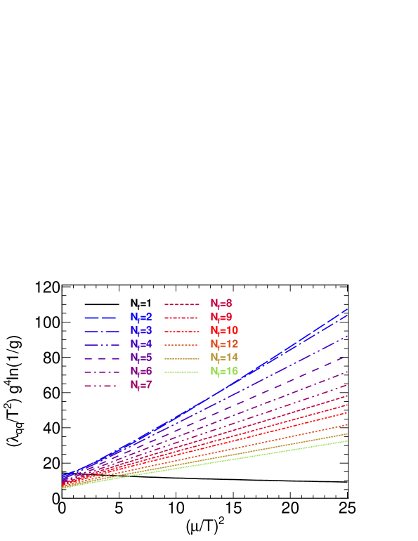
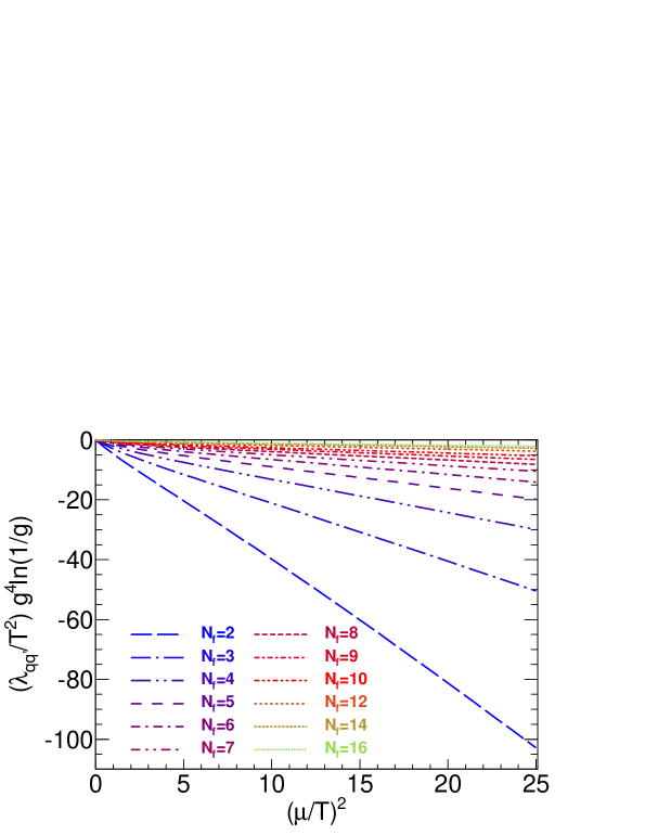
Figure 1: (color online). The normalized diagonal conductivity $\tilde{\lambda}_{qq}$ (upper panel) and off-diagonal conductivity $\tilde{\lambda}_{qq^{\prime}}$ (lower panel) as functions of $(\mu/T)^{2}$ for different $N_{f}$.

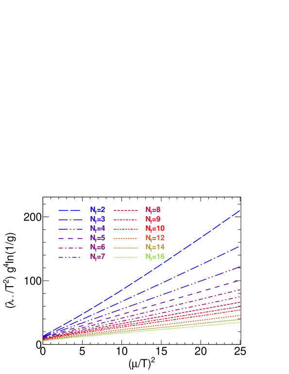
Figure 2: (color online). The normalized conductivities $\tilde{\lambda}_{+}$ (upper panel) and $\tilde{\lambda}_{-}$ (lower panel) as functions of $(\mu/T)^{2}$ for different $N_{f}$ .

$\tilde{\lambda}_{qq}$ and $\tilde{\lambda}_{qq^{\prime}}$ are shown as functions of $(\mu/T)^{2}$ in Fig. 1 for various $N_{f}$ with $N_{f}\leq 16$ such that the system is asymptotically free, while $\tilde{\lambda}_{+}$ and $\tilde{\lambda}_{-}$ are shown in Fig. 2 (note that there is no $\tilde{\lambda}_{qq^{\prime}}$ or $\tilde{\lambda}_{-}$ for $N_{f}=1$). The fact that the matrix $\lambda$ is positive definite makes $\tilde{\lambda}_{qq}$, $\tilde{\lambda}_{+}$ and $\tilde{\lambda}_{-}$ positive, but it imposes no constraint on the sign of $\tilde{\lambda}_{qq^{\prime}}$.

When $(\mu/T)^{2}\rightarrow 0$, we can expand $\tilde{\lambda}_{qq}=a_{0}+a_{1}(\mu/T)^{2}+...$, and $\tilde{\lambda}_{qq^{\prime}}=a_{0}^{\prime}+a_{1}^{\prime}(\mu/T)^{2}+...$. We find $a_{0}^{\prime}=0$ for all $N_{f}$ while the values of $a_{0},a_{1}$ and $a_{1}^{\prime}$ for different $N_{f}$ are tabulated in Table. 1. Our result for $a_{0}$ agrees within $0.1\%$ to that of Arnold, Moore and Yaffe (AMY) calculated up to $N_{f}=6$ listed in Table III of Ref. Arnold:2000dr .

The $a_{0}^{\prime}=0$ property is due to a bigger symmetry enjoyed by the LL results: if we just change all the quarks of flavor $a$ into anti-quarks while the rest of the system stays the same, then as far as collision is concerned, the other quarks and the gluons will not feel any difference. This is because the LL result only depends on two-particle scattering, and although this action could change the sign of certain amplitudes, it does not change the collision rate. For example, the amplitudes of $q_{a}q_{b}\rightarrow$ $q_{a}q_{b}$ and $\bar{q}_{a}q_{b}\rightarrow$ $\bar{q}_{a}q_{b}$ ($a\neq b$) have different signs because one of the couplings changes sign when we change the color into its anti-color, but the amplitude squared is of the same. This makes the diagonal terms even in all the chemical potentials

$$\lambda_{aa}\left(\pm\mu_{1},\pm\mu_{2},\cdots,\pm\mu_{N_{f}}\right)=\lambda_{aa}\left(\mu_{1},\mu_{2},\cdots,\mu_{N_{f}}\right),$$ (54)

while the off-diagonal term $\lambda_{ab}$ is odd in $\mu_{a}$ and $\mu_{b}$ but even in other chemical potentials

$$\lambda_{ab}\left(\pm\mu_{1},\cdots,\pm\mu_{a},\cdots,\pm\mu_{b},\cdots,\pm\mu_{N_{f}}\right)$$

$$=\text{sign}\left(\mu_{a}\mu_{b}\right)\lambda_{ab}\left(\mu_{1},\cdots,\mp\mu_{a},\cdots,\mp\mu_{b},\cdots,\mu_{N_{f}}\right).$$ (55)

Thus, at the LL order, $\lambda$ becomes diagonal when all the chemical potentials vanish.

To understand the other features of $\tilde{\lambda}_{qq}$ and $\tilde{\lambda}_{qq^{\prime}}$, we first turn to $\tilde{\lambda}_{+}$ and $\tilde{\lambda}_{-}$ in the $(T/\mu)^{2}\rightarrow 0$ limit. In this large chemical potential limit, the quark contribution dominates over those of anti-quark and gluon. The Fermi-Dirac distribution function $f^{q_{a}}$ of quark $q_{a}$ multiplied by its Pauli blocking factor $F^{q_{a}}$ can be well approximated by a $\delta-$function, $f^{q_{a}}F^{q_{a}}\simeq T\delta(E_{p}-\mu)$.

We then first set $\bm{\nabla}(\beta\mu_{a})=\bm{\nabla}(\beta\mu)$ for all $a$ so all the currents $\bm{\nu}_{a}$ becomes identical. $\lambda_{+}$ can be rewritten as $\sum_{a,b}\lambda_{ab}$, and Eq. (42) yields

$$\lambda_{+}\simeq-\frac{\beta}{3}N_{q}\int\frac{d^{3}p}{(2\pi)^{3}}T\delta(E_{p}-\mu)\mathbf{p}\cdot\mathbf{A}\sum_{a,b,c=1}^{N_{f}}\left(\frac{n_{b}}{\epsilon+P}-\frac{1}{\mu}\delta_{ca}\right).$$ (56)

The summation gives $N_{f}^{2}\left(\frac{n\mu}{\epsilon+P}-1\right)\propto N_{f}^{2}Ts/(\epsilon+P)\propto N_{f}^{2}T^{2}/\mu^{2}$ and $\lambda_{+}\propto N_{f}^{2}T^{2}A$. On the other hand, Eq.(44) gives $\lambda_{+}\propto N_{f}^{4}\mu^{2}A^{2}$ where $N_{f}^{4}$ comes from summing the $a$, $b$, $c$, $d$ indices of $D_{q_{c}q_{d}\rightarrow q_{c}q_{d}}^{ab}$ and we have used $f_{k_{1}}^{c_{1}}f_{k_{2}}^{c_{2}}F_{k_{3}}^{c_{3}}F_{k_{4}}^{c_{4}}\propto T^{2}$ in Eq.(45). These two conditions yield $\lambda_{+}\propto N_{f}^{0}T^{4}/\mu^{2}$. This is indeed what happens in Fig. 2 at large $\mu$ (although the $1/\mu^{2}$ dependence is not so obvious in this plot but we have checked this at much larger $\mu^{2}/T^{2}$).

We can perform the similar counting to the scaling of $\lambda_{-}$. From Eq. (42), $\lambda_{-}\propto N_{f}\mu^{2}A$ and from Eq.(44) $\lambda_{-}\propto N_{f}^{3}\mu^{2}A^{2}$. Thus, $\lambda_{-}\propto\mu^{2}/N_{f}$ which is also observed in Fig. 2. The main difference in $\lambda_{+}/N_{f}$ and $\lambda_{-}$ is the $T/\mu$ dependence—$\lambda_{-}$ has no cancellation factor of $\left(\frac{n\mu}{\epsilon+P}-1\right)\propto T^{2}$ in large $\mu$.

The different $\mu$ scaling between $\lambda_{+}$ and $\lambda_{-}$ at large $\mu$ is due to collisions, which change the direction of the current and reduce the conductivity. While both flavor singlet and non-singlet fermions can collide among themselves, they do not collide with each other (the scattering amplitude vanishes). Thus, when $\mu$, the flavor singlet chemical potential, is increased, the flavor singlet current experiences more collisions. Therefore the flavor singlet conductivity $\lambda_{+}$ is reduced. For the flavor non-singlet current, the increase of $\mu$ does not affect the collision. However, it will increase the averaged fermi momentum such that the induced current and the flavor non-singlet conductivity $\lambda_{-}$ will be increased.

Given the large $\mu$ behavior of $\tilde{\lambda}_{+}$ and $\tilde{\lambda}_{-}$, the large $\mu$ behavior of $\tilde{\lambda}_{qq}$ and $\tilde{\lambda}_{qq^{\prime}}$ is now easily reconstructed: $\tilde{\lambda}_{qq}\simeq(N_{f}-1)\tilde{\lambda}_{-}/N_{f}\propto(N_{f}-1)\mu^{2}/T^{2}N_{f}^{2}$ ($N_{f}\geq 2$) and $\tilde{\lambda}_{qq^{\prime}}\simeq-\tilde{\lambda}_{-}/N_{f}\propto-\mu^{2}/T^{2}N_{f}^{2}$. The sign of $\tilde{\lambda}_{qq^{\prime}}$ can be best understood from the flavor non-singlet current effect such that a gradient of $\mu_{a}$ induces anti-$b$ currents ($b\neq a$) and yields $\tilde{\lambda}_{qq^{\prime}}<0$. We can then interpolate $\tilde{\lambda}_{qq^{\prime}}$ to $\tilde{\lambda}_{qq^{\prime}}=0$ at zero $\mu$. There is no non-trivial structure at intermediate $\mu$. For $\tilde{\lambda}_{qq}$, the $N_{f}=1$ curve seems to be at odd with other $N_{f}$ curves, but this anomaly disappears when viewed in the $\tilde{\lambda}_{+}$ plot.

The fact that $\lambda_{qq}>0$ while $\lambda_{qq^{\prime}}<0$ at finite $\mu$ is intriguing. It means a gradient $\bm{\nabla}\mu_{a}$ can drive a current $\bm{\nu}_{a}$ along the $-\bm{\nabla}\mu_{a}$ direction, but it will also drive currents of different flavors in the opposite direction. This backward current phenomenon seems counter intuitive at the first sight. But the physics behind is just that the flavor singlet current experiences more collisions in a flavor singlet medium than the flavor non-singlet ones. If the medium is flavor non-singlet, e.g. $\mu_{1}=-\mu_{2}\neq 0$ while the other chemical potentials all vanish, then the flavor non-singlet current $\bm{\nu}_{2}-\bm{\nu}_{1}$ will experience more collisions than the flavor singlet current. Therefore, we will have $\lambda_{12}>0$. This is consistent with Eq.(55) derived from the symmetry of the LL order along. Thus the simple explanation based on collisions that we presented above seems quite generic. It might happen in other systems such as cold atoms as well. In that case, cold atom experiments might be the most promising ones to observe this backward current phenomenon.

Table 1: The coefficients in the $(\mu/T)^{2}$ expansions of $\tilde{\lambda}_{qq}$ and $\tilde{\lambda}_{qq^{\prime}}$ for small $\mu/T$. Our result for $\mu/T=0$ agrees within $0.1\%$ to that of Arnold, Moore and Yaffe calculated up to $N_{f}=6$ Arnold:2000dr .

$N_{f}$ $a_{0}$ $a_{1}$ $a_{1}^{\prime}$ $N_{f}$ $a_{0}$ $a_{1}$ $a_{1}^{\prime}$ 1 14.3676 -0.3077 - 9 7.8019 2.1076 -0.7572 2 12.9989 1.7347 -5.0372 10 7.3806 1.9880 -0.6404 3 11.8688 2.3969 -3.3569 11 7.0025 1.8766 -0.5487 4 10.9197 2.5757 -2.3922 12 6.6612 1.7731 -0.4754 5 10.1113 2.5680 -1.7906 13 6.3517 1.6791 -0.4159 6 9.4145 2.4791 -1.3909 14 6.0697 1.5917 -0.3668 7 8.8076 2.3600 -1.1117 15 5.8117 1.5121 -0.3260 8 8.2743 2.2319 -0.9090 16 5.5747 1.4384 -0.2916

V Summary

We have calculated the conductivity matrix of a weakly coupled quark-gluon plasma at the leading-log order. By setting all quark chemical potentials to be identical, the diagonal conductivities become degenerate and positive, while the off-diagonal ones become degenerate but negative (or zero when the chemical potential vanishes). This means a potential gradient of a certain fermion flavor can drive backward currents of other flavors. A simple explanation is provided for this seemingly counter intuitive phenomenon. It is speculated that this phenomenon is generic and most easily measured in cold atom experiments.

Acknowledgement: SP thanks Tomoi Koide and Xu-guang Huang for helpful discussions on the Onsager relation. JWC thanks Jan M. Pawlowski for useful discussions and the U. of Heidelberg for hospitality. JWC, YFL and SP are supported by the CTS and CASTS of NTU and the NSC (102-2112-M-002-013-MY3) of ROC. YKS is supported in part by the CCNU-QLPL Innovation Fund under grant No. QLPL2011P01. This work is also supported by the National Natural Science Foundation of China under grant No. 11125524 and 11205150, and in part by the China Postdoctoral Science Foundation under the grant No. 2011M501046.

References

- (1) I. Arsene et al. [BRAHMS Collaboration], Nucl. Phys. A 757, 1 (2005) [nucl-ex/0410020].
- (2) K. Adcox et al. [PHENIX Collaboration], Nucl. Phys. A 757, 184 (2005) [nucl-ex/0410003].
- (3) B. B. Back, M. D. Baker, M. Ballintijn, D. S. Barton, B. Becker, R. R. Betts, A. A. Bickley and R. Bindel et al., Nucl. Phys. A 757, 28 (2005) [nucl-ex/0410022].
- (4) J. Adams et al. [STAR Collaboration], Nucl. Phys. A 757, 102 (2005) [nucl-ex/0501009].
- (5) H. Song, S. A. Bass, U. Heinz, T. Hirano and C. Shen, Phys. Rev. Lett. 106, 192301 (2011) [Erratum-ibid. 109, 139904 (2012)].
- (6) P. Kovtun, D. T. Son and A. O. Starinets, Phys. Rev. Lett. 94, 111601 (2005).
- (7) J. M. Maldacena, Adv. Theor. Math. Phys. 2, 231 (1998) [Int. J. Theor. Phys. 38, 1113 (1999)].
- (8) S. S. Gubser, I. R. Klebanov and A. M. Polyakov, Phys. Lett. B 428, 105 (1998)
- (9) E. Witten, Adv. Theor. Math. Phys. 2, 253 (1998)
- (10) P. B. Arnold, G. D. Moore and L. G. Yaffe, JHEP 0011, 001 (2000) [hep-ph/0010177].
- (11) P. B. Arnold, G. D. Moore and L. G. Yaffe, JHEP 0305, 051 (2003) [hep-ph/0302165].
- (12) J.-W. Chen, J. Deng, H. Dong and Q. Wang, Phys. Rev. D 83, 034031 (2011) [Erratum-ibid. D 84, 039902 (2011)] [arXiv:1011.4123 [hep-ph]].
- (13) J. -W. Chen, J. Deng, H. Dong and Q. Wang, Phys. Rev. C 87, 024910 (2013) [arXiv:1107.0522 [hep-ph]].
- (14) L. P. Csernai, J. I. Kapusta and L. D. McLerran, Phys. Rev. Lett. 97, 152303 (2006).
- (15) J.-W. Chen and E. Nakano, Phys. Lett. B 647, 371 (2007) [hep-ph/0604138].
- (16) J.-W. Chen, Y. -F. Liu, Y.-K. Song and Q. Wang, Phys. Rev. D 87, 036002 (2013) [arXiv:1212.5308 [hep-ph]].
- (17) J.-W. Chen, Y. -H. Li, Y. -F. Liu and E. Nakano, Phys. Rev. D 76, 114011 (2007) [hep-ph/0703230].
- (18) D. Kharzeev, K. Tuchin, JHEP 0809, 093 (2008).
- (19) F. Karsch, D. Kharzeev, K. Tuchin, Phys. Lett. B663, 217-221
- (20) H. B. Meyer, JHEP 1004, 099 (2010).
- (21) P. B. Arnold, C. Dogan and G. D. Moore, Phys. Rev. D 74, 085021 (2006) [hep-ph/0608012].
- (22) J.-W. Chen and J. Wang, Phys. Rev. C 79, 044913 (2009) [arXiv:0711.4824 [hep-ph]].
- (23) D. Fernandez-Fraile and A. Gomez Nicola, Phys. Rev. Lett. 102, 121601 (2009).
- (24) E. Lu, G. D. Moore, Phys. Rev. C83, 044901 (2011).
- (25) A. Dobado, F. J. Llanes-Estrada and J. M. Torres-Rincon, Phys. Lett. B 702, 43 (2011).
- (26) P. Chakraborty and J. I. Kapusta, Phys. Rev. C 83, 014906 (2011).
- (27) H. Dong, N. Su and Q. Wang, Phys. Rev. D 75, 074016 (2007) [astro-ph/0702104].
- (28) M. G. Alford and A. Schmitt, J. Phys. G 34, 67 (2007) [nucl-th/0608019].
- (29) M. G. Alford, M. Braby and A. Schmitt, J. Phys. G 35, 115007 (2008) [arXiv:0806.0285 [nucl-th]].
- (30) B. A. Sa’d, I. A. Shovkovy and D. H. Rischke, Phys. Rev. D 75, 065016 (2007) [astro-ph/0607643].
- (31) B. A. Sa’d, I. A. Shovkovy and D. H. Rischke, Phys. Rev. D 75, 125004 (2007) [astro-ph/0703016].
- (32) X. Wang and I. A. Shovkovy, Phys. Rev. D 82, 085007 (2010) [arXiv:1006.1293 [hep-ph]].
- (33) X. -G. Huang and J. Liao, Phys. Rev. Lett. 110, 232302 (2013) [arXiv:1303.7192 [nucl-th]].
- (34) L. McLerran and V. Skokov, arXiv:1305.0774 [hep-ph].
- (35) H. -T. Ding, A. Francis, O. Kaczmarek, F. Karsch, E. Laermann and W. Soeldner, Phys. Rev. D 83, 034504 (2011) [arXiv:1012.4963 [hep-lat]].
- (36) A. Amato, G. Aarts, C. Allton, P. Giudice, S. Hands and J. -I. Skullerud, arXiv:1307.6763 [hep-lat].
- (37) S. -x. Qin, arXiv:1307.4587 [nucl-th].
- (38) W. Israel and J. M. Stewart, Annals Phys. 118, 341 (1979).
- (39) S. Pu, arXiv:1108.5828 [hep-ph].
- (40) S. Jeon, Phys. Rev. D 52, 3591 (1995).
- (41) Y. Hidaka and T. Kunihiro, Phys. Rev. D 83, 076004 (2011).
- (42) J. S. Gagnon and S. Jeon, Phys. Rev. D 76, 105019 (2007).
- (43) P. B. Arnold, G. D. Moore and L. G. Yaffe, JHEP 0301, 030 (2003) [hep-ph/0209353].
- (44) S. Mrowczynski and M. H. Thoma, Phys. Rev. D 62, 036011 (2000) [hep-ph/0001164].