Completeness Results for Parameterized Space Classes

Abstract

The parameterized complexity of a problem is generally considered “settled” once it has been shown to lie in FPT or to be complete for a class in the W-hierarchy or a similar parameterized hierarchy. Several natural parameterized problems have, however, resisted such a classification. At least in some cases, the reason is that upper and lower bounds for their parameterized space complexity have recently been obtained that rule out completeness results for parameterized time classes. In this paper, we make progress in this direction by proving that the associative generability problem and the longest common subsequence problem are complete for parameterized space classes. These classes are defined in terms of different forms of bounded nondeterminism and in terms of simultaneous time–space bounds. As a technical tool we introduce a “union operation” that translates between problems complete for classical complexity classes and for W-classes.

1 Introduction

Parameterization has become a powerful paradigm in complexity theory, both in theory and practice. Instead of just considering the runtime of an algorithm as a function of the input length, we analyse the runtime as a multivariate function depending on a number of different problem parameters, the input length being just one of them. While in classical complexity theory instead of “runtime” many other resource bounds have been studied in great detail, in the parameterized world the focus has lain almost entirely on time complexity. This changed when in a number of papers [5, 8, 12] it was shown for different natural problems, including the vertex cover problem, the feedback vertex set problem, and the longest common subsequence problem, that their parameterized space complexity is of interest. Indeed, the parameterized space complexity of natural problems can explain why some problems in $\mathrm{FPT}$ are easier to solve than others (namely, because they lie in much smaller space classes) and why some problems cannot be classified as complete for levels of the weft hierarchy (namely, because upper and lower bounds on their space complexity rule out such completeness results unless unlikely collapses occur).

Our Contributions.

In the present paper, we present completeness results of natural parameterized problems for different parameterized space complexity classes. The classes we study are of two kinds: First, parameterized classes of bounded nondeterminism and, second, parameterized classes where the space and time resources of the machines are bounded simultaneously. In both cases, we introduce the classes for systematic reasons, but also because they are needed to classify the complexity of the natural problems that we are interested in.

In the context of bounded nondeterminism, we introduce a general “union operation” that turns any language into a parameterized problem in such a way that completeness of the language for some complexity class $C$ carries over to completeness of the parameterized problem for a class “$\mathchoice{\text{\small$\mathrm{paraW}$}}{\text{\small$\mathrm{paraW}$}}{\text{$\mathrm{paraW}$}}{\text{$\mathrm{paraW}$}}C$,” which we will define rigorously later. Building on this result, we show that many union versions of graph problems are complete for $\mathrm{paraW}$$\mathrm{NL}$ and $\mathrm{paraW}$$\mathrm{L}$, but the theorem can also be used to show that $p\text{-}\penalty 15{\text{{weighted-sat}}}$ is complete for $\mathchoice{\text{\small$\mathrm{paraW}$}}{\text{\small$\mathrm{paraW}$}}{\text{$\mathrm{paraW}$}}{\text{$\mathrm{paraW}$}}\mathchoice{\text{\small$\mathrm{NC}$}}{\text{\small$\mathrm{NC}$}}{\text{$\mathrm{NC}$}}{\text{$\mathrm{NC}$}}^{1}$. Our technically most challenging result is that the associative generability problem parameterized by the generator set size is complete for the class $\mathrm{paraWN}$$\mathrm{L}$.

Regarding time–space classes, we present different problems that are complete for the class of problems solvable “nondeterministically in fixed-parameter time and slice-wise logarithmic space.” Among these problems are the longest common subsequence problem parameterized by the number of strings, but also the acceptance problem for certain cellular automata parameterized by the number of cells and also a simple but useful pebble game.

Related Work.

Early work on parameterized space classes is due to Cai et al. [5] who introduced the classes $\mathrm{para\text{-}}$$\mathrm{L}$ and $\mathrm{para\text{-}}$$\mathrm{NL}$, albeit under different names, and showed that several important problems in $\mathrm{FPT}$ lie in these classes: the parameterized vertex cover problem lies in $\mathrm{para\text{-}}$$\mathrm{L}$ and the parameterized $k$-leaf spanning tree problem lies in $\mathrm{para\text{-}}$$\mathrm{NL}$. Later, Flum and Grohe [10] showed that the parameterized model checking problem of first-order formulas on graphs of bounded degree lies in $\mathrm{para\text{-}}$$\mathrm{L}$. In particular, standard parameterized graph problems belong to $\mathrm{para\text{-}}$$\mathrm{L}$ when we restrict attention to bounded-degree graphs. Recently, Guillemot [12] showed that the longest common subsequence problem (lcs) is equivalent under fpt-reductions to the short halting problem for ntms, where the time and space bounds are part of the input and the space bound is the parameter. Our results differ from Guillemot’s insofar as we use weaker reductions (para-$\mathrm{L}$- rather than fpt-reductions) and prove completeness for a class defined using a machine model rather than for a class defined as a reduction closure. The paper [8] by Elberfeld and us is similar to the present paper insofar as it also introduces new parameterized space complexity classes and presents upper and lower bounds for natural parameterized problems. The core difference is that in the present paper we focus on completeness results for natural problems rather than “just” on upper and lower bounds.

Organisation of This Paper.

In Section 2 we review the parameterized space classes previously studied in the literature and introduce some new classes that will be needed in the later sections. For some of the classes from the literature we propose new names in order to systematise the naming and to make connections between the different classes easier to spot. In Section 3 we study problems complete for classes defined in terms of bounded nondeterminism, in Section 4 we do the same for time–space classes.

Due to lack of space, all proofs have been omitted. They can be found in the technical report version of this paper.

2 Parameterized Space Classes

Before we turn our attention to parameterized space classes, let us first review some basic terminology. As in [8], we define a parameterized problem as a pair $(Q,\kappa)$ of a language $Q\subseteq\Sigma^{*}$ and a parameterization $\kappa\colon\Sigma^{*}\to\mathbb{N}$ that maps input instances to parameter values and that is computable in logarithmic space. For a classical complexity class $C$, a parameterized problem $(Q,\kappa)$ belongs to the para-class $\mathchoice{\text{\small$\mathrm{para\text{-}}$}}{\text{\small$\mathrm{para\text{-}}$}}{\text{$\mathrm{para\text{-}}$}}{\text{$\mathrm{para\text{-}}$}}C$ if there are an alphabet $\Pi$, a computable function $\pi\colon\mathbb{N}\to\Pi^{*}$, and a language $A\subseteq\Sigma^{*}\times\Pi^{*}$ with $A\in C$ such that for all $x\in\Sigma^{*}$ we have $x\in Q\iff\big{(}x,\pi\big{(}\kappa(x)\big{)}\big{)}\in A$. The problem is in the X-class $\mathchoice{\text{\small$\mathrm{X}$}}{\text{\small$\mathrm{X}$}}{\text{$\mathrm{X}$}}{\text{$\mathrm{X}$}}C$ if for every number $w\in\mathbb{N}$ the slice $Q_{w}=\{\,x\mid\text{$x\in Q$ and $\kappa(x)=w$}\}$ lies in $C$. It is immediate from the definition that $\mathchoice{\text{\small$\mathrm{para\text{-}}$}}{\text{\small$\mathrm{para\text{-}}$}}{\text{$\mathrm{para\text{-}}$}}{\text{$\mathrm{para\text{-}}$}}C\subseteq\mathchoice{\text{\small$\mathrm{X}$}}{\text{\small$\mathrm{X}$}}{\text{$\mathrm{X}$}}{\text{$\mathrm{X}$}}C$ holds.

The “popular” class $\mathrm{FPT}$ is the same as $\mathrm{para\text{-}}$$\mathrm{P}$. In terms of the $O$-notation, a parameterized problem $(Q,\kappa)$ is in $\mathrm{para\text{-}}$$\mathrm{P}$ if there is a function $f\colon\mathbb{N}\to\mathbb{N}$ such that the question $x\in Q$ can be decided within time $f(\kappa(x))\cdot|x|^{O(1)}$. By comparison, $(Q,\kappa)$ is in $\mathrm{para\text{-}}$$\mathrm{L}$ if $x\in Q$ can be decided within space $f(\kappa(x))+O(\log|x|)$; and for $\mathrm{para\text{-}}$$\mathrm{PSPACE}$ the space requirement is $f(\kappa(x))\cdot|x|^{O(1)}$. The class $\mathrm{XP}$ is in wide use in parameterized complexity theory; the logarithmic space classes $\mathrm{XL}$ and $\mathrm{XNL}$ have previously been studied by Chen et al. [10, 6].

To simplify the notation, let us write $f_{x}$ for $f\big{(}\kappa(x)\big{)}$ and $n$ for $|x|$ in the following. Then the time bound for $\mathrm{para\text{-}}$$\mathrm{P}$ can be written as $f_{x}n^{O(1)}$ and the space bound for $\mathrm{para\text{-}}$$\mathrm{L}$ as $f_{x}+O(\log n)$.

Parameterized logspace reductions ($\mathrm{para\text{-}}$$\mathrm{L}$-reductions) are the natural restriction of fpt-reductions to logarithmic space: A $\mathrm{para\text{-}}$$\mathrm{L}$-reduction from a parameterized problem $(Q_{1},\kappa_{1})$ to $(Q_{2},\kappa_{2})$ is a mapping $r\colon\Sigma_{1}^{*}\to\Sigma_{2}^{*}$ such that

1. for all $x\in\Sigma_{1}^{*}$ we have $x\in Q_{1}\iff r(x)\in Q_{2}$,

2. $\kappa_{2}\big{(}r(x)\big{)}\leq g\big{(}\kappa_{1}(x)\big{)}$ for some computable function $g$, and,

3. $r$ is $\mathrm{para\text{-}}$$\mathrm{L}$-computable with respect to $\kappa_{1}$ (that is, there is a Turing machine that outputs $r(x)$ on input $x$ and needs space at most $f(\kappa_{1}(x))+O(\log|x|)$ for some computable function $f$).

Using standard arguments one can show that all classes in this paper are closed with respect to $\mathrm{para\text{-}}$$\mathrm{L}$-reductions; with the possible exception of $\mathchoice{\text{\small$\mathrm{paraW}$}}{\text{\small$\mathrm{paraW}$}}{\text{$\mathrm{paraW}$}}{\text{$\mathrm{paraW}$}}\mathchoice{\text{\small$\mathrm{NC}$}}{\text{\small$\mathrm{NC}$}}{\text{$\mathrm{NC}$}}{\text{$\mathrm{NC}$}}^{1}$, a class we encounter in Theorem 3.2. Throughout this paper, all completeness and hardness results are meant with respect to $\mathrm{para\text{-}}$$\mathrm{L}$-reductions.

2.1 Parameterized Bounded Nondeterminism

While the interplay of nondeterminism and parameterized space may seem to be simple at first sight ($\mathrm{NL}$ is closed under complement and $\mathrm{NPSPACE}$ is even equal to $\mathrm{PSPACE}$, so only $\mathrm{XNL}$ and $\mathrm{para\text{-}}$$\mathrm{NL}$ appear interesting), a closer look reveals that useful and interesting new classes arise when we bound the amount of nondeterminism used by machines in dependence on the parameter. For this, it is useful to view nondeterministic computations as deterministic computations using “choice tapes” or “tapes filled with nondeterministic bits.” These are extra tapes for a deterministic Turing machine, and an input word is accepted if there is at least one bitstring that we can place on this extra tape at the beginning of the computation such that the Turing machine accepts. It is well known that $\mathrm{NP}$ and $\mathrm{NL}$ can be defined in this way using deterministic polynomial-time or logarithmic-space machines, respectively, that have one-way access to a choice tape. (For $\mathrm{NP}$ it makes no difference whether we have one- or two-way access, but logspace dtms with access to a two-way choice tape can accept all of $\mathrm{NP}$.)

Classes of bounded nondeterminism arise when we restrict the length of the bitstrings on the choice tape. For instance, the classes $\beta^{h}$ for $h\geq 1$, see [16] and also [1] for variants, are defined in the same way as $\mathrm{NP}$ above, only the length of the bitstring on the choice tape may be at most $O(\log^{h}n)$. Classes of parameterized bounded nondeterminism arise when we restrict the length the bitstring on the choice tape in dependence not only on the input length, but also of the parameter. Furthermore, in the context of bounded space computations, it also makes a difference whether we have one-way or two-way access to the choice tapes.

Definition 2.1.

Let $C$ be a complexity class defined in terms of a deterministic Turing machine model (like $\mathrm{L}$ or $\mathrm{P}$). We define $\mathchoice{\text{\small$\mathrm{para\exists^{\leftrightarrow}}$}}{\text{\small$\mathrm{para\exists^{\leftrightarrow}}$}}{\text{$\mathrm{para\exists^{\leftrightarrow}}$}}{\text{$\mathrm{para\exists^{\leftrightarrow}}$}}C$ as the class of parameterized problems $(Q,\kappa)$ for which there exists a $C$-machine $M$, an alphabet $\Pi$, and a computable function $\pi\colon\mathbb{N}\to\Pi^{*}$ such that: For every $x\in\Sigma^{*}$ we have $x\in Q$ if, and only if, there exists a bitstring $b\in\{0,1\}^{*}$ such that $M$ accepts with $(x,\pi(\kappa(x)))$ on its input tape and $b$ on the two-way choice tape. We define $\mathchoice{\text{\small$\mathrm{para\exists^{\to}}$}}{\text{\small$\mathrm{para\exists^{\to}}$}}{\text{$\mathrm{para\exists^{\to}}$}}{\text{$\mathrm{para\exists^{\to}}$}}C$ similarly, only access to the choice tape is now one-way.

We define $\mathchoice{\text{\small$\mathrm{para\exists^{\leftrightarrow}_{\mathit{f}\!\log}}$}}{\text{\small$\mathrm{para\exists^{\leftrightarrow}_{\mathit{f}\!\log}}$}}{\text{$\mathrm{para\exists^{\leftrightarrow}_{\mathit{f}\!\log}}$}}{\text{$\mathrm{para\exists^{\leftrightarrow}_{\mathit{f}\!\log}}$}}C$ and $\mathchoice{\text{\small$\mathrm{para\exists^{\to}_{\mathit{f}\!\log}}$}}{\text{\small$\mathrm{para\exists^{\to}_{\mathit{f}\!\log}}$}}{\text{$\mathrm{para\exists^{\to}_{\mathit{f}\!\log}}$}}{\text{$\mathrm{para\exists^{\to}_{\mathit{f}\!\log}}$}}C$ in the same way, but the length of $b$ may be at most $|\pi(\kappa(x))|\cdot O(\log n)$.

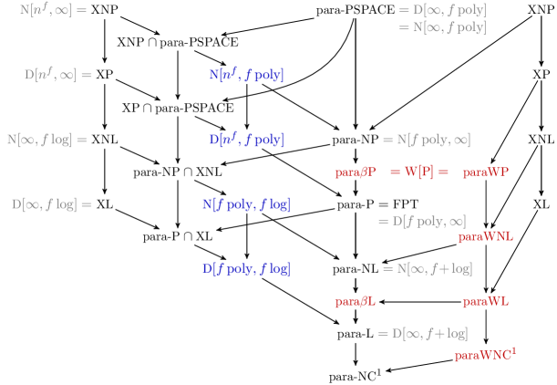
Figure 1: In this inclusion diagram bounded nondeterminism classes are shown in red and time–space classes in blue. The X-classes are shown twice to keep the diagram readable. All known inclusions are indicated, where $C\to D$ means $C\supseteq D$.

Observe that, as argued earlier, $\mathchoice{\text{\small$\mathrm{para\exists^{\leftrightarrow}}$}}{\text{\small$\mathrm{para\exists^{\leftrightarrow}}$}}{\text{$\mathrm{para\exists^{\leftrightarrow}}$}}{\text{$\mathrm{para\exists^{\leftrightarrow}}$}}\mathchoice{\text{\small$\mathrm{L}$}}{\text{\small$\mathrm{L}$}}{\text{$\mathrm{L}$}}{\text{$\mathrm{L}$}}=\mathchoice{\text{\small$\mathrm{para\exists^{\leftrightarrow}}$}}{\text{\small$\mathrm{para\exists^{\leftrightarrow}}$}}{\text{$\mathrm{para\exists^{\leftrightarrow}}$}}{\text{$\mathrm{para\exists^{\leftrightarrow}}$}}\mathchoice{\text{\small$\mathrm{P}$}}{\text{\small$\mathrm{P}$}}{\text{$\mathrm{P}$}}{\text{$\mathrm{P}$}}=\mathchoice{\text{\small$\mathrm{para\exists^{\to}}$}}{\text{\small$\mathrm{para\exists^{\to}}$}}{\text{$\mathrm{para\exists^{\to}}$}}{\text{$\mathrm{para\exists^{\to}}$}}\mathchoice{\text{\small$\mathrm{P}$}}{\text{\small$\mathrm{P}$}}{\text{$\mathrm{P}$}}{\text{$\mathrm{P}$}}=\mathchoice{\text{\small$\mathrm{para\text{-}}$}}{\text{\small$\mathrm{para\text{-}}$}}{\text{$\mathrm{para\text{-}}$}}{\text{$\mathrm{para\text{-}}$}}\mathchoice{\text{\small$\mathrm{NP}$}}{\text{\small$\mathrm{NP}$}}{\text{$\mathrm{NP}$}}{\text{$\mathrm{NP}$}}$ and $\mathchoice{\text{\small$\mathrm{para\exists^{\to}}$}}{\text{\small$\mathrm{para\exists^{\to}}$}}{\text{$\mathrm{para\exists^{\to}}$}}{\text{$\mathrm{para\exists^{\to}}$}}\mathchoice{\text{\small$\mathrm{L}$}}{\text{\small$\mathrm{L}$}}{\text{$\mathrm{L}$}}{\text{$\mathrm{L}$}}=\mathchoice{\text{\small$\mathrm{para\text{-}}$}}{\text{\small$\mathrm{para\text{-}}$}}{\text{$\mathrm{para\text{-}}$}}{\text{$\mathrm{para\text{-}}$}}\mathchoice{\text{\small$\mathrm{NL}$}}{\text{\small$\mathrm{NL}$}}{\text{$\mathrm{NL}$}}{\text{$\mathrm{NL}$}}$. Also observe that $\mathchoice{\text{\small$\mathrm{para\exists^{\leftrightarrow}_{\mathit{f}log}}$}}{\text{\small$\mathrm{para\exists^{\leftrightarrow}_{\mathit{f}log}}$}}{\text{$\mathrm{para\exists^{\leftrightarrow}_{\mathit{f}log}}$}}{\text{$\mathrm{para\exists^{\leftrightarrow}_{\mathit{f}log}}$}}\mathchoice{\text{\small$\mathrm{P}$}}{\text{\small$\mathrm{P}$}}{\text{$\mathrm{P}$}}{\text{$\mathrm{P}$}}=\mathchoice{\text{\small$\mathrm{para\exists^{\to}_{\mathit{f}log}}$}}{\text{\small$\mathrm{para\exists^{\to}_{\mathit{f}log}}$}}{\text{$\mathrm{para\exists^{\to}_{\mathit{f}log}}$}}{\text{$\mathrm{para\exists^{\to}_{\mathit{f}log}}$}}\mathchoice{\text{\small$\mathrm{P}$}}{\text{\small$\mathrm{P}$}}{\text{$\mathrm{P}$}}{\text{$\mathrm{P}$}}=\mathchoice{\text{\small$\mathrm{W}$}}{\text{\small$\mathrm{W}$}}{\text{$\mathrm{W}$}}{\text{$\mathrm{W}$}}[\mathchoice{\text{\small$\mathrm{P}$}}{\text{\small$\mathrm{P}$}}{\text{$\mathrm{P}$}}{\text{$\mathrm{P}$}}]$ by one of the many possible definitions of $\mathchoice{\text{\small$\mathrm{W}$}}{\text{\small$\mathrm{W}$}}{\text{$\mathrm{W}$}}{\text{$\mathrm{W}$}}[\mathchoice{\text{\small$\mathrm{P}$}}{\text{\small$\mathrm{P}$}}{\text{$\mathrm{P}$}}{\text{$\mathrm{P}$}}]$.

The above definition can easily be extended to the case where a universal quantifier is used instead of an existential one and where sequences of quantifiers are used. This is interpreted in the usual way as having a choice tape for each quantifier and the different “exists … for all”-conditions must be met in the order the quantifiers appear. For instance, for problems in $\mathrm{para\exists^{\leftrightarrow}_{\mathit{f}\!\log}\exists^{\to}}$$\mathrm{L}$ we have $x\in Q$ if, and only if, there exists a bitstring of length $f_{x}\log_{2}n$ for the first, two-way-readable choice tape for which an $\mathrm{NL}$-machine accepts. The classes $\mathchoice{\text{\small$\mathrm{para\text{-}NL}$}}{\text{\small$\mathrm{para\text{-}NL}$}}{\text{$\mathrm{para\text{-}NL}$}}{\text{$\mathrm{para\text{-}NL}$}}[f\log]$, $\mathrm{para\text{-}L\text{-}cert}$, and $\mathrm{para\text{-}NL\text{-}cert}$ introduced in an ad hoc manner by Elberfeld et al. in [8] can now be represented systematically: They are $\mathrm{para\exists^{\to}_{\mathit{f}\!\log}}$$\mathrm{L}$, $\mathrm{para\exists^{\leftrightarrow}_{\mathit{f}\!\log}}$$\mathrm{L}$, and $\mathrm{para\exists^{\leftrightarrow}_{\mathit{f}\!\log}\exists^{\to}}$$\mathrm{L}$, respectively.

In order to make the notation more useful in practice, instead of “$\exists^{\to}$” let us write “$\mathrm{N}$” and instead of “$\exists^{\to}_{\mathit{f}\!\log}$” we write “$\beta$” as is customary. As a new notation, instead of “$\exists^{\leftrightarrow}_{\mathit{f}\!\log}$” and “$\forall^{\leftrightarrow}_{\mathit{f}\!\log}$” we write “$\mathrm{W}$” and “$\mathrm{W_{\forall}}$,” respectively. The three classes of [8] now become $\mathrm{para\beta}$$\mathrm{L}$, $\mathrm{paraW}$$\mathrm{L}$, and $\mathrm{paraWN}$$\mathrm{L}$.

Our reasons for using “W” to denote $\exists^{\leftrightarrow}_{\mathit{f}\!\log}$ will be explained fully in Section 3; for the moment just observe that $\mathchoice{\text{\small$\mathrm{W}$}}{\text{\small$\mathrm{W}$}}{\text{$\mathrm{W}$}}{\text{$\mathrm{W}$}}[\mathchoice{\text{\small$\mathrm{P}$}}{\text{\small$\mathrm{P}$}}{\text{$\mathrm{P}$}}{\text{$\mathrm{P}$}}]=\mathchoice{\text{\small$\mathrm{paraW}$}}{\text{\small$\mathrm{paraW}$}}{\text{$\mathrm{paraW}$}}{\text{$\mathrm{paraW}$}}\mathchoice{\text{\small$\mathrm{P}$}}{\text{\small$\mathrm{P}$}}{\text{$\mathrm{P}$}}{\text{$\mathrm{P}$}}$ holds. To get a better intuition on the W-operator, note that it provides machines with “$f_{x}\log_{2}n$ bits of nondeterministic information” or, equivalently, with “$f_{x}$ many nondeterministic positions in the input” and these bits are provided as part of the input. This allows us to also apply the W-operator to classes like $\mathchoice{\text{\small$\mathrm{NC}$}}{\text{\small$\mathrm{NC}$}}{\text{$\mathrm{NC}$}}{\text{$\mathrm{NC}$}}^{1}$ that are not defined in terms of Turing machines.

The right half of Figure 1 depicts the known inclusions between the introduced classes, the left half shows the classes introduced next.

2.2 Parameterized Time–Space Classes

In classical complexity theory, the major complexity classes are either defined in terms of time complexity ($\mathrm{P}$, $\mathrm{NP}$, $\mathrm{EXP}$) or in terms of space complexity ($\mathrm{L}$, $\mathrm{NL}$, $\mathrm{PSPACE}$), but not both at the same time: by the well-known inclusion chain $\mathchoice{\text{\small$\mathrm{L}$}}{\text{\small$\mathrm{L}$}}{\text{$\mathrm{L}$}}{\text{$\mathrm{L}$}}\subseteq\mathchoice{\text{\small$\mathrm{NL}$}}{\text{\small$\mathrm{NL}$}}{\text{$\mathrm{NL}$}}{\text{$\mathrm{NL}$}}\subseteq\mathchoice{\text{\small$\mathrm{P}$}}{\text{\small$\mathrm{P}$}}{\text{$\mathrm{P}$}}{\text{$\mathrm{P}$}}\subseteq\mathchoice{\text{\small$\mathrm{NP}$}}{\text{\small$\mathrm{NP}$}}{\text{$\mathrm{NP}$}}{\text{$\mathrm{NP}$}}\subseteq\mathchoice{\text{\small$\mathrm{PSPACE}$}}{\text{\small$\mathrm{PSPACE}$}}{\text{$\mathrm{PSPACE}$}}{\text{$\mathrm{PSPACE}$}}=\mathchoice{\text{\small$\mathrm{NPSPACE}$}}{\text{\small$\mathrm{NPSPACE}$}}{\text{$\mathrm{NPSPACE}$}}{\text{$\mathrm{NPSPACE}$}}\subseteq\mathchoice{\text{\small$\mathrm{EXP}$}}{\text{\small$\mathrm{EXP}$}}{\text{$\mathrm{EXP}$}}{\text{$\mathrm{EXP}$}}$ space and time are intertwined in such a way that bounding either automatically bounds the other in a specific way (at least for the major complexity classes). In the parameterized world, interesting new classes arise when we restrict time and space simultaneously: namely whenever the time is “para-restricted” while space is “X-restricted” or vice versa.

Definition 2.2.

For a space bound $s$ and a time bound $t$, both of which may depend on a parameter $k$ and the input length $n$, let $\mathchoice{\text{\small$\mathrm{D}$}}{\text{\small$\mathrm{D}$}}{\text{$\mathrm{D}$}}{\text{$\mathrm{D}$}}[t,s]$ denote the class of all parameterized problems that can be accepted by a deterministic Turing machine in time $t(\kappa(x),|x|)$ and space $s(\kappa(x),|x|)$. Let $\mathchoice{\text{\small$\mathrm{N}$}}{\text{\small$\mathrm{N}$}}{\text{$\mathrm{N}$}}{\text{$\mathrm{N}$}}[t,s]$ denote the corresponding nondeterministic class.

Four cases are of interest: First, $\mathchoice{\text{\small$\mathrm{D}$}}{\text{\small$\mathrm{D}$}}{\text{$\mathrm{D}$}}{\text{$\mathrm{D}$}}[f\mathrm{poly},f\log]$, meaning that $t(k,n)=f(k)\cdot n^{O(1)}$ and $s(k,n)=f(k)\cdot O(\log n)$, contains all problems that are “fixed parameter tractable via a machine needing only slice-wise logarithmic space,” and, second, the nondeterministic counterpart $\mathchoice{\text{\small$\mathrm{N}$}}{\text{\small$\mathrm{N}$}}{\text{$\mathrm{N}$}}{\text{$\mathrm{N}$}}[f\mathrm{poly},f\log]$. The two other cases are $\mathchoice{\text{\small$\mathrm{D}$}}{\text{\small$\mathrm{D}$}}{\text{$\mathrm{D}$}}{\text{$\mathrm{D}$}}[n^{f},f\mathrm{poly}]$ and $\mathchoice{\text{\small$\mathrm{N}$}}{\text{\small$\mathrm{N}$}}{\text{$\mathrm{N}$}}{\text{$\mathrm{N}$}}[n^{f},f\mathrm{poly}]$, which contain problems that are “in slice-wise polynomial time via machines that need only fixed parameter polynomial space.” See Figure 1 for the trivial inclusions between the classes.

In Section 4 we will see that these classes are not only of scholarly interest. Rather, we will show that lcs parameterized by the number of input strings is complete for $\mathchoice{\text{\small$\mathrm{N}$}}{\text{\small$\mathrm{N}$}}{\text{$\mathrm{N}$}}{\text{$\mathrm{N}$}}[f\mathrm{poly},f\log]$.

3 Complete Problems for Bounded Nondeterminism

In this section we present new natural problems that are complete for $\mathrm{paraW}$$\mathrm{NL}$ and $\mathrm{paraW}$$\mathrm{L}$. Previously, it was only known that the following “colored reachability problem” [8] is complete for $\mathrm{paraW}$$\mathrm{NL}$: We are given an edge-colored graph, two vertices $s$ and $t$, and a parameter $k$. The question is whether there is a path from $s$ to $t$ that uses only $k$ colors. Our key tool for proving new completeness results will be the introduction of a “union operation,” which turns $\mathrm{P}$-, $\mathrm{NL}$-, and $\mathrm{L}$-complete problems into $\mathrm{paraW}$$\mathrm{P}$-, $\mathrm{paraW}$$\mathrm{NL}$-, and $\mathrm{paraW}$$\mathrm{L}$-complete problems, respectively. Building on this, we prove the parameterized associative generability problem to be complete for $\mathrm{paraW}$$\mathrm{NL}$. Note that the underlying classical problem is well-known to be $\mathrm{NL}$-complete and, furthermore, if we drop the requirement of associativity, the parameterized and classical versions are known to be complete for $\mathrm{paraW}$$\mathrm{P}$ and $\mathrm{P}$, respectively.

At this point, we remark that Guillemot, in a paper [12] on parameterized time complexity, uses “$\mathrm{WNL}$” to denote a class different from the class $\mathrm{paraW}$$\mathrm{NL}$ defined in this paper. Guillemot chose the name because his definition of the class is derived from one possible definition of $\mathchoice{\text{\small$\mathrm{W}$}}{\text{\small$\mathrm{W}$}}{\text{$\mathrm{W}$}}{\text{$\mathrm{W}$}}[1]$ by replacing a time by a space constraint. Nevertheless, we believe that our definition of a “W-operator” yields the “right analogue” of $\mathchoice{\text{\small$\mathrm{W}$}}{\text{\small$\mathrm{W}$}}{\text{$\mathrm{W}$}}{\text{$\mathrm{W}$}}[\mathchoice{\text{\small$\mathrm{P}$}}{\text{\small$\mathrm{P}$}}{\text{$\mathrm{P}$}}{\text{$\mathrm{P}$}}]$: First, there is the above pattern that parameterized version of problems complete $\mathrm{P}$, $\mathrm{NL}$, and $\mathrm{L}$ tend to be complete for $\mathrm{paraW}$$\mathrm{P}$, $\mathrm{paraW}$$\mathrm{NL}$, and $\mathrm{paraW}$$\mathrm{L}$, respectively. Furthermore, in Section 4 we show that the class $\mathrm{WNL}$ defined and studied by Guillemot is exactly the fpt-reduction closure of the time–space class $\mathchoice{\text{\small$\mathrm{N}$}}{\text{\small$\mathrm{N}$}}{\text{$\mathrm{N}$}}{\text{$\mathrm{N}$}}[f\operatorname{poly},f\log]$.

Union Problems.

For numerous problems studied in complexity theory the input consists of a string in which some positions can be “selected” and the objective is to select a “good” subset of these positions. For instance, for the satisfiability problem we must select some variables such that setting them to true makes a formula true; for the circuit satisfiability problem we must select some input gates such that when they are set to $1$ the circuit evaluates to $1$; and for the exact cover problem we must select some sets from a family of sets so that they form a partition of the union of the family. In the following, we introduce some terminology that allows us to formulate all of these problems in a uniform way and to link them to the W-operator.

Let $\Sigma$ be an alphabet that contains none of the three special symbols $?$, $0$, and $1$. We call a word $t\in(\Sigma\cup\{?\})^{*}$ a template. We call a word $s\in(\Sigma\cup\{0,1\})^{*}$ an instantiation of $t$ if $s$ is obtained from $t$ by replacing exactly the $?$-symbols arbitrarily by $0$- or $1$-symbols. Given instantiations $s_{1},\dots,s_{k}$ of the same template $t$, their union $s$ is the instantiation of $t$ that has a $1$ exactly at those positions $i$ where at least one $s_{j}$ has a $1$ at position $i$ (the union is the “bitwise or” of the instantiated positions and is otherwise equal to the template).

Given a language $A\subseteq(\Sigma\cup\{0,1\})^{*}$, we define three different kinds of union problems for $A$. Each of them is a parameterized problem where the parameter is $k$. As we will see in a moment, the first kind is linked to the W-operator while the last kind links several well-known languages from classical complexity theory to well-known parameterized problems. We will also see that the three kinds of union problems for a language $A$ often all have the same complexity.

1. The input for $p\text{-}\penalty 15{\text{{family-union-}}}A$ are a template $t\in(\Sigma\cup\{?\})^{*}$ and a family $(S_{1},\dots,S_{k})$ of $k$ sets of instantiations of $t$. The question is whether there are $s_{i}\in S_{i}$ for $i\in\{1,\dots,k\}$ such that the union of $s_{1},\dots,s_{k}$ lies in $A$.

2. The input for $p\text{-}\penalty 15{\text{{subset-union-}}}A$ are a template $t\in(\Sigma\cup\{?\})^{*}$, a set $S$ of instantiations of $t$, and a number $k$. The question is whether there exists a subset $R\subseteq S$ of size $|R|=k$ such that the union of $R$’s elements lies in $A$.

3. The input for $p\text{-}\penalty 15{\text{{weighted-union-}}}A$ are a template $t\in(\Sigma\cup\{?\})^{*}$ and a number $k$. The question is whether there exists an instantiation $s$ of $t$ containing exactly $k$ many $1$-symbols such that $s\in A$?

To get an intuition for these definitions, think of instantiations as words written on transparencies with $0$ rendered as an empty box and $1$ as a checked box. Then for the family union problem we are given $k$ heaps of transparencies and the task is to pick one transparency from each heap such that “stacking them on top of each other” yields an element of $A$. For the subset union problem, we are only given one stack and must pick $k$ elements from it. We call the weighted union problem a “union” problem partly in order to avoid a clash with existing terminology and partly because the weighted union problem is the same as the subset union problem for the special set $S$ containing all instantiations of the template of weight $1$.

Concerning the promised link between well-known languages and parameterized problems, consider $A={\text{{circuit-value-problem}}}$ (cvp) where we use $\Sigma$ to encode a circuit and use $0$’s and $1$’s solely to describe an assignment to the input gates. Then the input for $p$-weighted-union-cvp are a circuit with $?$-symbols instead of a concrete assignment together with a number $k$, and the question is whether we can replace exactly $k$ of the $?$-symbols by $1$’s (and the other by $0$’s) so that the resulting instantiation lies in cvp. Clearly, $p\text{-}\penalty 15{\text{{weighted-union-cvp}}}$ is exactly the $\mathchoice{\text{\small$\mathrm{W}$}}{\text{\small$\mathrm{W}$}}{\text{$\mathrm{W}$}}{\text{$\mathrm{W}$}}[\mathchoice{\text{\small$\mathrm{P}$}}{\text{\small$\mathrm{P}$}}{\text{$\mathrm{P}$}}{\text{$\mathrm{P}$}}]$-complete problem $p\text{-}\penalty 15{\text{{circuit-sat}}}$, which asks whether there is a satisfying assignment for a given circuit that sets exactly $k$ input gates to $1$.

Concerning the promised link between the union problems and the W-operator, recall that the operator provides machines with $f_{x}$ nondeterministic indices as part of the input. In particular, a W-machine can mark $f_{x}$ different “parts” of the input – like one element from each of $f_{x}$ many sets in a family, like the elements of a size-$f_{x}$ subset of some set, or like $f_{x}$ many positions in a template. With this observation it is not difficult to see that if $A\in C$, then all union versions of $A$ lie in $\mathchoice{\text{\small$\mathrm{paraW}$}}{\text{\small$\mathrm{paraW}$}}{\text{$\mathrm{paraW}$}}{\text{$\mathrm{paraW}$}}C$. A much deeper observation is that the union versions are also often complete for these classes. In the next theorem, which states this claim precisely, the following definition of a compatible logspace projection $p$ from a language $A$ to a language $B$ is used: First, $p$ must be a logspace reduction from $A$ to $B$. Second, $p$ is a projection, meaning that each symbol of $p(x)$ depends on at most one symbol of $x$. Third, for each word length $n$ there is a single template $t_{n}$ such for all $x\in\Sigma^{n}$ the word $p(x)$ is an instantiation of $t_{n}$.

Theorem 3.1.

Let $C\in\{\mathchoice{\text{\small$\mathrm{NC}$}}{\text{\small$\mathrm{NC}$}}{\text{$\mathrm{NC}$}}{\text{$\mathrm{NC}$}}^{1},\mathchoice{\text{\small$\mathrm{L}$}}{\text{\small$\mathrm{L}$}}{\text{$\mathrm{L}$}}{\text{$\mathrm{L}$}},\mathchoice{\text{\small$\mathrm{NL}$}}{\text{\small$\mathrm{NL}$}}{\text{$\mathrm{NL}$}}{\text{$\mathrm{NL}$}},\mathchoice{\text{\small$\mathrm{P}$}}{\text{\small$\mathrm{P}$}}{\text{$\mathrm{P}$}}{\text{$\mathrm{P}$}}\}$. Let $A$ be complete for $C$ via compatible logspace projections. Then $p\text{-}\penalty 15{\text{{family-union-}}}A$ is complete for $\mathchoice{\text{\small$\mathrm{paraW}$}}{\text{\small$\mathrm{paraW}$}}{\text{$\mathrm{paraW}$}}{\text{$\mathrm{paraW}$}}C$ under para-$\mathrm{L}$-reductions.

Proof.

For containment, on input of a template $t$ and family $(S_{1},\dots,\penalty 0S_{k})$ of sets of instantiations of $t$, a $\mathchoice{\text{\small$\mathrm{paraW}$}}{\text{\small$\mathrm{paraW}$}}{\text{$\mathrm{paraW}$}}{\text{$\mathrm{paraW}$}}C$-machine or -circuit interprets its $k\log_{2}n$ nondeterministic bits as $k$ indices, one for each $S_{i}$. Let $s_{i}\in S_{i}$ be the elements selected in this way. We run a simulation of the $C$-machine (or $C$-circuit) that decides $A$ on the union $s$ of $s_{1},\dots,s_{k}$. For logspace machines, we may not have enough space to write $s$ on a tape, so whenever the machine would like to know the $j$th bit of $u$, we simply compute the bitwise-or of the $j$th positions of the $s_{i}$.

For hardness, consider any problem $(Q,\kappa)\in\mathchoice{\text{\small$\mathrm{paraW}$}}{\text{\small$\mathrm{paraW}$}}{\text{$\mathrm{paraW}$}}{\text{$\mathrm{paraW}$}}C$. By definition, this means the following: There are a language $X\subseteq\Gamma^{*}$ in $C$ and computable functions $\pi\colon\mathbb{N}\to\Pi^{*}$ and $f\colon\mathbb{N}\to\mathbb{N}$ such that $x\in Q$ if, and only if, there is a string $b\in\{0,1\}^{f_{x}\log_{2}n}$ with $(x,\pi(\kappa(x)),b)\in X$. Furthermore, since $A$ is complete for $C$ via compatible logspace projections, we can reduce $X$ to $A$ via some $p$. (As always, $n=|x|$ and $f_{x}=f(\kappa(x))$.)

For the reduction of $(Q,\kappa)$ to $p\text{-}\penalty 15{\text{{family-union-}}}A$, let an input $x$ be given. Our para-$\mathrm{L}$-reduction first computes $\pi(\kappa(x))$. Since our reduction $p$ is compatible, for all possible $b$ the string $p(x,\pi(\kappa(x)),b)$ will have $0$-symbols and $1$-symbols at the same positions and all other positions will not vary with $b$ at all. Our template $t$ will be the string $p(x,\pi(\kappa(x)),b)$ with $?$-symbols placed at these positions (as argued, we can use any $b$).

To define the sets of instances $S_{i}$, observe that the strings $b\in\{0,1\}^{f_{x}\log_{2}n}$ can be thought of as sequences of $f_{x}$ symbols from the alphabet $\Delta=\{0,1\}^{\log_{2}n}$, whose elements we call blocks. For $i\in\{1,\dots,f_{x}\}$ let $S_{i}=\{m_{i}^{\delta}\mid\delta\in\Delta\}$ where $m_{i}^{\delta}$ replaces the $r$th $?$-symbol of the template $t$ by $c\in\{0,1\}$ as follows: If the $r$th position depends on a symbol in $(x,\pi(\kappa(x)),b)$ that lies in a block of $b$, but not in the $i$th block, let $c=0$. Otherwise, let $c$ be whatever symbol ($0$ or $1$) the reduction outputs when the $i$th block is set to $\delta$. This concludes the construction.

As an example for the construction, suppose the reduction $p$ simply doubles its input (so $w$ is mapped to $ww$) and $\pi$ just returns the empty string, and $\Sigma=\{\alpha,\beta,\gamma\}$. Consider, say, $x=\alpha\beta\gamma\alpha$ and assume $f_{x}=2$. We then have $\Delta=\{00,01,10,11\}$. The reduction would produce two sets $S_{1}$ and $S_{2}$. For $S_{1}$, we have a look at what $p$ does on input of a string like $(x,\pi(\kappa(x)),b)$. For simplicity let us ignore parentheses and commas, and consider $b=1111$, so this string would just be $\alpha\beta\gamma\alpha 1111$. The reduction maps this to $\alpha\beta\gamma\alpha 1111\alpha\beta\gamma\alpha 1111$. In this string, the fifth, sixth, thirteenth, and fourteenth bits actually depend on the first block of $\alpha\beta\gamma\alpha 1111$, so the reduction would produce the first set

$$S_{1}=\{ \alpha\beta\gamma\alpha 0000\alpha\beta\gamma\alpha 0000,$$

$$\alpha\beta\gamma\alpha 0100\alpha\beta\gamma\alpha 0100,$$

$$\alpha\beta\gamma\alpha 1000\alpha\beta\gamma\alpha 1000,$$

$$\alpha\beta\gamma\alpha 1100\alpha\beta\gamma\alpha 1100\}.$$

In a similar manner, the reduction would produce the second set

$$S_{2}=\{ \alpha\beta\gamma\alpha 0000\alpha\beta\gamma\alpha 0000,$$

$$\alpha\beta\gamma\alpha 0001\alpha\beta\gamma\alpha 0001,$$

$$\alpha\beta\gamma\alpha 0010\alpha\beta\gamma\alpha 0010,$$

$$\alpha\beta\gamma\alpha 0011\alpha\beta\gamma\alpha 0011\}.$$

Observe that, indeed, we can get every string $p(x,\pi(\kappa(x)),b)$ by taking the union of one string from $S_{1}$ and one string from $S_{2}$.

To see that the reduction is correct, consider the union of the elements of any set $\smash{\{m_{1}^{\delta_{1}}},\dots,\penalty 0m_{f_{x}}^{\delta_{f_{x}}}\}$ where the $m_{i}^{\delta_{i}}$ are chosen from the different $S_{i}$. By construction, their union will be exactly the image of $(x,\pi(\kappa(x)),\delta_{1}\dots\delta_{f_{x}})$ under $p$. In particular, $x\in Q$ holds if, and only if, we can choose one instantiation from each $S_{i}$ such that their union is in $A$. ∎

Parameterized Satisfiability Problems.

Recall that the problem $p$-weighted-union-cvp equals $p$-circuit-sat. Since one can reduce $p$-family-union-cvp to $p$-weighted-union-cvp (via essentially the same reduction as that used in the proof of Theorem 3.2 below), Theorem 3.1 provides us with a direct proof that $p$-circuit-sat${}={}$$p$-weighted-union-cvp is complete for $\mathrm{paraW}$$\mathrm{P}$. We get an even more interesting result when we apply the theorem to bf, the propositional formula evaluation problem. We encode pairs of formulas and assignments in the straightforward way by using $0$ and $1$ solely for the assignment. Since bf is complete for $\mathchoice{\text{\small$\mathrm{NC}$}}{\text{\small$\mathrm{NC}$}}{\text{$\mathrm{NC}$}}{\text{$\mathrm{NC}$}}^{1}$ under compatible logspace reductions, see [3, 2], $p$-family-union-bf is complete for $\mathchoice{\text{\small$\mathrm{paraW}$}}{\text{\small$\mathrm{paraW}$}}{\text{$\mathrm{paraW}$}}{\text{$\mathrm{paraW}$}}\mathchoice{\text{\small$\mathrm{NC}$}}{\text{\small$\mathrm{NC}$}}{\text{$\mathrm{NC}$}}{\text{$\mathrm{NC}$}}^{1}$ by Theorem 3.1. By further reducing the problem to $p$-weighted-union-bf, we obtain:

Theorem 3.2.

$p\text{-}\penalty 15{\text{{weighted-union-bf}}}$ is para-$\mathrm{L}$-complete for $\mathchoice{\text{\small$\mathrm{paraW}$}}{\text{\small$\mathrm{paraW}$}}{\text{$\mathrm{paraW}$}}{\text{$\mathrm{paraW}$}}\mathchoice{\text{\small$\mathrm{NC}$}}{\text{\small$\mathrm{NC}$}}{\text{$\mathrm{NC}$}}{\text{$\mathrm{NC}$}}^{1}$.

Proof.

The language bf is complete for $\mathchoice{\text{\small$\mathrm{NC}$}}{\text{\small$\mathrm{NC}$}}{\text{$\mathrm{NC}$}}{\text{$\mathrm{NC}$}}^{1}$, see [3, 2], and completeness can be achieved by compatible projections: Indeed, for input words of the same length, the reduction will map them to the same formula, only the assignment to the variables will differ (the input word is encoded solely in this assignment). Thus, by Theorem 3.1 we get that $p\text{-}\penalty 15{\text{{family-union-bf}}}$ is complete for $\mathchoice{\text{\small$\mathrm{paraW}$}}{\text{\small$\mathrm{paraW}$}}{\text{$\mathrm{paraW}$}}{\text{$\mathrm{paraW}$}}\mathchoice{\text{\small$\mathrm{NC}$}}{\text{\small$\mathrm{NC}$}}{\text{$\mathrm{NC}$}}{\text{$\mathrm{NC}$}}^{1}$ under para-$\mathrm{L}$-reductions (actually, also under weaker reductions like parameterized first-order reduction, but they are not in the focus of this paper).

We now show that $p\text{-}\penalty 15{\text{{family-union-bf}}}$ reduces to $p\text{-}\penalty 15{\text{{subset-union-bf}}}$, which in turn reduces to $p\text{-}\penalty 15{\text{{weighted-union-bf}}}$. For the first reduction, let the sets $S_{1}$ to $S_{k}$ be given as input. All elements $s_{ij}$ of the $S_{i}$ represent assignments to the variables of the same formula $\phi$. Our aim is to construct a set $S$ and a new formula $\phi^{\prime}=\phi\land\psi$, where the job of $\psi$ is to ensure that any selection of $k$ elements from $S$ can only lead to $\phi^{\prime}$ being true if the selection corresponds to picking “exactly one element from each $S_{i}$.” In detail, for each $s_{ij}$ we introduce a new variable $v_{ij}$. The assignment $s^{\prime}_{ij}$ for $\phi^{\prime}$ is the same as $s_{ij}$ for the “old” variables and is $1$ only for $\smash{v_{ij}}$ among the new variables ($\smash{v_{ij}}$ “tags” $\smash{s_{ij}}$). As an example, suppose there are three variable $x$, $y$, and $z$ in $\phi$ and suppose $S_{1}=\{\phi 000,\phi 001\}$ (meaning that one assignment sets all variables to false and the other sets only $z$ to true) and $S_{2}=\{\phi 001\}$. Then there would be three additional new variables and $S=\{\phi^{\prime}000\,100,\phi^{\prime}001\,010,\phi^{\prime}001\,001\}$. Now, setting $\psi=\bigwedge_{i=1}^{k}\bigvee_{j=1}^{|I_{i}|}v_{ij}$ ensures that $\psi$ will only be true for the union of $k$ assignments taken from $S$ if exactly one assignment was taken from each $S_{i}$.

Next, we reduce $p\text{-}\penalty 15{\text{{subset-union-bf}}}$ to $p\text{-}\penalty 15{\text{{weighted-union-bf}}}$. Towards this end, let $S=\{b_{1},\dots,b_{n}\}$ be given as input and let $\phi$ be the formula underlying the $s_{i}$. Our new formula $\phi^{\prime}$ has exactly $n$ variables $v_{1}$ to $v_{n}$ and is obtained from $\phi$ by leaving the structure of $\phi$ identical, but substituting each occurrence of a variable $x$ as follows: let $X\subseteq\{1,\dots,n\}$ be the set of indices $i$ such that in $s_{i}$ the variable $x$ is set to $1$. Then we substitute $x$ by $\bigvee_{i\in X}v_{i}$. The output $S^{\prime}$ of the reduction is $\phi^{\prime}$ together with all assignments making exactly one of the variables $v_{i}$ true. As an example, let $\phi=x\land(y\to x)\land z$ and let $S=\{\phi 000,\phi 101,\phi 010,\phi 111\}$. Then there would be four variables $v_{1}$ to $v_{4}$ and the formula $\phi^{\prime}$ would be $v_{2}\land((v_{3}\lor v_{4})\to v_{2})\land(v_{2}\lor v_{4})$ and the set $S^{\prime}$ would be $\{\phi^{\prime}0001,\phi^{\prime}0010,\phi^{\prime}0100,\phi^{\prime}1000\}$.

To see that this reduction is correct, first assume that we have $(t,S,k)\in p\text{-}\penalty 15{\text{{subset-union-bf}}}$ via a selection $\{s_{1},\dots,s_{k}\}\subseteq S$. Then we also have $(t^{\prime},S^{\prime},k)\in p\text{-}\penalty 15{\text{{weighted-union-bf}}}$ via the $k$ elements of $S^{\prime}$ where exactly the variables corresponding to $s_{1}$ to $s_{k}$ are set to true: in $\phi^{\prime}$ the expressions $\bigvee_{i\in X}v_{i}$ that was substituted for a variable $x$ will be true exactly if one of the $s_{i}$ has set $x$ to $1$. Thus, $\phi^{\prime}$ will evaluate to $1$ for the assignment in which exactly the selected $v_{i}$ are true if, and only if, $\phi$ evaluates to true for the “bitwise or” of the assignments $s_{1},\dots,s_{k}$ – which it does by assumption. For the other direction, assume that $(t^{\prime},S^{\prime},k)\in p\text{-}\penalty 15{\text{{weighted-union-bf}}}$. Then, by essentially the same argument, we obtain a subset of $S$ whose bitwise or makes $\phi$ evaluate to $1$. ∎

By definition, $\mathchoice{\text{\small$\mathrm{W}$}}{\text{\small$\mathrm{W}$}}{\text{$\mathrm{W}$}}{\text{$\mathrm{W}$}}[{\text{{sat}}}]$ is the fpt-reduction closure of $p\text{-}\penalty 15{\text{{weighted-sat}}}$, which is the same as $p$-weighted-union-bf. Thus, by the theorem, $\mathchoice{\text{\small$\mathrm{W}$}}{\text{\small$\mathrm{W}$}}{\text{$\mathrm{W}$}}{\text{$\mathrm{W}$}}[{\text{{sat}}}]$ is also the fpt-reduction closure of $\mathchoice{\text{\small$\mathrm{paraW}$}}{\text{\small$\mathrm{paraW}$}}{\text{$\mathrm{paraW}$}}{\text{$\mathrm{paraW}$}}\mathchoice{\text{\small$\mathrm{NC}$}}{\text{\small$\mathrm{NC}$}}{\text{$\mathrm{NC}$}}{\text{$\mathrm{NC}$}}^{1}$ – a result that may be of independent interest. For example, it shows that $\mathchoice{\text{\small$\mathrm{NC}$}}{\text{\small$\mathrm{NC}$}}{\text{$\mathrm{NC}$}}{\text{$\mathrm{NC}$}}^{1}=\mathchoice{\text{\small$\mathrm{P}$}}{\text{\small$\mathrm{P}$}}{\text{$\mathrm{P}$}}{\text{$\mathrm{P}$}}$ implies $\mathchoice{\text{\small$\mathrm{W}$}}{\text{\small$\mathrm{W}$}}{\text{$\mathrm{W}$}}{\text{$\mathrm{W}$}}[{\text{{sat}}}]=\mathchoice{\text{\small$\mathrm{W}$}}{\text{\small$\mathrm{W}$}}{\text{$\mathrm{W}$}}{\text{$\mathrm{W}$}}[\mathchoice{\text{\small$\mathrm{P}$}}{\text{\small$\mathrm{P}$}}{\text{$\mathrm{P}$}}{\text{$\mathrm{P}$}}]$. Note that we do not claim $\mathchoice{\text{\small$\mathrm{W}$}}{\text{\small$\mathrm{W}$}}{\text{$\mathrm{W}$}}{\text{$\mathrm{W}$}}[{\text{{sat}}}]=\mathchoice{\text{\small$\mathrm{paraW}$}}{\text{\small$\mathrm{paraW}$}}{\text{$\mathrm{paraW}$}}{\text{$\mathrm{paraW}$}}\mathchoice{\text{\small$\mathrm{NC}$}}{\text{\small$\mathrm{NC}$}}{\text{$\mathrm{NC}$}}{\text{$\mathrm{NC}$}}^{1}$ since $\mathchoice{\text{\small$\mathrm{paraW}$}}{\text{\small$\mathrm{paraW}$}}{\text{$\mathrm{paraW}$}}{\text{$\mathrm{paraW}$}}\mathchoice{\text{\small$\mathrm{NC}$}}{\text{\small$\mathrm{NC}$}}{\text{$\mathrm{NC}$}}{\text{$\mathrm{NC}$}}^{1}$ is presumably not closed under fpt-reductions.

Graph Problems.

In order to apply Theorem 3.1 to standard graph problems like reach or cycle, we encode graphs using adjacency matrices consisting of $0$- and $1$-symbols. Then a template is always a string of $n^{2}$ many $?$-symbols for $n$ vertex graphs. The “colored reachability problem” mentioned at the beginning of this section equals $p\text{-}\penalty 15{\text{{subset-union-reach}}}$. Note that any reduction to a union problem for this encoding is automatically compatible as long as the number of vertices in the reduction’s output depends only on the length of its input.

Applying Theorem 3.1 to standard $\mathrm{L}$- or $\mathrm{NL}$-complete problems yields that their family union versions are complete for $\mathrm{paraW}$$\mathrm{L}$ and $\mathrm{paraW}$$\mathrm{NL}$, respectively. By reducing the family versions further to the subset union version, we get the following:

Theorem 3.3.

For $A\in\{{\text{{reach}}},{\text{{dag-reach}}},{\text{{cycle}}}\}$, $p\text{-}\penalty 15{\text{{subset-union-}}}A$ is complete for $\mathrm{paraW}$$\mathrm{NL}$, while for $B\in\{{\text{{undirected-reach}}},$ ${\text{{tree}}},$ ${\text{{forest}}},$ ${\text{{undirected-cycle}}}\}$, the problem $p\text{-}\penalty 15{\text{{subset-union-}}}B$ is complete for $\mathrm{paraW}$$\mathrm{L}$.

Proof.

For each of the problems, we reduce its family union version to it. This suffices: By Theorem 3.1 and the fact that the underlying problems like reach are complete for $\mathrm{NL}$ and $\mathrm{L}$ under compatible logspace projections (even under first-order projections), the family versions are complete for the respective classes.

Recall that the difference between the problems $p\text{-}\penalty 15{\text{{family-union-}}}A$ and $p\text{-}\penalty 15{\text{{subset-union-}}}A$ is that in the first we are given $k$ sets $S_{i}$ from each of which we must choose one element, while for the latter we can pick $k$ elements from a single set $S$ arbitrarily. If the reduction were to just set $S$ to the union of the $S_{i}$, then many choices of $k$ sets of $S$ will correspond to taking multiple elements from a single $S_{i}$. In such cases, their union should not be an element of $A$.

$$\begin{array}[]{rllrl}I_{1}=\Biggl{\{}&\leavevmode\immediate\immediate\immediate\immediate\immediate\immediate\immediate\immediate\immediate\immediate\immediate\hbox{\lower 19.60387pt\hbox{{\leavevmode\includegraphics{}{}{main-figure1.pdf}}}},&\leavevmode\immediate\immediate\immediate\immediate\immediate\immediate\immediate\immediate\immediate\immediate\immediate\hbox{\lower 19.60387pt\hbox{{\leavevmode\includegraphics{}{}{main-figure2.pdf}}}}\ \Biggr{\}}&\text{ and }I_{2}=\Biggl{\{}&\leavevmode\immediate\immediate\immediate\immediate\immediate\immediate\immediate\immediate\immediate\immediate\immediate\hbox{\lower 19.60387pt\hbox{{\leavevmode\includegraphics{}{}{main-figure3.pdf}}}}\ \Biggr{\}}\\[25.00003pt] &\text{ are mapped to}\\[5.0pt] I=\Biggl{\{}&\leavevmode\immediate\immediate\immediate\immediate\immediate\immediate\immediate\immediate\immediate\immediate\immediate\hbox{\lower 19.60387pt\hbox{{\leavevmode\includegraphics{}{}{main-figure4.pdf}}}},&\leavevmode\immediate\immediate\immediate\immediate\immediate\immediate\immediate\immediate\immediate\immediate\immediate\hbox{\lower 19.60387pt\hbox{{\leavevmode\includegraphics{}{}{main-figure5.pdf}}}},&&\leavevmode\immediate\immediate\immediate\immediate\immediate\immediate\immediate\immediate\immediate\immediate\immediate\hbox{\lower 19.60387pt\hbox{{\leavevmode\includegraphics{}{}{main-figure6.pdf}}}}\ \Biggr{\}}.\end{array}$$

Figure 2: An example of the reduction from a family union graph problem to a subset union graph problem. In the example, $V=\{x,y,z\}$. The $s_{i}$ are indicated as edge sets even though, in reality, they are bitstrings encoding adjacency matrices. The small vertices are the $v_{ab}^{1}$ and $v_{ab}^{2}$, but only those for $(a,b)\in\{(x,y),(y,z),(z,x)\}$ are shown.

To achieve the effect that the union of a subset of $S$ with multiple elements from the same $S_{i}$ is not in $A$, we use the same construction for all $A$, except for $A={\text{{forest}}}$. The construction works as follows: Since the $S_{i}$ are compatible, they are defined over the same set $V$ of vertices. Each $s\in S_{i}$ encodes an edge set $E_{s}\subseteq V^{2}$. We construct a new vertex set $V^{\prime}\supseteq V$ as follows: For each pair $(a,b)\in V^{2}$ we introduce $k$ new vertices $v_{ab}^{1}$, …, $v_{ab}^{k}$ and add them to $V^{\prime}$. For each $s\in S_{i}$ we define a new edge set $E^{\prime}_{s}\subseteq V^{\prime}\times V^{\prime}$ as follows: First, for each $(a,b)\in V^{2}$ let $(v_{ab}^{i-1},v_{ab}^{i})\in E^{\prime}_{s}$, where $v_{ab}^{0}=a$. Second, for each $(a,b)\in E_{s}$, let $(v_{ab}^{k},b)\in E^{\prime}_{s}$. Let $s^{\prime}$ be the bitstring encoding the adjacency matrix of $E^{\prime}_{s}$. We set $S=\{\,s^{\prime}\mid s\in S_{i}\text{ for some $i$}\}$. An example of how this reduction works is depicted in Figure 2.

In order to argue that the reduction works for all problems, we make two observations. Given any subset $\{s^{\prime}_{1},\dots,s^{\prime}_{k}\}\subseteq S$, for each $s^{\prime}_{i}$ there is a unique corresponding $s_{i}$, lying in (some) $S_{j}$. Let $G^{\prime}=(V^{\prime},E^{\prime})$ denote graph whose adjacency matrix is the union of $\{s^{\prime}_{1},\dots,s^{\prime}_{k}\}$ and, correspondingly, let $G=(V,E)$ be the union of the $S_{i}$. Now, first assume that, indeed, we have $s_{i}\in S_{i}$ for all $i\in\{1,\dots,k\}$. Then for every pair $(a,b)\in V$ the new vertices $v_{ab}^{1}$ to $v_{ab}^{k}$ will form a path in $G^{\prime}$ attached to $a$. Furthermore, for every edge $(a,b)\in E$ there is a path from $a$ to $b$ in $E^{\prime}$. On the other hand, for $(a,b)\notin E$, we cannot get from $a$ to $b$ in $G^{\prime}$ using only new vertices: the edge $v_{ab}^{k}\to b$ will be missing. This proves our first observation: for vertices $a,b\in V$ there is a path from $a$ to $b$ in $G^{\prime}$ if, and only if, there is such a path in $G$. Our second observation concerns the case that there are two strings $s^{\prime}_{i}$ and $s^{\prime}_{j}$ such that $s_{i}$ and $s_{j}$ lie in the same set $S_{x}$. In this case, for every two vertices $a,b\in V$ at least one edge is missing along the path $v_{ab}^{0}$ to $v_{ab}^{k}$. Thus, we can observe that there is no path from any $a\in V$ to any other $b\in V$ in $G^{\prime}$.

Let us now argue that the reduction is correct: For the reachability problem, by the first observation reachability is correctly transferred from $G$ to $G^{\prime}$ and by the second observation no “wrong” choice of $s^{\prime}_{i}$ will induce reachability. The exact same argument holds for undirected reachability and reachability in dags. For trees and cycles, the argument also works since trees and cycles remain trees and cycles for “correct” choices of the $s^{\prime}_{i}$ and they get destroyed for any “wrong” choice.

For forests, the reduction described above does not work since in case several $s^{\prime}_{i}$ are picked such that their $s_{i}$ stem from the same $S_{j}$, the graph $G^{\prime}$ becomes a collection of small trees: a forest – and this is exactly what should not happen. The trick is to use a different reduction: For every pair $s_{i},s_{j}\in S_{x}$ for $x\in\{1,\dots,k\}$ we add three new vertices to the graph: $a$, $b$, and $c$. In $s^{\prime}_{i}$ we add the edges $(a,b)$ and $(b,c)$, in $s^{\prime}_{j}$ we add the edge $(c,a)$. Now, clearly, whenever $s^{\prime}_{i}$ and $s^{\prime}_{j}$ are picked stemming from the same $S_{x}$, a cycle will ensue; and if only one $s_{i}$ is picked from each $S_{i}$, paths of length $1$ or $2$ will result in the new vertices that do not influence whether the graph is a forest or not. ∎

To conclude this section on union graph problems, we would like to point out that one can also ask which problems are complete for the “co-W-classes” $\mathrm{paraW_{\forall}}$$\mathrm{NL}$ and $\mathrm{paraW_{\forall}}$$\mathrm{L}$. It is straightforward to see that an analogue of Theorem 3.1 holds if we define problems $p\text{-}\penalty 15{\text{{partitioned-\penalty 0union${}_{\forall}$-}}}A$ as a “universal version” of the partitioned union problem (we ask whether for all choices of $b_{i}$ their union is in $A$). For instance, $p\text{-}\penalty 15{\text{{partitioned-union${}_{\forall}$-cycle}}}$ is complete for $\mathchoice{\text{\small$\mathrm{paraW_{\forall}}$}}{\text{\small$\mathrm{paraW_{\forall}}$}}{\text{$\mathrm{paraW_{\forall}}$}}{\text{$\mathrm{paraW_{\forall}}$}}L$. It is also relatively easy to employ the same ideas as those from the proof of Theorem 3.3 to show that the universal union versions of all problems mentioned in Theorem 3.3 are complete for $\mathrm{paraW_{\forall}}$$\mathrm{NL}$ and $\mathrm{paraW_{\forall}}$$\mathrm{L}$ except for $p\text{-}\penalty 15{\text{{union${}_{\forall}$-tree}}}$, whose complexity remains open.

Associative Generability.

The last union problem we study is based on the generators problem, which contains tuples $(U,\circ,x,G)$ where $U$ is a set, $\circ\colon U^{2}\to U$ is (the table of) a binary operation, $x\in U$, and $G\subseteq U$ is a set. The question is whether the closure of $G$ under $\circ$ (the smallest superset of $G$ closed under $\circ$) contains $x$. A restriction of this problem is associative-generator, where $\circ$ must be associative. By two classical results, generators is $\mathrm{P}$-complete [14] and associative-generator is $\mathrm{NL}$-complete [15].

In order to apply the union operation to generator problems, we encode $(U,\circ,x,G)$ as follows: $U$, $\circ$, and $x$ are encoded in some sensible way using the alphabet $\Sigma$. To encode $G$, we add a $1$ after the elements of $U$ that are in $G$ and we add a $0$ after some elements of $U$ that are not in $G$. This means that in the underlying templates we get the freedom to specify that only some elements of $U$ may be chosen for $G$. Now, $p\text{-}\penalty 15{\text{{weighted-union-generators}}}$ equals the problem known as $p\text{-}\penalty 15{\text{{generators}}}$ in the literature: Given $\circ$, a subset $C\subseteq U$ of generator candidates, a parameter $k$, and a target element $x$, the question is whether there exists a set $G\subseteq C$ of size $|G|=k$ such that the closure of $G$ under $\circ$ contains $x$. Flum and Grohe [11] have shown that $p\text{-}\penalty 15{\text{{generators}}}$ is complete for $\mathchoice{\text{\small$\mathrm{W}$}}{\text{\small$\mathrm{W}$}}{\text{$\mathrm{W}$}}{\text{$\mathrm{W}$}}[\mathchoice{\text{\small$\mathrm{P}$}}{\text{\small$\mathrm{P}$}}{\text{$\mathrm{P}$}}{\text{$\mathrm{P}$}}]=\mathchoice{\text{\small$\mathrm{paraW}$}}{\text{\small$\mathrm{paraW}$}}{\text{$\mathrm{paraW}$}}{\text{$\mathrm{paraW}$}}\mathchoice{\text{\small$\mathrm{P}$}}{\text{\small$\mathrm{P}$}}{\text{$\mathrm{P}$}}{\text{$\mathrm{P}$}}$ (using a slightly different problem definition that has the same complexity, however). Similarly, $p$-weighted-union-associative-generator is also known as $p\text{-}\penalty 15{\text{{agen}}}$ and we show:

Theorem 3.4.

$p\text{-}\penalty 15{\text{{agen}}}$ is complete for $\mathrm{paraW}$$\mathrm{NL}$.

Proof.

Clearly, $p\text{-}\penalty 15{\text{{agen}}}\in\mathchoice{\text{\small$\mathrm{paraWN}$}}{\text{\small$\mathrm{paraWN}$}}{\text{$\mathrm{paraWN}$}}{\text{$\mathrm{paraWN}$}}\mathchoice{\text{\small$\mathrm{L}$}}{\text{\small$\mathrm{L}$}}{\text{$\mathrm{L}$}}{\text{$\mathrm{L}$}}$ since the nondeterministic bits provided by the W-operator suffice to describe the generator set and since testing whether a set is, indeed, a generator is well-known to lie in $\mathrm{NL}$.

For hardness note that agen is complete for $\mathrm{NL}$ under compatible logspace projections, see [15]. By Theorem 3.1 we then have that $p$-family-union-agen is complete for $\mathrm{paraW}$$\mathrm{NL}$. We now show that this problem reduces to $p$-subset-union-agen, which in turn reduces to $p$-weighted-union-agen, i. e., $p\text{-}\penalty 15{\text{{agen}}}$.

Hardness of $p$-subset-union-agen. For the first reduction let the compatible sets $S_{1},\dots,S_{k}$ be given as input. The template encodes a universe $U$, a set of generator candidates $C\subseteq U$, a target element $x\in U$, and an operation $\circ\colon U^{2}\to U$. The instantiations encode subsets of the generator candidates. Our aim is to construct a new instance of $p$-subset-union-agen, i. e., a single set $S^{\prime}$ of compatible strings encoding a universe $U^{\prime}$, a set of generator candidates $C^{\prime}\subseteq U^{\prime}$, a target element $x^{\prime}$, and an operation $\circ^{\prime}$ such that there are $k$ elements of $S^{\prime}$ that induce a generating set for $x^{\prime}$ if, and only if, there are $k$ elements $s_{i}$, one from every $S_{i}$, such that they induce a generating set of $x$. To achieve this we first set $U^{\prime}=U\cup\{e_{1},\dots,e_{k}\}$ for new elements $e_{i}$, one for each $S_{i}$, and also add them to the new set of generator candidates $C^{\prime}=C\cup\{e_{1},\dots,e_{k}\}$. We then augment the operation $\circ$ to $\circ^{\prime}$ with respect to the new elements requiring that no $e_{i}$ can be generated by any combination of two other elements from the universe and that no $e_{i}$ can be used to generate elements from the universe other than itself (we achieve this by actually using whole string as elements of our universe, as will be discussed later in this proof). Furthermore, we insert a new target element $x^{\prime}$ into the universe. Our aim is to enforce that $x^{\prime}$ can only be generated via the expression $x\circ^{\prime}e_{1}\circ^{\prime}e_{2}\circ^{\prime}\dots\circ^{\prime}e_{k}$. Finally, we add an error element error to the universe that we will use to create dead ends in the evaluation of expressions: Any expression that does not make sense or contains the error element is evaluated to error.

The set $S^{\prime}$ then contains a string $s_{ij}^{\prime}$ for every $s_{ij}\in S_{i}$ that is essentially $s_{ij}$ adjusted to $U^{\prime}$, $C^{\prime}$, $x^{\prime}$, and $\circ^{\prime}$, where we require that the binary string that selects a set of generators from $C^{\prime}$ also selects $e_{i}$ and no other of the introduced elements $e_{j}$. From this we have that there is a selection of $k$ elements of $S^{\prime}$ that induces a set of generators whose closure contains $x,e_{1},\dots,e_{k}$ and therefore also $x^{\prime}$ if, and only if, there is a set of $k$ strings $s_{i}\in S_{i}$ describing a set of generators whose closure contains $x$.

Unfortunately, our operator $\circ^{\prime}$ is binary and, therefore, we cannot evaluate expressions like $x\circ^{\prime}e_{1}\circ^{\prime}e_{2}\circ^{\prime}\dots\circ^{\prime}e_{k}$ in a single step. Moreover, because of the required associativity of $\circ^{\prime}$, it has to be possible to completely evaluate any subexpression of a larger expression. To achieve this, we actually use strings as elements of our universe, instead of single symbols, that are evaluated “as far as possible.” For instance, the expression $a\circ^{\prime}b\circ^{\prime}c\circ^{\prime}e_{1}\circ^{\prime}e_{2}$ evaluates to $d\circ^{\prime}e_{1}\circ^{\prime}e_{2}$ if the expression $a\circ^{\prime}b\circ^{\prime}c$ evaluates to $d$. Since $d\circ^{\prime}e_{1}\circ^{\prime}e_{2}$ cannot be evaluated further, we want the string $de_{1}e_{2}$ to be part of our universe.

To formalize the idea of “strings evaluated as far as possible,” we need some definitions. Given an alphabet $\Gamma$, let us call a set $R$ of rules of the form $w\to w^{\prime}$ with $w,w^{\prime}\in\Gamma^{*}$ a replacement system. An application of a rule $w\to w^{\prime}$ takes a word $uwv$ and yields the word $uw^{\prime}v$; we write $uwv\Rightarrow_{R}uw^{\prime}v$ in this case. A word is irreducible if no rule can be applied to it. Let $\equiv_{R}$ be the reflexive, symmetric, transitive closure of $\Rightarrow_{R}$. Given a word $u$, let $[u]_{R}=\{v\mid u\equiv_{R}v\}$ be the equivalence class of $u$. We use $\Gamma^{*}/_{\equiv_{R}}=\{[v]_{R}\mid v\in\Gamma^{*}\}$ to denote the set of all equivalence classes of $\Gamma^{*}$. Observe that we can define a natural concatenation operation $\circ_{R}$ on the elements of $\Gamma^{*}/_{\equiv_{R}}$: Let $[u]_{R}\circ_{R}[v]_{R}=[u\circ v]_{R}$. Clearly, this operation is well-defined and associative. An irreducible representative system of $R$ is a set of irreducible words that contains exactly one word from each equivalence class in $(U^{\prime})^{*}/_{\equiv_{R}}$.

In the context of our reduction, $\Gamma$ will be $U^{\prime}$ and $R$ contains the following rules: First, for elements $a,b,c\in U$ of the original universe $U$ with $a\circ b=c$, we have the rule $ab\to c$. Second, we have the rule $xe_{1}\dots e_{k}\to x^{\prime}$. Third, we have the rules $\hbox{\tt error}u\to\hbox{\tt error}$ and $u\hbox{\tt error}\to\hbox{\tt error}$ for all $u\in U^{\prime}$. Fourth, we have the rules $e_{i}u\to\hbox{\tt error}$ for all $u\in U^{\prime}\setminus\{e_{i+1}\}$ and $x^{\prime}u\to\hbox{\tt error}$ for all $u\in U^{\prime}$.

We can now, finally, describe the sets to which the reduction actually maps an input $(U,\circ,x,C)$: The universe $U^{\prime\prime}$ is an irreducible representative system of $R$, the operation $\circ^{\prime\prime}$ maps a pair $(u,v)$ to the representative of $[u\circ v]_{R}$, let the target element $x^{\prime\prime}$ be the representative of $[x^{\prime}]_{R}$, and let $C^{\prime\prime}$ contain all representatives of $[c]_{R}$ for $c\in C^{\prime}\}$.

Our first observation is that $(U^{\prime})^{*}/_{\equiv_{R}}$ (and hence also $U^{\prime\prime}$) has polynomial size: Consider any $[w]_{R}$ and let $w$ be irreducible. If $w$ does not happen to the error symbol itself, it cannot contain the error symbol (by the third rule). Furthermore, in $w$ there cannot be any element from $U$ to the right of any $e_{i}$ or of $x^{\prime}$ (by the fourth rule). Thus, it must be of the form $w_{1}w_{2}$ with $w_{1}\in U^{*}$ and $w_{2}\in\{e_{1},\dots,e_{k},x^{\prime}\}^{*}$. Then $w_{1}$ must actually be a single letter (by the first rule) and $w_{2}$ must by $x^{\prime}$ or a sequence $e_{i}e_{i+1}\dots e_{j}$ for some $i\leq j$ (by the fourth rule). This shows that the total number of different equivalence classes is at most $1+|U^{\prime}|(k^{2}+1)$.

The second observation concerns the equivalence class of $[x^{\prime}]_{R}$, which contains the string $xe_{1}\dots e_{k}$. We can only generate this class from elements $[c]_{R}$ with $c\in C^{\prime}$ if these elements include all $[e_{i}]_{R}$ and also the equivalence classes $[c]_{R}$ of elements $c\in C$ that suffice to generate $x$. This shows the correctness of the reduction.

Hardness of $p$-weighted-union-agen. Given a compatible set $S=\{s_{1},\dots,\penalty 0s_{k}\}$ whose strings encode a universe $U$, a set of generator candidates $C\subseteq U$, an associative operation $\circ\colon U^{2}\to U$, and a target element $x\in U$, together with a selection of generator candidates, we have to construct an instance $S^{\prime}$ such that every string only selects a single generator candidate. To achieve this we construct a new universe $U^{\prime}$ that contains the elements of the old universe $U$ with new elements described below. As in the previous reduction, we define reduction rules alongside these new elements and then use an irreducible representative system of the rules as our universe.

1. We have an error element error with similar rules as above.

2. We have an end element $\triangleleft$. No rule has $\triangleleft$ on its right-hand side. Therefore, $\triangleleft$ has to be an element of any generating set $G$. We require this element for technical reasons that we will discuss later. There are rules $\hbox{$\triangleleft$}u\to\hbox{\tt error}$ for all $u\in U^{\prime}$.

3. We have a counter element   . Like the end symbol, this symbol cannot be generated by any expression and has to be an element of any generating set.

4. We have elements $\sigma_{i}$ for each $s_{i}\in S$, which we call selector elements. The idea behind these elements is that we will use them together with the counter element to enumerate all the elements $u_{1},\dots,u_{l}$ of the generator candidates selected by a string $s_{i}\in S$. The objective is that strings like $\sigma_{i}\hbox to2.5pt{\hfil\vrule width=0.6pt,height=0.5382pt,depth=0.5382pt\hfil}\hbox to2.5pt{\hfil\vrule width=0.6pt,height=0.5382pt,depth=0.5382pt\hfil}\hbox to2.5pt{\hfil\vrule width=0.6pt,height=0.5382pt,depth=0.5382pt\hfil}\hbox to2.5pt{\hfil\vrule width=0.6pt,height=0.5382pt,depth=0.5382pt\hfil}$ can be replaced by $u_{4}$. We will give rules for this in a moment.

In our new template, the candidates are (the representatives of the equivalence classes of) the $\sigma_{i}$ as well as $\triangleleft$,   , and error. Now, there is a selection of $k+3$ elements of $S^{\prime}$ that forms a generating set for the target element if, and only if, there is a selection of $k$ elements of $S$ that forms a generating set.

It remains to explain how rules can be set up such that $\sigma_{i}\hbox to2.5pt{\hfil\vrule width=0.6pt,height=0.5382pt,depth=0.5382pt\hfil}\hbox to2.5pt{\hfil\vrule width=0.6pt,height=0.5382pt,depth=0.5382pt\hfil}\hbox to2.5pt{\hfil\vrule width=0.6pt,height=0.5382pt,depth=0.5382pt\hfil}\hbox to2.5pt{\hfil\vrule width=0.6pt,height=0.5382pt,depth=0.5382pt\hfil}$ gets replaced by $u_{4}$. Consider the expression $\sigma_{1}\hbox to2.5pt{\hfil\vrule width=0.6pt,height=0.5382pt,depth=0.5382pt\hfil}\hbox to2.5pt{\hfil\vrule width=0.6pt,height=0.5382pt,depth=0.5382pt\hfil}\sigma_{1}\hbox to2.5pt{\hfil\vrule width=0.6pt,height=0.5382pt,depth=0.5382pt\hfil}\sigma_{3}\hbox to2.5pt{\hfil\vrule width=0.6pt,height=0.5382pt,depth=0.5382pt\hfil}\hbox to2.5pt{\hfil\vrule width=0.6pt,height=0.5382pt,depth=0.5382pt\hfil}\hbox to2.5pt{\hfil\vrule width=0.6pt,height=0.5382pt,depth=0.5382pt\hfil}\sigma_{2}\hbox to2.5pt{\hfil\vrule width=0.6pt,height=0.5382pt,depth=0.5382pt\hfil}\hbox to2.5pt{\hfil\vrule width=0.6pt,height=0.5382pt,depth=0.5382pt\hfil}$. Here, $\sigma_{1}\hbox to2.5pt{\hfil\vrule width=0.6pt,height=0.5382pt,depth=0.5382pt\hfil}\hbox to2.5pt{\hfil\vrule width=0.6pt,height=0.5382pt,depth=0.5382pt\hfil}$ can be replaced by some $u$ and $\sigma_{3}\hbox to2.5pt{\hfil\vrule width=0.6pt,height=0.5382pt,depth=0.5382pt\hfil}\hbox to2.5pt{\hfil\vrule width=0.6pt,height=0.5382pt,depth=0.5382pt\hfil}$ by some $u^{\prime}$, but $\sigma_{2}\hbox to2.5pt{\hfil\vrule width=0.6pt,height=0.5382pt,depth=0.5382pt\hfil}\hbox to2.5pt{\hfil\vrule width=0.6pt,height=0.5382pt,depth=0.5382pt\hfil}$ cannot yet be replaced since it is not clear what element will be appended to the expression (if there is another element). To fix this, we use the end symbol $\triangleleft$ that has to be appended to every expression. It marks the right end of the expression and enforces the unambiguous evaluation of the very last subexpression and, therefore, the whole expression. Translated into rules, this means that if, for instance, $\sigma_{i}\hbox to2.5pt{\hfil\vrule width=0.6pt,height=0.5382pt,depth=0.5382pt\hfil}\hbox to2.5pt{\hfil\vrule width=0.6pt,height=0.5382pt,depth=0.5382pt\hfil}\hbox to2.5pt{\hfil\vrule width=0.6pt,height=0.5382pt,depth=0.5382pt\hfil}\hbox to2.5pt{\hfil\vrule width=0.6pt,height=0.5382pt,depth=0.5382pt\hfil}$ should select $u_{4}$, then we have rules like $\sigma_{i}\hbox to2.5pt{\hfil\vrule width=0.6pt,height=0.5382pt,depth=0.5382pt\hfil}\hbox to2.5pt{\hfil\vrule width=0.6pt,height=0.5382pt,depth=0.5382pt\hfil}\hbox to2.5pt{\hfil\vrule width=0.6pt,height=0.5382pt,depth=0.5382pt\hfil}\hbox to2.5pt{\hfil\vrule width=0.6pt,height=0.5382pt,depth=0.5382pt\hfil}u\to u_{4}u$ if $u\neq\hbox to2.5pt{\hfil\vrule width=0.6pt,height=0.5382pt,depth=0.5382pt\hfil}$, but do not have the rule $\sigma_{i}\hbox to2.5pt{\hfil\vrule width=0.6pt,height=0.5382pt,depth=0.5382pt\hfil}\hbox to2.5pt{\hfil\vrule width=0.6pt,height=0.5382pt,depth=0.5382pt\hfil}\hbox to2.5pt{\hfil\vrule width=0.6pt,height=0.5382pt,depth=0.5382pt\hfil}\hbox to2.5pt{\hfil\vrule width=0.6pt,height=0.5382pt,depth=0.5382pt\hfil}\to u_{4}$.

The target is the irreducible string $x\hbox{$\triangleleft$}$.

Again, the number of equivalence classes is polynomially in the size of the universe. Therefore, the reduction can be computed in $\mathrm{para\text{-}}$$\mathrm{L}$ space. ∎

With the machinery introduced in this section, this result may not seem surprising: associative-generators is known to be complete for $\mathrm{NL}$ via compatible logspace reductions and, thus, by Theorem 3.1, $p$-family-union-associative-generators is complete for $\mathrm{paraW}$$\mathrm{NL}$. To prove Theorem 3.4 we “just” need to further reduce to the weighted union version. However, unlike for satisfiability and graph problems, this reduction turns out to be technically difficult.

4 Problems Complete for Time–Space Classes

The classes $\mathchoice{\text{\small$\mathrm{para\text{-}}$}}{\text{\small$\mathrm{para\text{-}}$}}{\text{$\mathrm{para\text{-}}$}}{\text{$\mathrm{para\text{-}}$}}\mathchoice{\text{\small$\mathrm{P}$}}{\text{\small$\mathrm{P}$}}{\text{$\mathrm{P}$}}{\text{$\mathrm{P}$}}=\mathchoice{\text{\small$\mathrm{FPT}$}}{\text{\small$\mathrm{FPT}$}}{\text{$\mathrm{FPT}$}}{\text{$\mathrm{FPT}$}}$ and $\mathrm{XL}$ appear to be incomparable: Machines for the first class may use $f_{x}n^{O(1)}$ time and as much space as they want (which will be at most $f_{x}n^{O(1)}$), while machines for the second class may use $f_{x}\log n$ space and as much time as they want (which will be at most $n^{f_{x}}$). A natural question is which problems are in the intersection $\mathchoice{\text{\small$\mathrm{para\text{-}}$}}{\text{\small$\mathrm{para\text{-}}$}}{\text{$\mathrm{para\text{-}}$}}{\text{$\mathrm{para\text{-}}$}}\mathchoice{\text{\small$\mathrm{P}$}}{\text{\small$\mathrm{P}$}}{\text{$\mathrm{P}$}}{\text{$\mathrm{P}$}}\cap\mathchoice{\text{\small$\mathrm{XL}$}}{\text{\small$\mathrm{XL}$}}{\text{$\mathrm{XL}$}}{\text{$\mathrm{XL}$}}$ or – even better – in the class $\mathchoice{\text{\small$\mathrm{D}$}}{\text{\small$\mathrm{D}$}}{\text{$\mathrm{D}$}}{\text{$\mathrm{D}$}}[f\operatorname{poly},f\log]$, which means that there is a single machine using only fixed-parameter time and slice-wise logarithmic space simultaneously.

It is not particularly hard to find artificial problems that are complete for the different time–space classes introduced in Section 2.2; we present such problems at the beginning of this section. We then move on to automata problems, but still some ad hoc restrictions are needed to make the problems complete for time–space classes. The real challenge lies in finding problems together with natural parameterization that are complete. We present one such problem: the longest common subsequence problem parameterized by the number of strings.

Resource-Bounded Machine Acceptance.

A good starting point for finding complete problems for new classes is typically some variant of Turing machine acceptance (or halting). Since we study machines with simultaneous time–space limitations, it makes sense to start with the following “time and space bounded computation” problems: For dtsc the input is a single-tape dtm $M$ together with two numbers $s$ and $t$ given in unary. The question is whether $M$ accepts the empty string making at most $t$ steps and using at most $s$ tape cells. The problem ntsc is the nondeterministic variant. As observed by Cai et al. [4], the fpt-reduction closure of $p_{\mathrm{\mathit{t}}}\text{-}\penalty 15{\text{{ntsc}}}$ (that is, the problem parameterized by $t$) is exactly $\mathchoice{\text{\small$\mathrm{W}$}}{\text{\small$\mathrm{W}$}}{\text{$\mathrm{W}$}}{\text{$\mathrm{W}$}}[1]$. In analogy, Guillemot [12] proposed the name “$\mathrm{WNL}$” for the fpt-reduction closure of $p_{\mathrm{\mathit{s}}}\text{-}\penalty 15{\text{{ntsc}}}$ (now parameterized by $s$ rather than $t$). As pointed out in Section 3, we believe that this name should be reserved for the class resulting from applying the operator $\exists^{\leftrightarrow}_{f\log}$ to the class $\mathrm{NL}$. Furthermore, the following theorem shows that $p_{\mathrm{\mathit{s}}}\text{-}\penalty 15{\text{{ntsc}}}$ is better understood in terms of time–space classes:

Theorem 4.1.

The problems $p_{\mathrm{\mathit{s}}}\text{-}\penalty 15{\text{{dtsc}}}$ and $p_{\mathrm{\mathit{s}}}\text{-}\penalty 15{\text{{ntsc}}}$ are complete for the classes $\mathchoice{\text{\small$\mathrm{D}$}}{\text{\small$\mathrm{D}$}}{\text{$\mathrm{D}$}}{\text{$\mathrm{D}$}}[f\operatorname{poly},f\log]$ and $\mathchoice{\text{\small$\mathrm{N}$}}{\text{\small$\mathrm{N}$}}{\text{$\mathrm{N}$}}{\text{$\mathrm{N}$}}[f\operatorname{poly},f\log]$, respectively.

Proof.

We only prove the claim for the deterministic case, the nondeterministic case works exactly the same way. For containment, on input of a machine $M$, a time bound $t$ in unary, and a space bound $s$ in unary, a $\mathchoice{\text{\small$\mathrm{D}$}}{\text{\small$\mathrm{D}$}}{\text{$\mathrm{D}$}}{\text{$\mathrm{D}$}}[f\operatorname{poly},f\log]$-machine can simply simulate $M$ for $t$ steps, making sure that no more than $s$ tape cells are used. Clearly, the time needed for this simulation is a fixed polynomial in $t$ and, hence, in the input length. The space needed to store the $s$ tape cells is clearly $O(s\log n)$ since $O(\log n)$ bits suffice to store the contents of a tape cell (the amount needed is not $O(1)$ since the tape alphabet is part of the input).

For hardness, consider any problem $(Q,\kappa)\in\mathchoice{\text{\small$\mathrm{D}$}}{\text{\small$\mathrm{D}$}}{\text{$\mathrm{D}$}}{\text{$\mathrm{D}$}}[f\operatorname{poly},f\log]$ via some machine $M$. Let $t_{M}(k,n)$ and $s_{M}(k,n)$ be the time and space bounds of $M$, respectively. The reduction must now map inputs $x$ to triples $(M^{\prime},1^{t},1^{s})$. The reduction faces two problems: First, while $M$ has an input tape and a work tape, $M^{\prime}$ has no input tape and starts with the empty string. Second, while $t$ can simply be set to $t_{M}(\kappa(x),x)$, $s$ cannot be set to $s_{M}(\kappa(x),x)$ since this only lies in $O\bigl{(}f(\kappa(x))\log|x|\bigr{)}$ for some function $f$ – while in a parameterized reduction the new parameter may only depend on the old one ($\kappa(x)$) and not on the input length. The first problem can be overcome using a standard trick: $M^{\prime}$ simulates $M$ and uses its tape to store the contents of the work tape of $M$. Concerning the input tape (which $M^{\prime}$ does not have), when $M$ accesses an input symbol, $M^{\prime}$ has this symbol “stored in its state,” which means that there are $|x|$ many copies of $M$’s state set inside $M^{\prime}$, one for each possible position of the head on the input tape. A movement of the head corresponds to switching between these copies. In each copy, the behaviour of the machine $M$ for the specific input symbol represented by this copy is hard-wired.

The second problem is a bit harder to tackle, but one can also apply standard tricks. Instead of mapping to $M^{\prime}$, we actually map to a new machine $M^{\prime\prime}$ that performs the following space compression trick: For each $\log_{2}|x|$ many tape cells of $M^{\prime}$, the machine $M^{\prime\prime}$ uses only one tape cell. This can be achieved by enlarging the tape alphabet of $M^{\prime}$: If the old alphabet was $\Gamma$, we now use $\Gamma^{\log_{2}|x|}$, which is still polynomial in $|x|$. Naturally, we now have to adjust the transitions and states of $M^{\prime}$ so that a step of $M^{\prime}$ for its old tape is now appropriately simulated by one step of $M^{\prime\prime}$ for its compressed tape.

Taking it all together, we map $x$ to $(M^{\prime\prime},t,s)$ where $t$ is as indicated above and $s=s_{M}(\kappa(x),x)/\log_{2}|x|$, which is bounded by a function depending only on $\kappa(x)$. Clearly, the reduction is correct. ∎

Automata.

A classical result of Hartmanis [13] states that $\mathrm{L}$ contains exactly the languages accepted by finite multi-head automata. In [8], Elberfeld et al. used this to show that $p_{\mathrm{heads}}\text{-}\penalty 15{\text{{mdfa}}}$ (the multi-head automata acceptance problem parameterized by the number of heads) is complete for $\mathrm{XL}$. It turns out that multi-head automata can also be used to define a (fairly) natural complete problem for $\mathchoice{\text{\small$\mathrm{D}$}}{\text{\small$\mathrm{D}$}}{\text{$\mathrm{D}$}}{\text{$\mathrm{D}$}}[f\operatorname{poly},f\log]$: A dag-automaton is an automaton whose transition graph is a topologically sorted dag (formally, the states must form the set $\{1,\dots,|Q|\}$ and the transition function must map each state to a strictly greater state). Clearly, a dag-automata will never need more than $|Q|$ steps to accept a word, which allows us to prove the following theorem:

Theorem 4.2.

The problems $p_{\mathrm{heads}}\text{-}\penalty 15{\text{{dag-mdfa}}}$ and $p_{\mathrm{heads}}\text{-}\penalty 15{\text{{dag-mnfa}}}$ are complete for the classes $\mathchoice{\text{\small$\mathrm{D}$}}{\text{\small$\mathrm{D}$}}{\text{$\mathrm{D}$}}{\text{$\mathrm{D}$}}[f\operatorname{poly},f\log]$ and $\mathchoice{\text{\small$\mathrm{N}$}}{\text{\small$\mathrm{N}$}}{\text{$\mathrm{N}$}}{\text{$\mathrm{N}$}}[f\operatorname{poly},f\log]$, respectively.

Proof.

We only prove the claim for deterministic automata, the argument works exactly the same way for nondeterministic ones. Let $(Q,\kappa)\in\mathchoice{\text{\small$\mathrm{D}$}}{\text{\small$\mathrm{D}$}}{\text{$\mathrm{D}$}}{\text{$\mathrm{D}$}}[f\operatorname{poly},f\log]$ via some $M$. Then $(Q,\kappa)\in\mathchoice{\text{\small$\mathrm{XL}$}}{\text{\small$\mathrm{XL}$}}{\text{$\mathrm{XL}$}}{\text{$\mathrm{XL}$}}$ will hold via the same machine $M$. In [8] it is shown that every problem in $\mathrm{XL}$ can be reduced to $p_{\mathrm{heads}}\text{-}\penalty 15{\text{{mdfa}}}$ via a simulation dating back to the work of Hartmanis [13]: Each step of $M$ is simulated by a number of movement of the heads of an automaton $A$. The positions of a fixed number of heads of $A$ store the contents of one work tape symbol and for each step of $M$ the heads of $A$ perform a complicated ballet to determine the current contents of certain tape cells and to adjust the heads accordingly.

For our purposes, it is only important that each step of $M$ gives rise to a polynomial number (in the input length) of steps of $A$ for some fixed polynomial independent of the number of heads. In particular, to simulate $f(\kappa(x))n^{c}$ steps of $M$, the automaton $A$ needs to perform $f^{\prime}(\kappa(x))n^{O(c)}$ steps. Thus, to reduce $(Q,\kappa)$ to $p_{\mathrm{heads}}\text{-}\penalty 15{\text{{dag-mdfa}}}$, we first compute $A$ as in the reduction to $p_{\mathrm{heads}}\text{-}\penalty 15{\text{{mdfa}}}$, but make $f^{\prime}(\kappa(x))n^{O(c)}$ copies of $A$. We then modify the transitions such that when a transition in the $i$th copy $A$ maps a state $q$ to a state $q^{\prime}$, the transition then instead maps this $q$ to $q^{\prime}$ from the $(i+1)st$ copy, instead. Clearly, the resulting automaton is a dag-automaton and it accepts an input word if, and only if, $M$ accepts it in time $f(\kappa(x))n^{c}$ and using only $f(\kappa(x))\log n$ space. ∎

Instead of dag-automata, we can also consider a “bounded time version” of mdfa and mnfa, where we ask whether the automaton accepts within $s$ steps ($s$ being given in unary). Both versions are clearly equivalent: The number of nodes in the dag bounds the number of steps the automaton can make and cyclic transitions graphs can be made acyclic by making $s$ layered copies.

Another, rather natural kind of automata are cellular automata, where there is one instance of the automaton (called a cell) for each input symbol. The cells perform individual synchronous computations, but “see” the states of the two neighbouring cells (we only consider one-dimensional automata, but the results hold for any fixed number of dimensions). Formally, the transition function of such an automaton is a function $\delta\colon Q^{3}\to Q$ (for the cells at the left and right end this has to be modified appropriately). The “input” is just a string $q_{1}\dots q_{k}\in Q^{*}$ of states and the question is whether $k$ cells started in the states $q_{1}$ to $q_{k}$ will arrive at a situation where one of them is in an accepting state (one can also require all to be in an accepting state, this makes no difference).

Let dca be the language $\bigl{\{}(C,q_{1}\dots q_{k})\mid C$ is a deterministic cellular automaton that accepts $q_{1}\dots q_{k}\smash{\bigr{\}}}$. Let nca denote the nondeterministic version and let dag-dca and dag-nca be the versions where $C$ is required to be a dag-automaton (meaning that $\delta$ must always output a number strictly larger than all its inputs). The following theorem states the complexity of the resulting problems when we parameterize by $k$ (number of cells):

Theorem 4.3.

The problems $p_{\mathrm{cells}}\text{-}\penalty 15{\text{{dca}}}$ and $p_{\mathrm{cells}}\text{-}\penalty 15{\text{{nca}}}$ are complete for $\mathrm{XL}$ and $\mathrm{XNL}$, respectively. The problems $p_{\mathrm{cells}}\text{-}\penalty 15{\text{{dag-dca}}}$ and $p_{\mathrm{cells}}\text{-}\penalty 15{\text{{dag-nca}}}$ are complete for $\mathchoice{\text{\small$\mathrm{D}$}}{\text{\small$\mathrm{D}$}}{\text{$\mathrm{D}$}}{\text{$\mathrm{D}$}}[f\mathrm{poly},f\log]$ and $\mathchoice{\text{\small$\mathrm{N}$}}{\text{\small$\mathrm{N}$}}{\text{$\mathrm{N}$}}{\text{$\mathrm{N}$}}[f\mathrm{poly},f\log]$, respectively.

Proof.

We start with containment and then prove hardness for all problems.

Containment. Clearly, $p_{\mathrm{cells}}\text{-}\penalty 15{\text{{dca}}}$ lies in $\mathrm{XL}$ since we can keep track of the $k$ states of the $k$ cells in space $O(k\log n)$. To see that $p_{\mathrm{cells}}\text{-}\penalty 15{\text{{dag-dca}}}\in\mathchoice{\text{\small$\mathrm{D}$}}{\text{\small$\mathrm{D}$}}{\text{$\mathrm{D}$}}{\text{$\mathrm{D}$}}[f\operatorname{poly},\penalty 100f\log]$, just observe that for dag-automata no computation can take more than a linear number of steps. The arguments for the nondeterministic versions are the same.

Hardness for Deterministic Cellular Automata. To prove hardness of $p_{\mathrm{cells}}\text{-}\penalty 15{\text{{dca}}}$ for $\mathrm{XL}$, we reduce from a canonically complete problem for $\mathrm{XL}$. Such a problem can easily be obtained from $p_{\mathrm{\mathit{s}}}\text{-}\penalty 15{\text{{dtsc}}}$ by lifting the restriction on the time allowed to the machine, leading to the following problem:

Problem 4.4 ($p_{\mathrm{\mathit{s}}}\text{-}\penalty 15{\text{{deterministic-space-bounded-computation}}}$ ($p_{\mathrm{\mathit{s}}}\text{-}\penalty 15{\text{{dsc}}}$)).

• (The code of) a single-tape machine $M$, a number $s$.

• $s$.

• Does $M$ accept on an initially empty tape using at most $s$ tape cells?

Proving that this problem is complete for $\mathrm{XL}$ follows exactly the same argument as that used in Theorem 4.1.

Let us now reduce $p_{\mathrm{\mathit{s}}}\text{-}\penalty 15{\text{{dsc}}}$ to $p_{\mathrm{cells}}\text{-}\penalty 15{\text{{dca}}}$. The input for the reduction is a pair $(M,s)$. We must map this to some cellular automaton $C$ and an initial string of states. The obvious idea is to have one automaton for each tape cell that can be used by $M$. In detail, let $Q$ be the set of states of $M$ and let $\Gamma$ be the tape alphabet of $M$. The state set of $C$ will be $R=(Q\cup\{\bot\})\times\Gamma$, where $\bot$ is used to indicate that the head is elsewhere. Clearly, a state string from $R^{s}$ allows us to encode a configuration of $M$. Furthermore, we can now set up the transition relation of $C$ in such a way that one parallel step of the $s$ automata corresponds exactly to one computational step of $M$: as an example, suppose in state $q$ for the symbol $a$ the machine $M$ will not move its head, write $b$, and switch to state $q^{\prime}$. Then in $C$ for every $x,y\in\{\bot\}\times\Gamma$ there would be a transition mapping $(x,(q,a),y)$ to $(q^{\prime},b)$ and also transitions mapping $((q,a),x,y)$ to $x$ and $(x,y,(q,a))$ to $y$. For triples corresponding to situations that “cannot arise” like the head being in two places at the same time, the transition function can be setup arbitrarily. The initial string of states for the cellular automaton is of course $(q_{0},\Box)(\bot,\Box)\dots(\bot,\Box)$, where $\Box$ is the blank symbol and $q_{0}$ is the initial state of $M$.

With this setup, the strings of states of the cellular automaton are in one-to-one correspondence with the configurations of $M$. In particular, we will reach a state string containing an accepting state if, and only if, $M$ accepts when started with an empty tape. Clearly, the reduction is a para-$\mathrm{L}$-reduction.

Hardness for Nondeterministic Cellular Automata. One might expect that one can use the exact same argument for nondeterministic automata and simply use the same reduction, but starting from $p_{\mathrm{\mathit{s}}}\text{-}\penalty 15{\text{{nsc}}}$. However, there is a complication: The cells work independently of one another. In particular, there is no guarantee that a nondeterministic decision taken by one cell is also take by a neighboring cell. To illustrate this point, consider the situation where the machine $M$ can nondeterministically step “left or right” in some state $q$. Now assume that some cell $c$ is in state $(q,x)$ and consider the cells $c-1$ and $c+1$. For both of them, there would now be a transition allowing them to “take over the head” and both could nondeterministically decide to do so – which is wrong, of course; only one of them may receive the head.

To solve this problem, we must ensure that a nondeterministic decision is taken “by only one cell.” Towards this aim, we first modify $M$, if necessary, so that every nondeterministic decision is a binary decision. Next, we change the state set of $C$: Instead of $(Q\cup\{\bot\})\times\Gamma$ we use $(Q\times\{0,1\}\cup Q\cup\{\bot\})\times\Gamma$. In other words, in addition to the normal states from $Q$ we add two copies of the state set, one tagged with $0$ and one tagged with $1$. The idea is that when a cell is in state $(q,x)\in Q\times\Gamma$, it can nondeterministically reach $((q,0),x)$ or $((q,1),x)$. However, from those states, we can deterministically make the next step: if the state is tagged by $0$, both the cell and the neighboring cells continue according to what happens for the first of the two possible nondeterministic choices, if the state is tagged by $1$, the other choice is used. Note that as long as the state is not yet tagged, the neighboring cells do not change their state.

With these modifications, we arrive at a new cellular automaton with the property that after every two computational steps of the automaton its string of states encodes one of the two possible next computational steps of the machine $M$. This shows that the reduction is correct.

Hardness for Cellular dag-Automata. To prove hardness of $p_{\mathrm{cells}}\text{-}\penalty 15{\text{{dag-dca}}}$ for the class $\mathchoice{\text{\small$\mathrm{D}$}}{\text{\small$\mathrm{D}$}}{\text{$\mathrm{D}$}}{\text{$\mathrm{D}$}}[f\operatorname{poly},f\log]$, we reduce form $p_{\mathrm{\mathit{s}}}\text{-}\penalty 15{\text{{dtsc}}}$, which is complete for the class by Theorem 4.1. On input $(M,1^{t},1^{s})$, the reduction is initially exactly the same as for $p_{\mathrm{cells}}\text{-}\penalty 15{\text{{dca}}}$ and we just ignore the time bound $t$. Once an automaton $C$ has been computed, we can turn it into a dag-automaton and incorporate the time bound as follows: We create $t$ many copies of $C$ and transitions that used to be inside one copy of $C$ now lead to the next copy (this is same idea as in the proof of Theorem 4.2). This construction ensures that the automaton will accept the initial sequence if, and only if, $M$ accepts on an empty input tape in time $t$ using space $s$.

For the nondeterministic case, we combine the constructions we employed for $p_{\mathrm{cells}}\text{-}\penalty 15{\text{{dag-dca}}}$ and for $p_{\mathrm{cells}}\text{-}\penalty 15{\text{{nca}}}$. ∎

We remark that, for once, the nondeterministic cases need special arguments.

Pebble Games.

Pebble games are played on graphs on whose vertices we place pebbles (a pebbling is thus a subset of the set of vertices) and, over time, we (re)move and add pebbles according to different rules. Depending on the rules and the kind of graphs, the resulting computational problems are complete for different complexity classes, which is why pebble games have received a lot of attention in the literature. We introduce a simple pebble game played by a single player, different versions of which turn out to be complete for different parameterized space complexity classes: A threshold pebble game (tpg) consists of a directed graph $G=(V,E)$ together with a threshold function $t\colon V\to\mathbb{N}$. Given a pebbling $X\subseteq V$, a vertex $v$ can be pebbled after $X$ if the number of $v$’s pebbled predecessors is at least $v$’s threshold, that is, $\bigl{|}\{\,p\mid(p,v)\in E\}\cap X\bigr{|}\geq t(v)$. Given a pebbling $X$, a next pebbling is any set $Y$ of vertices that can be pebbled after $X$. The maximum next pebbling is the maximum of such $Y$.

The language tpg contains all threshold pebble games together with two pebblings $S$ and $T$ such that we can reach $T$ when we start with $S$ and apply the next pebbling operation repeatedly (always replacing the current pebbling $X$ completely by $Y$). For the tpg-max problem, $Y$ is always chosen as the maximum next pebbling (which makes the game deterministic). For dag-tpg and dag-tpg-max, the graph is restricted to be a dag. In the following theorem, we parameterize by the maximum number of pebbles that may be present in any step.

Theorem 4.5.

The problems $p_{\mathrm{pebbles}}\text{-}\penalty 15{\text{{tpg-max}}}$ and $p_{\mathrm{pebbles}}\text{-}\penalty 15{\text{{tpg}}}$ are complete for $\mathrm{XL}$ and $\mathrm{XNL}$, respectively. The problems $p_{\mathrm{pebbles}}\text{-}\penalty 15{\text{{dag-tpg-max}}}$ and $p_{\mathrm{pebbles}}\text{-}\penalty 15{\text{{dag-tpg}}}$ are complete for $\mathchoice{\text{\small$\mathrm{D}$}}{\text{\small$\mathrm{D}$}}{\text{$\mathrm{D}$}}{\text{$\mathrm{D}$}}[f\mathrm{poly},f\log]$ and $\mathchoice{\text{\small$\mathrm{N}$}}{\text{\small$\mathrm{N}$}}{\text{$\mathrm{N}$}}{\text{$\mathrm{N}$}}[f\mathrm{poly},f\log]$, respectively.

Proof.

We first prove containment for all problems. Then we prove completeness first for the dag versions and then for the general version.

Containment. To see that $p_{\mathrm{pebbles}}\text{-}\penalty 15{\text{{tpg-max}}}\in\mathchoice{\text{\small$\mathrm{XL}$}}{\text{\small$\mathrm{XL}$}}{\text{$\mathrm{XL}$}}{\text{$\mathrm{XL}$}}$ holds, observe that a deterministic Turing machine can store a pebbling in space $\kappa(x)O(\log n)$. Starting with $S$, the machine can compute the successive next steps and accepts when $T$ is reached. Similarly, $p_{\mathrm{pebbles}}\text{-}\penalty 15{\text{{tpg}}}\in\mathchoice{\text{\small$\mathrm{XNL}$}}{\text{\small$\mathrm{XNL}$}}{\text{$\mathrm{XNL}$}}{\text{$\mathrm{XNL}$}}$ since we can nondeterministically guess the correct subset of the next pebbling that has to be chosen. For the problems for dags, observe that by the acyclicity the maximal distance of a pebble to any sink in the graph gets reduced by $1$ in every step. Since the maximal distance at the start of the simulation is bounded by $|V|$, we must reach $T$ after at most $|V|$ steps and, thus, the simulation can be done in both time $k\cdot|V|^{O(1)}$ and space $k\cdot O(\log|V|)$.

Figure 3: Example of two layers of a threshold game constructed for $Q=\{q_{1},q_{2}\}$ and $s=3$. The threshold of the large vertices is $1$, the threshold of the small vertices is $2$ at the borders and $3$ in the middle. Each pair of large vertices represents the two states a cell can be in. Note how each auxiliary vertex can be pebbled if, and only if, a certain pair or triple of states is reached by the cells in layer $i$. The two arrows leading into the vertex $(1,q_{1})$ at the bottom mean that the first cell can switch to state $q_{1}$ if it was in any state before, but its neighboring cell was in state $q_{1}$. The fact that there is no edge to $(1,q_{2})$ means that the first cell will not switch to state $q_{2}$, regardless of its earlier state and that of its neighbor.

Completeness of the maximum dag-version. We reduce $p_{\mathrm{cells}}\text{-}\penalty 15{\text{{dag-dca}}}$ to the problem $p_{\mathrm{pebbles}}\text{-}\penalty 15{\text{{dag-tpg-max}}}$, which proves the claim by Theorem 4.3. Let $(C,s)$ be given as input for the reduction and let $Q$ be $C$’s state set. The reduction outputs a pebble graph that encodes the computation of $s$ many copies of $C$ in the following way: It consists of $t=|Q|$ layers, each encoding a configuration during the computation. Each layer consists of $s$ blocks of $|Q|$ vertices and placing one pebble in each block clearly encodes exactly one state string.

To connect two layers $L$ and $L^{\prime}$, we first insert an auxiliary layer between them with $s\cdot|Q|^{3}$ vertices, namely one vertex for each cell and each triple of a state of the preceding cell, in the own cell, and in the next cell. The threshold of the auxiliary vertex is $3$. (Actually, for the first and last cell, only $|Q|^{2}$ auxiliary vertices are needed and the threshold is $2$. However, to simplify the presentation, we ignore these special cells in the following). Note that in a game step, an auxiliary vertex can be pebbled if, and only if, the previous, current, and next cell were in specific states. Also note that there will be exactly $s$ vertices on each auxiliary level that can be pebbled in such a step if the level before it corresponded to a configuration.

We now connect the vertices of the auxiliary layer to $L^{\prime}$. Let $(c,q)$ be a vertex of $L^{\prime}$, corresponding to a cell position $c$ and a state $q$. Its predecessors will be all auxiliary vertices $(c,q_{1},q_{2},q_{3})$ of the preceding layer such that $C$’s transition function maps $(q_{1},q_{2},q_{3})$ to $q$. The threshold of all layer vertices is $1$. Figure 3 depicts an example of this construction. Since the auxiliary vertices can be pebbled exactly if the automaton reaches the three states $(q_{1},q_{2},q_{3})$, exactly those layer vertices can be pebbled that correspond to the next configuration of the cellular automaton.

To conclude the description of the reduction, let $S$ be the pebbling placing vertices on the first layer corresponding to the initial state string (which is part of the input) and let $T$ be the pebbling placing vertices on the last layer corresponding to the (only) accepting configuration (this can be achieved by an appropriate modification of $C$, if necessary).

By construction, the deterministic game played on the graph starting with $S$ will end in $T$ if, and only if, the $s$-cell version of $C$ accepts the state sequence after $t$ steps. This shows that the reduction is correct. Clearly, the reduction is a para-$\mathrm{L}$-reduction.

Completeness of the dag-version. For the completeness for $\mathchoice{\text{\small$\mathrm{N}$}}{\text{\small$\mathrm{N}$}}{\text{$\mathrm{N}$}}{\text{$\mathrm{N}$}}[f\mathrm{poly},f\log]$ of the problem $p_{\mathrm{pebbles}}\text{-}\penalty 15{\text{{dag-tpg}}}$ we use the same reduction as above, but start from $p_{\mathrm{cells}}\text{-}\penalty 15{\text{{dag-nca}}}$. It is not immediately obvious that this reduction is correct since in a non-maximal pebble game the nondeterminism of the game allows us to “forget” pebbles and, possibly, this could “make room” for “illegal” pebble to appear that could disrupt the whole simulation.

To see that this does not happen, let us introduce the following notion: For a cell number $c$ let us say that a vertex belongs to $c$ if it is either a vertex on the main layers of the form $(c,q)$ or a vertex on an auxiliary layer of the form $(c,q_{1},q_{2},q_{3})$. Clearly, every vertex belongs to exactly one cell and in the deterministic case in each step for each cell exactly one vertex belonging to this cell is pebbled.

The crucial observation is that if in a non-maximal step we do not pebble any vertex of a cell $c$, we cannot pebble any vertex of cell $c$ in any later step. This is due to the way the edges are set up: In order to pebble a vertex belonging to a cell $c$ it is always a prerequisite that at least one vertex belonging to $c$ was pebbled in the previous step.

Now, in the target pebbling $T$ for each cell one vertex belonging to this cell is pebbled. By the above observation, in order to reach $T$ this must have been the case in all intermediate steps. Because of the upper bound of $s$ on the number of pebbles, we know that on each layer exactly $s$ vertices are pebbled and, thus, exactly one vertex belonging to each cell is pebbled. This proves that, indeed, on each main layer the pebbled vertices correspond exactly to possible cell contents of a computation of the automaton.

Completeness of the maximal general version. Let us now prove that the problem $p_{\mathrm{pebbles}}\text{-}\penalty 15{\text{{tpg-max}}}$ is complete for $\mathrm{XL}$ by reducing from $p_{\mathrm{cells}}\text{-}\penalty 15{\text{{dca}}}$. We basically proceed as for the dag version, but no longer need to produce an acyclic graph and no longer have a time bound in the input. The idea is to let the computation continue “as long as necessary”: Instead of constructing a graph consisting of many identical main layers that alternate with identical auxiliary layers, we put only one main layer in the graph and only one auxiliary layer. The predecessors of the auxiliary layer’s vertices are, as before, the vertices of the main layer. However, the successors of the auxiliary layer’s vertices are no longer the vertices on the next main layer, but the corresponding vertices on the first (and only) main layer.

With this construction, the pebbling will alternate between the main layer and the auxiliary layer and, after every two game steps, the main layer will encode the next configuration of the input machine $M$. By having $S$ encode the start configuration and $T$ encode the only accepting configuration (on the main layer), we get a reduction.

Completeness of the general version. For the general version, as for the dag version, one can argue that the same reduction as for the maximal case works for the general case. ∎

Another natural parametrization is by the number of steps needed rather than by the number of pebbles. It is easily seen that $p_{\mathrm{steps}}\text{-}\penalty 15{\text{{tpg}}}\in\mathchoice{\text{\small$\mathrm{para\text{-}}$}}{\text{\small$\mathrm{para\text{-}}$}}{\text{$\mathrm{para\text{-}}$}}{\text{$\mathrm{para\text{-}}$}}\mathchoice{\text{\small$\mathrm{NP}$}}{\text{\small$\mathrm{NP}$}}{\text{$\mathrm{NP}$}}{\text{$\mathrm{NP}$}}$ and $p_{\mathrm{steps}}\text{-}\penalty 15{\text{{tpg-max}}}\in\mathchoice{\text{\small$\mathrm{para\text{-}}$}}{\text{\small$\mathrm{para\text{-}}$}}{\text{$\mathrm{para\text{-}}$}}{\text{$\mathrm{para\text{-}}$}}\mathchoice{\text{\small$\mathrm{P}$}}{\text{\small$\mathrm{P}$}}{\text{$\mathrm{P}$}}{\text{$\mathrm{P}$}}$. Furthermore, $p_{\mathrm{steps}}\text{-}\penalty 15{\text{{tpg-max}}}\in\mathchoice{\text{\small$\mathrm{XL}$}}{\text{\small$\mathrm{XL}$}}{\text{$\mathrm{XL}$}}{\text{$\mathrm{XL}$}}$ holds also since we can compute one next step in the game in space $O(\log n)$ and by the standard trick of chaining together two logspace computations, we can compute $k$ steps in space $O(k\log n)$. Interestingly, the argument can neither be used to show that $p_{\mathrm{steps}}\text{-}\penalty 15{\text{{tpg}}}$ lies in $\mathrm{XNL}$ nor that $p_{\mathrm{steps}}\text{-}\penalty 15{\text{{tpg-max}}}$ lies in $\mathchoice{\text{\small$\mathrm{D}$}}{\text{\small$\mathrm{D}$}}{\text{$\mathrm{D}$}}{\text{$\mathrm{D}$}}[f\operatorname{poly},f\log]$. We were not able to prove completeness of either problem for a parameterized class.

One can also consider a “power parameterization” similar to that of $p\text{-}\penalty 15{\text{{power-ntsc}}}$: in $p_{\mathrm{step\ power}}\text{-}\penalty 15{\text{{tpg}}}$ we are given a parameter $k$ along with a threshold pebble game and ask whether $T$ can be reached from $S$ in $n^{k}$ steps, where $n$ is the order of the graph. As for the generic Turing machine problem, the power parametrization results in problems that are complete for $\mathchoice{\text{\small$\mathrm{N}$}}{\text{\small$\mathrm{N}$}}{\text{$\mathrm{N}$}}{\text{$\mathrm{N}$}}[n^{f},f\mathrm{poly}]$ (for $p_{\mathrm{step\ power}}\text{-}\penalty 15{\text{{tpg}}}$) and for $\mathchoice{\text{\small$\mathrm{D}$}}{\text{\small$\mathrm{D}$}}{\text{$\mathrm{D}$}}{\text{$\mathrm{D}$}}[n^{f},f\mathrm{poly}]$ (for $p_{\mathrm{step\ power}}\text{-}\penalty 15{\text{{tpg-max}}}$). The proof is essentially the same as in the above theorem, only the machine can now use much more space ($f_{x}\cdot n^{c}$ for some constant $c$ instead of $f_{x}\cdot O(\log n)$), but we can also use more pebbles (up to $n$ many instead of just $k$).

Longest Common Subsequence.

The input for the longest common subsequence problem lcs is a set $S$ of strings over some alphabet $\Sigma$ together with a number $l$. The question is whether there is a string $c\in\Sigma^{l}$ that is a subsequence of all strings in $S$, meaning that for all $s\in S$ just by removing symbols from $s$ we arrive at $c$.

There are several natural parameterization of lcs: We can parameterize by the number of strings in $S$, by the size of the alphabet, by the length $l$, or any combination thereof. Guillemot has shown [12] that $p_{\mathrm{strings,length}}\text{-}\penalty 15{\text{{lcs}}}$ is fpt-complete for $\mathchoice{\text{\small$\mathrm{W}$}}{\text{\small$\mathrm{W}$}}{\text{$\mathrm{W}$}}{\text{$\mathrm{W}$}}[1]$, while $p_{\mathrm{strings}}\text{-}\penalty 15{\text{{lcs}}}$ is fpt-equivalent to $p_{\mathrm{\mathit{s}}}\text{-}\penalty 15{\text{{ntsc}}}$. Hence, by Theorem 4.1, both problems are complete under fpt-reductions for the fpt-reduction closure of $\mathchoice{\text{\small$\mathrm{N}$}}{\text{\small$\mathrm{N}$}}{\text{$\mathrm{N}$}}{\text{$\mathrm{N}$}}[f\operatorname{poly},f\log]$. We tighten this in Theorem 4.8 below (using a weaker reduction is more than a technicality: $\mathchoice{\text{\small$\mathrm{N}$}}{\text{\small$\mathrm{N}$}}{\text{$\mathrm{N}$}}{\text{$\mathrm{N}$}}[f\operatorname{poly},f\log]$ is presumably not even closed under fpt-reduction, while it is closed under para-$\mathrm{L}$-reductions).

As a preparation for the proof of Theorem 4.8, we first present a simpler-to-prove result: Let lcs-injective denote the restriction of lcs where all input words must be $p$-sequences [9], which are words containing any symbol at most once (the function mapping word indices to word symbols is injective).

Theorem 4.6.

lcs-injective is $\mathrm{NL}$-complete and this holds already under the restriction $|S|\leq 4$.

Proof.

The problem lcs-injective lies in $\mathrm{NL}$ via the following algorithm: We guess the common subsequence $c$ nondeterministically and use a counter to ensure that $c$ has length at least $l$. The problem is that we cannot remember more than a fixed number of letters of $c$ without running out of space. Fortunately, we do not need to: We always only keep track of the last two guessed symbols. For each such pair $(a,b)$, we check whether $a$ appears before $b$ in all strings in $S$. If so, we move on to the next pair, and so on. Clearly, this algorithm needs only logarithmic space and correctly decides lcs-injective.

To prove hardness for $|S|=4$, we reduce from the $\mathrm{NL}$-complete language layered-reach, where the input is a layered graph $G$ (each vertex is assigned a layer number and all edges only go from one layer to the next), the source vertex $s$ is the (only) vertex on layer $1$ and the target $t$ is the (only) vertex on the last layer $m$. The question is whether there is a path from $s$ to $t$.

For the reduction to lcs-injective we introduce a symbol for each edge of $G$. The common subsequence will then be exactly the sequence of edges along a path from $s$ to $t$. We consider the layers $L_{1}$, $L_{2}$, …, $L_{m}$ in order and, for each of them, append edge symbols to the four strings as described in the following.

Consider a layer $L_{i}$, containing vertices $\{v_{1},\dots,v_{n}\}$. Assume $i$ is odd. We go over the vertices $v_{1}$ to $v_{n}$ in that order. For $v_{1}$, first consider all edges that end at $v_{1}$. They must come from layer $i-1$. We add these edges in some order to the first string (for instance, in the order of the index of the start vertex of these edges). Still considering $v_{1}$, we then consider all outgoing edges and append them in some fixed order. Then we move on to $v_{2}$ and add edge symbols in the same way for it, and so on. If $i$ is even rather than odd, we add the same edge symbols to the third rather than to the first string.

For the second (or, for even $i$, the fourth string), we go over the vertices in decreasing order. We start with $v_{n}$. We consider the incoming edges for $v_{n}$ and add them to the second string, but in reverse order compared to the order we used for the first string. Next, we append the outgoing edges, again in reverse order. Then we consider $v_{n-1}$ and proceed in the same way.

As an example, consider the following layered graph:

This would result in the following strings, where spaces have been added for clarity and also the symbols $v_{i}$, which are not part of the strings (so the second string is actually $edcbajhigf$):

$${\color[rgb]{0.5,0.5,0.5}v_{1}}a\quad{\color[rgb]{0.5,0.5,0.5}v_{2}}bcd\quad{\color[rgb]{0.5,0.5,0.5}v_{3}}e\qquad f{\color[rgb]{0.5,0.5,0.5}v_{7}}\quad gi{\color[rgb]{0.5,0.5,0.5}v_{8}}\quad hj{\color[rgb]{0.5,0.5,0.5}v_{9}}$$

$${\color[rgb]{0.5,0.5,0.5}v_{3}}e\quad{\color[rgb]{0.5,0.5,0.5}v_{2}}dcb\quad{\color[rgb]{0.5,0.5,0.5}v_{1}}a\qquad jh{\color[rgb]{0.5,0.5,0.5}v_{9}}\quad ig{\color[rgb]{0.5,0.5,0.5}v_{8}}\quad f{\color[rgb]{0.5,0.5,0.5}v_{7}}$$

$$ab{\color[rgb]{0.5,0.5,0.5}v_{4}}fg\quad c{\color[rgb]{0.5,0.5,0.5}v_{5}}h\quad de{\color[rgb]{0.5,0.5,0.5}v_{6}}ij$$

$$ed{\color[rgb]{0.5,0.5,0.5}v_{6}}ji\quad c{\color[rgb]{0.5,0.5,0.5}v_{5}}h\quad ba{\color[rgb]{0.5,0.5,0.5}v_{4}}gf$$

We make two crucial observations. First, if an edge is included in the common subsequence, no other edge starting at the same layer can be included also: The edge symbols of one layer come in one order in the first (or third) string and in the reverse order in the second (or fourth) string. Thus, there cannot be two of them in the common subsequence. For the same reason, there can only be one edge arriving at a layer in the common subsequence. The second crucial observation is that if the sequence contains an edge $e$ arriving at a vertex $v$, it can only contain edges leaving from vertex $v$, if it contains any edge leaving from $v$’s layer: Only the edge $e^{\prime}$ leaving $v$ will come after $e$ in both the first and second (or third and fourth) string.

Putting it all together, we get the following: There is a path from $s$ to $t$ in $G$ if, and only if, there is a common subsequence of length $m-1$ in the constructed strings: If there is a path, the sequence of the edges on it form a subsequence; and if there is such a subsequence, because of its length, it must contain exactly one edge leaving from each layer except the last – and these edges must form a path as we just argued. ∎

Although we do not prove this, we remark that $\mathrm{NL}$-completeness already holds for $|S|=3$, while for $|S|=2$ the complexity appears to drop significantly.

Corollary 4.7.

$p_{\mathrm{strings}}\text{-}\penalty 15{\text{{lcs-injective}}}$ is para-L-complete for $\mathrm{para\text{-}}$$\mathrm{NL}$.

Proof.

The problem lies in $\mathrm{para\text{-}}$$\mathrm{NL}$ since by Theorem 4.6 we can solve any instance in $\mathrm{NL}$ without even using the parameter. On the other hand, the theorem also shows that a slice of the parameterized problem (namely for 4 strings) is already hard for $\mathrm{NL}$. It is a well-known fact that in this case the parameterized problem is hard for the corresponding para-class, which happens to be $\mathrm{para\text{-}}$$\mathrm{NL}$. ∎

Theorem 4.8.

$p_{\mathrm{strings}}\text{-}\penalty 15{\text{{lcs}}}$ is para-L-complete for $\mathchoice{\text{\small$\mathrm{N}$}}{\text{\small$\mathrm{N}$}}{\text{$\mathrm{N}$}}{\text{$\mathrm{N}$}}[f\mathrm{poly},f\log]$.

Proof.

Clearly, $p_{\mathrm{strings}}\text{-}\penalty 15{\text{{lcs}}}\in\mathchoice{\text{\small$\mathrm{N}$}}{\text{\small$\mathrm{N}$}}{\text{$\mathrm{N}$}}{\text{$\mathrm{N}$}}[f\mathrm{poly},f\log]$ since a nondeterministic machine can guess the common subsequence on the fly and only needs to keep track of $k$ pointers into the strings, which can be done in space $O(k\log_{2}n)$. To prove hardness, we reduce from the $\mathchoice{\text{\small$\mathrm{N}$}}{\text{\small$\mathrm{N}$}}{\text{$\mathrm{N}$}}{\text{$\mathrm{N}$}}[f\mathrm{poly},f\log]$-complete problem $p_{\mathrm{cells}}\text{-}\penalty 15{\text{{dag-nca}}}$, the acceptance problem for nondeterministic cellular dag-automata, see Theorem 4.3.

Our first step is to tackle the problem that in an lcs instance we choose “one symbol after the other” whereas in a cellular automaton all cells make one step in parallel. To address this, we introduce a new intermediate problem $p_{\mathrm{cells}}\text{-}\penalty 15{\text{{dag-nca-sequential}}}$ where the model of computation of the cellular automaton is modified as follows: Instead of all $k$ cells making one parallel step, initially only the first cell makes a transition, then the second cell makes a transition (seeing already the new state reached at the first cell, but still the initial state of the third cell), then the third cell (seeing the new state of cell two and the old of cell four), and so on up to the $k$th cell. Then, we begin again with the first cell, followed by the second cell, and so on.

Claim.

$p_{\mathrm{cells}}\text{-}\penalty 15{\text{{dag-nca}}}$ reduces to $p_{\mathrm{cells}}\text{-}\penalty 15{\text{{dag-nca-sequential}}}$.

of the claim.

The trick is to have cells “remember” the states they were in: On input of $(C,\penalty 0q_{1}\dots q_{k})$, we construct a “sequential” cellular automaton $C^{\prime}$ as follows. If $Q$ is the state set of $C$, the state set of $C^{\prime}$ is $Q\times Q$. Each state $q\in Q^{\prime}$ is now a pair $(q^{\mathrm{previous}},q^{\mathrm{current}})$. The transition relation is adjusted as follows: If there used to be a transition $(q_{\mathrm{left}},q_{\mathrm{old}},q_{\mathrm{right}},q_{\mathrm{new}})\in Q^{4}$, meaning that a cell of the parallel automaton $C$ can switch to state $q_{\mathrm{new}}$ if it is in state $q_{\mathrm{old}}$, its left neighbor is in state $q_{\mathrm{left}}$, and its right neighbor is in state $q_{\mathrm{right}}$, the we now have the following transitions in $C^{\prime}$: $((q_{\mathrm{left}},x),(y,q_{\mathrm{old}}),(z,q_{\mathrm{right}}),(q_{\mathrm{old}},q_{\mathrm{new}}))$ where $x,y,z\in Q$ are arbitrary. Indeed, this transition will switch a cells state based on the previous state of the cell before it and on the current state of the cell following it and will store that previous state. For the first and last cells, this construction is adapted in the obvious manner. Clearly, the resulting sequential automaton will arrive in a sequence $(x_{1},q_{1})\dots(x_{k},q_{k})$ of states for some $x_{i}\in Q$ after $t\cdot k$ steps if, and only if, the original automaton arrives in states $q_{1}\dots q_{k}$ after $t$ steps. This proves the reduction. ∎

The basic idea. We now show how $p_{\mathrm{cells}}\text{-}\penalty 15{\text{{dag-nca-sequential}}}$ can be reduced to $p_{\mathrm{strings}}\text{-}\penalty 15{\text{{lcs}}}$. Before we plunge into the details, let us first outline the basic idea: Each cell of a cellular dag-automaton “behaves somewhat like a reachability problem” meaning that we must find out whether the automaton will arrive in the accepting state starting from the initial state. Thus, as in the proof of Theorem 4.6, we use four strings to represent a cell of the automaton, giving a total of $4k$ strings, where $k$ is the number of cells. However, the cells do not act independently; rather each step of a cell depends on the states of the two neighboring cells. Fortunately, this “control” effect can be modelled by adding an “edge’s” symbol (actually, a transition’s symbol) not only to the four strings of the cell, but also to the four strings of predecessor and successor cells at the right position (namely “before the required state symbol”). In the following, we explain the idea just outlined in detail.

Let $(C,q_{1}\dots q_{k})$ be given as input for the reduction. Since $C$ is sequential and also a dag-automaton, its steps can be grouped into at most $t$ many groups (“major steps”) of $k$ sequential steps (“minor steps”) taken by cells $1$ to $k$ in that order, where $t$ depends linearly on the size of $C$. By modifying $C$, if necessary, we may assume that $C$ makes exactly $t\cdot k$ sequential steps when it accepts the input and, otherwise, makes strictly less steps. We use $s$ to denote a major step number.

Construction of the strings. We map $(C,q_{1}\dots q_{k})$ to $4k$ strings $s_{1}^{1}$, $s_{2}^{1}$, $s_{3}^{1}$, $s_{4}^{1}$, …, $s_{1}^{k}$, $s_{2}^{k}$, $s_{3}^{k}$, $s_{4}^{k}$ and ask whether they have a common subsequence of length $t\cdot k$. Each group of four strings is setup similarly to the four strings from the proof of Theorem 4.6: $s_{1}^{i}$ and $s_{2}^{i}$ model the states (vertices) the $i$th cell has just before odd major steps $s$; and $s_{3}^{i}$ and $s_{4}^{i}$ model the states the cell has before even major steps $s$.

Consider cell $i$ and its four strings $s_{1}^{i}$ to $s_{4}^{i}$. Recall that in Theorem 4.6 we conceptually added the vertices of the first layer in opposite orders to $s_{1}^{i}$ and $s_{2}^{i}$, although in reality these vertices were not part of the final strings and were added to make it easier to explain where the actual symbols (the edges) were placed in the strings. In our setting, the role of the vertices on the first layer is taken by the states $Q=\{q_{1},\dots,q_{n}\}$ of the automaton $C$ tagged by the major step number $1$. Thus, $s_{1}^{i}$ starts (conceptually) with $(q_{1},1)\dots(q_{n},1)$ and $s_{2}^{i}$ starts with $(q_{n},1)\dots(q_{1},1)$. Next come tagged versions of the states just before the third major step, so $s_{1}^{i}$ continues $(q_{1},3)\dots(q_{n},3)$ and $s_{2}^{i}$ with $(q_{n},3)\dots(q_{1},3)$. We continue in this way for all odd major steps. For even major steps, we add analogous strings to $s_{3}^{i}$ and $s_{4}^{i}$.

Continuing the idea from Theorem 4.6, we now add “edges” to the strings. However, instead of an edge from one vertex so another, the transition relation of a cellular automaton contain 4-tuples $f=(f_{\mathrm{left}},f_{\mathrm{old}},f_{\mathrm{right}},f_{\mathrm{new}})\in Q^{4}$ of states, which allows a cell to switch to state $f_{\mathrm{new}}$ when it was in state $f_{\mathrm{old}}$ and its left neighbor was in state $f_{\mathrm{left}}$ and the right neighbor was in state $f_{\mathrm{right}}$. Recall that in Theorem 4.6, for each $e$ from some vertex $a$ on an odd layer to a vertex $b$, we added the symbol $e$ after $a$ in the first two strings and before $b$ in the last two strings. In a similar way, for the cellular automaton for each 4-tuple $f$ we add new “symbols” $(f,s,i)$ consisting of a transition, a major step number, and a cell index $i$ to the strings. This symbol is added at several places to the strings (we assume that $s$ is odd; for even $s$ exchange the roles of the first two and the last two strings everywhere); sometimes even more than once. The rules are as follows:

1. Iterate over all $(f,s,i)$ in some order and insert $(f,s,i)$ directly after $(f_{\mathrm{old}},s)$ in $s_{1}^{i}$.

2. Next, again iterate over all $(f,s,i)$, but now in reverse order, and insert $(f,s,i)$ after $(f_{\mathrm{old}},s)$ in $s_{2}^{i}$.

Note that using the two opposite orderings, as in Theorem 4.6, for each $(f_{\mathrm{old}},s)$ at most one $(f,s,i)$ can be part of a common subsequence.

1. Next, iterate over all $(f,s,i)$ in some order and insert $(f,s,i)$ directly before $(f_{\mathrm{new}},s+1)$ in $s_{3}^{i}$.

2. Next, iterate over all $(f,s,i)$ in reverse order and insert $(f,s,i)$ directly before $(f_{\mathrm{new}},s+1)$ in $s_{4}^{i}$.

The effect of the above is to make the automaton switch to $f_{\mathrm{new}}$ in cell $i$ after major step $s$. Now, we still need to ensure that this switch is only possible when the preceding cell has already switched to state $f_{\mathrm{left}}$ after step $s$ and the next cell is in state $f_{\mathrm{right}}$ before step $s$.

1. Next, iterate over all $(f,s,i)$ and insert $(f,s,i)$ directly after $(f_{\mathrm{left}},s+1)$ in $s_{3}^{i-1}$ and $s_{4}^{i-1}$. For $i=1$, no symbols are added.

2. Next, iterate over all $(f,s,i)$ and insert $(f,s,i)$ directly after $(f_{\mathrm{right}},s)$ in $s_{1}^{i+1}$ and $s_{2}^{i+1}$. For $i=k$, no symbols are added.

Note that since the last two steps are applied later, the added symbols are “nearer” to the state symbols than the symbols added in the first two steps. In particular, a common subsequence can contain first a symbol added in step 6 added after some $(q,s+1)$, then a symbol added after $(q,s)$ in step 5, and then symbols added before or after $(q,s)$ in one of the first four steps.

The last rule ensures that when a tuple $(f,s,i)$ is not mentioned for a string by one of the first six rules, we can always make it part of a common subsequence:

1. Finally, iterate over the $4k$ strings. For each such string $s_{j}^{i}$, consider the set $X$ of all $(f,s,i)$ that are not present in $s_{j}^{i}$. Add all symbols of $X$ once after each letter of $s_{j}^{i}$.

As the last step of the construction of the strings, in order to model the initial configuration $q_{1}\dots q_{k}$ of the automaton, for each $i\in\{1,\dots,k\}$ in $s_{1}^{i}$ to $s_{4}^{i}$ we remove all symbols before $(q_{i},1)$.

Correctness: First direction. Having finished the description of the reduction, we now argue that it is correct. For this, first assume that the automaton, does, indeed, accept the input sequence $q_{1}\dots q_{k}$. By assumption, this means that the automaton will make $t\cdot k$ sequential steps. Assume that in major step $s$ and minor step $i$ the automaton makes transition $f^{s,i}$, meaning that the $i$th cell switches its state from $f^{s,i}_{\mathrm{old}}$ to $f^{s,i}_{\mathrm{new}}$.

We claim that the sequence $(f^{1,1},1,1)\penalty 0(f^{1,2},1,2)\dots\penalty 0(f^{1,k},1,k)\penalty 0(f^{2,1},2,1)\dots\penalty 0(f^{t,k},t,k)$ is a common subsequence of all $s_{j}^{i}$. To see this, consider the first symbol $(f^{1,1},1,1)$. It will be present both in $s_{1}^{1}$ and $s_{2}^{1}$ since for the first transition the first cell was exactly in state $q_{1}=f^{1,1}_{\mathrm{old}}$ and, thus, this symbol followed $(q_{1},1)$ in the construction and was not removed in the last construction step. The symbol is also present in $s_{3}^{1}$ and $s_{4}^{1}$, namely right before the (“virtual”) pair $(f_{\mathrm{new}},2)$. The symbol will also be present in $s_{1}^{2}$ and $s_{2}^{2}$ since $q_{2}=f^{1,1}_{\mathrm{right}}$ and we added $(f^{1,1},1,1)$ to both $s_{1}^{2}$ and $s_{2}^{2}$ in step 6. Finally, the symbol will be present in all other strings near the beginning because of step 7.

Next, consider the second symbol $(f^{1,2},1,2)$, which corresponds to the second step the automaton has taken. Here, the second cell switches from $f^{1,2}_{\mathrm{old}}$ to $f^{1,2}_{\mathrm{new}}$ because the first cell has already switched to $f^{1,2}_{\mathrm{left}}=f^{1,1}_{\mathrm{new}}$ during the first transition and the third cell is still in $f^{1,2}_{\mathrm{right}}=q_{3}$. Now, observe that in all strings $(f^{1,2},1,2)$ does, indeed, come after $(f^{1,1},1,1)$: For $s_{1}^{2}$ to $s_{4}^{2}$ this is because of steps 1 to 4. For $s_{3}^{1}$ to $s_{4}^{1}$, we have, indeed, $(f^{1,2},1,2)$ following $(f^{1,1},1,1)$ by step 5. For $s_{1}^{3}$ to $s_{2}^{3}$, the symbol $(f^{1,2},1,2)$ is present by step 6. All other strings contain the symbol by step 7 near the beginning.

Continuing in a similar fashion with the other symbols, we see that the sequence

$$(f^{1,1},1,1)\dots(f^{t,k},t,k)$$

is a common subsequence of all strings and it clearly has length $t\cdot k$.

Correctness: Second direction. It remains to argue that if there is a common subsequence of the strings of length $t\cdot k$, then the automaton accepts the input. First observe that the common subsequence must be of the form $(f^{1,1},1,1)\penalty 0(f^{1,2},1,2)\dots\penalty 0(f^{1,k},1,k)\penalty 0(f^{2,1},2,1)\dots\penalty 0(f^{t,k},t,k)$. The reason is that for any two symbols $(f,s,i)$ and $(f^{\prime},s^{\prime},i^{\prime})$ if $s<s^{\prime}$ then the first of these symbols always comes before the second in all strings. The same is true if $s=s^{\prime}$ and $i<i^{\prime}$. Finally, for $s=s^{\prime}$ and $i=i^{\prime}$, the opposite orderings for the symbols in steps 1 and 2 (and, also, in steps 3 and 4) ensure that at most one of the two symbols can be present in a common subsequence. Thus, the indices stored in the symbols of the common subsequence must strictly increase and, since the length of the sequence is $t\cdot k$, all possible indices must be present.

We must now argue that the $f^{s,i}$ form a sequence of transitions that make the automaton accept. For this, we perform an induction on the length of an initial segment up to some symbol $(f^{s_{0},i_{0}},s_{0},i_{0})$ of the common sequence. For each cell index $i$, let $f^{i}=(f^{s,i},s,i)$ be the last symbol in the segment whose last component is $i$. Let $q^{i}=f^{i}_{\mathrm{new}}$ or, if the segment is so short that there is no $f^{i}$, let $q^{i}$ be the initial state $q_{i}$. The inductive claim is that after $(s_{0}-1)\cdot k+i_{0}$ steps of the automaton, the cells will have reached exactly states $q^{1},\dots,q^{k}$. Clearly, this is correct at the start. For the inductive step, the crucial observation is that steps 1 to 6 guarantee that for $i_{0}<k$ the only symbol $(f^{s_{0},i_{0}+1},s_{0},i_{0}+1)$ that can follow $(f^{s_{0},i_{0}},s_{0},i_{0})$ in a common sequence is one that makes that cell $i_{0}+1$ change its state according to the transition $f^{s_{0},i_{0}+1}$. For $i_{0}=k$, we similarly have that only symbols $(f^{s_{0}+1,1},s_{0}+1,1)$ can follow that make cell $1$ change its state according to the transition $f^{s_{0}+1,1}$. ∎

5 Conclusion

Bounded nondeterminism plays a key role in parameterized complexity theory since it lies at the heart of the definition of important classes like $\mathchoice{\text{\small$\mathrm{W}$}}{\text{\small$\mathrm{W}$}}{\text{$\mathrm{W}$}}{\text{$\mathrm{W}$}}[\mathchoice{\text{\small$\mathrm{P}$}}{\text{\small$\mathrm{P}$}}{\text{$\mathrm{P}$}}{\text{$\mathrm{P}$}}]$, but also of $\mathchoice{\text{\small$\mathrm{W}$}}{\text{\small$\mathrm{W}$}}{\text{$\mathrm{W}$}}{\text{$\mathrm{W}$}}[1]$. In the present paper we introduced a “W-operator” that cannot only be applied to $\mathrm{P}$, yielding $\mathrm{paraW}$$\mathrm{P}$, but also to classes like $\mathrm{NL}$ or $\mathchoice{\text{\small$\mathrm{NC}$}}{\text{\small$\mathrm{NC}$}}{\text{$\mathrm{NC}$}}{\text{$\mathrm{NC}$}}^{1}$. We showed that “union versions” of problems complete for $\mathrm{P}$, $\mathrm{NL}$, and $\mathrm{L}$ tend to be complete for $\mathrm{paraW}$$\mathrm{P}$, $\mathrm{paraW}$$\mathrm{NL}$, and $\mathrm{paraW}$$\mathrm{L}$. Several important problems studied in parameterized complexity turn out to be union problems, including $p\text{-}\penalty 15{\text{{circuit-sat}}}$ and $p\text{-}\penalty 15{\text{{weighted-sat}}}$, and we could show that the latter problem is complete for $\mathchoice{\text{\small$\mathrm{paraW}$}}{\text{\small$\mathrm{paraW}$}}{\text{$\mathrm{paraW}$}}{\text{$\mathrm{paraW}$}}\mathchoice{\text{\small$\mathrm{NC}$}}{\text{\small$\mathrm{NC}$}}{\text{$\mathrm{NC}$}}{\text{$\mathrm{NC}$}}^{1}$. For the associative generability problem $p\text{-}\penalty 15{\text{{agen}}}$, which is also a union problem, we established its $\mathrm{paraW}$$\mathrm{NL}$-completeness. An interesting open problem is determining the complexity of the “universal” version of agen, where the question is whether all size-$k$ subsets of the universe are generators. Possibly, this problem is complete for $\mathrm{paraW_{\forall}}$$\mathrm{NL}$.

We showed that different problems are complete for the time–space class $\mathchoice{\text{\small$\mathrm{N}$}}{\text{\small$\mathrm{N}$}}{\text{$\mathrm{N}$}}{\text{$\mathrm{N}$}}[f\operatorname{poly},f\log]$. We shied away from presenting complete problem for the classes $\mathchoice{\text{\small$\mathrm{D}$}}{\text{\small$\mathrm{D}$}}{\text{$\mathrm{D}$}}{\text{$\mathrm{D}$}}[n^{f},f\operatorname{poly}]$ and $\mathchoice{\text{\small$\mathrm{N}$}}{\text{\small$\mathrm{N}$}}{\text{$\mathrm{N}$}}{\text{$\mathrm{N}$}}[n^{f},\penalty 0f\operatorname{poly}]$ because in their definition we need restrictions like “the machine may make at most $n^{k}$ steps where $k$ is the parameter.” Such artificial parameterizations have been studied, though: In [11, Theorem 2.25] Flum and Grohe show that “$p\text{-}\penalty 15{\text{{exp-dtm-halt}}}$” is complete for $\mathrm{XP}$. Adding a unary upper bound on the number of steps to the definition of the problem yields a problem easily seen to be complete for $\mathchoice{\text{\small$\mathrm{D}$}}{\text{\small$\mathrm{D}$}}{\text{$\mathrm{D}$}}{\text{$\mathrm{D}$}}[n^{f},f\operatorname{poly}]$. Finding a natural problem complete for the latter class is, however, an open problem.

Acknowledgements.

We would like to thank Michael Elberfeld for helping us with the proof of Theorem 3.4.

References

- [1] Jonathan Buss and Judy Goldsmith. Nondeterminism within P. siam Journal on Computing, pages 560–572, 1993.
- [2] S. Buss, S. Cook, A. Gupta, and V. Ramachandran. An optimal parallel algorithm for formula evaluation. siam Journal on Computing, 21(4):755–780, 1992.
- [3] Samuel R. Buss. The Boolean formula value problem is in alogtime. In Proceedings of the 19th Annual acm Symposium on Theory of Computing (stoc 1987), pages 123–131. acm, 1987.
- [4] L. Cai, J. Chen, R. G. Downey, and M. R. Fellows. On the parameterized complexity of short computation and factorization. Archive for Mathematical Logic, 36(4–5):321–337, 1997.
- [5] Liming Cai, Jianer Chen, Rodney G. Downey, and Michael R. Fellows. Advice classes of parameterized tractability. Annals of Pure and Applied Logic, 84(1):119–138, 1997.
- [6] Yijia Chen, Jörg Flum, and Martin Grohe. Bounded nondeterminism and alternation in parameterized complexity theory. In Proceedings of the 18th ieee Annual Conference on Computational Complexity (ccc 2003), pages 13–29, 2003.
- [7] R. G. Downey and M. R. Fellows. Parameterized Complexity. Springer, 1999.
- [8] Michael Elberfeld, Christoph Stockhusen, and Till Tantau. On the Space Complexity of Parameterized Problems. In Dimitrios M. Thilikos and Gerhard J. Woeginger, editors, Parameterized and Exact Computation, volume 7535 of Lecture Notes in Computer Science, pages 206–217. Springer Berlin Heidelberg, 2012.
- [9] M.R. Fellows, M.T. Hallett, and U. Stege. Analogs & duals of the mast problem for squences & trees. Journal of Algorithms, 49(1):192–216, 2003.
- [10] Jörg Flum and Martin Grohe. Describing parameterized complexity classes. Information and Computation, 187:291–319, 2003.
- [11] Jörg Flum and Martin Grohe. Parameterized Complexity Theory. Springer, 2006.
- [12] Sylvain Guillemot. Parameterized complexity and approximability of the longest compatible sequence problem. Discrete Optimization, 8(1):50–60, 2011.
- [13] Juris Hartmanis. On non-determinancy in simple computing devices. Acta Informatica, 1:336–344, 1972.
- [14] Neil D. Jones and William T. Laaser. Complete problems for deterministic polynomial time. Theoretical Computer Science, 3(1):105–117, 1976.
- [15] Neil D. Jones, Y. Edmund Lien, and William T. Laaser. New problems complete for nondeterministic log space. Mathematical Systems Theory, 10(1):1–17, 1976.
- [16] Chandra M. R. Kintala and Patrick C. Fischer. Refining nondeterminism in relativized polynomial-time bounded computations. siam Journal on Computing, 1(9):46–53, 1980.