Swarming, Schooling, Milling: Phase diagram of a data-driven fish school model

Abstract

We determine the basic phase diagram of the fish school model derived from data by Gautrais et al(PLoS Comp. Biol. 8, e1002678 (2012) [1]), exploring its parameter space beyond the parameter values determined experimentally on groups of barred flagtails (Kuhlia mugil) swimming in a shallow tank. A modified model is studied alongside the original one, in which an additional frontal preference is introduced in the stimulus/response function to account for the angular weighting of interactions. Our study, mostly limited to groups of moderate size (in the order of 100 individuals), focused not only on the transition to schooling induced by increasing the swimming speed, but also on the conditions under which a school can exhibit milling dynamics and the corresponding behavioral transitions. We show the existence of a transition region between milling and schooling, in which the school exhibits multistability and intermittency between schooling and milling for the same combination of individuals parameters. We also show that milling does not occur for arbitrarily large groups, mainly due to a distance dependence interaction of the model and information propagation delays in the school, which cause conflicting reactions for large groups. We finally discuss the biological significance of our findings, especially the dependence of behavioural transitions on social interactions, which were reported by Gautrais et alto be adaptive in the experimental conditions.

1 Introduction

Transitions between different types of collective behaviour play a major role in the adaptiveness of animal groups [2, 3, 4]. These transitions are commonly observed when animal groups shift from one collective behaviour to another either spontaneously or in response to a threat. For instance in fish schools, individuals may adopt different spatial patterns when they are travelling, feeding or displaying defensive behaviours [5, 6, 7, 8, 9, 10]. It is commonly observed that periods of swarming associated with feeding behaviour, where the group remains cohesive without being polarized, are often interspersed with brief periods of schooling during which fish search for food and move from one place to another [5]. The actual mechanisms and behavioural rules that trigger such transitions are still poorly understood.

Several models of collective motion have been introduced in this context. For instance, in the Aoki-Couzin model [11, 12], sharp transitions in collective behaviour are observed for small parameter changes. In this zonal model, slight variations in the width of the alignment zone which controls the alignment behaviour of fish to their neighbours can yield drastic changes of the structure and polarisation of the school, such as transitions between schooling, milling (collective vortex formation) and swarming. In the physics literature, transitions between different types of collective behaviour are often described as phase transitions. A well studied case is the transition to orientational order observed in the popular Vicsek model [13, 14, 15]. Similar transitions have been described in self-propelled particle models by varying the value of parameters such as the blind angle [16], individual speed [17], or a “strategy parameter” [18], which ponders a behavioural compromise between aligning with neighbours and reacting to their direction changes.

All the above models suffer from a lack of experimental validation, having often been developed in a very general context not particularly in relation to experiments/observations. However a methodology to build models for animal collective motion from the quantitative analysis of trajectories in groups of increasing sizes has been recently proposed [1]. Using video tracking of groups of barred flagtails (Kuhlia mugil) in a shallow tank, the stimulus/response function governing an individual’s moving decisions in response to the position and orientation of neighbours was extracted from two-dimensional trajectory data. It was found that a gradual weighting between alignment (dominant at short distances) and attraction (dominant at large distances) best accounted for the data. It was also found that the parameters governing these two interactions depend on the mean speed of the fish, leading to an increase in group polarisation with swimming speed, a direct consequence of the predominance of alignment at high speed.

Here we investigate the basic phase diagram of the Gautrais et al2012 model, exploring its parameter space beyond the parameter values determined from the data. This is done in order to explore the full range of collective behaviours that could be displayed by the model. Our study is limited to groups of moderate size (in the order of 100 individuals) and focuses, beyond the transition to schooling induced by increasing the swimming speed, on the conditions under which a school can exhibit milling dynamics. The dedimentionalized model reveals that changes in swimming speed are equivalent to changing the two social interaction parameters while maintaining the noise constant. Exploring the parameter plane defined in this way, we find four regions with distinctive collective behaviour. We show in particular that in this model, as in most others, milling does not occur for arbitrarily large groups.

2 Model

Let us first recall the findings of Gautrais et al[19, 1]. Barred flagtails (Kuhlia mugil) in a circular 4 meters diameter tank with a depth of 1.2 meters, were video-recorded from above for a few minutes in groups of one to 30 individuals. In this quasi 2D geometry, very few “crossing” events (with one fish passing under another) were observed. At least 5 replicates were performed for each group size. In each experiment, fish synchronised their (mean) swimming speed, and their instantaneous speed (tangential velocity), although fluctuating by approximately 10-20% around its mean, was found uncorrelated to their turning speed (angular velocity). This led to the representation of a the single fish behaviour as a two-dimensional smooth random walk in which an Ornstein-Uhlenbeck process [20] acts on the fish angular velocity $\omega$. The angular velocity is mathematically described by the stochastic differential equation:

$$\,\mathrm{d}\omega(t)=-v\left[\frac{\,\mathrm{d}t}{\xi}\left(\omega(t)-\omega^{*}(t)\right)+\sigma\,\mathrm{d}W\right],$$ (1)

where $v$ is the (constant) swimming speed, $\,\mathrm{d}W$ refers to a standard Wiener process, $\xi=0.024$ m is a characteristic persistence length and $\sigma=28.9$ m^-1s^-1/2 controls the noise intensity, where both $\xi$ and $\sigma$ have been estimated from experimental data on barred flagtail trajectories.

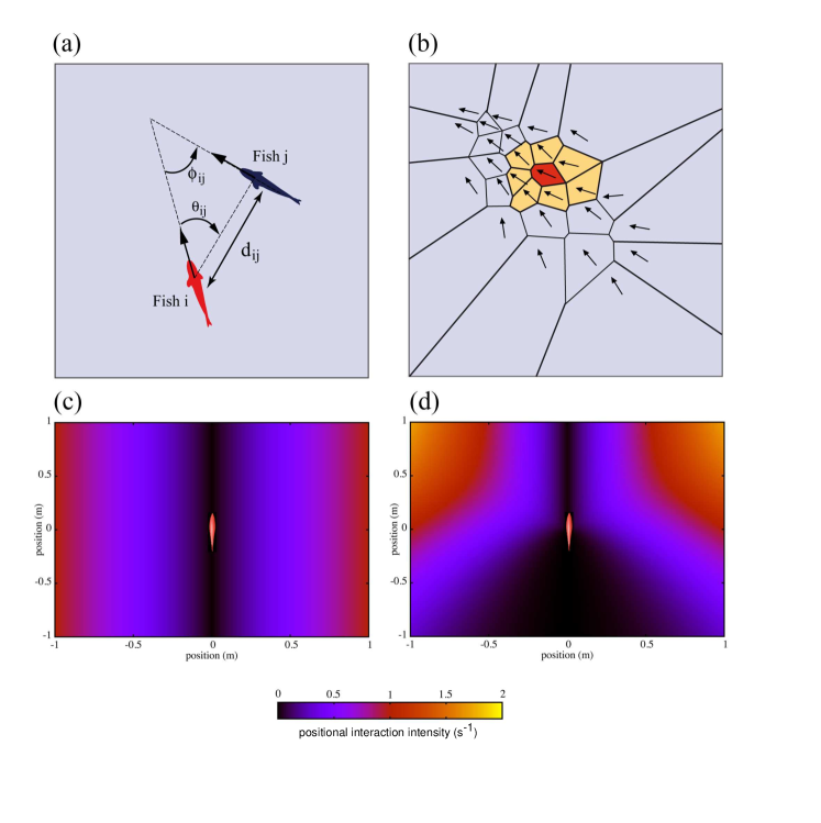
Figure 1: Fish interactions graphical representation used in the model. $(a)$ The distance $d_{ij}$ of fish $j$ from fish $i$; $\phi_{ij}$ is the relative orientation heading of fish $j$ compared to fish $i$; $\theta_{ij}$ is the angle between the angular position of fish $j$ with respect to fish $i$. $(b)$ illustration of the Voronoi neighbourhood, where arrows indicate the fish headings of the focal fish (red region) to his first Voronoi neighbours (yellow regions). $(c)$ Positional interaction intensity as proposed by Gautrais et al $(d)$ Positional interaction intensity as given by the new angular preference.

In the above equation, $\omega^{*}(t)$ is the stimulus/response function based on the individuals response to the proximity of the tank wall —irrelevant in the following as we shall consider groups evolving in an infinite domain— and on the reaction to the neighbouring fish orientation and distance. It was found that for groups of two fish, these social interactions are well described by a linear superposition of alignment and attraction with weights depending on $d_{ij}$, the distance between the two fish. It was found further that in groups of more than two fish, many-body interactions could be safely approximated by the normalized sum of pair interactions with those individuals forming the first shell of Voronoi neighbours of the focal fish (figure 1). Mathematically, one has:

$$\omega^{*}=\frac{1}{N_{i}}\sum_{j\in V_{i}}\left[k_{V}\,v\,\sin\phi_{ij}+k_{P}\,d_{ij}\,\sin\theta_{ij}\right]$$ (2)

where $V_{i}$ is the Voronoi neighbourhood of fish $i$ containing $N_{i}+1$ individuals, $\phi_{ij}=\phi_{j}-\phi_{i}$ is the angle between the orientational headings of fish $i$ and $j$, and $\theta_{ij}$ is the angle between the heading of fish $i$ and the vector linking fish $i$ to fish $j$ (figure 1). The functional forms involving the sine function, chosen for simplicity, were also validated by the data. They ensure that interactions vanish when the fish are already aligned or in front of each other as can be seen in figure 1$(c)$.

Note there is a speed dependence with the alignment, and hence a tendency to produce polarised groups at large speeds. A similar positive correlation between group speed and polarity has also been found in groups of giant Danios (Devario aequipinnatus) and golden shiners (Notemigonus crysoleucas) [21, 22].

Note also that the strength of the attractive positional interaction, scaled by $k_{P}$ , increases linearly with $d_{ij}$, which is rather unrealistic: if two fish were very far apart, they would turn at extremely large speeds towards each other. Moreover, attraction is of the same amplitude whether fish $j$ is in front or behind fish $i$, which may also look unrealistic, as one might expect fish $i$ to be less “aware” and attracted to fish $j$ if $j$ is behind $i$. Nevertheless this form of attraction interaction was found to account well for the data, because (i) in the experimental tank fish never go far away from each other; (ii) data were too scarce to allow for detecting a frontal preference. In the following, we restrict ourselves to moderate-size groups, so that the fish inter distances remain rather small, and we could thus keep the unbounded expression of the positional interaction strength. However, we will consider the possibility of an angular weighting of the interactions in the form of an extra multiplicative factor

$$\Omega_{ij}=1+\cos(\theta_{ij})$$ (3)

to the interaction term $\omega^{*}(t)$, so that (1) is rewritten as:

$$\,\mathrm{d}\omega(t)=-v\left[\frac{\,\mathrm{d}t}{\xi}\left(\omega(t)-\Omega_{ij}\omega^{*}(t)\right)+\sigma\,\mathrm{d}W\right],$$ (4)

The function $\Omega_{ij}$ was designed to ensure a frontal preference and some kind of rear blind angle. Its specific form (which can be seen in figure 1$(d)$) was chosen for its simplicity and its unit angular average.

In the following, we perform numerical simulations of the model, varying its key parameters: the swimming speed $v$, and $k_{P}$ and $k_{V}$, the behavioural parameters controlling attraction and alignment. Most of our study is restricted to moderate-size groups of $N=100$ fish. However, we also present results as a function of group size when investigating the robustness of milling (section 6). Typically, a set of 100 random initial conditions is simulated over a period of 1000 seconds, where the first half of each series was discarded to account for transient behaviour.

The polarisation of the school is quantified by the global polar order parameter

$$P=\frac{1}{N}\left|\sum_{i=1}^{N}\frac{\vec{v}_{i}}{v}\right|$$ (5)

which reaches order 1 values for strongly polarised, schooling groups. Milling behaviour is detected via the global normalised angular momentum

$$M=\frac{1}{N}\left|\sum_{i=1}^{N}{\frac{\vec{r}_{i}\times\vec{v}_{i}}{|\vec{r}_{i}|v}}\right|$$ (6)

which will tend towards unity when the school is rotating in a single vortex. As we shall see, the two scalar, positive, quantities $P$ and $M$ often play symmetric roles in the ordered phases of the groups: a schooling group will show large $P$ and negligible $M$, and the opposite is true for a milling group.

3 Speed-induced transition to schooling

We first report the basic transition from swarming to schooling observed when increasing the swimming speed of individuals. Already observed in [1], it is the natural consequence of the predominance of the alignment interaction at high speeds. Here, we confirm the existence of the transition in the absence of walls confining the group. Figure 2 summarises our results for $N=100$ individuals, using the parameter values determined from the experimental data obtained in smaller groups ( $k_{V}$ = 2.7 m^-1, $k_{P}$ = 0.41 m^-1s^-1, $\xi$ = 0.024 m and $\sigma$ =28.9 m^-1s^-1/2), with and without the angular preference function $\Omega$.

We find that the transition to schooling occurs at a speed range of zero to four body lengths per second, a reasonable one considering the barred flagtail swimming ability (figure 2$(a)$). The transition is smoother with angular preference (red curves) and consequently requires larger speed values to reach similar results as the original model. Even though no pronouced milling is found in either cases of figure 2$(b)$, a more pronounced result is achieved with the angular preference, which seems to directly influence the school distance to the centroid on figure 2$(c)$.

4 Dedimensionalisation of the model

In order to get more insight into how speed affects the relative importance of noise, directional and positional behavioural reactions, we rewrite the model in a dedimensionalized form. After a straightforward manipulation we are left with only three independent parameters:

$$\alpha=\xi^{3}\sigma^{2}/v,\;\;\;\beta=(k_{V}v)/(\xi^{2}\sigma^{2}),\;\;\;{\rm and}\;\;\gamma=(k_{P}v)/(\xi^{4}\sigma^{4})\;.$$ (7)

The time step $\,\mathrm{d}\tilde{t}=\,\mathrm{d}t/(\xi^{2}\sigma^{2})$ has no influence on the simulations provided it is small enough. For all simulations we used a $\,\mathrm{d}\tilde{t}=0.1\alpha$ for $\alpha<0.1$ or $\,\mathrm{d}\tilde{t}=0.01$ for the remaining cases. The full set of dedimensionalised equations reads:

$$\alpha\,\mathrm{d}\tilde{\omega}(\tilde{t})=\,\mathrm{d}\tilde{t}\left(\tilde{\omega}(\tilde{t})-\tilde{\omega}^{*}(\tilde{t})\right)+\,\mathrm{d}W,$$ (8)

where $\,\mathrm{d}W$ refers to a standard Wiener process. The term $\tilde{\omega}^{*}$ rewrites as:

$$\tilde{\omega}^{*}=\frac{1}{N_{i}}\sum_{j\in V_{i}}\left[\beta\sin\phi_{ij}+\gamma\,\tilde{d}_{ij}\,\sin\theta_{ij}\right].$$ (9)

Note that in our equivalent system, time is now counted in units of a typical time $\tilde{x}=v(\xi\sigma)^{-2}$, defined with the correlation length $\xi$ and noise amplitude $\sigma$. The distance is expressed in units of a typical length $\tilde{x}=v(\xi\sigma)^{-2}$, which is simply the displacement of a fish during time $\tilde{t}$ with speed/velocity $v$. The angular speed and thus the evolution of the fish orientation are determined by the relative weight of equivalent alignment ($\beta$) and positional ($\gamma$) intensity over the equivalent angular inertia term $\alpha$.

The expressions of the dedimensionalized coefficients show that increasing speed, while keeping other parameters constant, leads to an increase in the equivalent positional and alignment interactions. At the same time it reduces the angular inertia while keeping the equivalent noise amplitude/intensity constant. The speed induced transition can thus be seen as a competition between noise and social interactions.

Hereafter we perform an extensive study of the dedimensionalised version of the model, with particular attention paid to the emergence of significant milling.

5 Phase diagram in the space of behavioural parameters

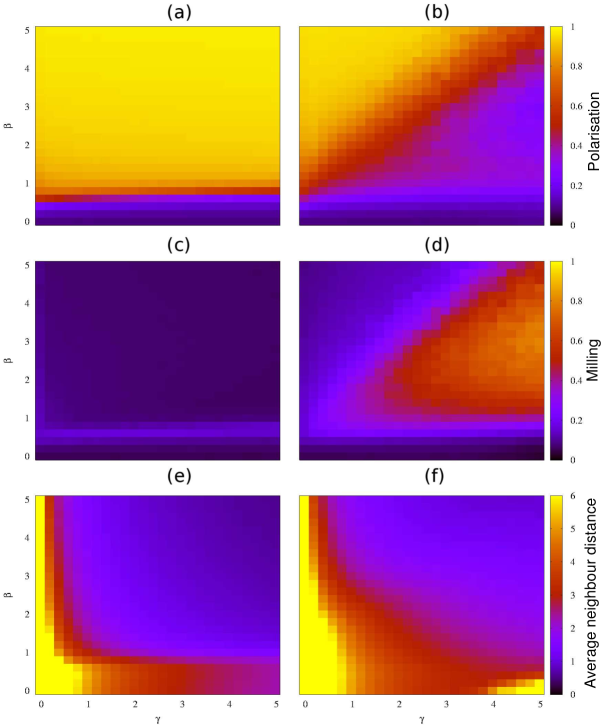
Figure 3: Statistics for simulations made for different alignment and positional parameters ($\beta$ and $\gamma$ respectively), both in the interval [0,5] with an increment of 0.2 (in both $\beta$ and $\gamma$ units respectively). Simulations were made with an angular inertia term of $\alpha\approx 0.014$ (equivalent to a speed $v=0.8{\rm m/s}$). The colour code bar on the right represents the values for the respective statistics on the left (polarisation, milling and average distance to the neighbours). The left column represents different statistics for the original model as seen in (1), while the right column graphs represent simulations with the new angular preference as seen in (4). The statistics here represented are: $(a)$ and $(b)$ polarisation parameter; $(c)$ and $(d)$ milling parameter; $(e)$ and $(f)$ the average neighbour distance. Each data point is the result of an average over 100 different simulations, where the first half of each simulation was discarded to avoid transional behaviours, resulting in a total of 2$\times 10^{6}$ data points for every parameter configuration.

We explored the parameter plane formed by coefficients $\beta$ and $\gamma$ in the domain $[0,5]\times[0,5]$ including the experimentally-determined values $k_{V}$ = 2.7 m^-1 ($\beta\approx 2.24$) and $k_{P}$ = 0.41 m^-1s^-1 ($\gamma\approx 0.71$) by steps of 0.2, yielding the $26\times 26$ grid of results shown in figure 3. The angular inertia term was set at $\alpha\approx 0.014$, equivalent to the experimentally reasonable value $v=0.8{\rm m/s}$.

Two cases are presented, without and with the angular weighting function $\Omega$ (left and right panels respectively). In both cases, a transition to schooling is observed as $\beta$ is increased (figures 3$(a$) and 3$(b)$). Such a transition is virtually independent of $\gamma$ considering the original model (figure 3$(a)$) while presenting a functional form for simulations using the new angular dependence (figure 3).

A strong qualitative difference is nevertheless observed between the left and the right panels in figures 3$(c)$ and 3$(d)$. With the angular dependence $\Omega$ (right panels), outright schooling is preceded by a large region where milling is observed (3$(d)$), whereas no significant milling occurs without angular weighting (3$(c)$). This may not seem too surprising given that $\Omega$ favours the formation of (local) files in which fish follow those in front of them.

Lastly, we observe a peculiar property in figures 3$(e)$ and 3$(f)$, which show the average distance to neighbours. With the angular preference (figure 3$(f)$), the region of low $\beta$ exhibits a weak ridge bordering the swarming region ($\gamma$ and $\beta\approx 0$) where the average distance is expected to diverge. This ridge extends to high $\gamma$ values for which one would infer small-size schools and shorter neighbour distances. One should be aware that the colour code presented on these last two figures interpret values above the range [0,6] all as having the same colour (yellow). This was introduced since a divergence occurs in the swarming region, but this unfortunately masks secondary ridges, such as the one found in figure 3$(f)$. Similar regions may be found in figure 3$(e)$, although masked by the swarming region divergence in this visualization.

The explanation, despite being initially counter intuitive, is rather simple. Despite the $\gamma$-induced tendency to stay together, a low $\beta$ means that fish have a lower tendency to disturb their alignment to match that of their neighbours, meaning that fish will rely mostly on the positional interaction. This implies that if a neighbour is directly ahead or behind the focal fish, there is no need to change the direction of motion. Also, both cases (with or without the new angular preference) have a zero interaction for anti-parallel neighbours. This means that when $\gamma$ dominates the interactions, the stable fish configuration is a line. Having noise in (1) or (4) leads to fish organizing themselves in a quasi-unidimensional configuration, and the fish in front, not having additional neighbours on their sides, will eventually turn due to noise. After a slight turn, this fish will now have new Voronoi neighbours, with fish previously located behind it now located slightly to its side, and make a 180 degree turn to recover the optimal configuration. This mechanism leads fish to organize themselves in two columns going in opposite directions connected at the end of the school by this “U turn” (see snapshot in figure 4$(c)$, panel III).

To visualize the above results in a synthetic way, we took advantage of the fact that the main behavioural regions apparent in figures 3$(b)$, 3$(d)$ and 3$(f)$ are distinguished by mutually-exclusive quantities: when schooling is strong, milling is weak and the distance to neighbours ($D$) is small; when milling is strong, schooling is weak, and $D$ is small; when $D$ is larger, both schooling and milling are weak. This mutual exclusion of schooling and milling is clear in the time series shown in figure 4$(a)$. We thus constructed the following composite order parameter:

$$S(P,M,D)=P+M\exp[i2\pi/3]+D\exp[i4\pi/3]$$ (10)

which takes complex values such that the phase codes for the behaviour and the modulus for the intensity of this behaviour, where the average distance was normalised according to the largest value observed. As a result, the information of the right panels of figure 3 is represented synthetically in figure 4$(b)$. Three distinct regions are clearly apparent as each is represented in a different colour (red for polarisation, blue for milling and green for average neighbour distance). Typical configurations of the group corresponding to the time-series of figure 4$(a)$ are shown in figure 4$(c)$. (See also the movies in the supplementary material A.1 to A.4 for simulations of these 4 behaviours.)

Regions I and II refer to the schooling and milling states respectively. Region III refers to the winding (line configuration) state mentioned previously. It could be argued that regions II and III are similar, having only changed the width/length ratio. Nevertheless region III has very weak rotational behaviour at odds with full blown milling. Note finally the intermittence between schooling and milling in the transition region between regions I and II.

Finally, we come back to the effect of the swimming speed. The above analysis in the $(\beta,\gamma)$ plane was repeated at different values of $\alpha$ corresponding to speed values of 0.4, 0.8 and 1.2 m/s, building a three-dimensional phase diagram. In figure 5 we show that these transition lines superimpose onto a master curve delimiting the schooling and milling zones. Thus, no qualitative changes were observed for these values of $\alpha$, indicating the robustness of the phase diagram in figure 4 for speeds in the experimental range. We studied this phase boundary marking the transition, via intermittent regimes, between schooling and milling more quantitatively. Defining the transition points as those where both the polarisation and milling parameters spend more than 40 percent of the time above the threshold value of 0.8, we find that the transition line, for all values of $v$ studied, can be fitted by the simple functional form

$$\beta=A\sqrt{\gamma}+B$$ (11)

where $A$ and $B$ take values independent of $\alpha$ in the ranges studied (figure 5).

Although we do not have a quantitative explanation for the above functional form, these fits indicate the possibility of a rather simple theory accounting for the full phase diagram of our model. Meanwhile a qualitative explanation for the dependence on $\gamma$ is given by the need to counteract the global polarisation tendency given by $\beta$, while maintaining a local one. Also, figure 3$(a)$ indicates minimum $\beta\times\gamma$ values to overcome the noise. In the supplementary material there are 2 videos (A.6 and A.5) of the two dimensional histogram evolution for the schooling and milling parameters as we change $\beta$ or $\gamma$ while maintaining the other one constant ( $\gamma=17.28$ and $\beta=13.30$), meaning we have respectively vertical and horizontal transition cross-sections in figure 5.

6 Group-size-induced transition

In this section, we investigate the influence of group size on the robustness of both milling and schooling behaviour in our model using the angular weighting function. Apart from the general theoretical context mentioned above, this is also of direct relevance for fish, as it has been reported recently that in golden shiners increasing group size significantly increases the amount of time spent in a milling state [22].

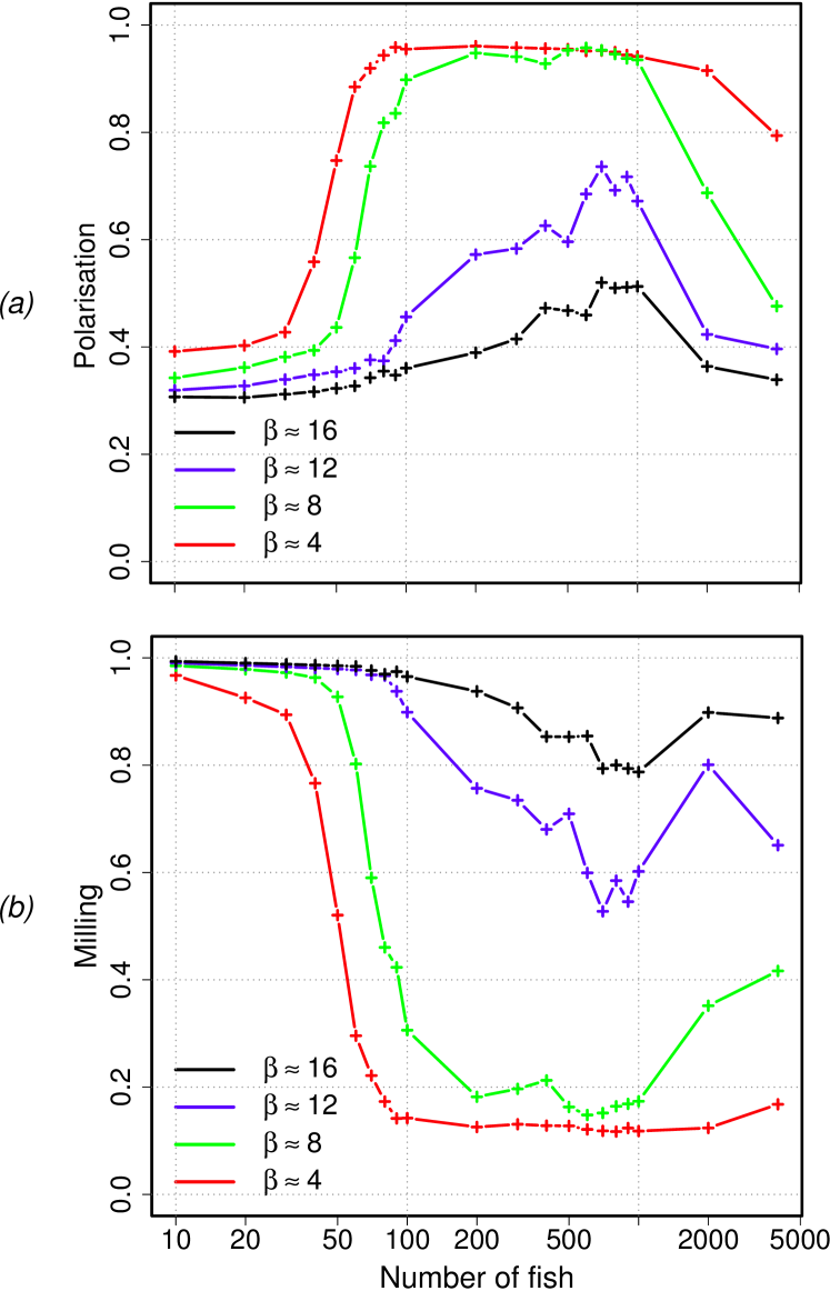
Figure 6: Simulations done for a fixed $\gamma\approx 4.5$ with an angular inertia term of $\alpha\approx 0.014$ (equivalent to a speed $v=0.8{\rm m/s}$) for different quantities of fish and $\beta$ values, where $(a)$ and $(b)$ refer to the milling and polarisation parameter respectively.

We performed a series of simulations at fixed $\gamma\approx 4.5$ with an angular inertia term $\alpha\approx 0.014$ (equivalent to a speed $v=0.8{\rm m/s}$). Figure 6 shows the milling and schooling order parameters for simulations of groups from 10 to 4000 fish. These results indicate that there exists an inferior limit of approximately 60 fish in order to achieve significant milling and that this behaviour progressively disappears at large sizes. Although these results must be taken with care given the unbounded character of the variation of positional interaction with distance to neighbours, they show that for up to 100 fish, increasing group size induces a transition from schooling to milling for $\beta\leq 8$. For larger values of the alignment parameter, despite having higher overall values for the milling parameter, the transition does not occur. This indicates that in the model studied here, like in many of those proposed before [23], milling dynamics does not emerge in the arbitrarily large infinite-size limit.

Although such a statement has obvious interest for physicists, we believe it bears some importance regarding animal group behaviour. Also, it is worth noting that the variation on the milling parameter seen for $\beta\geq 12$ in figure 6$(a)$ happens as the duration of the milling and schooling behaviour increases with $N$. Such an increase is so intense that for simulations with more than 300 fish, usually only one behaviour can be seen for every initial condition, giving a very large standard deviation and a highly fluctuating average. Furthermore, some simulations for $N>1000$ displayed more than one vortex at the same time, patterns which the milling parameter cannot account for. One can see in figure 6$(b)$ that the schooling behaviour is affected by the size as well. This again is due to the effect of large schools. This stretch on school extensions enables information propagation delays, which in turn, cause reductions on the global polarisation parameter. It is easy to see how a three dimensional configuration could achieve lower extensions with large fish quantities, which would in turn minimise these effects.

7 Conclusions

Understanding how complex motion patterns in fish schools arise from local interactions among individuals is a key question in the study of collective behaviour [24, 25]. In a previous work, Gautrais et alhave determined the stimulus/response function that governs an individual’s moving decisions in Barred flagtail (Kuhlia mugil) [1]. It has been shown that two kinds of interactions controlling the attraction and the alignment of fish are involved and that they are weighted continuously depending on the position and orientation of the neighboring fish. It has also been found that the magnitude of these interactions changes as a function of the swimming speed of fish and the group size. The consequence being that groups of fish adopt different shapes and motions: group polarisation increases with swimming speed while it decreases as group size increases.

Here we have shown that the relative weights of the attraction and alignment interactions play a key role in the emergent collective states at the school level. Depending on the magnitude of the attraction and the alignment of fish to their neighbours, different collective states can be reached by the school. The exploration of the parameter space of the Gautrais et al model reveals the existence of two dynamically stable collective states: a swarming state in which individuals aggregate without cohesion, with a low level of polarisation, and a schooling state in which individuals are aligned with each others and with a high level of polarisation. The transition between the two states is induced by an increase of the swimming speed. Furthermore, the addition in the model of a frontal preference to account for the angular weighting of interactions leads to two other collective states: a milling state in which individuals constantly rotate around an empty core thus creating a torus and a winding state, in which the group self-organises into a linear crawling structure. This last group structure is reminiscent of some moving patterns observed in the Atlantic herring (Clupea harengus) [26].

Of particular importance is the transition region between milling and schooling. In this region, the school exhibits multistability and it regularly shifts from schooling to milling for the same combination of individuals’ parameters. This particular property was recently reported in experiments performed in groups of golden shiners [22]. Our results show that the transition region can be described by a simple functional form describing the respective weights of the alignment and attraction parameters and is independent of the fish swimming speed in the experimental range. The modulation of the strength of the alignment and attraction may depend on the behavioural and physiological state of fish [27]. In particular, various environmental factors such as a perceived threat may change the way fish respond to their neighbours and hence lead to dramatic changes in collective motion patterns at the school level [28, 29].

Finally, we show that collective motion may dramatically change as group size increases. The absence of a milling state in the largest groups is a natural consequence of the spatial constraints exerted upon individuals’ movements as the number of fish exceeds some critical value. These constraints could be much less stringent in 3D, as testified by the observation of cylindrical vertical milling structures involving several thousands of fish in bigeye trevally (Caranx sexfasciatus). With an additional dimension, the same number of fish could result into a mill of much smaller diameter, not only avoiding the problems of distance dependence, but also minimizing information propagation delays and the emergence of competing behaviours.

A more in depth physics study of the transitions presented here is necessary. Unfortunately the present model is restricted to schools of biologically-relevant sizes ($N\approx 100$ fish) preventing such analysis for the current social interactions. In this manner, additional changes to the model are required, among them are: i) eliminating the linear distance dependence on the interactions, by either implementing a saturation or a decay to this interaction; ii) changing the boundary conditions for periodic ones to avoid evaporating schools once the distance dependence is removed; iii) a three dimensional study of the model to check the impact of an additional level of freedom on the school behaviour.

8 Acknowledgements

We are grateful to Jacques Gautrais and Sepideh Bazazi for comments on the manuscript. Daniel S. Calovi was funded by the Conselho Nacional de Desenvolvimento Científico e Tecnológico - Brazil. Ugo Lopez was supported by a doctoral fellowship from the scientific council of the Université Paul Sabatier. This study was supported by grants from the Centre National de la Recherche Scientifique and Université Paul Sabatier (project Dynabanc).

9 References

10 Figures

Figure 2: $(a)$ Displays the polarisation parameter as a function of the speed $v$, for simulations with the original model (blue) and the new angular preference (red), where a collective state transition to schooling can be seen in both cases, although more abruptly in the original model (blue line). $(b)$ milling parameter for both simulations (blue original model and red with the new angular preference) as a function of the speed. One observes that in the transition zone ($v\approx$ 0.2 m/s) there is an increase in milling values in the new angular preference simulations (red). $(c)$ average distance to the neighbours for both sets of simulations. We performed 10 replicates for each different speed, and all simulations were had $10^{7}$ iterations, where we discarded the first half of data, and used only one datapoint for every 10 iterations.

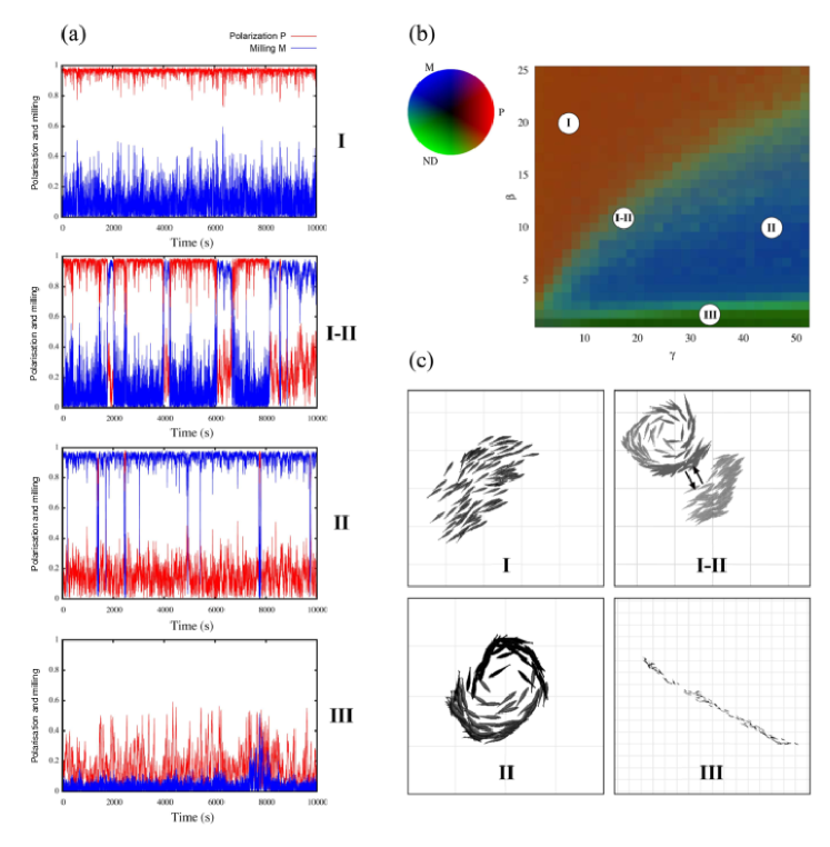
Figure 4: $(a)$ The respective time series of the polarisation (red line) and milling parameters (blue line) for the four distinct regions. $(b)$ is a representation of figure 3 right panels where distinct behavioural regions can be identified. $(c)$ typical configurations of these states.

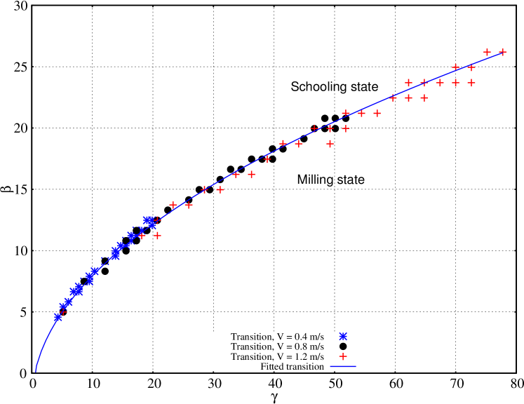
Figure 5: Transition between region schooling and milling states for different speeds. A functional form ($A\sqrt{\gamma}+B$) fitted for $v$ = 0.8 m/s proved to also properly describe the transitions for speeds of 0.4 and 1.2 m/s, where $A=3.22\pm 0.05$ and $B=-2.23\pm 0.26$. in order to better

Appendix A Supplementary information

Supplementary Material A.1: Region_I.avi - Simulation with 100 fish made on the schooling parameter space region as seen in figure 4$(b)$. Note the data was post-treated so that the simulations seem to have been made with periodic boundary conditions. This representation was chosen in order to have an easier visualisation of the group dynamics, but all simulations were performed in an infinite spatial domain.

Supplementary Material A.2: Region_II.avi - Simulation with 100 fish made on the milling parameter space region as seen in figure 4$(b)$. Note the data was post-treated so that the simulations seem to have been made with periodic boundary conditions. This representation was chosen in order to have an easier visualisation of the group dynamics, but all simulations were performed in an infinite spatial domain.

Supplementary Material A.3: Region_I-II.avi - Simulation with 100 fish made on the transition between schooling and milling parameter space region as seen in figure 4$(b)$. Note the data was post-treated so that the simulations seem to have been made with periodic boundary conditions. This representation was chosen in order to have an easier visualisation of the group dynamics, but all simulations were performed in an infinite spatial domain.

Supplementary Material A.4: Region_III.avi - Simulation with 100 fish made on the line parameter space region as seen in figure 4$(b)$. Note the data was post-treated so that the simulations seem to have been made with periodic boundary conditions. This representation was chosen in order to have an easier visualisation of the group dynamics, but all simulations were performed in an infinite spatial domain.

Supplementary Material A.5: Gamma.avi - Two dimensional histogram evolution for the schooling and milling parameters as we change $\beta$ while maintaining $\gamma=17.28$, meaning a vertical cross section on the transition represented on figure 5.

Supplementary Material A.6: Beta.avi - Two dimensional histogram evolution for the schooling and milling parameters as we change $\gamma$ while maintaining $\beta=13.30$, meaning a horizontal cross-section on the transition represented on figure 5.

References

- [1] J. Gautrais, F. Ginelli, R. Fournier, S. Blanco, M. Soria, H. Chaté, and G. Theraulaz. Deciphering interactions in moving animal groups. PLoS Comput. Biol., 8(9), 2012.
- [2] I.D. Couzin and J. Krause. Self-organization and collective behavior in vertebrates. Adv. Stud. Behav., 32:1–75, 2003.
- [3] D.J.T. Sumpter. Collective animal behavior. Princeton, N.J. : Princeton University Press, 2010. Includes bibliographical references and index.
- [4] R.V. Solé. Phase transitions. Princeton University Press, Princeton, NJ, 2011.
- [5] D.V. Radakov. Schooling in the ecology of fish. J. Wiley, 1973.
- [6] T.J. Pitcher. Behavior of Teleost Fishes. Fish and Fisheries Series. Chapman & Hall, 1993.
- [7] J.K. Parrish and L. Edelstein-Keshet. Complexity, pattern, and evolutionary trade-offs in animal aggregation. Science, 284(5411):99–101, 1999.
- [8] P. Freon and O.A. Misund. Dynamics of Pelagic Fish Distribution and Behaviour: Effects on Fisheries and Stock Assessment. Fishing News Books. Wiley, 1999.
- [9] J.K. Parrish, S.V. Viscido, and D. Grunbaum. Self-organized fish schools: An examination of emergent properties. Biol. Bull, 202(3):296–305, 2002. Workshop on the Limitations of Self-Organization in Biological Systems, Marine Biol Lab, Woods Hole, Massachusetts, May 11-13, 2001.
- [10] Ch. Becco, N. Vandewalle, J. Delcourt, and P. Poncin. Experimental evidences of a structural and dynamical transition in fish school. Physica A, 367(C):487–493, 2006.
- [11] I. Aoki. A simulation study on the schooling mechanism in fish. B. JPN Soc. Sci. Fish, 48(8):1081–1088, 1982.
- [12] I.D. Couzin, J. Krause, R. James, G.D. Ruxton, and N.R. Franks. Collective memory and spatial sorting in animal groups. J. Theor. Biol., 218(5):1–11, 2002.
- [13] T. Vicsek, A. Czirók, E. Ben-Jacob, I. Cohen, and O. Shochet. Novel type of phase transition in a system of self-driven particles. Phys. Rev. Lett., 75:1226–1229, 1995.
- [14] A. Czirók, H.E. Stanley, and T. Vicsek. Spontaneously ordered motion of self-propelled particles. J. Phys. A-Math. Gen., 30(5):1375, 1997.
- [15] H. Chaté, F. Ginelli, G. Grégoire, and F. Raynaud. Collective motion of self-propelled particles interacting without cohesion. Phys. Rev. E, 77(4):046113, 2008.
- [16] J.P. Newman and H. Sayama. Effect of sensory blind zones on milling behavior in a dynamic self-propelled particle model. Phys. Rev. E, 78(1):011913, 2008.
- [17] S. Mishra, K. Tunstrøm, I.D. Couzin, and C. Huepe. Collective dynamics of self-propelled particles with variable speed. Phys. Rev. E, 86(1):011901, 2012.
- [18] P. Szabó, M. Nagy, and T. Vicsek. Turning with the others: novel transitions in an spp model with coupling of accelerations. In Self-Adaptive and Self-Organizing Systems, 2008. SASO’08. Second IEEE International Conference on, pages 463–464. IEEE, 2008.
- [19] J. Gautrais, C. Jost, M. Soria, A. Campo, S. Motsch, R. Fournier, S. Blanco, and G. Theraulaz. Analyzing fish movement as a persistent turning walker. J. Math. Biol., 58:429–445, 2009.
- [20] G.E. Uhlenbeck and L.S. Ornstein. On the theory of the brownian motion. Physical Review, 36:823–841, 1930.
- [21] S.V. Viscido, J.K. Parrish, and D. Grunbaum. Individual behavior and emergent properties of fish schools: a comparison of observation and theory. Mar. Ecol-Prog Ser., 273:239–249, 2004.
- [22] K. Tunstrøm, Y. Katz, C.C. Ioannou, C. Huepe, M.J. Lutz, and I.D. Couzin. Collective states, multistability and transitional behavior in schooling fish. PLoS Comput. Biol., 9(2), 2013.
- [23] R. Lukeman, Yue-Xian Li, and L. Edelstein-Keshet. A Conceptual Model for Milling Formations in Biological Aggregates. B. Math. Biol., 71(2):352–382, 2009.
- [24] U. Lopez, J. Gautrais, I.D. Couzin, and G. Theraulaz. From behavioural analyses to models of collective motion in fish schools. Interface Focus, 2(6):693–707, 2012.
- [25] J. Delcourt and P. Poncin. Shoals and schools: back to the heuristic definitions and quantitative references. Rev. Fish Biol. Fisher., 22(3):595–619, 2012.
- [26] F. Gerlotto, Bach P., Bertrand A., Bertrand S., Brehmer P., Cotel P., Dagorn L., Fréon P., Girard C., Josse E., and Soria M. Towards a synthetic view of the mechanisms and factors producing the collective behavior of tropical pelagic fish : individual, school, environment and fishery. In Proceedings of the ICES Symposium on Fish Behaviour in Exploited Ecosystems, Bergen, Norway, 2003.
- [27] S.E. Wendelaar Bonga. The stress response in fish. Physiol. Rev., 77(3):591–625, 1997.
- [28] J.A. Beecham and K.D. Farnsworth. Animal group forces resulting from predator avoidance and competition minimization. J. Theor. Biol., 198(4):533–548, 1999.
- [29] S.V. Viscido and D.S. Wethey. Quantitative analysis of fiddler crab flock movement: evidence for ‘selfish herd’ behaviour. Anim. Behav., 63(4):735–741, 2002.