Non-equilibrium finite temperature dynamics of magnetic quantum systems: Applications to spin-polarized scanning tunneling microscopy

Abstract

We calculate the real time non-equilibrium dynamics of quantum spin systems at finite temperatures. The mathematical framework originates from the $C^{*}$-approach to quantum statistical mechanics and is applied to samples investigated by means of spin-polarized scanning tunneling microscopy. Quantum fluctuations around thermal equilibrium are analyzed and calculated. The time averaged expectation values agree with the time averaged experimental data for magnetization curves. The method is used to investigate the dynamics of a sample for shorter times than the resolution time of the experimental setup. Furthermore, predictions for relaxation times of single spins on metallic and semiconductor surfaces are made. To check the validity of our model we compare our results with experimental data obtained from Fe adatoms on InSb and Co adatoms on Pt(111) and find good agreement. Approximated thermalization is found numerically for the expectation values of the spin operators.

I Introduction

Spin sensitive studies of individual magnetic adatoms and atomic ensembles on surfaces with spin-polarized scanning tunneling microscopy (SP-STM) WiesendangerAnfang ; Wiesendanger:RMP2009 have raised the necessity of a quantum-mechanical description of the spin dynamics evoked by SP-STM experiments. Magnetization curves obtained in experiments are typically described using the expectation values of observables using a time independent, i.e. kinematic, Gibbs ensemble average Meier:Science(2008) ; Kha:Nature2010 . However, an SP-STM measurement is a time-average of the orientation of a spin component selected by the given spin orientation of the probe tip. Therefore, the dynamics of the magnetization in the sample under the study remains unknown within the experimental resolution time. It would be helpful to compensate this lack of knowledge with theoretical investigations.

When the STM tip comes towards an atom or a cluster under the study, the Hamilton operator of the system changes due to the interactions with tunneling electrons. The perturbed dynamics drives the state out of equilibrium and the ergodicity is not a priory ensured. Therefore, the ergodicity of a system has to be checked for a reliable interpretation of experimental results. A still unexplained finding is the extremely high switching frequency of Co atoms on Pt(111) at zero magnetic field Meier:Science(2008) . In contrast to magnetic atoms on insulating substrates Co/Pt(111) possesses very strong out-of-plane anisotropy (9 meV) without any transversal contributions. Hence, the Hamiltonian of the free system is diagonal in the $|S_{z}\rangle$ basis and, therefore, the tunneling rate is zero Meier:Science(2008) . The anisotropy barrier is approximately 100 times larger than the temperature used in experiments. Therefore, the Boltzmann probability to pass this barrier by thermal activation is also negligible. The measured magnetization, in contrast, is zero at zero field even in the regime of elastic tunneling, where the tunneling current density is minimal. A related problem is the so-called ”return to equilibrium”, also referred as relaxation. The relaxation of an excited system depends on its initial state Bratelli . There might exist some initial states from which the system can return to equilibrium and there might exist some other initial states from which this process will not happen.

The formal, mathematical description of systems which can be described by different Hamilton operators before/after and during the measurement process has been elaborated in the framework described in Bratelli . The algebraic approach to quantum statistical mechanics provides appropriate mathematical tools to verify the dynamical relaxation of a disturbed system (return to equilibrium) analytically Bratelli ; ArakiI ; ArakiII . Several theoretical aspects in the algebraic approach to quantum spin systems, such as propagation velocities, are of actual research interest NachtergaeleI -NachtergaeleIIIIIII . Particularly, it is proven that a mathematically exact return to equilibrium is ensured if the dynamical system satisfies some form of asymptotic abelianness and if the initial state is a perturbed KMS state (Kubo-Martin-Schwinger) Bratelli . In the present paper we use the algebraic formulation of quantum statistical mechanics Bratelli to clearly separate the thermal equilibrium Gibbs states and the time evolution of the system during SP-STM experiments.

It is generally believed, that only large systems show a relaxation process. We demonstrate that also expectation values of relatively small quantum spin systems, containing less than 10 particles, return approximately to equilibrium when a perturbed KMS state is used as an initial state. Especially interesting is the theoretical analysis of the dynamics on time scales which are not accessible for an STM. Using exact diagonalization we calculate the dynamics of single quantum spins during and after SP-STM measurements at finite temperatures. We demonstrate that the relaxation times of those quantum objects on different substrates lie in the femto-, pico- or nanosecond regime. It means that a good approximation of the long time behavior can be given for certain classes of real finite systems. To check whether the short time dynamics has a reliable behavior, the calculated relaxation time has been compared with experimentally determined life times for single spins Kha:Nature2010 . Ground states are obtained from KMS states if the zero temperature limit is performed.

II Method

The SP-STM set-up is approximated by (in general) two different Hamiltonians in our approach. There is a Hamiltonian $H$ for the free system and, if a measurement is started, we get an additional hermitian operator $P$ for the interaction between the tip and the sample. Hence, if the tip is moved towards the surface, the system switches from $H$ to $H+P$ because of the sudden emergence of tunneling electrons causing the interaction between the tip and the sample.

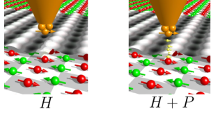
Figure 1: $H$ describes the free system and $H+P$ describes the perturbed system, i.e. the system with interaction between the tip and the sample.

The STM-tip can be used to prepare a system with desired expectation values. For the corresponding state we choose a perturbed KMS state $\omega^{\beta P}$. The reason for the application of this state is justified in the following text.

To describe a quantum spin system we consider particles on a lattice $\mathbb{Z}^{d}$ and associate with each point $x\in\mathbb{Z}^{d}$ a Hilbert space $\mathcal{H}_{x}$ of dimension $2s(x)+1$. With a finite subset $\lambda\subset\mathbb{Z}^{d}$ we associate the tensor product space $\mathcal{H}_{\lambda}=\bigotimes_{x_{i}\in\lambda}\mathcal{H}_{x_{i}}$. The local physical observables are contained in the algebra of all bounded operators acting on $\mathcal{H}_{\lambda}$. This is the $C^{*}$-algebra $\mathcal{A}_{\lambda}\cong\bigotimes_{x_{i}\in\lambda}M_{2s(x_{i})+1}$ in which $M_{n}$ denote the algebra of $n\times n$ complex matrices. Physically, this can be interpreted as follows: at each lattice site $x$ there is a particle with spin quantum number $s(x)$ and with $n=2s(x)+1=dim(\mathcal{H}_{x})$ degrees of freedom. The numerical calculations are done for systems of finite dimensions. The indices $x$, $x_{i}$ and $\lambda$ are suppressed in the following text for clarity. A mixed (or normal) state $\omega$ is described as a normalized positive linear functional over the matrix algebra $\mathcal{A}$ and is given by a density matrix $\rho$.

$$\omega:\mathcal{A}\rightarrow\mathbb{C},\quad A\mapsto\omega(A)=Tr(\rho A)$$ (1)

The dynamical evolution of an observable $A\in\mathcal{A}$ for a system with Hamiltonian $H=H^{*}\in M_{n}$ can be described by the Heisenberg relations

$$\tau_{t}:\mathcal{A}\rightarrow\mathcal{A},\quad A\mapsto\tau_{t}(A)=e^{\frac{itH}{\hbar}}A\,e^{-\frac{itH}{\hbar}}.$$ (2)

Thus, the map $t\in\mathbb{R}\mapsto\tau_{t}$ is a one-parameter group of ^∗-automorphisms of the matrix algebra $\mathcal{A}$. In our formalism the Hamiltonian $H$ describes a ”free” quantum system without any interaction with the magnetic tip (Fig. 1, left). When the spin-polarized current starts to flow through the system under investigation, the interaction between the tip and the sample is described by the perturbed Hamiltonian $H+P$ (Fig. 1, right). A perturbed dynamical evolution can be introduced by

$$\tau_{t}^{P}:\mathcal{A}\rightarrow\mathcal{A},\quad A\mapsto\tau_{t}^{P}(A)=e^{\frac{it(H+P)}{\hbar}}A\,e^{-\frac{it(H+P)}{\hbar}}.$$ (3)

Thermal equilibrium at inverse temperature $\beta$ is modeled by the Gibbs canonical ensemble state which is also the unique $(\tau,\beta)$-KMS state, denoted by $\omega^{\beta}$ and given by

$$\omega^{\beta}(A)=\frac{Tr(e^{-\beta H}A)}{Tr(e^{-\beta H})}.$$ (4)

These states are invariant under the action of $\tau$, i.e. $\omega^{\beta}(\tau_{t}(A))=\omega^{\beta}(A)$, but in general not invariant under the action of $\tau^{P}$. A corresponding perturbed $(\tau^{P},\beta)$-KMS state can be introduced by

$$\omega^{\beta P}(A)=\frac{Tr(e^{-\beta(H+P)}A)}{Tr(e^{-\beta(H+P)})}.$$ (5)

Now we can plug the perturbed dynamics into the unperturbed equilibrium state Bratelli

$$\omega^{\beta}(\tau_{t}^{P}(A))\equiv\langle A\rangle_{1}(t).$$ (6)

The brackets $\langle...\rangle(t)$ shall mean that we calculate the time evolution of an expectation value for the observable $A$. This corresponds to the situation when the spin-polarized tunneling current is switched on at the time $t=0$ and the system was in thermal equilibrium for $t<0$. The function (6) is used to model the process of a measurement of a magnetization curve. We can also plug the unperturbed dynamics into the perturbed equilibrium state Bratelli

$$\omega^{\beta P}(\tau_{t}(A))\equiv\langle A\rangle_{2}(t).$$ (7)

In this case a spin-polarized current is switched off at the time $t=0$. The state $\omega^{\beta P}$ can be prepared with SP-STM. The function (7) can also be used to model the process of return to equilibrium. If a certain model Hamiltonian is associated with $H$ and $P$, the evaluation of expectation values with (6) and (7) can be calculated with different numerical methods. Some other examples to which this approach can be applied can be found in Potthoff -Stapelfeldt . To make connection to the more common theoretical models for SP-STM, we notice that $P$ could, for example, be given by a kind of s-d interaction or the Tersoff-Hamann model. The choice of $P$ to be a local magnetic field is appropriate to save memory, which is needed by the calculation of a relaxation process.

A measurement in SP-STM is a time average over a time period $\Delta t$. For example the time resolution of the measurement in Meier:Science(2008) is $\Delta t=10$ ms. Each point on a measured magnetization curve corresponds then to the value:

$$\langle A\rangle_{\Delta t}=\frac{1}{\Delta t}\int^{\Delta t}_{0}dt\,\omega^{\beta}(\tau^{P}_{t}(A)),$$ (8)

where $A$ is a spin component, i.e., $S_{x},S_{y}$ or $S_{z}$.

It is worth to mention, that for infinite systems the equations (6) and (7) are widely analysed in mathematical physics Bratelli , but it seems that they were never applied to real physical spin systems. If the substitution $H\rightleftarrows H+P$ is replaced by $(\mathcal{A},\tau)\rightleftarrows(\mathcal{A},\tau^{P})$, comprehensive mathematical structures Bratelli -NachtergaeleIIIIIII , RobinsonI -Y. Ogata can be applied for the analysis of physical systems. If any form of asymptotic abeliannes is satisfied one finds

$$\lim_{t\rightarrow\infty}\omega^{\beta}(\tau_{t}^{P}(A))=\omega^{\beta P}(A),$$ (9)

which motivates the application of perturbed KMS states as states which can be prepared with an SP-STM. On the other hand

$$\lim_{t\rightarrow\infty}\omega^{\beta P}(\tau_{t}(A))=\omega^{\beta}(A),$$ (10)

which motivates the application of (7) to calculate a relaxation process after the spin current has been switched off. The states $\omega^{\beta}$ and $\omega^{\beta P}$ are related by the Møller morphisms $\gamma_{\pm}$, especially if $L^{1}(\mathcal{A}_{0})$-asymptotic abelianness is satisfied Bratelli . Furthermore, one finds that ground states, which are zero temperature KMS states, have a tendency to be less stable than KMS states at finite temperature.

III Numerical calculations

Magnetic adatoms on a metallic or a semiconductor surface can often be modeled with a Hamiltonian of the form

$$H=\sum_{i}\big{(}DS^{2}_{iz}+E(S^{2}_{ix}-S^{2}_{iy})\big{)}+\sum^{n}_{i,j,\alpha}J^{\alpha}_{ij}S^{\alpha}_{j}\sigma^{\alpha}_{i}.$$ (11)

The first term of the Hamiltonian describes the magnetic properties of adatoms. The second summation approximates the interaction of magnetic atoms with substrate electrons and is sometimes called s-d interaction. $S^{\alpha}$ are the components $\alpha=x,y,z$ of the spin operators of the adatoms and $\sigma^{\alpha}_{i}$ are Pauli matrices corresponding to the spin components of the substrate electrons at a lattice site $i$. $J^{\alpha}_{ij}$ is the strength of the Heisenberg interaction between the adatom and the substrate electrons. The strength of $|J^{\alpha}_{ij}|$ in Eq. (11) has been distributed randomly between $0$ and $0.8$ meV, corresponding to the typical strength of exchange interaction between magnetic adatoms on conducting or semiconducting surfaces. For our model calculations two different types of perturbation were chosen:

$$P=\sum_{i,\alpha}g\mu_{B}B^{\alpha}S^{\alpha}_{i},$$ (12)

where $B^{\alpha}$ is a local magnetic mean field acting on the sample, $g$ a gyromagnetic constant and $\mu_{B}$ is the Bohr magneton. Alternatively one can choose

$$P=\sum_{i,j,\alpha}J^{{}^{\prime}\alpha}_{ij}S^{\alpha}_{i}\sigma^{\alpha}_{i}+\sum_{i,\alpha}m^{\alpha}\sigma^{\alpha}_{i},$$ (13)

where $\sigma^{\alpha}_{i}$ are the spin operators of the tunneling electrons and $m^{\alpha}$ is the magnetization of the tip. The values of $J^{{}^{\prime}\alpha}_{ij}$ have been chosen to be similar to those of $J^{\alpha}_{ij}$.

In the first part of calculations we study a single adatom coupled to bath electrons. It is a priori not clear, whether the described finite quantum system is able to approach its equilibrium. It will be demonstrated that already $n=8$ substrate (or bath) electrons acting as a heat bath are sufficient, for a single adatom at zero magnetic field, to reach thermal equilibrium, when a perturbed KMS state is used. After a characteristic time $t_{0}$ the expectation value $\langle S^{\alpha}\rangle_{2}(t)$ relaxes and fluctuates around its thermal equilibrium value, i.e.,

$$\omega^{\beta P}(\tau_{t}(S_{z}))\longrightarrow\approx\omega^{\beta}(S_{z})=\frac{Tr\big{(}e^{-\beta H}S_{z}\big{)}}{Tr\big{(}e^{-\beta H}\big{)}}.$$ (14)

The amplitude and the form of fluctuations are temperature dependent. To make sure that we get realistic relaxation times, we compare our calculations with the life-time of an Fe adatom on InSb estimated in recent SP-STM experiments Kha:Nature2010 ; Kha:Iterniant . The corresponding parameters $g_{Fe}=2$, $D=-1.4$ meV, $E=0.22$ meV and $S=1$ for the iron atom are taken from Kha:Nature2010 . To calculate the relaxation time we use the expression $\omega^{\beta P}(\tau_{t}(S_{y}))$, in which the time evolution is generated by the Hamiltonian Eq. (11). The $y$-component of the iron atom was investigated in this experiment Kha:Nature2010 . In Fig. 2 the agreement of the interpretation of $\omega^{\beta P}(\tau_{t}(S_{y}))$ as a relaxation process with experimental data Kha:Nature2010 ; Kha:Iterniant is verified.

As one can see from Fig. 2, the expectation value of the magnetization increases from -1 to zero and then fluctuates around thermal equilibrium. The experimental estimation of the lifetime $t_{l.t.}$ of the excited state was done by the formula $t_{l.t.}=\frac{\hbar}{2\Delta E}$, where $\Delta E$ is the energy difference between the states, obtained from inelastic SP-STMKha:Nature2010 ; Kha:Iterniant .

Figure 2: Return to equilibrium for the spin component $S_{y}$ of an iron atom on an indium antimonide surface for short and long times at $T=4.2$ K. Fig. 2 a): The experimentally estimated life time of $800$ fs is in good agreement with the calculated relaxation process. Fig. 2 b): After the relaxation is done the expectation value remains near thermal equilibrium $\omega^{\beta}(S_{y})=0$.

In Fig. 3) and 4) the calculated functions for a high temperature of $100$ K and a low temperature of $4$ K are shown. The short time and the long time behavior are analyzed for different values of the parameters $E$ and $D$ in Eq. (11). In Fig. 3 a)-d) the function $\omega^{\beta P}(\tau_{t}(S_{z}))$ is plotted for different values of $E$ and fixed $D$, while $E$ is fixed and $D$ is varied in Fig. 4 a)-d).

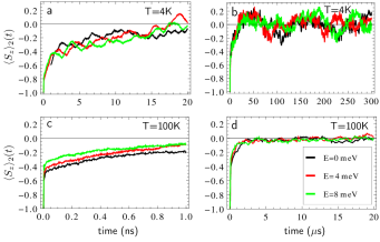
Figure 3: Return to equilibrium for $S_{z}$ of a single adatom spin coupled to 8 substrate electrons. The relaxation is shown for temperatures of $T=4$ K, $T=100$ K, different values of $E$ and fixed $D=1$ meV. Fig. 3 a) and 3 c): The short time behavior shows a faster relaxation for a higher temperature. Fig. 3 b) and 3 d): The long time behavior shows smaller quantum fluctuations around thermal equilibrium for higher temperatures. The different time scales on the $x$-axis should be noted.

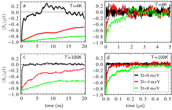
Figure 4: Return to equilibrium for $S_{z}$ and different values of $D$ of a single adatom spin coupled to 8 substrate electrons. The relaxation time grows with increasing value of the anisotropy barrier $D$. Fig. 4a) and 4c): The short time behavior shows a faster relaxation for a higher temperature. Fig. 4b) and 4d): The long time behavior shows smaller quantum fluctuations around thermal equilibrium for higher temperatures. The different time scales on the $x$-axis should be noted.

It can be seen that in all cases the fluctuations decrease with increasing temperature. Depending on the time scale, in all cases the evaluated function $\omega^{\beta P}(\tau_{t}(S_{z}))$ can be approximated by a function starting from $-1$ with an exponential decay to zero. Fluctuations induced by the temperature are not able to switch the spin back to $\langle S_{z}\rangle\approx-1$. A similar behavior has been found experimentally in LothIBM , where a single Fe spin was excited with a high voltage pump, corresponding to a strong perturbation in our model, and the relaxation process of this single spin was investigated. The magnetization showed the exponential decay for first time period, followed by small fluctuations near thermal equilibrium. The temperature was unable to switch the spin to its initial value for $t=0$. The appearance of larger fluctuations for a lower temperature might be explained by energy considerations. A system at a lower temperature has less energy than a system at a higher temperature. A perturbation $P$ corresponds to an additional amount of energy. Notice that for an infinite system this additional energy is negligible and an exact thermalization might take place Bratelli . The relative ratio between the energy of perturbation and the energy of the free system is larger at lower temperatures. This might be a reason for the stronger fluctuations at lower temperatures. Another important effect at low temperatures are ”quantum fluctuations”, which become extinct with increasing temperature. We can also see that for higher temperatures the quantum spin of the adatom returns faster to equilibrium, i.e. the adatom relaxation time becomes shorter. With increasing value of $D$ the relaxation time also increases. This is in agreement with the statement that a spin ”up” or ”down” state becomes more stable with increasing anisotropy barrier. For increasing $E$ (see Fig. 3 a,c) an inverted behavior has been observed for short times.

Now we will apply Eq. (6) and (8) to model the STM measurement process as a time average. As an example we take cobalt adatoms on platinum (111) Meier:Science(2008) . As described in the introduction the reason for zero magnetization of a Co adatom on Pt(111) at zero external field was still unclear (see Fig. 5). The Hamiltonian for the cobalt atom is given by Meier:Science(2008)

$$H=-mB_{z}S_{z}-KS^{2}_{z},$$ (15)

with $m=3.7$ $\mu_{B}$ and $K=9$ meV. From this Hamiltonian a nearly vanishing probability for the states $|-\frac{3}{2}\rangle$, $|-\frac{1}{2}\rangle$, $|\frac{1}{2}\rangle$ and $|\frac{3}{2}\rangle$ can be found in thermal equilibrium.

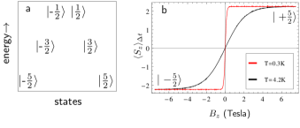
Figure 5: a) The high energy states $|-\frac{3}{2}\rangle$, $|-\frac{1}{2}\rangle$, $\mid\frac{1}{2}\rangle$ and $\mid\frac{3}{2}\rangle$ got a vanishing probability in thermal equilibrium. The preferred states are those where the spin points ”up” $\mid\frac{5}{2}\rangle$ or ”down” $\mid-\frac{5}{2}\rangle$. b) The time averaged magnetization curves for two different temperatures show agreement of Eq. (8) with the experimental data in Meier:Science(2008) . For high positive magnetic field mostly the $\mid\frac{5}{2}\rangle$ state is occupied and for high negative field it is the $\mid-\frac{5}{2}\rangle$ state.

If the spin has been prepared to be polarized in positive or negative $z$-direction it is not a priori clear how the spin can switch in the opposite state because of the high anisotropy barrier. The temperature of $T=0.3$ K and $T=4.2$ K used in this experiment is much too low to switch the spin over the anisotropy barrier of $K=9$ meV. The Néel-Brown law predicts a switching time of a few million years, which is in disagreement with the short resolution time of $10$ ms of the SP-STM technique used in Meier:Science(2008) . The absence of the transverse anisotropy term $E(S^{2}_{x}-S^{2}_{y})$ in the free system prevents direct transitions under the barrier between the $|\frac{5}{2}\rangle$ and $|-\frac{5}{2}\rangle$ states. To explain the zero expectation value of $S_{y}$ a quantum tunneling or a current induced magnetization switching mechanism has been speculatively proposed Meier:Science(2008) . Here, we check this proposition by numerical calculations.

The perturbation is taken to be $P=J\sum_{i}\vec{S}\vec{\sigma}_{i}+\sum_{i}\vec{m}_{\mathrm{tip}}\vec{\sigma}_{i}$, with the magnetization $\vec{m}_{\mathrm{tip}}$ of the tip and the Pauli matrices corresponding to the tunneling electrons. When the cobalt atom gets perturbed because of the interaction with the tunneling electrons it gets out of equilibrium and the question about the occupation probability of the states $|\frac{5}{2}\rangle$,…,$|-\frac{5}{2}\rangle$ arises. A related question is, in which way the spin gets from the $|\frac{5}{2}\rangle$ to the $|-\frac{5}{2}\rangle$ state. Especially interesting is the case of zero magnetic field where the SP-STM measurement provides a time averaged expectation value $\langle S_{z}\rangle_{\Delta T}=0$. Fig. 6 a), b) gives the time evolution $\omega^{\beta}(\tau^{P}_{t}(S_{z}))$ for the z-component of the magnetization, for two different values of external magnetic field $B_{z}$. In agreement with experimental data $\langle S_{z}\rangle_{\Delta t}=0$ for $B_{z}=0$, while it increases with increasing $B_{z}$.

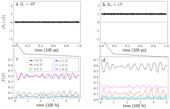
Figure 6: The time evolution of the adatom spin for the $z$-component as a function of time are shown for a), c) $B_{z}=0$ and b), d) $B_{z}=1$ Tesla. The expectation value fluctuates around thermal equilibrium at $T=4.2$ K. The occupation probabilities $P_{i}$ for the states $i=|\frac{5}{2}\rangle$,…,$|-\frac{5}{2}\rangle$ as a function of time are shown for c) $B_{z}=0$ and d) $B_{z}=1$ Tesla.

As it is seen in Fig.6 c) at $t=0$ the total signal is composed of the superposition of $|\frac{5}{2}\rangle$ and $|-\frac{5}{2}\rangle$. As the tunneling current is switched on the occupation probabilities of those states start to oscillate. The amplitude of oscillations increases with increasing parameter $J$ and also depends on $\vec{m}_{\mathrm{tip}}$. The appearance of fluctuations in the occupation probabilities means that not only $\mid\pm\frac{5}{2}\rangle$ states become occupied. In other words magnetization switching occurs. The results demonstrate that even a weak perturbation due to tunneling electrons initiates a quantum tunneling in otherwise diagonal systems. The expectation value of magnetization at $B_{z}=0$ remains nearly zero.

IV Conclusion

The non-equilibrium dynamics of adatoms on different substrates under the action of a magnetic STM tip has been studied. A satisfactory agreement of Eq. (7) and (6) with experimental data has been found, when the perturbation has been identified as the interaction between the STM-tip and the sample. It has been shown that the application of a perturbed KMS state in (7) is well suited to model relaxation dynamics of magnetic atoms at finite temperature. The application of the perturbed dynamics in Eq. (6) can be used to investigate the system dynamics during an SP-STM measurement.

Fig. 2, 3 and 4 demonstrate that thermalization can be achieved for relatively small systems, which can be calculated using exact diagonalization. The relaxation can be approximated with an exponential function, which is in agreement with experimental results. It is demonstrated that the lifetime of single adatoms increases with increasing anisotropy barrier and decreasing temperature.

We were able to reproduce the experimentally obtained time averages of expectation values. Additionally the dynamics of the sample (see Fig. 6) for time scales which are shorter than the resolution time of the STM has been described using the integrand of Eq. (8).

A finer mathematical structure Bratelli can be implemented into the rough structure described in section II. This is done by the replacement of the substitution of the Hamiltonians $H\rightleftarrows H+P$ by $C^{*}$-dynamical systems $(\mathcal{A},\tau)\rightleftarrows(\mathcal{A},\tau^{P})$. This general mathematical structure can also be applied to fermionic lattice systems, e.g. the Hubbard model, and continuous fermionic systems in the algebraic approach to Quantum Field Theory.

- (1) R. Wiesendanger et al, Observation of Vacuum Tunneling of Spin-Polarized Electrons with the Scanning Tunneling Microscope, PRL Vol. 65, Nu.2, 9 July (1990)
- (2) R. Wiesendanger, Rev. Mod. Phys. 81, 1495 (2009).
- (3) F. Meier et al., Science 320, 82 (2008).
- (4) A. A. Khajetoorians et al., Nature 467, 1084 (2010).
- (5) O. Bratelli and D. W. Robinson, Operator Algebras and Quantum Statistical Mechanics II (Springer Verlag, Berlin, 1981).
- (6) H. Araki and E. Barouch, J. Statist. Phys., 31, 2 (1983).
- (7) H. Araki, Publ.RIMS, Kyoto Univ. 20, 277-296 (1984).
- (8) B. Nachtergaele et al., J. Stat. Phys., 124, 1–13 (2006).
- (9) B. Nachtergaele and R. Sims, Markov Processes Rel. Fields, 13, 315–329 (2007).
- (10) E. Hazma, S. Michalakis, B. Nachtergaele and R. Sims, Approximating the Ground State of gapped Quantum Spin Systems, J. Math. Phys. 50, 095213 (2009).
- (11) B. Nachtergaele, Quantum Spin Systems, arXiv:math-ph/0409006v1
- (12) B. Nachtergaele and R. Sims, Recent Progress in Quantum Spin Systems, Markov Processes Relat. Fields 13, 315-329 (2007).
- (13) B. Nachtergaele, Y. Ogota and R. Sims, Propagation of Correlations in Quantum Lattice Systems, J. Stat. Phys. 124, 1–13 (2006).
- (14) T. Michoel, B. Nachtergaele and W. Spitzer, Transport of interface states in the Heisenberg chain, J. Phys. 49, A 41 (2008).
- (15) M. Balzer and M. Potthoff, Non-equilibrium cluster-perturbation theory, Phys. Rev. B 83, 195132 (2011).
- (16) M. Balzer, N. Gdaniec and M. Potthoff, Krylov-space approach to the equilibrium and the nonequilibrium single-particle Green’s function, J. Phys.: Condens. Matter 24 035603 (2012).
- (17) K. R. Patton, S. Kettemann, A. Zhuravlev and A. Lichtenstein, Spin-polarized tunneling microscopy and the Kondo effect, Phys. Rev. B 76, 100408(R) (2007).
- (18) E. Gull, A. Millis, A. Lichtenstein, A. Rubtsov, M. Troyer and P. Werner, Continuous-time Monte Carlo methods for quantum impurity models, Rev. Mod. Phys. 83, 349–404 (2011).
- (19) T. Stapelfeldt et al, Domain Wall Manipulation with a Magnetic Tip, Phys. Rev. Lett. 107, 027203.
- (20) D. W. Robinson, Statistical Mechanics of Quantum Spin Systems, Commun. math. Phys. 6, 151-160 (1967).
- (21) D. W. Robinson, Statistical Mechanics of Quantum Spin Systems II, Commun. math. Phys. 7, 337-348 (1968).
- (22) D. W. Robinson, Statistical Mechanics of Quantum Spin Systems III, Commun. math. Phys. 9, 327-338 (1968).
- (23) E. H. Lieb, The Classical Limit of Quantum Spin Systems, Commun. math. Phys. 31, 327-340 (1973).
- (24) E. H. Lieb and D. W. Robinson, The Finite Group Velocity of Quantum Spin Systems, Commun. math. Phys. 28, 251-257 (1972)
- (25) M. Keyl, T. Matsui, D. Schlingemann and R. F. Werner, On Haag Duality for Pure States of Quantum Spin Chain, R. Math. Physics, 20, Issue 06, pp. 707-724 (2008).
- (26) V. Jaksic and C.-A. Pillet, Mathematical Theory of Non-Equilibrium Quantum Statistical Mechanics, Journal of Statistical Physics, Vol. 108, Nos 5/6, (2002).
- (27) Y. Ogata, The Stability of the Non-Equilibrium Steady States, Commun. math. Phys. 245, 3 577-609 (2004).
- (28) A. A. Khajetoorians et al., PRL 106, 037205 (2011).
- (29) S. Loth et al., Science 329, 5999 (2010).