Three-dimensional coherence matrix and degree of polarization

Abstract

Inspecting three-dimensional partially polarized light fields we show that there is no unambiguous correspondence between the three-dimensional field and coherence matrix (or light beam tensor). Therefore, it is needed to clarify the definition of unpolarized light. We believe that unpolarized field should be treated as light of equiprobable polarizations similar to the case of two-dimensional light. Then degree of polarization bridges two definitions of the three-dimensional degrees of polarization known in literature. We reveal that only 6 Stokes parameters are sufficient to describe the coherence matrix. All these parameters can be retrieved from the in-plane measurements of two-dimensional coherence matrices.

I Introduction

The well-established concept of polarization plays important part in the modern theories and applications. Optics of metamaterials, transformation optics, and nonlinear optics are the basis for constructing smart devices for effective light control. Together with the materials the electromagnetic fields become also more intricate. For example, accelerated Airy beams, nonparaxial Bessel beams, and knotted fields propose the novel interesting physics behind them Siviloglou ; Chen ; Novitsky ; Sukhov ; Irvine . With more complicated three-dimensional electromagnetic beams, the generalizationsMilione of the degree of polarization and coherence matrix may be appreciated.

The theory of polarization optics was developed in the aforetime centuries: Poincare’s sphere,Poincare Stokes parameters, Stokes Wolf’s coherence matrix,Wolf $2\times 2$ Jones matrix, Jones $4\times 4$ Mueller matrix, Mueller etc. The coherence matrix serves for the description of a partially polarized beam, when it propagates in a certain direction. In Refs. Fedorov65 ; Fedorov the coherence matrix was generalized to the so called light beam tensor, which keeps invariant with respect to the rotations in the three-dimensional space. The coherence matrix is the special representation of this tensorial quantity.

In the present paper we investigate the light beam tensor for the three-dimensional electromagnetic beams. In the previous studies, the three-dimensional coherence matrix, 9 Stokes parameters, and three-dimensional degree of polarization were introduced.Setala2002 ; Setala2009 However, the proposed degree of polarization is just the mathematical generalization of the two-dimensional coherence matrix. Physically justified 3D degree of polarization Ellis ; EllisOC05 ; EllisOL04 ; Brosseau ; Refregier as the ratio of the intensity of the fully polarized field to the total intensity turns out to be different quantity.

In Section II of the paper we discuss the definition of the unpolarized field and find out that the 3D coherence matrix is not able to describe the general beam structure. In Section III we derive that the mathematically generalized degree of polarization Setala2002 ; Setala2009 coincides with physically defined one Ellis when the beam consists of completely polarized and completely unpolarized components Aunon . In this case we study the light beam tensor in details. This beam tensor involves only 6 independent parameters, therefore, requires 6 Stokes parameters. In Section IV, the choice of the 6 Stokes parameters is discussed. The problem of the reconstruction of the three-dimensional light beam’s tensor using the in-plane measurements is considered in Section V. Section VI concludes the paper.

II Unpolarized light

When one characterizes 2D partially polarized light, it is intuitively clear that the polarized light is the coherent superposition of partial waves, while unpolarized light is non-coherent superposition of partial waves which polarizations are equiprobable. For the 3D light one naturally keeps the definition of polarized wave EllisOL04 . Unpolarized light is not well defined and treated as something complicated. In this Section we justify the definition of the 3D unpolarized light as superposition of equiprobably polarized non-coherent waves in the three-dimensional space.

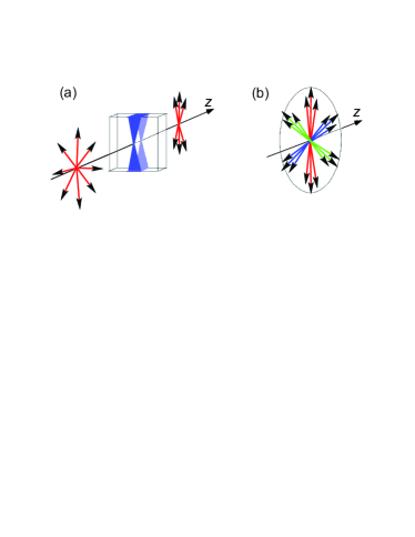
Figure 1: (a) Incident natural light is polarized within the angle sector in the beam plane. (b) 2D beam generated as the superposition of beams unpolarized in three angle sectors.

Let us start with the 2D unpolarized light. Is it really clear that the partially polarized beam consists of completely polarized beam and completely unpolarized beam and, therefore, can be described by the 2D coherence matrix? Consider a device (incomplete polarizer) that can transmit only the waves which polarizations belong to an angle sector as indicated in Fig. 1(a). Then the incident naturally polarized beam becomes unpolarized light which polarizations are equiprobable in this angle sector. When several such beams are mixed (Fig. 1(b)), the 2D state of polarization cannot be fully described by the regular coherence matrix. Should we say that the coherence matrix of the 2D field is limited? We think it is just needed to consider usual definition of the unpolarized light as superposition of equiprobable polarizations.

The similar story is usually narrated for 3D electromagnetic fields. It is accepted that a 3D partially polarized field can be presented as superposition of completely polarized light, completely unpolarized light (mix of equiprobably polarized waves), and something else which is related to unpolarized light (2D unpolarized light according to Ref. EllisOC05 ). In general, electric field of the 3D unpolarized light can be treated as the sum of electric fields of different unpolarized electromagnetic beams, such as in-plane completely unpolarized, completely unpolarized waves with wavevectors lying on the cone (Bessel beams), etc. Some examples are demonstrated in Fig. 2. It is evident that if the 3D unpolarized field is formed by many such partial beams, we need much more than 9 parameters which are introduced to describe the $3\times 3$ coherence matrix. Thus we fundamentally cannot retrieve the realistic structure of the 3D field, if we know nothing of the field.

Let us inspect the consequences of the above reasoning applied for the coherence matrices (light beam tensors). Superposition of non-coherent elementary plane waves ${\bf E}^{(s)}$ with the same direction of propagation ${\bf k}^{(s)}=k{\bf n}$, where $s$ enumerates the elementary waves, ${\bf k}^{(s)}$ is the wavevector, $|{\bf n}|=1$, is described by the light beam tensor Fedorov65 ; Fedorov

$$\Phi_{2}=\sum_{s}{\bf E}^{(s)}\otimes{\bf E}^{(s)\ast},\qquad\Phi_{2}{\bf n}={\bf n}\Phi_{2}=0,$$ (1)

where ${\bf a}\otimes{\bf b}$ is the dyad (tensor product of the vectors ${\bf a}$ and ${\bf b}$). In the index form, $({\bf a}\otimes{\bf b})_{ij}=a_{i}b_{j}$, $i,j=1,2,3$. Quantity $\Phi_{2}$ defined by Eq. (1) is indeed tensor, since it is composed of elementary tensors, dyads.

Three-dimensional light represents the superposition of elementary waves, which can possess not only random phases and polarizations, but also directions of propagation, i.e. ${\bf k}^{(s)}=k^{(s)}{\bf n}^{(s)}$. Thus, the light beam tensor equals

$$\Phi=\Phi_{3}=\sum_{s}{\bf E}^{(s)}\otimes{\bf E}^{(s)\ast}.$$ (2)

In contrast to Eq. (1), the additional limitations on the beam tensor $\Phi{\bf n}={\bf n}\Phi=0$ are not valid anymore.

When the beam consists of coherent elementary waves, it is fully polarized and the beam’s tensor $\Phi={\bf E}\otimes{\bf E}^{\ast}$. In the opposite situation of 3D fully unpolarized light with equiprobable polarizations the beam tensor does not have a preferred direction and, therefore, $\Phi=A\textbf{1}$, where ${\bf 1}$ is the identity tensor in the three-dimensional space and $A$ is a coefficient.

As any self-conjugated tensor ($\Phi^{\dagger}=\Phi$, here ${\dagger}$ denotes Hermitian conjugate), three-dimensional beam’s tensor can be presented as a spectral expansion of the form

$$\Phi=\lambda_{1}{\bf u}_{1}\otimes{\bf u}_{1}^{\ast}+\lambda_{2}{\bf u}_{2}\otimes{\bf u}_{2}^{\ast}+\lambda_{3}{\bf u}_{3}\otimes{\bf u}_{3}^{\ast},$$ (3)

where $\lambda_{i}=\lambda_{i}^{\ast}$ and ${\bf u}_{i}$ ($i=1,2,3$) are the eigenvalues and eigenvectors of $\Phi$, respectively. The eigenvectors are orthogonal and normalized as ${\bf u}_{i}{\bf u}^{\ast}_{j}=\delta_{ij}$, where $\delta_{ij}$ is Kronecker’s delta. Spectral decomposition for the identity tensor reduces to the completeness condition ${\bf 1}={\bf u}_{1}\otimes{\bf u}_{1}^{\ast}+{\bf u}_{2}\otimes{\bf u}_{2}^{\ast}+{\bf u}_{3}\otimes{\bf u}_{3}^{\ast}$. Tensor $\Phi$ can be described by 9 independent parameters.

On the other hand, the general definition (2) can be written in the form different from Eq. (3), if we know something of the electromagnetic beam. For example, let the 3D field includes the superposition of 2D completely unpolarized beams with directions defined by the unit vectors ${\bf n}_{\alpha}$ ($\alpha=1,\ldots,M$). Then the beam tensor reads

$$\Phi={\bf E}_{p}\otimes{\bf E}_{p}^{\ast}+A{\bf 1}+\sum_{\alpha=1}^{M}B_{\alpha}I_{\alpha},$$ (4)

where $I_{\alpha}={\bf 1}-{\bf n}_{\alpha}\otimes{\bf n}_{\alpha}$ is the projector onto the plane with normal vector ${\bf n}_{\alpha}$. If the directions of the normal vectors are known, the tensor Eq. (4) depends on 5 parameters of polarized field (${\bf E}_{p}\otimes{\bf E}_{p}^{\ast}$), 1 parameter of 3D fully unpolarized beam ($A{\bf 1}$), and $M$ parameters of 2D unpolarized beams ($\sum_{\alpha=1}^{M}B_{\alpha}I_{\alpha}$). If $6+M>9$, we cannot reconstruct the structure of the beam using 9 parameters of the general 3D coherence matrix Eq. (3). Nevertheless, the beam parameters can be found, if we make more measurements than 9. But this can be done only if we know the form of the coherence matrix, e.g. Eq. (4).

If the directions of propagation of the 2D unpolarized beams are unknown, it is necessary to introduce two additional parameters for each real unit vector ${\bf n}_{\alpha}$, i.e. the number of unknown parameters is equal to $6+3M$. When $M=1$, the coherence matrix indeed can be presented as the sum of coherent part, completely 3D unpolarized part, and completely 2D unpolarized part, respectively:

$$\Phi={\bf E}_{p}\otimes{\bf E}_{p}^{\ast}+A{\bf 1}+B({\bf 1}-{\bf n}\otimes{\bf n}).$$ (5)

If the directions of propagation of 2D unpolarized beams are known, it is feasible to specify 3D field using the coherence matrix Eq. (4) for $M\leq 3$.

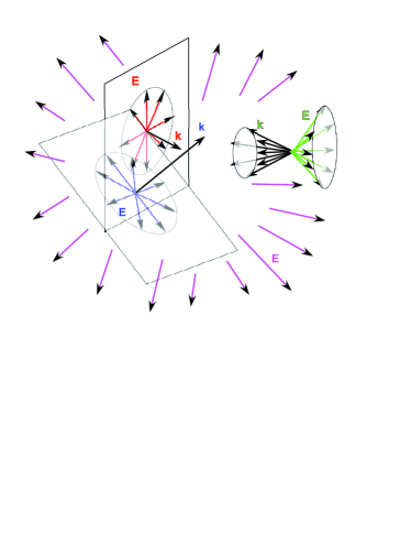
Figure 2: 3D partly polarized field as superposition of 3D unpolarized beam (electric fields are equiprobably directed), two in-plane unpolarized beams, and on-cone unpolarized beam. Black arrows indicate wavevectors ${\bf k}$, colored arrows show electric fields ${\bf E}$.

Concluding this section, it is not possible to determine the actual structure of either 3D or 2D field, if we know nothing about the field itself, because the coherence matrix does not carry sufficient information. In 2D case, it is accepted that the fully unpolarized light possesses equiprobable in-plane polarizations. We are convinced that the similar definition of the completely unpolarized light should be used for the 3D light. If the beam is arbitrary, it is not sufficient to set even 9 components of the coherence matrix (3) to unambiguously determine the structure of the beam.

III Three-dimensional light

III.1 Form of light beam’s tensor

According to the results of the previous Section we consider the 3D field as composed of completely 3D polarized light and completely 3D unpolarized light. This means that there are no specific directions and two forms of light beam tensor

$$\Phi=(\lambda_{1}-\lambda_{3}){\bf u}_{1}\otimes{\bf u}_{1}^{\ast}+(\lambda_{2}-\lambda_{3}){\bf u}_{2}\otimes{\bf u}_{2}^{\ast}+\lambda_{3}{\bf 1}$$ (6)

and

$$\Phi=(\lambda_{1}-\lambda_{2}){\bf u}_{1}\otimes{\bf u}_{1}^{\ast}+(\lambda_{3}-\lambda_{2}){\bf u}_{3}\otimes{\bf u}_{3}^{\ast}+\lambda_{2}{\bf 1}$$ (7)

should be equivalent. Thus we conclude that $\lambda_{2}=\lambda_{3}$ and the beam tensor of the three-dimensional light equals

$$\Phi=(\lambda_{1}-\lambda_{2}){\bf u}_{1}\otimes{\bf u}_{1}^{\ast}+\lambda_{2}{\bf 1},$$ (8)

where $\Phi_{p}=(\lambda_{1}-\lambda_{2}){\bf u}_{1}\otimes{\bf u}_{1}^{\ast}$ and $\Phi_{u}=\lambda_{2}{\bf 1}$ describe completely polarized and unpolarized light, respectively.

3D field is completely polarized, when eigenvalue $\lambda_{2}=0$, and completely unpolarized, when $\lambda_{1}=\lambda_{2}$. For all other values $0\leq\lambda_{2}\leq\lambda_{1}$ one gets partially polarized light. Eq. (8) has clear physical meaning, because it includes intuitively defined polarized and unpolarized beam’s tensors. The form of the three-dimensional beam tensor (8) can be formulated using another argumentation. In the three-dimensional space, there is the single distinguished direction of the polarized electric field ${\bf u}_{1}$. Therefore, we can construct only the tensor of the form $\alpha{\bf u}_{1}\otimes{\bf u}_{1}^{\ast}+\beta{\bf 1}$.

Two-dimensional light beam tensor is characterized by two distinguished directions, ${\bf u}_{1}$ and ${\bf n}$, and can be presented in the similar form as Fedorov65 ; Fedorov

$$\Phi_{2}=(\lambda_{1}-\lambda_{2}){\bf u}_{1}\otimes{\bf u}_{1}^{\ast}+\lambda_{2}I,$$ (9)

where $I={\bf 1}-{\bf n}\otimes{\bf n}$ is the projection operator onto the plane with normal vector ${\bf n}$ and ${\bf u}_{1}=I{\bf u}_{1}$ is the vector in the plane orthogonal to ${\bf n}$. Eq. (8) differs from Eq. (9) with the three-dimensional vector ${\bf u}_{1}$ and three-dimensional identity tensor.

III.2 Degree of polarization

Eq. (8) provides intuitive definition of the three-dimensional degree of polarization in terms of the eigenvalues of the beam tensor. The trace of the coherence matrix ${\rm Tr}(\Phi)$ is proportional to the intensity of light. Intensity of the polarized and unpolarized beams are ${\rm Tr}(\Phi_{p})=(\lambda_{1}-\lambda_{2})$ and ${\rm Tr}(\Phi_{u})=3\lambda_{2}$, respectively. Degree of polarization for the three-dimensional light is equal to

$$P_{3}=\frac{{\rm Tr}(\Phi_{p})}{{\rm Tr}(\Phi_{p})+{\rm Tr}(\Phi_{u})}=\frac{\lambda_{1}-\lambda_{2}}{\lambda_{1}+2\lambda_{2}},$$ (10)

The two eigenvalues of the coherence matrix can be found using the two invariants of $\Phi$. Usually the trace of the matrix ${\rm Tr}(\Phi)\equiv(\Phi)_{t}$ and the trace of the squared matrix ${\rm Tr}(\Phi^{2})\equiv(\Phi^{2})_{t}$ are used. From $\Phi=\lambda_{1}{\bf u}_{1}\otimes{\bf u}_{1}^{\ast}+\lambda_{2}({\bf u}_{2}\otimes{\bf u}_{2}^{\ast}+{\bf u}_{3}\otimes{\bf u}_{3}^{\ast})$ one easily derives

$$(\Phi)_{t}=\lambda_{1}+2\lambda_{2},\qquad(\Phi^{2})_{t}=\lambda^{2}_{1}+2\lambda^{2}_{2}.$$ (11)

For $\lambda_{2}\leq\lambda_{1}$ we obtain

$$\lambda_{1}=\frac{1}{3}\left((\Phi)_{t}+\sqrt{6(\Phi^{2})_{t}-2(\Phi)_{t}^{2}}\right),$$

$$\lambda_{2}=\frac{1}{6}\left(2(\Phi)_{t}-\sqrt{6(\Phi^{2})_{t}-2(\Phi)_{t}^{2}}\right).$$ (12)

Degree of polarization takes the form

$$P_{3}=\sqrt{\frac{3}{2}\frac{(\Phi^{2})_{t}}{(\Phi)_{t}^{2}}-\frac{1}{2}}.$$ (13)

For completely polarized light $P_{3}=1$ and $(\Phi^{2})_{t}=(\Phi)_{t}^{2}$. Completely unpolarized light is characterized by $P_{3}=0$ and $(\Phi^{2})_{t}=(\Phi)_{t}^{2}/3$. Thus, the degree of polarization is in the interval $0\leq P_{3}\leq 1$.

It should be noted that the generalized degree of polarization obtained in Ref. Setala2002 coincides with Eq. (13). This means that the generalization of the 2D degree of polarization inherits the property of partially polarized beam to be split into completely polarized and unpolarized parts. In other words, the degree of polarization in Ref. Setala2002 corresponds to the restricted coherence matrix Eq. (8). When the coherence matrix is the general $3\times 3$ Hermitian matrix, the degree of polarization is expressed as $(\lambda_{1}-\lambda_{2})/(\lambda_{1}+\lambda_{2}+\lambda_{3})$ (see Ref. Ellis ). In this case, the three eigenvalues can be found using three invariants of the coherence matrix ${\rm Tr}(\Phi)$, ${\rm Tr}(\Phi^{2})$, and ${\rm det}(\Phi)$, and closed-form expression for $P_{3}$ is expected to be more complicated. For the derived beam tensor (8) the generalized and physically justified degrees of polarization are agreed as it has been pointed out in Ref.Aunon

III.3 From 3D to 2D degree of polarization

Transition from the three-dimensional light to the two-dimensional one can be performed by excluding one eigenvector (assuming, e.g., ${\bf u}_{3}=0$). In the previously derived formulae we have considered vector ${\bf u}_{3}$ normalized by unity, what should be violated in the 2D case. So, we will explicitly write the vector ${\bf u}_{3}$ in equations. Then ${\rm Tr}(\Phi_{p})=(\lambda_{1}-\lambda_{2})$ and ${\rm Tr}(\Phi_{u})=\lambda_{2}(2+|{\bf u}_{3}|^{2})$, and

$$P_{3}=\frac{\lambda_{1}-\lambda_{2}}{\lambda_{1}+\lambda_{2}(1+|{\bf u}_{3}|^{2})}.$$ (14)

In terms of the invariants of the coherence matrix, the degree of polarization of the beam takes the form

$$P_{3}=\alpha_{0}+\sqrt{\alpha_{1}\frac{(\Phi^{2})_{t}}{(\Phi)_{t}^{2}}-\alpha_{2}},$$ (15)

where

$$\alpha_{0} = \frac{|{\bf u}_{3}|^{2}(|{\bf u}_{3}|^{2}-1)}{2(1+|{\bf u}_{3}|^{2}+|{\bf u}_{3}|^{4})},\qquad\alpha_{1}=\frac{(2+|{\bf u}_{3}|^{2})^{2}}{2(1+|{\bf u}_{3}|^{2}+|{\bf u}_{3}|^{4})},$$

$$\alpha_{2} = \frac{(2+|{\bf u}_{3}|^{2})^{2}(1+|{\bf u}_{3}|^{4})}{4(1+|{\bf u}_{3}|^{2}+|{\bf u}_{3}|^{4})^{2}}.$$ (16)

Eqs. (14) and (15) are valid both for three-dimensional and two-dimensional fields. For 3D and 2D fields one needs to apply $|{\bf u}_{3}|^{2}=1$ and $|{\bf u}_{3}|^{2}=0$, respectively.

III.4 From 3D to 2D light beam’s tensor

Three-dimensional beam’s tensor (2) is the sum of the dyads ${\bf E}^{(s)}\otimes{\bf E}^{(s)\ast}$. When we want to study the light on a plane, we need to consider projected fields $I_{\bf m}{\bf E}^{(s)}$, where $I_{\bf m}={\bf 1}-{\bf m}\otimes{\bf m}$ is the projector onto the plane with normal vector ${\bf m}$ ($|{\bf m}|=1$). The beam tensor composed of such projected electric fields equals

$$\Phi_{2}({\bf m})=\sum_{s}I_{\bf m}{\bf E}^{(s)}\otimes I_{\bf m}{\bf E}^{(s)\ast}=I_{\bf m}\Phi I_{\bf m}.$$ (17)

When the elementary waves of the beam propagate in the same direction ${\bf n}$, we obtain the ordinary two-dimensional coherence matrix

$$\Phi_{2}=I_{\bf n}\Phi I_{\bf n}=(\lambda_{1}-\lambda_{2}){\bf u}_{1}\otimes{\bf u}_{1}^{\ast}+\lambda_{2}I_{\bf n}.$$ (18)

Here $I_{\bf n}{\bf u}_{1}={\bf u}_{1}$ is the electric field vector in the plane of constant phase. It should be noted that in general we can write the beam tensor projection on any plane according to Eq. (17).

IV Stokes parameters

If $\Phi$ was the general matrix (3), it would contain 9 independent parameters, which could be written as Stokes parameters for the three-dimensional fields. However, the coherence matrix has reduced form (8), which decreases the number of independent parameters.

Let us calculate the number of independent parameters of beam’s tensor (8). Normalized complex vector ${\bf u}_{1}$ can be expressed in terms of 4 real quantities, $a$, $b$, $\varphi_{1}$, and $\varphi_{2}$, as

$${\bf u}_{1}=a{\bf e}_{x}+b{\rm e}^{i\varphi_{1}}{\bf e}_{y}+\sqrt{1-a^{2}-b^{2}}{\rm e}^{i\varphi_{2}}{\bf e}_{z}.$$ (19)

(Coefficient in front of ${\bf e}_{x}$ can be regarded as real, because ${\bf u}_{1}$ enters beam’s tensor as ${\bf u}_{1}\otimes{\bf u}_{1}^{\ast}$.) Adding two more real eigenvalues $\lambda_{1}$ and $\lambda_{2}$, we claim 6 independent parameters for the light beam tensor.

Definition of the three-dimensional beam tensor in the form (8) does not take into account the transversality condition $\nabla{\bf E}=0$. Completely polarized electric field ${\bf E}$ can be found from the definition $\Phi_{p}={\bf E}\otimes{\bf E}^{\ast}=(\lambda_{1}-\lambda_{2}){\bf u}_{1}\otimes{\bf u}_{1}^{\ast}$. Then the electric field equals ${\bf E}=\exp(i\psi)\sqrt{\lambda_{1}-\lambda_{2}}{\bf u}_{1}$, while the transversality condition reads

$$\nabla({\rm e}^{i\psi}\sqrt{\lambda_{1}-\lambda_{2}}{\bf u}_{1})=0.$$ (20)

In general, the phase $\psi({\bf r})$ distribution cannot be supposed and Eq. (20) is the differential equation for the phase $\psi$:

$$i\sqrt{\lambda_{1}-\lambda_{2}}({\bf u}_{1}\nabla\psi)+\nabla(\sqrt{\lambda_{1}-\lambda_{2}}{\bf u}_{1})=0.$$ (21)

The number of independent parameters for $\Phi$ is still 6.

When we know the phase, e.g., $\psi=\beta z$ ($\beta$ is the propagation constant of the beam), the transversality condition

$$-\beta\sqrt{\lambda_{1}-\lambda_{2}}({\bf e}_{z}{\bf u}_{1})+\nabla(\sqrt{\lambda_{1}-\lambda_{2}}{\bf u}_{1})=0$$ (22)

becomes the pair of restrictions on $\lambda_{1,2}$ and ${\bf u}_{1}$ of the form ${\rm Re}(\nabla{\bf E})=0$ and ${\rm Im}(\nabla{\bf E})=0$, so that the beam is fully described by the 4 independent parameters (Stokes parameters). When the beam consists of the plane waves propagating in the direction of vector ${\bf n}$, $\psi({\bf r})=k({\bf n}{\bf r})$ and $\sqrt{\lambda_{1}-\lambda_{2}}{\bf u}_{1}$ is constant. Eq. (22) reads ${\bf n}{\bf u}_{1}=0$ or ${\bf n}{\bf E}=0$. This is equivalent to the conditions $\Phi_{2}{\bf n}={\bf n}\Phi_{2}=0$ on the coherence matrix used in the definition (1).

Thus, if there are no preferred directions, the transversality condition just exhibits the differential equation for the phase $\psi$ and does not decrease the number of the independent parameters $a$, $b$, $\varphi_{1}$, $\varphi_{2}$, $\lambda_{1}$, and $\lambda_{2}$. If the phase $\psi$ is somehow defined, there are two additional equations for the parameters, and we can use only $a$, $\varphi_{1}$, $\lambda_{1}$, and $\lambda_{2}$. So, we should have 6 Stokes parameters for truly three-dimensional fields and 4 Stokes parameters for 2D fields, when we can introduce the preferred direction (say, the direction of the beam propagation).

The Stokes parameters can be introduced as it was done in Ref. Setala2002 but then we need to choose only 6 parameters of 9, which are independent. The rest 3 parameters can be expressed using the independent 6 parameters. One of such links between the Stokes parameters is shown below:

$$\frac{\Lambda_{1}^{2}+\Lambda_{2}^{2}}{\Lambda_{3}^{2}}\left[\frac{\Lambda_{4}^{2}+\Lambda_{5}^{2}}{\Lambda_{6}^{2}+\Lambda_{7}^{2}}-1\right]^{2}=4\frac{\Lambda_{4}^{2}+\Lambda_{5}^{2}}{\Lambda_{6}^{2}+\Lambda_{7}^{2}},$$ (23)

where $\Lambda_{j}$ ($j=0,\ldots,8$) are the Stokes parameters introduced in Ref. Setala2002 for the three-dimensional fields. Two more links can be derived.

However, since most of the Stokes parameters $\Lambda_{j}$ have no physical sense and can be found from the coherence matrix, we propose another set of the Stokes parameters. For example, it is more convenient to use 4 conventional Stokes parameters in some plane (e.g., in ($x$, $y$) plane) and two more parameters in another plane (e.g., in ($x$, $z$) plane):

$$S_{0} = \Phi_{xx}+\Phi_{yy},\qquad S_{1}=\Phi_{xx}-\Phi_{yy},$$

$$S_{2} = \Phi_{xy}+\Phi_{yx},\qquad S_{3}=i(\Phi_{yx}-\Phi_{xy}),$$

$$S_{4} = \Phi_{xz}+\Phi_{zx},\qquad S_{5}=i(\Phi_{zx}-\Phi_{xz}).$$ (24)

Then $S_{0}$ is proportional to the field intensity in the plane of detector and $S_{3}$ is proportional to the spin angular momentum in the $z$-direction.

From the point of view of physics the field intensities and spin angular momenta are beneficial as independent parameters. Therefore, we also propose the physical Stokes parameters for the three-dimensional beams:

$$S^{\prime}_{0} = S_{0}=\Phi_{xx}+\Phi_{yy},\qquad S^{\prime}_{1}=\Phi_{xx}+\Phi_{zz},$$

$$S^{\prime}_{2} = \Phi_{yy}+\Phi_{zz},\qquad S^{\prime}_{3}=S_{3}=i(\Phi_{yx}-\Phi_{xy}),$$

$$S^{\prime}_{4} = i(\Phi_{zx}-\Phi_{xz}),\qquad S^{\prime}_{5}=i(\Phi_{zy}-\Phi_{yz}).$$ (25)

Parameters $S^{\prime}_{0}$, $S^{\prime}_{1}$, and $S^{\prime}_{2}$ stand for the intensities in the planes ($x$, $y$), ($x$, $z$), and ($y$, $z$), respectively, while $S^{\prime}_{3}$, $S^{\prime}_{4}$, and $S^{\prime}_{5}$ describe the spin angular momenta in directions $z$, $y$, and $x$. $S^{\prime}_{0}$ and $S^{\prime}_{3}$ coincide with analogous quantities of the usual set of Stokes parameters $S_{j}$ ($j=0,1,2,3$). With the eigenvalues $\lambda_{1,2}$ and 4 parameters of the vector ${\bf u}_{1}$ (see Eq. (19)), the physical Stokes parameters take the form

$$S^{\prime}_{0} = \lambda_{p}(a^{2}+b^{2})+\lambda_{2},\quad S^{\prime}_{1}=\lambda_{p}(a^{2}+c^{2})+\lambda_{2},$$

$$S^{\prime}_{2} = \lambda_{p}(b^{2}+c^{2})+\lambda_{2},\quad S^{\prime}_{3}=-2\lambda_{p}ab\sin(\varphi_{1}),$$

$$S^{\prime}_{4} = -2\lambda_{p}ac\sin(\varphi_{2}),\quad S^{\prime}_{5}=-2\lambda_{p}bc\sin(\varphi_{2}-\varphi_{1}),$$ (26)

where $\lambda_{p}=\lambda_{1}-\lambda_{2}$ and $c=\sqrt{1-a^{2}-b^{2}}$. The two-dimensional Stokes parameters require $c=0$ or $a^{2}+b^{2}=1$. In this case we have only 4 independent parameters $\lambda_{1,2}$, $a$, and $\varphi_{1}$, and the physical Stokes parameters

$$S^{\prime}_{0} = \lambda_{p}+\lambda_{2},\quad S^{\prime}_{1}=\lambda_{p}a^{2}+\lambda_{2},$$

$$S^{\prime}_{2} = \lambda_{p}(1-a^{2})+\lambda_{2},\quad S^{\prime}_{3}=-2\lambda_{p}ab\sin(\varphi_{1}),$$

$$S^{\prime}_{4} = 0,\quad S^{\prime}_{5}=0$$ (27)

are reduced to the four quantities, which can be connected with the ordinary Stokes parameters as

$$S_{0} = S^{\prime}_{0},\qquad S_{1}=S^{\prime}_{1}-S^{\prime}_{2},$$

$$S_{2} = \sqrt{4(S^{\prime}_{0}-S^{\prime}_{1})(S^{\prime}_{0}-S^{\prime}_{2})-S_{3}^{\prime 2}},\qquad S_{3}=S^{\prime}_{3}.$$ (28)

V Reconstruction of 3D coherence matrix

Measurement of nine components of the coherence matrix for 3D fields were discussed in Ref. EllisPRL05 . Here we deal with the measurement of the components of the coherence matrix Eq. (8) using the measurement of the fields in the detector plane. Let us denote the normal vector to the detector plane as ${\bf m}$ and reveal how the position of this plane influences the beam’s tensor and degree of polarization.

V.1 Projected 3D beam’s tensor

We will determine characteristics of the 2D beam tensor as projection of the 3D beam tensor. The absolute value of the three-dimensional vector ${\bf u}_{1}$ projected on a plane is less than unity and we lose the information about vector component orthogonal to the detector ${\bf m}{\bf u}_{1}$. Then projected beam’s tensor

$$\Psi_{2}=I_{\bf m}\Phi_{3}I_{\bf m}=(\lambda_{1}-\lambda_{2})(I_{\bf m}{\bf u}_{1})\otimes(I_{\bf m}{\bf u}_{1}^{\ast})+\lambda_{2}I_{\bf m}$$ (29)

can be rewritten in the form

$$\Psi_{2}=(\lambda_{1}-\lambda_{2})|I_{\bf m}{\bf u}_{1}|^{2}{\bf v}\otimes{\bf v}^{\ast}+\lambda_{2}I_{\bf m},$$ (30)

where ${\bf v}=(I_{\bf m}{\bf u}_{1})/|I_{\bf m}{\bf u}_{1}|$ is situated in the plane with the normal vector ${\bf m}$, $|{\bf v}|=1$, and $I_{\bf m}$ is the projection operator. The detector-measured intensities of the completely polarized and unpolarized parts of the beam are $(\lambda_{1}-\lambda_{2})|I_{\bf m}{\bf u}_{1}|^{2}$ and $2\lambda_{2}$, respectively. Degree of polarization is defined as the part of the intensity of completely polarized beam divided by the total intensity:

$$P_{2}=\frac{(\lambda_{1}-\lambda_{2})|I_{\bf m}{\bf u}_{1}|^{2}}{(\lambda_{1}-\lambda_{2})|I_{\bf m}{\bf u}_{1}|^{2}+2\lambda_{2}}.$$ (31)

$\lambda_{1,2}$ are defined by Eq. (12) via invariants of the 3D coherence matrix. In terms of invariants of $\Psi_{2}$ we will get to the usual formula for the degree of polarization at the plane: $P_{2}=\sqrt{2(\Psi_{2}^{2})_{t}/(\Psi_{2})_{t}^{2}-1}$.

V.2 Retrieval procedure

We aim to retrieve the 3D beam’s tensor using detectors (measurements in plane, see Fig. 3). At first one can measure the ordinary 2D coherence matrix in some plane (name it ($x$, $y$) plane)

$$\Psi_{2}^{(z)}=(\lambda_{1}-\lambda_{2})(I_{z}{\bf u}_{1})\otimes(I_{z}{\bf u}_{1}^{\ast})+\lambda_{2}I_{z}.$$ (32)

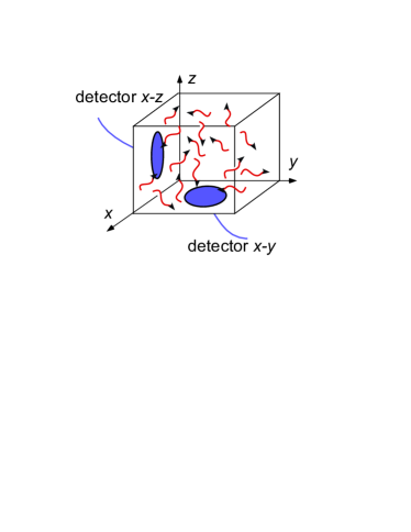
Figure 3: 3D electromagnetic field in a cavity. Detectors are placed on the ($x$, $y$) and ($x$, $z$) planes.

As a result, we determine

$$\lambda_{2} = \frac{1}{2}\left((\Psi_{2}^{(z)})_{t}-\sqrt{2(\Psi_{2}^{(z)2})_{t}-(\Psi_{2}^{(z)})_{t}^{2}}\right),$$

$$I_{z}{\bf u}_{1} = \sqrt{\frac{(\Psi^{(z)}_{2})_{xx}-\lambda_{2}}{\lambda_{1}-\lambda_{2}}}{\bf e}_{x}$$ (33)

$$+ \frac{(\Psi^{(z)}_{2})_{yx}}{\sqrt{(\lambda_{1}-\lambda_{2})((\Psi^{(z)}_{2})_{xx}-\lambda_{2})}}{\bf e}_{y}$$

by means of the known matrix $\Psi_{2}^{(z)}$. From these equations we unambiguously find $\lambda_{2}$ and direction of the vector $I_{z}{\bf u}_{1}/|I_{z}{\bf u}_{1}|$.

Complete retrieval of the 3D coherence matrix requires knowing the vector in 3D space, i.e. measurements out of the plane ($x$, $y$). If we put a detector in the plane ($x$, $z$), using the coherence matrix

$$\Psi_{2}^{(y)}=(\lambda_{1}-\lambda_{2})(I_{y}{\bf u}_{1})\otimes(I_{y}{\bf u}_{1}^{\ast})+\lambda_{2}I_{y}$$ (34)

we can write another projection of the vector ${\bf u}_{1}$

$$I_{y}{\bf u}_{1}=\sqrt{\frac{(\Psi^{(y)}_{2})_{xx}-\lambda_{2}}{\lambda_{1}-\lambda_{2}}}{\bf e}_{x}+\frac{(\Psi^{(y)}_{2})_{zx}}{\sqrt{(\lambda_{1}-\lambda_{2})((\Psi^{(y)}_{2})_{xx}-\lambda_{2})}}{\bf e}_{z}.$$

Then the vector under search is

$${\bf u}_{1}=I_{z}{\bf u}_{1}+{\bf e}_{z}({\bf e}_{z}I_{y}{\bf u}_{1})$$ (35)

or in the explicit form

$${\bf u}_{1}=\sqrt{\frac{(\Psi^{(z)}_{2})_{xx}-\lambda_{2}}{\lambda_{1}-\lambda_{2}}}{\bf e}_{x}+\frac{(\Psi^{(z)}_{2})_{yx}}{\sqrt{(\lambda_{1}-\lambda_{2})((\Psi^{(z)}_{2})_{xx}-\lambda_{2})}}{\bf e}_{y}$$

$$+\frac{(\Psi^{(y)}_{2})_{zx}}{\sqrt{(\lambda_{1}-\lambda_{2})((\Psi^{(y)}_{2})_{xx}-\lambda_{2})}}{\bf e}_{z}.$$ (36)

$\lambda_{2}$ has been found from the in-plane measurement, while $\lambda_{1}$ (and the final form of ${\bf u}_{1}$) follows from the normalization condition $|{\bf u}_{1}|=1$ as

$$\lambda_{1}=\lambda_{2}+|(\Psi^{(z)}_{2})_{xx}-\lambda_{2}|+\frac{|(\Psi^{(z)}_{2})_{yx}|^{2}}{|(\Psi^{(z)}_{2})_{xx}-\lambda_{2}|}+\frac{|(\Psi^{(y)}_{2})_{zx}|^{2}}{|(\Psi^{(y)}_{2})_{xx}-\lambda_{2}|}.$$

Thus we reconstruct the three-dimensional beam tensor (coherence matrix) described by Eq. (8). The degree of polarization for the three-dimensional light follows from Eq. (13).

VI Conclusion

We have derived the light beam tensor (coherence matrix) for three-dimensional fields grounding on the expected symmetry properties: beam’s tensor should not change for rotations with respect to the direction of the fully polarized light. Such a restricted form of the coherence matrix is justified by the definition of the fully polarized light as sum of equiprobably polarized elementary waves. General form of coherence matrix deals with the limited number of unpolarized beams and does not allow determining the actual structure of the field in principle. That is why it is not a great simplification to treat partially polarized light as superposition of coherent field and 3D random field. All the more so considered beam tensor (8) has clear meaning and can be described by 6 independent parameters — Stokes parameters. For the three dimensional light it is natural to choose 6 physical parameters: 3 intensities in different planes and 3 spin angular momenta. We call these values “physical Stokes parameters.” Finally, we have developed the procedure of reconstruction of the 3D light beam tensor using the measurements of the 2D coherence matrices of projected fields.

In some situations it may be not really necessary to introduce the 3D coherence matrix at all. Indeed, if we define the plane of detector as distinguished interface (like the plane of constant phase in 2D case), then we can calibrate the degree of polarization for the 3D beams with respect to this interface. Some different beams may have the same degree of polarizations, though the beams should be different. Only if it is crucial for the results, the full reconstruction of the 3D coherence matrix and calculation of the 3D degree of polarization is needed.

References

- (1) G.A. Siviloglou, J. Broky, A. Dogariu, and D.N. Christodoulides, Phys. Rev. Lett. 99, 213901 (2007).
- (2) J. Chen, J. Ng, Z. Lin, and C.T. Chan, Nat. Photon. 5, 531–534 (2011).
- (3) A. Novitsky, C.-W. Qiu, and H. Wang, Phys. Rev. Lett. 107, 203601 (2011).
- (4) S. Sukhov and A. Dogariu, Phys. Rev. Lett. 107, 203602 (2011).
- (5) W.T.M. Irvine and D. Bouwmeester, Nat. Phys. 4, 716–720 (2008).
- (6) G. Milione, H.I. Sztul, D.A. Nolan, and R.R. Alfano, Phys. Rev. Lett. 107, 053601 (2011).
- (7) H. Poincare, Theorie mathematique de la Lumiere (Paris: Georges Carre, 1892).
- (8) G.G. Stokes, Trans. Cambridge Phil. Soc. 9, 399–416 (1852).
- (9) E. Wolf, Nuovo Cimento 12, 884–888, 1954a.
- (10) R.C. Jones, J. Opt. Soc. Am. 31, 488–493 (1941).
- (11) H. Mueller, J. Opt. Soc. Am. 38, 661 (1948).
- (12) F.I. Fedorov, Zh. Prikl. Spectrosk. 2, 523–533 (1965).
- (13) F.I. Fedorov, Theory of Gyrotropy (Minsk: Nauka i Technika, 1976).
- (14) T. Setala, A. Shevchenko, M. Kaivola, and A.T. Friberg, Phys. Rev. E 66, 016615 (2002).
- (15) T. Setl, K. Lindfors, and A.T. Friberg, Opt. Lett., 34, 3394–3396 (2009).
- (16) J. Ellis, A. Dogariu, S. Ponomarenko, and E. Wolf, Opt. Commun. 248, 333–337 (2005).
- (17) J. Ellis and A. Dogariu, Opt. Commun. 253, 257–265 (2005).
- (18) J. Ellis, A. Dogariu, S. Ponomarenko, and E. Wolf, Opt. Lett. 29, 1536–1538 (2004).
- (19) C. Brosseau and A. Dogariu, Progress in Optics 49, 315–380 (2006).
- (20) Philippe Refregier, Opt. Lett. 37, 428–430 (2012).
- (21) J.M. Aunon and M. Nieto-Vesperinas, Opt. Lett. 38, 58–60 (2013).
- (22) J. Ellis and A. Dogariu, Phys. Rev. Lett. 95, 203905 (2005).