Quantile and quantile-function estimations under density ratio model

Abstract

Population quantiles and their functions are important parameters in many applications. For example, the lower quantiles often serve as crucial quality indices for forestry products. Given several independent samples from populations satisfying the density ratio model, we investigate the properties of empirical likelihood (EL) based inferences. The induced EL quantile estimators are shown to admit a Bahadur representation that leads to asymptotically valid confidence intervals for functions of quantiles. We rigorously prove that EL quantiles based on all the samples are more efficient than empirical quantiles based on individual samples. A simulation study shows that the EL quantiles and their functions have superior performance when the density ratio model assumption is satisfied and when it is mildly violated. An example is used to demonstrate the new method and the potential cost savings.

T1Supported in part by a Collaborative Research and Development grant from Natural Science and Engineering Research Council of Canada and in-kind contributions from Natural Resources Canada (Canadian Forest Service) through FPInnovation’s national research program.

and t2Supported by the NNSF of China, 11001083 and 11101156.

1 Introduction

Forestry plays a major role in the Canadian economy; maintaining the high quality of wood products is vital economically and socially. We are designing an effective long-term monitoring plan for the quality of forestry products in Canada. Two important quality indices for a piece of lumber are the modulus of elasticity (MOE) and the modulus of rupture (MOR), its strength in terms of elasticity and toughness. The reliability of lumber-based structures may depend heavily on the lower population quantiles of these indices. However, it is costly, time consuming and laborious to obtain these quality measurements. Therefore, efficient estimates of the population quantiles and their functions are important.

The estimation of quantiles based on a single random sample is a well-researched topic. Empirical quantiles have been shown to admit a Bahadur representation [Bahadur (1966); Kiefer (1967); Serfling (1980)], making it simple to study the joint limiting distributions of any number of sample quantiles and their smooth functions. In the presence of auxiliary information, the empirical likelihood [EL; Owen (1988, 2001)] can be utilized to improve efficiency. The Bahadur representation of EL estimators has been established by Chen and Chen (2000). There is also an abundant literature on the Bahadur representation when the samples are not independent or have a time-series structure. See Wu (2005) and Zhou and Wu (2009) for recent examples.

In the targeted application, we potentially have a number of random samples from similar populations, and the combined sample size is large. Even if the size of each random sample is small, the total sample size increases over time. We may also have samples from similar products, such as lumber of various shapes and lengths. If the population distributions have some common features, the pooled information may improve the efficiency of each quantile estimate.

Specifically, we study quantile estimators based on the density ratio model (DRM) of Anderson (1979) and the EL approach, and we focus on investigating their properties. Suppose we have $m+1$ independent random samples from populations with cumulative distribution and density functions denoted $G_{k}(x)$ and $g_{k}(x)$, $k=0,1,\ldots,m$. The DRM postulates that

$$\log\bigl{\{}g_{k}(x)/g_{0}(x)\bigr{\}}=\bolds{\theta}_{k}^{\tau}\mathbf{q}(x)$$ (1)

for some known function $\mathbf{q}(x)$ of dimension $d$ and corresponding unknown vector-valued parameters $\bolds{\theta}_{k}$. We require the first element of $\mathbf{q}(x)$ to be one so that the first element of $\bolds{\theta}_{k}$ is a normalization parameter.

In this formulation, the form of $g_{0}(x)$ is unspecified. Many parametric distribution families including normal and Gamma are special cases of the DRM. Qin and Zhang (1997) showed that the logistic regression model commonly used in case–control studies can be described by the DRM. They studied the EL approach for parameter estimation and for goodness-of-fit tests of the regression model. Zhang (2000, 2002) investigated the EL approach for quantile estimation and goodness-of-fit. Fokianos et al. (2001) used the EL approach under the DRM for a classical one-way analysis-of-variance.

We focus on DRM-based quantile estimation and study its Bahadur representation. We show that the EL quantiles are more efficient than empirical quantiles. The representation is then used to construct confidence intervals for the quantiles and their functions. These results are particularly relevant for the design of a long-term monitoring system for wood products. The finite-sample performance of the new methods is superior to that of the empirical quantiles when the DRM model assumption is valid and when it is mildly violated.

In Section 2, we review the EL approach under the DRM. Section 3 derives the Bahadur representation. In Section 4, we study the asymptotic properties of the new quantile estimates. The finite-sample performance is examined in Section 5, and the proposed quantile estimation is illustrated using lumber data in Section 6. The proofs are given in the Appendix.

2 Empirical likelihood under DRM

Empirical likelihood under the DRM can be found in Qin and Zhang (1997) or Fokianos et al. (2001). Suppose the population distributions, $G_{k}(x)$, of $m+1$ random samples of sizes $n_{k}$: $\{(x_{kj}\dvtx j=1,\ldots,n_{k});k=0,1,2,\ldots,m\}$ satisfy the DRM (1). The model assumption may also be written

$$dG_{k}(x)=\exp\bigl{\{}\bolds{\theta}^{\tau}_{k}\mathbf{q}(x)\bigr{\}}\,dG_{0}(x).$$

If $G$ is discrete, then $dG(x)=G(x)-G(x_{-})=P(X=x)$ for the corresponding random variable $X$. The EL is defined as if the $G$’s are discrete. Let $p_{kj}=dG_{0}(x_{kj})$ for all $k,j$. The EL is defined as

$$L_{n}(G_{0},G_{1},\ldots,G_{m})=\prod_{k,j}\,dG_{k}(x_{kj})=\biggl{\{}\prod_{k,j}p_{kj}\biggr{\}}\times\exp\biggl{\{}\sum_{k,j}\bolds{\theta}_{k}^{\tau}\mathbf{q}(x_{kj})\biggr{\}},$$

where the product and summation with respect to $\{k,j\}$ are over the full range: $k=0,\ldots,m$ and $j=1,\ldots,n_{k}$. We set $\bolds{\theta}_{0}=0$ for notational simplicity.

The DRM assumption implies that $L_{n}$ is also a function of the parameter vector $\bolds{\theta}^{\tau}=(\bolds{\theta}_{1}^{\tau},\ldots,\bolds{\theta}_{m}^{\tau})$ and $G_{0}$. Hence, we may also write its logarithm as

$$\ell_{n}(\bolds{\theta},G_{0})=\sum_{k,j}\log(p_{kj})+\sum_{k,j}\bolds{\theta}_{k}^{\tau}\mathbf{q}(x_{kj}).$$

The model assumption also implies that, for $r=0,1,\ldots,m$,

$$\int\exp\bigl{\{}\bolds{\theta}_{r}^{\tau}\mathbf{q}(x)\bigr{\}}\,dG_{0}(x)=1.$$ (2)

Thus, for any $r$ between 0 and $m$, $\sum_{k,j}p_{kj}\exp\{\bolds{\theta}_{r}^{\tau}\mathbf{q}(x_{kj})\}=1,$ which is naturally accommodated in the EL approach.

Inference on $\bolds{\theta}$ and other aspects of the population distributions is usually carried out by first profiling the EL with respect to $\bolds{\theta}$. That is, we define $\tilde{\ell}_{n}(\bolds{\theta})=\max_{G_{0}}\ell_{n}(\bolds{\theta},G_{0})$ subject to constraints (2) on $G_{0}$. Technically, we confine the support of $G_{0}$ to $\{x_{kj}\}$. The maximum in $G_{0}$ is attained when

$$p_{kj}=n^{-1}\Biggl{\{}1+\sum_{s=1}^{m}\nu_{s}\bigl{[}\exp\bigl{\{}\bolds{\theta}_{s}^{\tau}\mathbf{q}(x_{kj})\bigr{\}}-1\bigr{]}\Biggr{\}}^{-1},$$

where $(\nu_{1},\nu_{2},\ldots,\nu_{m})$ is the solution to $\sum_{k,j}p_{kj}\exp\{\bolds{\theta}^{\tau}_{r}\mathbf{q}(x_{kj})\}=1$ for $r=1,2,\ldots,m$ and $n=\sum_{k=0}^{m}n_{k}$ is the total sample size. The profile log-EL (up to an additive constant) is given by

$$\tilde{\ell}_{n}(\bolds{\theta})=-\sum_{k,j}\log\Biggl{\{}1+\sum_{s=1}^{m}\nu_{s}\bigl{[}\exp\bigl{\{}\bolds{\theta}_{s}^{\tau}\mathbf{q}(x_{kj})\bigr{\}}-1\bigr{]}\Biggr{\}}+\sum_{k,j}\bolds{\theta}_{k}^{\tau}\mathbf{q}(x_{kj}).$$ (3)

We may regard $\tilde{\ell}_{n}(\bolds{\theta})$ as a parametric likelihood and activate the classical likelihood-based statistical inference. This profile likelihood has the same maximum value and point as another function,

$$\ell_{n}(\bolds{\theta})=-\sum_{k,j}\log\Biggl{[}\sum_{r=0}^{m}\rho_{r}\exp\bigl{\{}\bolds{\theta}_{r}^{\tau}\mathbf{q}(x_{kj})\bigr{\}}\Biggr{]}+\sum_{k,j}\bolds{\theta}_{k}^{\tau}\mathbf{q}(x_{kj}),$$ (4)

with $\rho_{r}=n_{r}/n$. Because of its simplicity, the literature often regards $\ell_{n}(\bolds{\theta})$ instead of $\tilde{\ell}_{n}(\bolds{\theta})$ as the profile likelihood function of $\bolds{\theta}$. In the two-sample situation, Keziou and Leoni-Aubin (2008) found that it is a “dual likelihood.” Its likelihood ratio statistics remain asymptotically chi-square.

We define the maximum EL estimator (MELE) $\hat{\bolds{\theta}}$ of $\bolds{\theta}$ as the maximum point of (3) or equivalently of (4). The asymptotic normality of $\hat{\bolds{\theta}}$ has been established in various situations [Qin and Zhang (1997); Fokianos et al. (2001); Zhang (2002)]. We summarize and extend these results, giving the necessary details as a preparational step. Let $h(x;\bolds{\theta})=\sum_{k=0}^{m}\rho_{k}\exp\{\bolds{\theta}_{k}^{\tau}\mathbf{q}(x)\},$ and for $k=0,1,\ldots,m$, we define

$$h_{k}(x;\bolds{\theta})=\rho_{k}\exp\bigl{\{}\bolds{\theta}_{k}^{\tau}\mathbf{q}(x)\bigr{\}}/h(x;\bolds{\theta}).$$

Let $\mathbf{h}(x;\bolds{\theta})=\{h_{0}(x;\bolds{\theta}),\ldots,h_{m}(x;\bolds{\theta})\}^{\tau}$ and define an $(m+1)\times(m+1)$ matrix

$$\mathbf{H}(x;\bolds{\theta})=\operatorname{diag}\bigl{\{}\mathbf{h}(x;\bolds{\theta})\bigr{\}}-\mathbf{h}(x;\bolds{\theta})\mathbf{h}^{\tau}(x;\bolds{\theta}).$$

When $\bolds{\theta}=\bolds{\theta}^{*}$, the true value of $\bolds{\theta}$, we may drop $\bolds{\theta}^{*}$ for notational simplicity. Finally, we use $d\bar{G}(x)$ for $h(x;\bolds{\theta}^{*})\,dG_{0}(x)$ in the integrations.

Theorem 2.1

Suppose we have an independent random sample $\{x_{kj}\}_{j=1}^{n_{k}}$ from population $G_{k}$ for $k=0,1,\ldots,m$. The total sample size $n=\sum_{k}n_{k}\to\infty$, and $\rho_{k}=n_{k}/n$ remains a constant (or within the $n^{-1}$ range).

The population distributions $G_{k}$ satisfy the DRM (1) with true parameter value $\bolds{\theta}^{*}$ and $\int h(x;\bolds{\theta})\,dG_{0}<\infty$ in a neighborhood of $\bolds{\theta}^{*}$. The components of $\mathbf{q}(x)$ are linearly independent and its first element is one.

Then $\sqrt{n}(\hat{\bolds{\theta}}-\bolds{\theta}^{*})$ is asymptotically multivariate normal with mean $\mathbf{0}$ and covariance matrix $\mathbf{W}^{-1}-\mathbf{S}$. Both $\mathbf{W}$ and $\mathbf{S}$ are $md\times md$ block matrices with each block a $d\times d$ matrix, and their $(r,s)$th blocks are, respectively,

$$\mathbf{W}_{rs} = \int\mathbf{q}(x)\mathbf{q}^{\tau}(x)\bigl{\{}h_{r}(x)\delta_{rs}-h_{r}(x)h_{s}(x)\bigr{\}}\,d\bar{G}(x),$$

$$\mathbf{S}_{rs} = \bigl{(}\rho_{r}^{-1}\delta_{rs}+\rho_{0}^{-1}\bigr{)}\operatorname{diag}\{1,0,\ldots,0\},$$

where $1\leq r,s\leq m$ and $\delta_{rs}=1$ if $r=s$ and 0 otherwise.

The Appendix contains a sketched proof to bridge some gaps. Using the Kronecker product $\otimes$, we have a tighter expression,

$$\mathbf{W}=\int\mathbf{H}{[-1,-1]}(x)\otimes\bigl{\{}\mathbf{q}(x)\mathbf{q}^{\tau}(x)\bigr{\}}\,d\bar{G}(x),$$ (5)

where $\mathbf{H}{[-1,-1]}(x)$ is $\mathbf{H}(x)$ with its first row and column removed. This convention is adopted from the statistical software package [R Development Core Team (2011)].

The asymptotic normality is a stepping stone for our main result on the Bahadur representation. It also reveals that the MELE is root-$n$ consistent. The assumption that $\int h(x;\theta)\,dG_{0}<\infty$ in a neighborhood of $\bolds{\theta}^{*}$ implies the existence of the moment generating function of $\mathbf{q}(x)$ and therefore all its finite moments. This fact will be used in our proofs.

3 Bahadur representation and its applications

Given the MELE $\hat{\bolds{\theta}}$, the fitted values of $p_{kj}$ are $\hat{p}_{kj}=\{nh(x_{kj};\hat{\bolds{\theta}})\}^{-1}$ and the fitted $G_{r}$ is

$$\hat{G}_{r}(x) = \sum_{k,j}\hat{p}_{kj}\exp\bigl{\{}\hat{\bolds{\theta}}_{r}^{\tau}\mathbf{q}(x_{kj})\bigr{\}}I(x_{kj}\leq x)$$

$$= n_{r}^{-1}\sum_{k,j}h_{r}(x_{kj};\hat{\bolds{\theta}})I(x_{kj}\leq x)$$

with $\hat{\bolds{\theta}}_{0}=0$ and $I(A)$ an indicator function of event $A$. For any $\alpha\in(0,1)$, define the $\alpha$-quantile of $G_{r}$ as $\xi_{r}=\xi_{r,\alpha}=\inf\{x\dvtx G_{r}(x)\geq\alpha\}$ and its EL-based estimator as

$$\hat{\xi}_{r}=\hat{\xi}_{r,\alpha}=\inf\bigl{\{}x\dvtx\hat{G}_{r}(x)\geq\alpha\bigr{\}}.$$ (6)

We call the $\hat{\xi}_{r}$ values EL quantiles for simplicity. The asymptotic normality of the EL quantile $\hat{\xi}_{r}$ is useful for constructing confidence intervals for $\xi_{r}$ or for testing related hypotheses. Researchers are often interested in smooth functions of quantiles of many populations and/or at several levels. Thus, the multivariate asymptotic behavior is useful, and this calls for the Bahadur representation.

Theorem 3.1

Assume the conditions of Theorem 2.1, and that the density function $g_{r}(x)$ is continuous and positive at $x=\xi_{r}$. The EL quantile (6) has Bahadur representation

$$\hat{\xi}_{r}=\xi_{r}+\bigl{\{}{\alpha}-\hat{G}_{r}(\xi_{r})\bigr{\}}/g_{r}(\xi_{r})+O_{p}\bigl{(}n^{-3/4}\bigl{\{}\log(n)\bigr{\}}^{1/2}\bigr{)},$$ (7)

where $\xi_{r}$ is the $\alpha$th quantile of $G_{r}(x)$.

The proof is given in the Appendix. Without the Bahadur representation, it is a daunting task to derive the limiting distribution of functions of EL quantiles such as $\hat{\xi}_{0,\alpha}-\hat{\xi}_{1,\alpha}$. Theorem 3.1 links this task to that of $\{a\hat{G}_{0}(\xi_{0,\alpha})-b\hat{G}_{1}(\xi_{1,\alpha})\}$ with nonrandom constants $a$ and $b$. The asymptotic properties of $\hat{G}_{r}$ are simple and easy to use.

Theorem 3.2

Assume the same conditions as in Theorem 2.1. For any $0\leq r_{1},r_{2},\ldots,r_{k}\leq m$ and an accompanying set of real numbers $x_{1},x_{2},\ldots,x_{k}$ in the support of $G_{0}(x)$, $\sqrt{n}\{\hat{G}_{r_{j}}(x_{j})-G_{r_{j}}(x_{j})\}$ are jointly asymptotically $k$-variate normal with mean $\mathbf{0}$ and covariance matrix $\Omega_{\operatorname{EL}}=(\omega_{r_{i},r_{j}}(x_{i},x_{j}))_{1\leq i,j\leq k}$. The generic form of $\omega_{r_{i},r_{j}}(x_{i},x_{j})$ is given by

$$\omega_{rs}(x,y)=\sigma_{rs}(x,y)-(\rho_{r}\rho_{s})^{-1}\bigl{\{}a_{rs}(x\wedge y)-\mathbf{B}_{r}^{\tau}(x)\mathbf{W}^{-1}\mathbf{B}_{s}(y)\bigr{\}},$$ (8)

where $x\wedge y=\min\{x,y\}$,

$$\sigma_{rs}(x,y) = \rho_{r}^{-1}\delta_{rs}\bigl{\{}G_{r}(x\wedge y)-G_{r}(x)G_{s}(y)\bigr{\}},$$

$$a_{rs}(x) = \int_{-\infty}^{x}\bigl{\{}\delta_{rs}h_{r}(t)-h_{r}(t)h_{s}(t)\bigr{\}}\,d\bar{G}(t)$$

and $\mathbf{B}_{r}(x)$ is a vector of length $md$ with its $s$th segment (of length $d$ with $s=1,2,\ldots,m$) being

$$\mathbf{B}_{r,s}(x)=\int_{-\infty}^{x}\bigl{\{}\delta_{rs}h_{r}(t)-h_{r}(t)h_{s}(t)\bigr{\}}\mathbf{q}(t)\,d\bar{G}(t).$$

The proof is given in the Appendix. The Bahadur representation (7) and the multivariate asymptotic normality of the $\hat{G}$’s lead to multivariate asymptotic normality of the EL quantiles. For notational simplicity, we will state the result only for the bivariate case. Let $\xi_{r}$ be the population quantile at some level $\alpha_{r}$ of the $r$th population in the DRM. We similarly define $\xi_{s}$ at some level $\alpha_{s}$. The exact levels $\alpha_{r}$ and $\alpha_{s}$ are not important.

Theorem 3.3

Assume that the conditions in Theorem 3.1 hold for $\xi_{r}$ and $\xi_{s}$. The centralized EL quantile under the DRM assumption

$$\sqrt{n}(\hat{\xi}_{r}-\xi_{r},\hat{\xi}_{s}-\xi_{s})$$

is asymptotically bivariate normal with mean 0 and covariance matrix

$$\Sigma_{\operatorname{EL}}=\pmatrix{\omega_{rr}(\xi_{r},\xi_{r})/g_{r}^{2}(\xi_{r})&\omega_{rs}(\xi_{r},\xi_{s})/\bigl{\{}g_{r}(\xi_{r})g_{s}(\xi_{s})\bigr{\}}\vspace*{2pt}\cr\omega_{rs}(\xi_{r},\xi_{s})/\bigl{\{}g_{r}(\xi_{r})g_{s}(\xi_{s})\bigr{\}}&\omega_{ss}(\xi_{s},\xi_{s})/g_{s}^{2}(\xi_{s})}.$$ (9)

The above result does not restrict the selection of the two populations or the levels of the quantiles. It can be used to conveniently obtain the limiting distributions of smooth functions of the EL quantiles.

4 Efficiency comparison

The EL quantiles are constructed by pooling information from $m+1$ independent random samples. We trust that they are more efficient than empirical quantiles (hereafter EM) based on single samples. A rigorous proof of this intuitive claim is not simple.

Let $\breve{G}_{r}(x)$ be the empirical distribution function based solely on the $r$th sample. As processes indexed by $x$, $\sqrt{n}\{\breve{G}_{r}(x)-G_{r}(x)\}$, $r=0,1,\ldots,m$, are independent and each converges in distribution to a Gaussian process with covariance function $\sigma_{rr}(x,x)$. Let $\breve{\xi}_{r}$ be the EM quantiles of the $r$th population at level $\alpha_{r}$. Based on the classical Bahadur presentation, with any number of choices in $r$ and $\alpha_{r}$, $\{\sqrt{n}(\breve{\xi}_{r}-\xi_{r})\}$ are jointly asymptotically multivariate normal with mean 0. In the bivariate case, the asymptotic covariance matrix of $\sqrt{n}(\breve{\xi}_{r}-\xi_{r},\breve{\xi}_{s}-\xi_{s})$ is given by

$$\Sigma_{\operatorname{EM}}=\pmatrix{\sigma_{rr}(\xi_{r},\xi_{r})/\bigl{\{}g_{r}^{2}(\xi_{r})\bigr{\}}&\sigma_{rs}(\xi_{r},\xi_{s})/\bigl{\{}g_{r}(\xi_{r})g_{s}(\xi_{s})\bigr{\}}\vspace*{2pt}\cr\sigma_{sr}(\xi_{s},\xi_{r})/\bigl{\{}g_{r}(\xi_{r})g_{s}(\xi_{s})\bigr{\}}&\sigma_{ss}(\xi_{s},\xi_{s})/\bigl{\{}g_{s}^{2}(\xi_{s})\bigr{\}}},$$

where $\sigma_{rs}(x,y)$ was given in Theorem 3.2.

Since the EL and EM quantiles are asymptotically unbiased, the efficiency comparison reduces to a comparison of two asymptotic covariance matrices. The following result generalizes Corollary 4.3 of Zhang (2000).

Theorem 4.1

For any pair of integers $0\leq r,s\leq m$ and any quantile levels $\alpha_{r}$ and $\alpha_{s}$, we have $\Sigma_{\operatorname{EM}}-\Sigma_{\operatorname{EL}}\geq 0$. This conclusion remains true for any number of quantiles.

5 Inferences on functions of quantiles

In applications such as the wood project, we are interested in the size of $\xi_{r}$, $\xi_{r}-\xi_{s}$, etc. for various choices of $r$ and $s$ and various levels. Two scenarios are of particular interest. (A) For a specific wood product in a given year, is its quality index above or below the industrial standard? (B) How different are the quality indices for wood products produced in two different years, mills or regions?

(A) and (B) can be addressed through hypothesis tests or the construction of confidence intervals. With the asymptotic normality and favorable efficiency properties of the EL quantiles, the task is simple. We must find a consistent estimate of $\operatorname{var}(\hat{\xi}_{r})$ and construct approximate $100(1-\alpha)\%$ confidence intervals as $\hat{\xi}_{r}\pm z_{\alpha/2}\sqrt{\hat{\operatorname{var}}(\hat{\xi}_{r})},$ where $z_{{\alpha/2}}$ denotes the $(1-{\alpha}/{2})$th quantile of the standard normal distribution. Similarly, approximate confidence intervals for $\xi_{r}-\xi_{s}$ are $(\hat{\xi}_{r}-\hat{\xi}_{s})\pm z_{\alpha/2}\sqrt{\hat{\operatorname{var}}(\hat{\xi}_{r}-\hat{\xi}_{s})}.$ In both cases, we need effective and consistent estimates of $\operatorname{var}(\hat{\xi}_{r})$ and $\operatorname{var}(\hat{\xi}_{r}-\hat{\xi}_{s})$.

With the help of (9), plug-in consistent variance estimators can easily be constructed. Two necessary ingredients are consistent estimations of $\omega_{rs}(x,y)$ and $g_{r}(x)$. Although $\hat{G}_{r}(x)$ is discrete, the idea of kernel density estimation can be used to produce a density estimate. Let $K(\cdot)\geq 0$ be a commonly used kernel function such that $\int K(x)\,dx=1$, $\int xK(x)\,dx=0$ and $\int x^{2}K(x)\,dx<\infty$. For some bandwidth $b>0$, let $K_{b}(x)=(1/b)K(x/b).$ Then a kernel estimate of $g_{r}(x)$ is given by

$$\hat{g}_{r}(x)=\int K_{b}(x-y)\,d\hat{G}_{r}(y).$$

In the simulation study, we set $K(x)$ to the standard normal density function. We chose the bandwidth $b$ according to the rule of thumb of Deheuvels (1977) and Silverman (1986),

$$b=1.06n^{-1/5}\min\{\hat{\sigma},\hat{R}/1.34\}.$$

The above formula is designed for the situation where the density function is estimated based on $n$ independent and identically distributed observations. In our simulation, we regard the fitted $\hat{G}_{r}(x)$ as a nonrandom distribution function, and compute the standard deviation and inter-quartile range of this distribution as $\hat{\sigma}$ and $\hat{R}$.

The analytical form of $\omega_{rs}(x,y)$ contains many terms, but it is straightforward to estimate them consistently and sensibly. Let

$$\hat{a}_{rs}(x)=\int_{-\infty}^{x}\bigl{\{}\delta_{rs}h_{r}(t;\hat{\bolds{\theta}})-h_{r}(t;\hat{\bolds{\theta}})h_{s}(x;\hat{\bolds{\theta}})\bigr{\}}h(t;\hat{\bolds{\theta}})\,d\hat{G}_{0}(t),$$

and we form $\hat{\mathbf{B}}_{r}(x)$ and $\hat{\mathbf{W}}$ via

$$\hat{\mathbf{B}}_{r,s}(x) = \int_{-\infty}^{x}\bigl{\{}\delta_{rs}h_{r}(t;\hat{\bolds{\theta}})-h_{r}(t;\hat{\bolds{\theta}})h_{s}(x;\hat{\bolds{\theta}})\bigr{\}}\mathbf{q}(t)h(t;\hat{\bolds{\theta}})\,d\hat{G}_{0}(t),$$

$$\hat{\mathbf{W}}_{rs} = \int_{-\infty}^{\infty}\bigl{\{}\delta_{rs}h_{r}(t;\hat{\bolds{\theta}})-h_{r}(t;\hat{\bolds{\theta}})h_{s}(x;\hat{\bolds{\theta}})\bigr{\}}\mathbf{q}(t)\mathbf{q}^{\tau}(t)h(t;\hat{\bolds{\theta}})\,d\hat{G}_{0}(t).$$

We then form a consistent estimator of $\omega_{rs}(\xi_{r},\xi_{s})$ as

$$\hat{\omega}_{rs}(\xi_{r},\xi_{s})=\rho_{r}^{-1}\delta_{rs}(\alpha_{r}-\alpha_{r}\alpha_{s})-(\rho_{r}\rho_{s})^{-1}\bigl{\{}\hat{a}_{rs}(\hat{\xi}_{r}\wedge\hat{\xi}_{s})-\hat{\mathbf{B}}_{r}^{\tau}(\hat{\xi}_{r})\hat{\mathbf{W}}^{-1}\hat{\mathbf{B}}_{s}(\hat{\xi}_{s})\bigr{\}},$$

where we have used the facts that $\delta_{rs}G_{r}(\xi_{r}\wedge\xi_{s})=\delta_{rs}\alpha_{r}$ and $G_{r}(\xi_{r})=\alpha_{r}$.

6 Simulation study

We now examine the finite-sample performance of the inference procedures via simulation. Are the EL quantiles $\hat{\xi}$ more efficient than the EM quantiles $\breve{\xi}$? The simulation studies shed light on how large the sample must be before the asymptotic result applies. We analyze data sets generated from several sets of populations, which are divided into two groups: those that satisfy the DRM assumption and those that do not.

6.1 Populations satisfying DRM assumptions

Recall that the Gamma and normal distribution families are special DRMs. We choose two sets of distributions from these families with the parameter values specified in Table 1. For the Gamma distributions, the first parameter is the degrees of freedom and the second is the scale. Therefore, the expectation of the first population is $6\times 1.5$. The parameters for the normal distribution are the mean and variance. The populations have similar means and variances to those seen in applications.

Table 1: Parameters under DRM

Distributions						$\bolds{\mathbf{q}^{\tau}(x)}$
$\Gamma$(6, 1.5)	$\Gamma$(6, 1.4)	$\Gamma$(7, 1.3)	$\Gamma$(7, 1.2)	$\Gamma$(8, 1.1)	$\Gamma$(8, 1.0)	($1,x,\log(x)$)
$N(18,4)$	$N(18,9)$	$N(20,6)$	$N(20,9)$	$N(22,8)$	$N(22,10)$	($1,x,x^{2}$)

The simulations were carried out with $n_{r}=50$ and 2000 repetitions. We examine the performance of $\hat{G}_{r}(x)$ and $\breve{G}_{r}(x)$ for $x$ set to the quantile levels $\alpha=5\%$, 10%, 50%, 90% and 95%. We computed the relative bias, the asymptotic variance and the simulated variance of the EL estimator $\hat{G}_{r}(x)$. The EM estimator $\breve{G}_{r}(x)$ is unbiased, and its asymptotic variance is $\alpha(1-\alpha)/\rho_{r}$. For ease of comparison, we report the ratios of the EM and EL asymptotic variances and the ratios of their simulated variances. We also report the ratios of the mean estimated variances of $\hat{G}_{r}(x)$ and their corresponding asymptotic variances. The results are presented in Table 2.

Table 2: EL and EM distribution estimates. $\hat{G}$: EL estimate; $\breve{G}$: EM estimate; $\sigma^{2}$: asymptotic variance; $\hat{\sigma}^{2}$: average of variance estimate; ${\mathrm{B}}$: bias of $\sqrt{\alpha(1-\alpha)}$ as percentage; $n_{k}=50$

	$\bolds{\alpha}$	$\bolds{\sigma^{2}(\hat{G})}$	$\bolds{\sigma^{2}(\breve{G})/\sigma^{2}(\hat{G})}$	$\bolds{\operatorname{var}(\breve{G})/\operatorname{var}(\hat{G})}$	$\bolds{\hat{\sigma}^{2}(\hat{G})/\operatorname{var}(\hat{G})}$	$\bolds{{\mathrm{B}}(\hat{G})}$	$\bolds{{\mathrm{B}}(\breve{G})}$
$\Gamma(6,1.5)$	0.05	0.176	1.62	1.48	1.03	$-$0.46	$-$4.02
	0.10	0.378	1.43	1.38	1.00	$-$0.28	$-$3.24
	0.50	1.055	1.42	1.33	0.98	$-$0.65	$-$1.92
	0.90	0.382	1.41	1.38	1.01	$-$0.83	$-$3.68
	0.95	0.178	1.60	1.58	1.12	$-$0.45	$-$4.67
$\Gamma(6,1.4)$	0.05	0.176	1.62	1.49	1.08	$-$1.15	$-$4.37
	0.10	0.374	1.44	1.39	1.03	$-$0.71	$-$3.33
	0.50	1.031	1.45	1.37	1.00	$-$0.31	$-$2.03
	0.90	0.370	1.46	1.39	1.04	$-$0.68	$-$3.20
	0.95	0.172	1.66	1.66	1.13	$-$0.74	$-$4.39
$\Gamma(7,1.3)$	0.05	0.170	1.67	1.50	1.00	$-$0.27	$-$4.18
	0.10	0.368	1.47	1.49	1.04	$-$0.20	$-$2.74
	0.50	1.034	1.45	1.44	0.98	$-$0.29	$-$1.74
	0.90	0.394	1.37	1.39	1.01	$-$0.24	$-$3.12
	0.95	0.186	1.53	1.60	1.07	$-$0.29	$-$4.33
$\Gamma(7,1.2)$	0.05	0.171	1.67	1.56	1.06	$-$0.86	$-$4.14
	0.10	0.369	1.46	1.39	1.05	$-$0.78	$-$3.38
	0.50	1.065	1.41	1.32	0.97	$-$0.51	$-$2.33
	0.90	0.371	1.46	1.42	0.99	$-$0.81	$-$3.57
	0.95	0.169	1.68	1.60	0.99	$-$1.13	$-$4.68
$\Gamma(8,1.1)$	0.05	0.172	1.65	1.54	1.06	$-$0.72	$-$4.26
	0.10	0.372	1.45	1.44	1.05	$-$0.67	$-$3.27
	0.50	1.055	1.42	1.43	1.01	$-$0.25	$-$1.53
	0.90	0.373	1.45	1.47	1.01	$-$0.19	$-$3.56
	0.95	0.176	1.62	1.68	1.08	$-$0.37	$-$4.15
$\Gamma(8,1.0)$	0.05	0.180	1.59	1.55	1.07	$-$1.04	$-$4.22
	0.10	0.379	1.42	1.41	0.98	$-$0.81	$-$3.44
	0.50	1.041	1.44	1.33	0.95	$-$0.28	$-$1.63
	0.90	0.364	1.48	1.52	1.09	$-$0.01	$-$2.99
	0.95	0.164	1.73	1.64	1.09	$-$0.64	$-$4.39

Table 3: EL and EM quantiles. $\xi$: true quantile; $\hat{\xi}$: EL quantile; $\breve{\xi}$: EM quantile; $\sigma^{2}$: asymptotic variance; $\hat{\sigma}^{2}$: average of variance estimate; ${\mathrm{B}}$: relative bias as percentage; $n_{k}=50$

	$\bolds{\alpha}$	$\bolds{\xi}$	$\bolds{\sigma^{2}(\hat{\xi})}$	$\bolds{\operatorname{var}(\hat{\xi})}$	$\bolds{\hat{\sigma}^{2}(\hat{\xi})}$	$\bolds{\operatorname{var}(\breve{\xi})/\operatorname{var}(\hat{\xi})}$	$\bolds{\mathrm{B}(\hat{\xi})}$	$\bolds{\mathrm{B}(\breve{\xi})}$
$\Gamma(6,1.5)$	0.05	$3.92$	$71.31$	$70.38$	$67.50$	1.51	$2.19$	$1.59$
	0.10	$4.73$	$69.23$	$68.28$	$73.79$	1.34	$1.08$	$0.97$
	0.50	$8.51$	$83.70$	$88.50$	$94.46$	1.27	$0.45$	$0.15$
	0.90	$13.91$	$298.78$	$292.15$	$287.19$	1.35	$0.23$	$0.19$
	0.95	$15.77$	$473.53$	$468.31$	$469.48$	1.54	$-0.25$	$-0.32$
$\Gamma(6,1.4)$	0.05	$3.66$	$62.34$	$62.42$	$59.15$	1.55	$2.84$	$1.94$
	0.10	$4.41$	$59.63$	$60.02$	$64.02$	1.31	$1.55$	$0.88$
	0.50	$7.94$	$71.30$	$75.64$	$81.58$	1.39	$0.27$	$0.28$
	0.90	$12.98$	$252.32$	$248.04$	$248.28$	1.37	$0.11$	$-0.05$
	0.95	$14.72$	$397.73$	$387.44$	$399.88$	1.51	$-0.05$	$-0.41$
$\Gamma(7,1.3)$	0.05	$4.27$	$67.35$	$66.55$	$62.81$	1.59	$1.83$	$1.07$
	0.10	$5.06$	$63.93$	$64.70$	$68.40$	1.33	$0.88$	$0.50$
	0.50	$8.67$	$72.61$	$76.18$	$82.87$	1.37	$0.30$	$0.04$
	0.90	$13.69$	$260.55$	$254.74$	$241.91$	1.30	$-0.08$	$-0.12$
	0.95	$15.40$	$413.83$	$414.73$	$395.77$	1.52	$-0.22$	$-0.11$
$\Gamma(7,1.2)$	0.05	$3.94$	$57.63$	$59.87$	$54.10$	1.54	$2.32$	$1.11$
	0.10	$4.67$	$54.66$	$56.15$	$58.62$	1.36	$1.32$	$0.75$
	0.50	$8.00$	$63.76$	$65.99$	$70.68$	1.32	$0.30$	$0.23$
	0.90	$12.64$	$208.95$	$229.25$	$206.39$	1.32	$0.24$	$0.12$
	0.95	$14.21$	$320.80$	$340.92$	$319.98$	1.61	$0.13$	$-0.13$
$\Gamma(8,1.1)$	0.05	$4.38$	$60.62$	$56.57$	$54.22$	1.66	$1.95$	$1.07$
	0.10	$5.12$	$56.23$	$54.25$	$58.29$	1.33	$1.12$	$0.63$
	0.50	$8.44$	$61.08$	$60.83$	$67.63$	1.40	$0.23$	$-0.10$
	0.90	$12.95$	$195.71$	$198.99$	$188.42$	1.36	$-0.15$	$-0.03$
	0.95	$14.46$	$309.32$	$323.05$	$295.76$	1.47	$-0.24$	$-0.55$
$\Gamma(8,1.0)$	0.05	$3.98$	$52.12$	$50.42$	$44.41$	1.55	$2.48$	$1.22$
	0.10	$4.66$	$47.38$	$47.27$	$47.85$	1.31	$1.35$	$0.88$
	0.50	$7.67$	$49.81$	$53.38$	$55.67$	1.35	$-0.02$	$0.00$
	0.90	$11.77$	$157.93$	$162.29$	$155.97$	1.33	$-0.22$	$-0.30$
	0.95	$13.15$	$238.30$	$247.86$	$242.16$	1.55	$-0.14$	$-0.32$

There is an efficiency gain in the range of 40% to 70% for the EL estimators in terms of both the theoretical and simulated variances. The variances of the EL estimators are estimated accurately: in the $\hat{\sigma}^{2}(\hat{G})/\sigma^{2}(\hat{G})$ column all the entries are close to 1. Finally, the relative biases $B(\hat{G})$ and $B(\breve{G})$ are both small.

We now turn to investigating the performance of the EL and EM quantiles for both point and interval estimations. The quantile of a discrete distribution $G(x)$ is not a smooth function, and this puts the EM quantile at a disadvantage. To ensure that the EL quantile had a strong competitor, we modified the EM quantile. We replaced $\breve{G}(x)$ by $\breve{G}_{r}(x)-(2n_{r})^{-1}$, and we used linear interpolation to calculate this quantile. These modifications do not alter the first-order asymptotics. We continue to use the notation $\hat{\xi}_{r}$ and $\breve{\xi}_{r}$ for the EL and EM quantiles after these modifications.

The simulation results for the quantile estimates are given in Table 3. The simulated EL variances $\operatorname{var}(\hat{\xi})$ and the mean estimated EL variances $\hat{\sigma}^{2}(\hat{\xi})$ are both close to the asymptotic variances $\sigma^{2}(\hat{\xi})$. The results support the asymptotic theory and the viability of the EL variance estimator. The ratio $\operatorname{var}(\breve{\xi})/\operatorname{var}(\hat{\xi})$ is based on simulated variances and ranges between 1.20 and 1.60. These results indicate an efficiency gain of between 20% and 60% in the EL quantiles. Finally, the relative biases $B(\hat{\xi})$ and $B(\breve{\xi})$ are low and within $\pm 3$%.

The simulation results for the interval estimates of the quantiles and quantile differences are given in Table 4. We compute the average lengths and coverage probabilities of the EL and EM confidence intervals at the $95\%$ level. The coverage probabilities of the EL intervals are almost always closer to the nominal $95\%$. This advantage is more obvious for the upper-tail quantiles (such as the 95% quantile). Often, the coverage gains of the EL intervals reach 5%, and these intervals are 10% to 20% shorter.

Table 4: Confidence intervals for quantile and quantile differences. Nominal level: $95\%$; $\Gamma(6,1.5)-\Gamma(6,1.4)$: differences of $\Gamma(6,1.5)$ and $\Gamma(6,1.4)$ quantilesat the given level; $n_{k}=50$

		EL					EM
	$\bolds{\alpha}$	$\bolds{5\%}$	$\bolds{10\%}$	$\bolds{50\%}$	$\bolds{90\%}$	$\bolds{95\%}$	$\bolds{5\%}$	$\bolds{10\%}$	$\bolds{50\%}$	$\bolds{90\%}$	$\bolds{95\%}$
$\Gamma(6,1.5)$	length	$1.83$	$1.93$	$2.18$	$3.77$	$4.73$	$2.33$	$2.42$	$2.66$	$4.23$	$5.20$
	coverage	$93.0$	$94.8$	$95.2$	$90.7$	$89.5$	$92.3$	$96.5$	$95.9$	$89.1$	$84.9$
$\Gamma(6,1.4)$	length	$1.71$	$1.79$	$2.03$	$3.49$	$4.36$	$2.16$	$2.24$	$2.47$	$3.98$	$4.87$
	coverage	$91.8$	$94.3$	$95.0$	$90.9$	$88.7$	$91.7$	$95.0$	$96.3$	$89.0$	$84.3$
$\Gamma(7,1.3)$	length	$1.76$	$1.85$	$2.03$	$3.41$	$4.27$	$2.25$	$2.31$	$2.48$	$3.88$	$4.78$
	coverage	$92.0$	$93.7$	$95.5$	$92.2$	$90.1$	$90.0$	$95.0$	$96.8$	$90.1$	$85.1$
$\Gamma(7,1.2)$	length	$1.63$	$1.71$	$1.88$	$3.16$	$3.92$	$2.07$	$2.13$	$2.31$	$3.62$	$4.45$
	coverage	$91.9$	$94.3$	$95.3$	$92.5$	$91.3$	$91.3$	$95.5$	$97.4$	$89.4$	$85.1$
$\Gamma(8,1.1)$	length	$1.64$	$1.71$	$1.84$	$3.02$	$3.73$	$2.09$	$2.12$	$2.26$	$3.50$	$4.24$
	coverage	$91.5$	$93.9$	$95.4$	$92.0$	$90.1$	$91.5$	$95.0$	$95.9$	$90.6$	$85.7$
$\Gamma(8,1.0)$	length	$1.50$	$1.56$	$1.67$	$2.74$	$3.36$	$1.91$	$1.93$	$2.05$	$3.15$	$3.82$
	coverage	$90.1$	$93.4$	$95.3$	$92.5$	$91.7$	$89.3$	$94.9$	$96.6$	$90.0$	$85.1$
$\Gamma(6,1.5)-\Gamma(6,1.4)$	length	$2.41$	$2.58$	$2.92$	$5.08$	$6.33$	$3.23$	$3.32$	$3.65$	$5.95$	$7.38$
	coverage	$95.0$	$95.5$	$95.5$	$93.8$	$94.5$	$94.5$	$97.3$	$96.0$	$91.8$	$89.5$
$\Gamma(6,1.5)-\Gamma(7,1.3)$	length	$2.47$	$2.62$	$2.91$	$5.00$	$6.22$	$3.29$	$3.37$	$3.66$	$5.87$	$7.33$
	coverage	$95.1$	$96.1$	$95.3$	$94.8$	$95.1$	$94.1$	$96.8$	$96.2$	$93.2$	$89.9$
$\Gamma(6,1.5)-\Gamma(7,1.2)$	length	$2.37$	$2.53$	$2.82$	$4.89$	$6.09$	$3.17$	$3.25$	$3.54$	$5.69$	$7.09$
	coverage	$93.9$	$95.5$	$95.8$	$94.1$	$93.7$	$94.2$	$96.2$	$96.5$	$93.4$	$90.2$
$\Gamma(6,1.5)-\Gamma(8,1.1)$	length	$2.40$	$2.54$	$2.79$	$4.78$	$5.95$	$3.18$	$3.25$	$3.51$	$5.61$	$6.95$
	coverage	$94.2$	$95.8$	$96.3$	$94.7$	$93.7$	$94.4$	$96.6$	$96.1$	$93.2$	$90.0$
$\Gamma(6,1.5)-\Gamma(8,1.0)$	length	$2.29$	$2.43$	$2.71$	$4.68$	$5.84$	$3.06$	$3.12$	$3.38$	$5.39$	$6.67$
	coverage	$93.5$	$95.2$	$95.9$	$92.3$	$91.9$	$94.1$	$96.4$	$96.7$	$92.7$	$89.0$

We also conducted simulations for the second group of populations, as shown in Table 1, and for $n_{r}=100$. The results are similar and omitted. In conclusion, the EL approach is superior when the model assumptions are satisfied.

6.2 Performance when model is misspecified

What happens to the EL approach when the model is misspecified? Fokianos and Kaimi (2006) quantified the effect of choosing an incorrect linear form of $\mathbf{q}(x)$. In general, both the point estimation and the hypothesis tests are adversely affected when the model is misspecified. These findings may have motivated the model selection approach in Fokianos (2007). That is, instead of pre-specifying a known $\mathbf{q}(x)$, one may select $\mathbf{q}(x)$ as a linear combination of a rich class of functions. For instance, let $\mathbf{q}(x)=\{1,\log x,x^{0.5},x,x^{1.5},x^{2}\}^{\tau}$. The most appropriate $\mathbf{q}(x)$ is then determined by selecting a subvector of the current $\mathbf{q}(x)$. Hence, the classical model selection approaches can be used.

Following this lead, we provide a limited study of the impact of misspecification on the quantile estimations. For this purpose, we simulated random samples from a number of Gamma distributions, Weibull distributions, denoted $W(\cdot,\cdot)$, and normal distributions, as shown in Table 5. These populations are chosen to have similar means and variances. We obtained the EL quantile estimates as if they satisfy DRM for some pre-specified but wrong $\mathbf{q}(x)$.

Table 5: Parameters for non-DRM

$\Gamma$(16, 0.6)	$\Gamma$(19, 0.5)	$N(9,5)$	$N(9.6,5.6)$	$W(10,4.5)$	$W(11,5)$
$\Gamma$(16, 0.6)	$\Gamma$(19, 0.5)	$\Gamma$(17.5, 0.5)	$W(10.5,4.5)$	$W(10,4.5)$	$W(11,5)$

Table 6: EL and EM quantiles under model mis-specification. $\xi$: true quantile; $\hat{\xi}$: EL quantile; $\breve{\xi}$: EM quantile; $\hat{\sigma}^{2}$: average of variance estimate; ${\mathrm{B}}$: relative bias as percentage; $n_{k}=50$

	$\bolds{\alpha}$	$\bolds{\xi}$	$\bolds{\operatorname{mse}(\hat{\xi})}$	$\bolds{\operatorname{mse}(\breve{\xi})/\operatorname{mse}(\hat{\xi})}$	$\bolds{\hat{\sigma}(\hat{\xi})/\operatorname{mse}(\hat{\xi})}$	$\bolds{{\mathrm{B}}(\hat{\xi})}$	$\bolds{{\mathrm{B}}(\breve{\xi})}$
$\Gamma(16,0.6)$	0.05	$6.022$	$61.06$	1.23	0.83	$1.20$	$0.56$
	0.10	$6.681$	$49.19$	1.19	0.95	$0.48$	$0.07$
	0.50	$9.401$	$44.14$	1.16	1.13	$-0.16$	$-0.18$
	0.90	$12.775$	$125.38$	1.10	0.94	$0.24$	$-0.04$
	0.95	$13.858$	$210.07$	1.17	0.92	$0.05$	$-0.27$
$\Gamma(19,0.5)$	0.05	$6.221$	$57.81$	1.22	0.78	$1.29$	$0.71$
	0.10	$6.836$	$44.47$	1.14	0.90	$0.77$	$0.33$
	0.50	$9.334$	$34.15$	1.20	1.17	$0.07$	$0.10$
	0.90	$12.378$	$97.34$	1.14	0.97	$0.17$	$-0.00$
	0.95	$13.346$	$151.68$	1.20	0.98	$0.06$	$-0.40$
$N(9,5)$	0.05	$5.322$	$103.06$	1.23	0.85	$1.43$	$0.77$
	0.10	$6.134$	$73.47$	1.08	0.94	$0.17$	$0.23$
	0.50	$9.000$	$37.86$	1.20	1.14	$0.21$	$-0.03$
	0.90	$11.866$	$68.81$	1.18	0.92	$-0.26$	$-0.17$
	0.95	$12.678$	$97.39$	1.30	0.89	$-0.39$	$-0.39$
$N(9.6,5.6)$	0.05	$5.708$	$116.53$	1.25	0.89	$0.79$	$0.49$
	0.10	$6.567$	$87.51$	1.14	0.90	$0.18$	$0.13$
	0.50	$9.600$	$43.71$	1.20	1.11	$0.37$	$0.27$
	0.90	$12.633$	$76.92$	1.22	0.96	$-0.06$	$-0.13$
	0.95	$13.492$	$112.45$	1.25	0.91	$-0.26$	$-0.30$
$W(10,4.5)$	0.05	$3.344$	$12.09$	1.01	0.85	$0.89$	$0.48$
	0.10	$3.593$	$6.62$	1.01	0.97	$0.58$	$0.20$
	0.50	$4.338$	$2.08$	1.10	1.11	$-0.09$	$-0.01$
	0.90	$4.891$	$1.91$	1.17	1.14	$-0.01$	$-0.11$
	0.95	$5.022$	$2.17$	1.39	1.17	$0.13$	$-0.18$
$W(11,5.0)$	0.05	$3.817$	$11.89$	1.15	0.94	$0.79$	$0.25$
	0.10	$4.075$	$6.67$	1.11	0.94	$0.56$	$0.01$
	0.50	$4.836$	$1.99$	1.16	1.14	$-0.09$	$-0.03$
	0.90	$5.394$	$2.15$	1.03	1.18	$-0.11$	$-0.07$
	0.95	$5.524$	$2.63$	1.14	1.18	$0.05$	$-0.08$

As a trade-off between model interpretation and parsimony, we choose $\mathbf{q}(x)=(1,x,\log(1+|x|),\sqrt{|x|})^{\tau}$. The remaining settings are the same as before. In Table 6, we report only the biases and mean square errors (mse) of the EL and EM quantiles. The EL quantiles are still uniformly more efficient with the efficiency gains usually above 15%. The variance estimators remain accurate, and the relative biases $B(\hat{\xi})$ and $B(\breve{\xi})$ are still negligible.

The simulation results for the interval estimates of the quantiles and quantile differences are given in Table 7. We compute the average lengths and the coverage probabilities of the EL and EM confidence intervals at the $95\%$ level. The EL confidence intervals are not clearly better. These intervals have better coverage probabilities for the upper quantiles but similar or slightly inferior probabilities for the lower quantiles. The EL intervals are always shorter, and they are more than 10% shorter in most cases. The simulation results for the second set of populations are similar; they are omitted to save space.

Table 7: Confidence intervals for quantile and quantile differences under model mis-specification. Nominal level $95\%$; $n_{k}=50$

		EL					EM
	$\bolds{\alpha}$	$\bolds{5\%}$	$\bolds{10\%}$	$\bolds{50\%}$	$\bolds{90\%}$	$\bolds{95\%}$	$\bolds{5\%}$	$\bolds{10\%}$	$\bolds{50\%}$	$\bolds{90\%}$	$\bolds{95\%}$
$\Gamma(16,0.6)$	length	$1.57$	$1.52$	$1.57$	$2.36$	$2.91$	$1.83$	$1.79$	$1.77$	$2.50$	$3.00$
	coverage	$87.5$	$91.8$	$95.7$	$91.2$	$88.9$	$89.0$	$94.1$	$96.5$	$90.6$	$86.4$
$\Gamma(19,0.5)$	length	$1.48$	$1.41$	$1.40$	$2.10$	$2.63$	$1.71$	$1.64$	$1.61$	$2.25$	$2.66$
	coverage	$87.9$	$90.8$	$95.5$	$91.9$	$89.7$	$88.5$	$93.0$	$96.4$	$91.0$	$85.2$
$N(9,5)$	length	$2.04$	$1.82$	$1.47$	$1.77$	$2.05$	$2.22$	$2.00$	$1.67$	$2.02$	$2.28$
	coverage	$87.4$	$92.0$	$94.6$	$91.1$	$89.6$	$86.2$	$92.3$	$96.4$	$91.7$	$87.6$
$N(9.6,5.6)$	length	$2.13$	$1.90$	$1.54$	$1.91$	$2.22$	$2.35$	$2.12$	$1.76$	$2.12$	$2.35$
	coverage	$83.5$	$90.6$	$96.1$	$92.4$	$89.3$	$84.4$	$91.3$	$96.8$	$92.3$	$86.6$
$W(10,4.5)$	length	$0.66$	$0.54$	$0.34$	$0.33$	$0.35$	$0.69$	$0.57$	$0.37$	$0.36$	$0.37$
	coverage	$82.3$	$88.8$	$95.1$	$96.1$	$95.3$	$84.7$	$90.8$	$96.0$	$95.0$	$91.6$
$W(11,5.0)$	length	$0.68$	$0.53$	$0.33$	$0.35$	$0.38$	$0.70$	$0.59$	$0.37$	$0.36$	$0.37$
	coverage	$83.3$	$87.9$	$93.8$	$93.7$	$92.4$	$83.5$	$90.9$	$94.8$	$94.6$	$89.9$
$\Gamma(16,0.6)-\Gamma(19,0.5)$	length	$2.14$	$2.04$	$2.08$	$3.15$	$3.95$	$2.55$	$2.45$	$2.41$	$3.42$	$4.14$
	coverage	$92.8$	$94.6$	$95.4$	$94.5$	$93.3$	$93.5$	$95.8$	$96.1$	$94.2$	$91.3$
$\Gamma(16,0.6)-N(9,5)$	length	$2.59$	$2.36$	$2.13$	$2.96$	$3.60$	$2.94$	$2.71$	$2.45$	$3.26$	$3.87$
	coverage	$92.4$	$94.3$	$95.7$	$93.4$	$91.9$	$91.4$	$95.3$	$96.9$	$94.0$	$90.9$
$\Gamma(16,0.6)-N(9.6,5.6)$	length	$2.65$	$2.41$	$2.17$	$3.01$	$3.66$	$3.05$	$2.81$	$2.51$	$3.33$	$3.92$
	coverage	$90.5$	$93.4$	$96.5$	$94.5$	$93.0$	$91.1$	$94.7$	$96.1$	$94.4$	$91.8$
$\Gamma(16,0.6)-W(10,4.5)$	length	$1.73$	$1.63$	$1.61$	$2.39$	$2.93$	$1.99$	$1.89$	$1.81$	$2.53$	$3.03$
	coverage	$90.1$	$93.3$	$95.3$	$91.6$	$88.9$	$91.8$	$94.7$	$96.1$	$91.1$	$86.1$
$\Gamma(16,0.6)-W(11,5.0)$	length	$1.74$	$1.62$	$1.60$	$2.39$	$2.94$	$1.99$	$1.89$	$1.81$	$2.53$	$3.03$
	coverage	$89.3$	$92.9$	$95.4$	$91.4$	$89.0$	$90.8$	$94.2$	$96.3$	$90.8$	$86.7$

In conclusion, while the model misspecification has a serious impact on the estimation of $\bolds{\theta}$, as shown by Fokianos and Kaimi (2006), the quantile estimations are not as badly affected.

7 Real-data analysis

In this section, we apply our method to lumber data. The data come from tests conducted at an FPInnovations laboratory. They contain the MOE and MOR measurements for lumber produced in 2007 and in 2010 with sample sizes 98 and 282, respectively. We analyze the MOE and MOR characteristics separately. We regard the measurements of each index as two independent random samples from two populations satisfying the DRM assumption.

We use the EL approach to obtain point estimates and confidence intervals for the quantiles and the quantile differences between 2007 and 2010 of each quality index. We set $\mathbf{q}(x)=(1,x,\log(1+|x|),\sqrt{|x|})^{\tau}$ as in the second simulation study. Different choices of $\mathbf{q}(x)$ do not markedly change the quantile estimates and confidence intervals, although they may give very different estimates of $\bolds{\theta}$.

Figure 1 presents histograms of the MOE and MOR measurements with the EL and EM density estimates. We computed the EL and EM quantiles, the quantile differences, and their 95% confidence intervals for the 5% level to the 95% level in 5% increments. These point estimates and the confidence limits are connected to obtain the six plots shown in Figure 2. The EL quantiles and confidence limits are much smoother than those of EM. This phenomenon can be explained by the fact that the EL method is designed to use information from all the samples, which leads to less variation. These plots do not indicate that the EL method has sharper confidence limits. In fact, the EL intervals are 10% shorter than the EM intervals for both the quantiles and the quantile differences. In view of the simulation support for the validity of both the EL and EM approaches, the 10% gain is likely real, and it implies significant cost savings in applications. To save space, we do not include tables of the results.

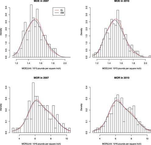
Figure 1: Histograms of MOE and MOR with EL and EM density estimates.

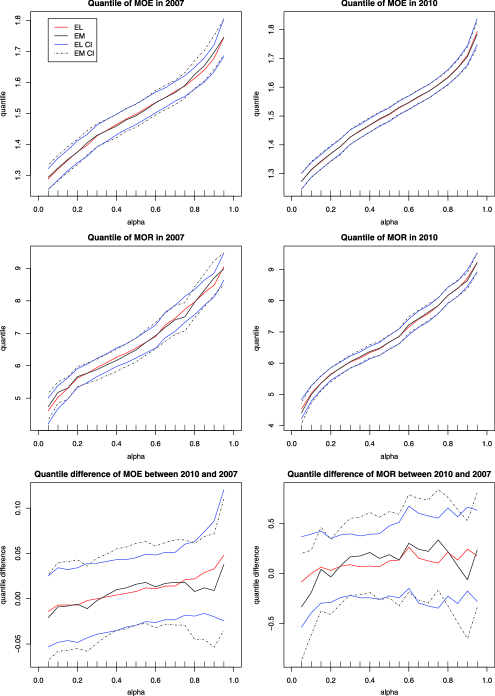
Figure 2: Point estimates and confidence intervals for quantiles and quantile differences for lumber data.

Appendix

.1 Sketched proof of Theorem 2.1

This theorem mostly summarizes and extends the results in Qin and Zhang (1997), Fokianos et al. (2001) and Zhang (2002). To enable readers to understand the other proofs, we provide some necessary details. Interested readers can contact the authors for more detailed derivations.

Lemma .1

Assume the conditions of Theorem 2.1. For any $\bolds{\theta}$ such that $\bolds{\theta}=\bolds{\theta}^{*}+o(n^{-1/3})$, we have

$$\ell_{n}(\bolds{\theta})-\ell_{n}\bigl{(}\bolds{\theta}^{*}\bigr{)}=\bigl{(}\bolds{\theta}-\bolds{\theta}^{*}\bigr{)}^{\tau}\mathbf{Z}_{n}-\frac{n}{2}\bigl{(}\bolds{\theta}-\bolds{\theta}^{*}\bigr{)}^{\tau}\mathbf{W}\bigl{(}\bolds{\theta}-\bolds{\theta}^{*}\bigr{)}+o_{p}(1),$$

where the vector $\mathbf{Z}_{n}$ is

$$\mathbf{Z}_{n,r} = \sum_{j=1}^{n_{r}}\mathbf{q}(x_{rj})-\sum_{k,j}h_{r}(x_{kj})\mathbf{q}(x_{kj})$$

$$= \sum_{k,j}\bigl{[}\bigl{\{}\delta_{kr}-h_{r}(x_{kj})\bigr{\}}\mathbf{q}(x_{kj})\bigr{]},$$

and $n^{-1/2}\mathbf{Z}_{n}$ is asymptotic normal with mean $\mathbf{0}$ and a positive definite covariance matrix.

Note that $\mathbf{Z}_{n}$ is a sum of independent random vectors with finite moments. The mean of each is not zero, but the total is zero. In Theorem 3.2 we defined the $r$th segment of $\mathbf{B}_{k}=\mathbf{B}_{k}(\infty)$ as

$$\mathbf{B}_{k,r} = {\rho_{k}}\mathsf{E}\bigl{\{}\delta_{kr}\mathbf{q}(x_{kj})-h_{r}(x_{kj})\mathbf{q}(x_{kj})\bigr{\}}$$

$$= \int\bigl{\{}\delta_{kr}h_{k}(x)-h_{r}(x)h_{k}(x)\bigr{\}}\mathbf{q}(x)\,d\bar{G}(x).$$

An interesting and useful observation is that for $1\leq k,r\leq m$, $\mathbf{B}_{k,r}=\mathbf{B}_{r,k}$. From $\sum_{k=0}^{m}h_{k}(x)=1$, we may also verify that

$$\mathsf{E}\{Z_{n,r}\}=n\sum_{k=0}^{m}\mathbf{B}_{k,r}=0.$$

Thus, $n^{-1/2}\mathbf{Z}_{n}$ is asymptotic normal with mean $\mathbf{0}$ and some variance matrix. This fact together with the form of the quadratic approximation implies that $\ell_{n}(\bolds{\theta})-\ell_{n}(\bolds{\theta}^{*})$ is maximized at the $\hat{\bolds{\theta}}$ that satisfies

$$n^{1/2}\bigl{(}\hat{\bolds{\theta}}-\bolds{\theta}^{*}\bigr{)}=n^{-1/2}\mathbf{W}^{-1}\mathbf{Z}_{n}+o_{p}(1).$$

See Hjort and Pollard (1993) for this justification.

The remaining task is to verify that the asymptotic variance of $n^{-1/2}\mathbf{Z}_{n}$ is given by $\mathbf{W}-\mathbf{W}\mathbf{S}\mathbf{W}$. This proves Theorem 2.1.

.2 Proof of Theorem 3.1

The key to the proof is to show a seemingly obvious claim: $\hat{\xi}_{r}-\xi_{r}=O_{p}(n^{-1/2}).$ This is an immediate consequence of

$$\hat{G}_{r}(x)-G_{r}(x)=O_{p}\bigl{(}n^{-1/2}\bigr{)}$$ (11)

uniformly for $x$ in a neighborhood of $\xi_{r}$. We now prove (11). Recall that

$$\hat{G}_{r}(x)=n_{r}^{-1}\sum_{k,j}h_{r}(x_{kj};\hat{\bolds{\theta}})I(x_{kj}\leq x).$$

Replacing $\hat{\bolds{\theta}}$ in $\hat{G}_{r}(x)$ by its true value $\bolds{\theta}^{*}$, we define

$$\tilde{G}_{r}(x)=n_{r}^{-1}\sum_{k,j}{h_{r}\bigl{(}x_{kj};\bolds{\theta}^{*}\bigr{)}}I(x_{kj}\leq x),$$

a sum of independent random variables. From $\mathsf{E}\{\tilde{G}_{r}(x)\}=G_{r}(x)$, we get

$$\mathsf{E}\bigl{\{}\tilde{G}_{r}(x)-G_{r}(x)\bigr{\}}^{2}=n_{r}^{-2}\sum_{k,j}\operatorname{var}\bigl{\{}{h_{r}\bigl{(}x_{kj};\bolds{\theta}^{*}\bigr{)}}I(x_{kj}\leq x)\bigr{\}}.$$

Since $0\leq h_{r}(x;\bolds{\theta}^{*})\leq 1$, we have $\operatorname{var}\{h_{r}(x_{kj};\bolds{\theta}^{*})I(x_{kj}\leq x)\}\leq 1$. Hence,

$$\sup_{x}\mathsf{E}\bigl{\{}G_{r}(x)-\tilde{G}_{r}(x)\bigr{\}}^{2}\leq n/n_{r}^{2}=O\bigl{(}n^{-1}\bigr{)}.$$

Since $G_{r}(x)$ and $\tilde{G}_{r}(x)$ are distribution functions, the above rate is uniform in $x$. Hence

$$\sup_{x}\bigl{|}\tilde{G}_{r}(x)-G_{r}(x)\bigr{|}=O_{p}\bigl{(}n^{-1/2}\bigr{)}.$$

Therefore, (11) is implied by $\sup_{x}|\hat{G}_{r}(x)-\tilde{G}_{r}(x)|=O_{p}(n^{-1/2})$. Note that

$$\tilde{G}_{r}(x)-\hat{G}_{r}(x) = n_{r}^{-1}\sum_{k,j}\bigl{\{}{h_{r}\bigl{(}x_{kj};\bolds{\theta}^{*}\bigr{)}}-h_{r}(x_{kj};\hat{\bolds{\theta}})\bigr{\}}I(x_{kj}\leq x).$$

The partial derivative of $h_{r}(x;\bolds{\theta})$ with respect to $\bolds{\theta}$ is bounded by $\sqrt{m}\|\mathbf{q}(x)\|$. Thus

$$\bigl{|}\tilde{G}_{r}(x)-\hat{G}_{r}(x)\bigr{|}\leq(n\rho_{r})^{-1}\bigl{\|}\hat{\bolds{\theta}}-\bolds{\theta}^{*}\bigr{\|}\sum_{k,j}\sqrt{m}\bigl{\|}\mathbf{q}(x_{kj})\bigr{\|}.$$

The conditions of Theorem 2.1 imply that $\mathbf{q}(x_{kj})$ has finite moments of any order. Thus, $n^{-1}\sum_{k,j}\|\mathbf{q}(x_{kj})\|=O_{p}(1),$ and subsequently,

$$\bigl{|}\tilde{G}_{r}(x)-\hat{G}_{r}(x)\bigr{|} \leq (n\rho_{r})^{-1}\bigl{\|}\hat{\bolds{\theta}}-\bolds{\theta}^{*}\bigr{\|}\sum_{k,j}\sqrt{m}\bigl{\|}\mathbf{q}(x_{kj})\bigr{\|}=O_{p}\bigl{(}\bigl{\|}\hat{\bolds{\theta}}-\bolds{\theta}^{*}\bigr{\|}\bigr{)}$$

$$= O_{p}\bigl{(}n^{-1/2}\bigr{)}.$$

This completes the proof of (11).

The classical Bahadur representation was a rate result in the mode of “almost sure.” Our result is stated in terms of “in probability,” and therefore it has a simpler proof. As for the classical case, the representation is equivalent to the following lemma:

Lemma .2

Under the conditions of Theorem 3.1, for any $c>0$ and $r=0,1,\ldots,m$, we have

$$\sup_{x\dvtx|x-\xi_{r}|<cn^{-1/2}}\bigl{|}\bigl{\{}\hat{G}_{r}(x)-\hat{G}_{r}(\xi_{r})\bigr{\}}-\bigl{\{}G_{r}(x)-G_{r}(\xi_{r})\bigr{\}}\bigr{|}=O_{p}\bigl{(}n^{-3/4}\bigl{(}\log(n)\bigr{)}^{1/2}\bigr{)}.$$

We prove this lemma for $r=0$; the other cases are equivalent. Without loss of generality we assume $x\geq\xi_{r}$. Note that

$$\bigl{\{}\hat{G}_{0}(x)-\hat{G}_{0}(\xi_{r})\bigr{\}}-\bigl{\{}\tilde{G}_{0}(x)-\tilde{G}_{0}(\xi_{r})\bigr{\}}$$

$$\qquad=n_{0}^{-1}\sum_{k,j}\bigl{\{}h_{0}(x_{kj};\hat{\bolds{\theta}})-h_{0}\bigl{(}x_{kj};\bolds{\theta}^{*}\bigr{)}\bigr{\}}I(\xi_{r}<x_{kj}\leq x).$$

By the mean value theorem and the specific form of $h_{0}(x;\bolds{\theta})$, we have

$$\bigl{|}h_{0}(x_{kj};\hat{\bolds{\theta}})-h_{0}\bigl{(}x_{kj};\bolds{\theta}^{*}\bigr{)}\bigr{|}\leq\sqrt{m}\bigl{\|}\mathbf{q}(x_{kj})\bigr{\|}\bigl{\|}\hat{\bolds{\theta}}-\bolds{\theta}^{*}\bigr{\|}.$$

From $\mathsf{E}\{\|\mathbf{q}(x_{kj})\|\}<\infty$, we get $\mathsf{E}\{\mathbf{q}(x_{kj})I(\xi_{r}<x_{kj}\leq x)\}=O(n^{-1/2})$ and

$$\bigl{\{}\hat{G}_{0}(x)-\hat{G}_{0}(\xi_{r})\bigr{\}}-\bigl{\{}\tilde{G}_{0}(x)-\tilde{G}_{0}(\xi_{r})\bigr{\}}=O_{p}\bigl{(}n^{-1}\bigr{)}.$$

With this result, Lemma .2 is proved if we show that

$$\sup_{x\dvtx|x-\xi|<cn^{-1/2}}\bigl{|}\bigl{[}\tilde{G}_{0}(x)-\tilde{G}_{0}(\xi_{r})\bigr{]}-\bigl{[}G_{0}(x)-G_{0}(\xi_{r})\bigr{]}\bigr{|}=O_{p}\bigl{(}n^{-3/4}\bigl{(}\log(n)\bigr{)}^{1/2}\bigr{)}.$$

Since $\tilde{G}_{0}(x)$ is a sum of bounded random variables and $\mathsf{E}\{\tilde{G}_{0}(x)\}=G_{0}(x)$, the result can be proved following Lemma 2.5.4E in Serfling (1980), page 97; we omit the details here. This completes the proof.

Proof of Theorem 3.1 We have $\hat{\xi}_{r}-\xi_{r}=O_{p}(n^{-1/2})$ for any $\xi_{r}$, and the derivative of $G_{r}$ is positive and continuous in a neighborhood of $\xi_{r}$. Therefore,

$$G_{r}(\hat{\xi}_{r})-G_{r}(\xi_{r})=g_{r}(\xi_{r})(\hat{\xi}_{r}-\xi_{r})+O_{p}\bigl{(}n^{-1}\bigr{)}.$$

By definition, we have $\hat{G}_{r}(\hat{\xi}_{r})=\alpha_{r}+O(n^{-1})$. Thus, replacing $x$ by $\hat{\xi}_{r}$, and $\xi$ by $\xi_{r}$, the result of Lemma .2 becomes

$$\bigl{|}\bigl{\{}\alpha-\hat{G}_{r}(\xi_{r})\bigr{\}}-g_{r}(\xi_{r})(\hat{\xi}_{r}-\xi_{r})\bigr{|}=O_{p}\bigl{(}n^{-3/4}\bigl{(}\log(n)\bigr{)}^{1/2}\bigr{)}.$$

This is equivalent to the conclusion of the theorem.

.3 Proof of Theorem 3.2

Theorem 3.2 characterizes the asymptotic joint normality of a number of MELE distribution estimates. It is proved by approximating $\hat{G}_{r}(x)$ by a summation of independent random variables.

By the proof of Theorem 2.1, $\hat{\bolds{\theta}}-\bolds{\theta}^{*}=n^{-1}\mathbf{W}^{-1}\mathbf{Z}_{n}+o_{p}(1).$ Hence,

$$\hat{G}_{r}(x) = n_{r}^{-1}\sum_{k,j}h_{r}(x_{kj};\hat{\bolds{\theta}})I(x_{kj}\leq x)$$

$$= n_{r}^{-1}\sum_{k,j}\bigl{[}h_{r}(x_{kj})+\bigl{\{}\dot{h}_{r}\bigl{(}x_{kj};\bolds{\theta}^{*}\bigr{)}\bigr{\}}^{\tau}\bigl{(}\hat{\bolds{\theta}}-\bolds{\theta}^{*}\bigr{)}\bigr{]}I(x_{kj}\leq x)+o_{p}\bigl{(}n^{-{1}/{2}}\bigr{)}$$

$$= n_{r}^{-1}\sum_{k,j}h_{r}(x_{kj})I(x_{kj}\leq x)$$

$${}+n_{r}^{-1}\biggl{\{}n^{-1}\sum_{k,j}\dot{h}_{r}\bigl{(}x_{kj};\bolds{\theta}^{*}\bigr{)}I(x_{kj}<x)\biggr{\}}^{\tau}\mathbf{W}^{-1}\mathbf{Z}_{n}+o_{p}\bigl{(}n^{-{1}/{2}}\bigr{)},$$

where $\dot{h}_{r}(x;\bolds{\theta}^{*})={\partial h_{r}(x;\bolds{\theta})}/{\partial\bolds{\theta}}|_{\bolds{\theta}=\bolds{\theta}^{*}}$. Working out the expression of $\dot{h}_{r}(x;\bolds{\theta}^{*})$ in terms of $\mathbf{q}(x)$ and $h_{r}(x)$, and by the law of large numbers, we find that, almost surely,

$$n^{-1}\sum_{k,j}\dot{h}_{r}\bigl{(}x_{kj};\bolds{\theta}^{*}\bigr{)}I(x_{kj}<x)\to\mathbf{B}_{r}(x),$$

where $\mathbf{B}_{r}(x)$ is defined in the theorem. We remark here that $\lim_{x\to\infty}\mathbf{B}_{r}(x)=\mathbf{B}_{r}$; the latter was defined in the proof of Theorem 2.1. Before the final step, we may verify that

$$G_{r}(x)=n_{r}^{-1}{\mathsf{E}}\biggl{\{}\sum_{k,j}h_{r}(x_{kj})I(x_{kj}\leq x)\biggr{\}}.$$

These preparations enable us to write

$$\hat{G}_{r}(x)-G_{r}(x) = n_{r}^{-1}\sum_{k,j}\bigl{[}h_{r}(x_{kj})I(x_{kj}\leq x)-\mathsf{E}\bigl{\{}h_{r}(x_{kj})I(x_{kj}\leq x)\bigr{\}}\bigr{]}$$

$${}+n_{r}^{-1}\mathbf{B}_{r}^{\tau}(x)\mathbf{W}^{-1}\mathbf{Z}_{n}+o_{p}\bigl{(}n^{1/2}\bigr{)}.$$

The two leading terms are summations of independent random vectors and both have mean zero. The joint asymptotic normality of $\sqrt{n}\{\hat{G}_{r}(x)-G_{r}(x)\}$ and $\sqrt{n}\{\hat{G}_{s}(y)-G_{s}(y)\}$ is hence implied. We derive the algebraic expression of $\omega_{rs}(x,y)$ in the next subsection.

.3.1 Asymptotic covariance $\sigma_{rs}(x,y)$

From the expansion of $\hat{G}_{r}(x)-G_{r}(x)$, $\omega_{rs}(x,y)$ is decomposed into four covariances. Using $\operatorname{var}(\mathbf{Z}_{n})=n(\mathbf{W}-\mathbf{W}\mathbf{S}\mathbf{W})$ as shown earlier, we find that one of them is given by

$$\operatorname{Cov}\bigl{(}\mathbf{B}_{r}^{\tau}(x)\mathbf{W}^{-1}\mathbf{Z}_{n},\mathbf{B}_{s}^{\tau}(y)\mathbf{W}^{-1}\mathbf{Z}_{n}\bigr{)}=n\mathbf{B}_{r}^{\tau}(x)\bigl{(}\mathbf{W}^{-1}-\mathbf{S}\bigr{)}\mathbf{B}_{s}(y).$$

We build another term from the following computations:

$$\operatorname{Cov}\bigl{\{}h_{r}(x_{kj})I(x_{kj}\leq x),h_{s}(x_{kj})I(x_{kj}\leq y)\bigr{\}}$$

$$\qquad=\rho_{k}^{-1}\int_{-\infty}^{(x\wedge y)}h_{r}(x)h_{s}(x)h_{k}(x)\,d\bar{G}(x)-\rho_{k}^{-2}c_{rk}(x)c_{sk}(y),$$

where $c_{rs}(x)=\int_{-\infty}^{x}h_{r}(t)h_{s}(t)\,d\bar{G}(t)$. Because $\sum_{k=0}^{m}h_{k}(x)=1$, we get

$$\sum_{k=0}^{m}n_{k}\operatorname{Cov}\bigl{\{}h_{r}(x_{kj})I(x_{kj}\leq x),h_{s}(x_{kj})I(x_{kj}\leq y)\bigr{\}}$$

$$\qquad=n\Biggl{\{}c_{rs}(x\wedge y)-\sum_{k=0}^{m}\rho_{k}^{-1}c_{rk}(x)c_{sk}(y)\Biggr{\}}.$$

The last task is the cross-term $\operatorname{Cov}\{h_{r}(x_{kj})I(x_{kj}\leq x),\mathbf{Z}_{n}\}$. We break $\mathbf{Z}_{n}$ into segments $\mathbf{Z}_{n,s}$ and then into centralized $\tilde{\mathbf{Z}}_{n,s}$.

$$\operatorname{Cov}\bigl{\{}h_{r}(x_{kj})I(x_{kj}\leq x),\mathbf{Z}_{n,s}\bigr{\}}$$

$$\qquad=\mathsf{E}\bigl{[}h_{r}(x_{kj})I(x_{kj}\leq x)\bigl{\{}{\bigl{(}\delta_{kr}-h_{s}(x_{kj})\bigr{)}}\mathbf{q}^{\tau}(x_{kj})-\rho_{k}^{-1}\mathbf{B}_{k,s}^{\tau}\bigr{\}}\bigr{]}$$

$$\qquad=\rho_{k}^{-1}{\mathbf{B}^{\tau}_{k,r}(x)}-\rho_{k}^{-2}c_{rk}(x){\mathbf{B}^{\tau}_{k,s}}.$$

Summing over $\{k,j\}$, the first term sums to zero, so we find

$$\operatorname{Cov}\biggl{\{}\sum_{k,j}h_{r}(x_{kj})I(x_{kj}\leq x),\mathbf{Z}_{n,s}\biggr{\}}=-n\sum_{k=0}^{m}\rho_{k}^{-1}c_{rk}(x){\mathbf{B}^{\tau}_{k,s}}.$$

Next, we assemble $\mathbf{B}_{k,s}$ over $s$ to get $\mathbf{B}_{k}$,

$$\operatorname{Cov}\biggl{\{}\sum_{k,j}h_{r}(x_{kj})I(x_{kj}\leq x),\mathbf{Z}_{n}\biggr{\}}=-n\sum_{k=0}^{m}\rho_{k}^{-1}c_{rk}(x){\mathbf{B}^{\tau}_{k}}.$$

Entering $\mathbf{B}_{s}^{\tau}(y)\mathbf{W}^{-1}$ into the second argument of the covariance, we get

$$\operatorname{Cov}\biggl{\{}\sum_{k,j}h_{r}(x_{kj})I(x_{kj}\leq x),{\mathbf{B}_{s}^{\tau}(y)}\mathbf{W}^{-1}\mathbf{Z}_{n}\!\biggr{\}}=-n\sum_{k=0}^{m}\rho_{k}^{-1}c_{rk}(x)\mathbf{B}_{k}^{\tau}\mathbf{W}^{-1}\mathbf{B}_{s}(y).$$

Thus, the covariance between $\sqrt{n}\{\hat{G}_{r}(x)-G_{r}(x)\}$ and $\sqrt{n}\{\hat{G}_{s}(y)-G_{s}(y)\}$ is given by

$$\omega_{rs}(x,y) = (\rho_{r}\rho_{s})^{-1}\Biggl{[}c_{rs}(x\wedge y)-\sum_{k=0}^{m}\rho_{k}^{-1}c_{rk}(x)c_{sk}(y)$$

$$\hskip 43.0pt{}-\sum_{k=0}^{m}\rho_{k}^{-1}\mathbf{B}_{k}^{\tau}\mathbf{W}^{-1}\bigl{\{}{c_{rk}(x)\mathbf{B}_{s}(y)+c_{sk}(y)\mathbf{B}_{r}(x)}\bigr{\}}$$

$$\hskip 117.0pt\qquad{}+\mathbf{B}_{r}^{\tau}(x)\bigl{(}\mathbf{W}^{-1}-\mathbf{S}\bigr{)}\mathbf{B}_{s}(y)\Biggr{]}.$$

Further simplification is possible. We find $c_{r0}(x)+\mathbf{B}_{r}^{\tau}(x)\mathbf{W}^{-1}\mathbf{B}_{0}=0$, $c_{rk}(x)+\mathbf{B}_{r}^{\tau}(x)\mathbf{W}^{-1}\mathbf{B}_{k}=\delta_{rk}G_{r}(x)$ and $\sum_{k=0}^{m}\rho_{k}^{-1}\mathbf{W}^{-1}\mathbf{B}_{k}\mathbf{B}_{k}^{\tau}\mathbf{W}^{-1}=\mathbf{S}$. These findings lead to

$$\omega_{rs}(x,y)=(\rho_{r}\rho_{s})^{-1}\bigl{\{}c_{rs}(x\wedge y)+\mathbf{B}_{r}^{\tau}(x)\mathbf{W}^{-1}\mathbf{B}_{s}(y)-\rho_{r}\delta_{rs}G_{r}(x)G_{s}(y)\bigr{\}}.$$

The final expression (8) is obtained by noticing that $c_{rs}(x)=\rho_{r}\delta_{rs}G_{r}(x)-a_{rs}(x),$ where $a_{rs}(x)$ was defined in Theorem 3.2.

.4 Proof of Theorem 4.1

Both the EL and EM quantiles admit Bahadur representations, and it suffices to show the same conclusion for the distribution estimators. For the bivariate case, we denote the asymptotic covariance matrices of the EL and EM distributions as

$$\Omega_{\operatorname{EL}}=\pmatrix{\sigma_{rr}(x,x)&\sigma_{rs}(x,y)\vspace*{2pt}\cr\sigma_{rs}(x,y)&\sigma_{ss}(y,y)},\qquad\Omega_{\operatorname{EM}}=\pmatrix{\omega_{rr}(x,x)&\omega_{rs}(x,y)\vspace*{2pt}\cr\omega_{rs}(x,y)&\omega_{ss}(y,y)},$$

where $x=\xi_{r}$ and $y=\xi_{s}$ are two population quantiles or two real values. We show that $\Omega_{\operatorname{EM}}-\Omega_{\operatorname{EL}}$ is nonnegative definite by writing it as $D_{11}-D_{12}D_{22}^{-1}D_{21}$, with the $D_{ij}$ being blocks of a nonnegative definite matrix $D$. By standard matrix theory, the nonnegative definiteness of $D$ implies that of $D_{11}-D_{12}D_{22}^{-1}D_{21}$. The generic element of $\Omega_{\operatorname{EM}}-\Omega_{\operatorname{EL}}$ is $a_{rs}(x,y)-\mathbf{B}_{r}^{\tau}(x)\mathbf{W}^{-1}\mathbf{B}_{s}(y),$ which fits into $D_{11}-D_{12}D_{22}^{-1}D_{21}$ with

$$D_{11}=\pmatrix{a_{rr}(x)&a_{rs}(x\wedge y)\vspace*{2pt}\cr a_{rs}(x\wedge y)&a_{ss}(y)},\qquad D_{12}=\pmatrix{\mathbf{B}_{r}^{\tau}(x)\vspace*{2pt}\cr\mathbf{B}_{s}^{\tau}(y)},$$

$D_{21}=D_{12}^{\tau}$ and $D_{22}=\mathbf{W}$. We will show that $D=\int\mathbf{U}(z)\,d\bar{G}(z)$ for some nonnegative definite $\mathbf{U}(z)$ for all $z$. Then $D$ is nonnegative definite and so is $\Omega_{\operatorname{EM}}-\Omega_{\operatorname{EL}}=D_{11}-D_{12}D_{22}^{-1}D_{21}.$

We now search for such a $\mathbf{U}(z)$. We write

$$a_{rs}(x\wedge y) = \int I(z\leq x)I(z\leq y)\mathbf{H}[r+1,s+1](z)\,d\bar{G}(z),$$

$$\mathbf{B}_{r}(x) = \int I(z\leq x)\mathbf{H}[-1,r+1](z)\otimes\mathbf{q}(z)\,d\bar{G}(z),$$

$$\mathbf{W} = \int\mathbf{H}[-1,-1](z)\otimes\bigl{\{}\mathbf{q}(z)\mathbf{q}^{\tau}(z)\bigr{\}}\,d\bar{G}(z).$$

Using the Khatrin–Rao product operator $\ast$ [Liu and Trenkler (2008)], we find such a $\mathbf{U}(z)=A_{1}(z)\ast A_{2}(z)$ with

$$A_{1}(z) = P\pmatrix{\mathbf{H}[r+1,r+1](z)&\mathbf{H}[r+1,s+1](z)&\mathbf{H}[r+1,-1](z)\vspace*{2pt}\cr\mathbf{H}[s+1,r+1](z)&\mathbf{H}[s+1,s+1](z)&\mathbf{H}[s+1,-1](z)\vspace*{2pt}\cr\mathbf{H}[-1,r+1](z)&\mathbf{H}[-1,s+1](z)&\mathbf{H}[-1,-1](z)}P,$$

$$A_{2}(z) = \pmatrix{1&1&\mathbf{q}^{\tau}(z)\vspace*{2pt}\cr 1&1&\mathbf{q}^{\tau}(z)\vspace*{2pt}\cr\mathbf{q}(z)&\mathbf{q}(z)&\mathbf{q}(z)\mathbf{q}^{\tau}(z)},\qquad P=\pmatrix{I(z\leq x)&0&0\vspace*{2pt}\cr 0&I(z\leq y)&0\vspace*{2pt}\cr 0&0&\mathbf{I}_{m}}.$$

The matrix $A_{2}(z)$ is clearly nonnegative definite for any $z$. Note that $\mathbf{H}(z)$ is nonnegative definite for any $z$; the nonnegative definiteness of $A_{1}(z)$ is an easy consequence. Since the $\ast$ product of two nonnegative definite matrices is still nonnegative definite [Lemma 5 of Liu and Trenkler (2008)], we conclude that $\mathbf{U}(z)=A_{1}(z)\ast A_{2}(z)$ is also nonnegative definite for any $z$. This completes the proof. This proof can easily be extended to the case where more distributions or quantiles are involved.

References

• Anderson (1979) {barticle}[mr] \bauthor\bsnmAnderson, \bfnmJ. A.\binitsJ. A. (\byear1979). \btitleMultivariate logistic compounds. \bjournalBiometrika \bvolume66 \bpages17–26. \biddoi=10.1093/biomet/66.1.17, issn=0006-3444, mr=0529143 \bptokimsref \endbibitem
• Bahadur (1966) {barticle}[mr] \bauthor\bsnmBahadur, \bfnmR. R.\binitsR. R. (\byear1966). \btitleA note on quantiles in large samples. \bjournalAnn. Math. Statist. \bvolume37 \bpages577–580. \bidissn=0003-4851, mr=0189095 \bptokimsref \endbibitem
• Chen and Chen (2000) {barticle}[mr] \bauthor\bsnmChen, \bfnmHanfeng\binitsH. and \bauthor\bsnmChen, \bfnmJiahua\binitsJ. (\byear2000). \btitleBahadur representations of the empirical likelihood quantile processes. \bjournalJ. Nonparametr. Stat. \bvolume12 \bpages645–660. \biddoi=10.1080/10485250008832826, issn=1048-5252, mr=1784802 \bptokimsref \endbibitem
• Deheuvels (1977) {barticle}[mr] \bauthor\bsnmDeheuvels, \bfnmPaul\binitsP. (\byear1977). \btitleEstimation non paramétrique de la densité par histogrammes généralisés. \bjournalRev. Statist. Appl. \bvolume25 \bpages5–42. \bidissn=0035-175X, mr=0501555 \bptokimsref \endbibitem
• Fokianos (2007) {barticle}[mr] \bauthor\bsnmFokianos, \bfnmKonstantinos\binitsK. (\byear2007). \btitleDensity ratio model selection. \bjournalJ. Stat. Comput. Simul. \bvolume77 \bpages805–819. \biddoi=10.1080/10629360600673857, issn=0094-9655, mr=2409865 \bptokimsref \endbibitem
• Fokianos and Kaimi (2006) {barticle}[mr] \bauthor\bsnmFokianos, \bfnmKonstantinos\binitsK. and \bauthor\bsnmKaimi, \bfnmIrene\binitsI. (\byear2006). \btitleOn the effect of misspecifying the density ratio model. \bjournalAnn. Inst. Statist. Math. \bvolume58 \bpages475–497. \biddoi=10.1007/s10463-005-0022-8, issn=0020-3157, mr=2327888 \bptokimsref \endbibitem
• Fokianos et al. (2001) {barticle}[mr] \bauthor\bsnmFokianos, \bfnmKonstantinos\binitsK., \bauthor\bsnmKedem, \bfnmBenjamin\binitsB., \bauthor\bsnmQin, \bfnmJing\binitsJ. and \bauthor\bsnmShort, \bfnmDavid A.\binitsD. A. (\byear2001). \btitleA semiparametric approach to the one-way layout. \bjournalTechnometrics \bvolume43 \bpages56–65. \biddoi=10.1198/00401700152404327, issn=0040-1706, mr=1819908 \bptokimsref \endbibitem
• Hjort and Pollard (1993) {bmisc}[auto:STB—2013/06/05—13:45:01] \bauthor\bsnmHjort, \bfnmN. L.\binitsN. L. and \bauthor\bsnmPollard, \bfnmD.\binitsD. (\byear1993). \bhowpublishedAsymptotics for minimisers of convex processes. Technical report, Yale Univ. \bptokimsref \endbibitem
• Keziou and Leoni-Aubin (2008) {barticle}[mr] \bauthor\bsnmKeziou, \bfnmAmor\binitsA. and \bauthor\bsnmLeoni-Aubin, \bfnmSamuela\binitsS. (\byear2008). \btitleOn empirical likelihood for semiparametric two-sample density ratio models. \bjournalJ. Statist. Plann. Inference \bvolume138 \bpages915–928. \biddoi=10.1016/j.jspi.2007.02.009, issn=0378-3758, mr=2384498 \bptokimsref \endbibitem
• Kiefer (1967) {barticle}[mr] \bauthor\bsnmKiefer, \bfnmJ.\binitsJ. (\byear1967). \btitleOn Bahadur’s representation of sample quantiles. \bjournalAnn. Math. Statist. \bvolume38 \bpages1323–1342. \bidissn=0003-4851, mr=0217844 \bptokimsref \endbibitem
• Liu and Trenkler (2008) {barticle}[mr] \bauthor\bsnmLiu, \bfnmShuangzhe\binitsS. and \bauthor\bsnmTrenkler, \bfnmGötz\binitsG. (\byear2008). \btitleHadamard, Khatri–Rao, Kronecker and other matrix products. \bjournalInt. J. Inf. Syst. Sci. \bvolume4 \bpages160–177. \bidissn=1708-296X, mr=2401772 \bptokimsref \endbibitem
• Owen (1988) {barticle}[mr] \bauthor\bsnmOwen, \bfnmArt B.\binitsA. B. (\byear1988). \btitleEmpirical likelihood ratio confidence intervals for a single functional. \bjournalBiometrika \bvolume75 \bpages237–249. \biddoi=10.1093/biomet/75.2.237, issn=0006-3444, mr=0946049 \bptokimsref \endbibitem
• Owen (2001) {bbook}[auto:STB—2013/06/05—13:45:01] \bauthor\bsnmOwen, \bfnmA. B.\binitsA. B. (\byear2001). \btitleEmpirical Likelihood. \bpublisherChapman & Hall/CRC, \blocationNew York. \bptokimsref \endbibitem
• Qin and Zhang (1997) {barticle}[mr] \bauthor\bsnmQin, \bfnmJing\binitsJ. and \bauthor\bsnmZhang, \bfnmBiao\binitsB. (\byear1997). \btitleA goodness-of-fit test for logistic regression models based on case–control data. \bjournalBiometrika \bvolume84 \bpages609–618. \biddoi=10.1093/biomet/84.3.609, issn=0006-3444, mr=1603924 \bptokimsref \endbibitem
• R Development Core Team (2011) {bmisc}[auto:STB—2013/06/05—13:45:01] \borganizationR Development Core Team (\byear2011). \bhowpublishedR: A Language and Environment for Statistical Computing. R Foundation for Statistical Computing, Vienna, Austria. \bptokimsref \endbibitem
• Serfling (1980) {bbook}[mr] \bauthor\bsnmSerfling, \bfnmRobert J.\binitsR. J. (\byear1980). \btitleApproximation Theorems of Mathematical Statistics. \bpublisherWiley, \blocationNew York. \bidmr=0595165 \bptokimsref \endbibitem
• Silverman (1986) {bbook}[mr] \bauthor\bsnmSilverman, \bfnmB. W.\binitsB. W. (\byear1986). \btitleDensity Estimation for Statistics and Data Analysis. \bpublisherChapman & Hall, \blocationLondon. \bidmr=0848134 \bptokimsref \endbibitem
• Wu (2005) {barticle}[mr] \bauthor\bsnmWu, \bfnmWei Biao\binitsW. B. (\byear2005). \btitleOn the Bahadur representation of sample quantiles for dependent sequences. \bjournalAnn. Statist. \bvolume33 \bpages1934–1963. \biddoi=10.1214/009053605000000291, issn=0090-5364, mr=2166566 \bptokimsref \endbibitem
• Zhang (2000) {barticle}[mr] \bauthor\bsnmZhang, \bfnmBiao\binitsB. (\byear2000). \btitleQuantile estimation under a two-sample semi-parametric model. \bjournalBernoulli \bvolume6 \bpages491–511. \biddoi=10.2307/3318672, issn=1350-7265, mr=1762557 \bptokimsref \endbibitem
• Zhang (2002) {barticle}[mr] \bauthor\bsnmZhang, \bfnmBiao\binitsB. (\byear2002). \btitleAssessing goodness-of-fit of generalized logit models based on case-control data. \bjournalJ. Multivariate Anal. \bvolume82 \bpages17–38. \biddoi=10.1006/jmva.2001.2019, issn=0047-259X, mr=1918613 \bptokimsref \endbibitem
• Zhou and Wu (2009) {barticle}[mr] \bauthor\bsnmZhou, \bfnmZhou\binitsZ. and \bauthor\bsnmWu, \bfnmWei Biao\binitsW. B. (\byear2009). \btitleLocal linear quantile estimation for nonstationary time series. \bjournalAnn. Statist. \bvolume37 \bpages2696–2729. \biddoi=10.1214/08-AOS636, issn=0090-5364, mr=2541444 \bptokimsref \endbibitem