Regressions with Berkson errors in covariates—A nonparametric approach

Abstract

This paper establishes that so-called instrumental variables enable the identification and the estimation of a fully nonparametric regression model with Berkson-type measurement error in the regressors. An estimator is proposed and proven to be consistent. Its practical performance and feasibility are investigated via Monte Carlo simulations as well as through an epidemiological application investigating the effect of particulate air pollution on respiratory health. These examples illustrate that Berkson errors can clearly not be neglected in nonlinear regression models and that the proposed method represents an effective remedy.

t1Supported in part by NSF Grants SES-0752699 and SES-1156347, and through TeraGrid computer resources provided by the University of Texas under Grant SES-070003.

1 Introduction

Many statistical data sets involve covariates $X$ that are error-contaminated versions of their true unobserved counterpart $X^{\ast}$. However, the measurement error often does not fit the classical error structure $X=X^{\ast}+\Delta X$ with $\Delta X$ independent from $X^{\ast}$. A common occurrence is, in fact, the opposite situation, in which $X^{\ast}=X+\Delta X^{\ast}$ with $\Delta X^{\ast}$ independent from $X$, a situation often referred to as Berkson measurement error [Berkson (1950), Wang (2004), Carroll et al. (2006)]. A typical example is an epidemiological study in which an individual’s true exposure $X^{\ast}$ to some contaminant is not observed, but instead, what is available is the average concentration $X$ of this contaminant in the region where the individual lives. The individual-specific $X^{\ast}$ randomly fluctuate around the region average $X$, resulting in Berkson errors.

Existing approaches to handle data with Berkson measurement error [e.g., Delaigle, Hall and Qiu (2006), Carroll, Delaigle and Hall (2007)] unfortunately require the distribution of the measurement error to be known, or to be estimated via validation data, which can be costly, difficult or impossible to collect. (In classical measurement error problems, the distribution of the error can be identified from repeated measurements via a Kotlarski-type equality [Schennach (2004), Li and Vuong (1998)]. However, such results do not yet exist for Berkson-type measurement error.) A popular approach to relax the assumption of a fully known distribution of the measurement error is to allow for some adjustable parameters in the distributions of the variables and their relationships, and solve for the parameter values that best reproduce various conditional moments of the observed variables, under the assumption that this solution is unique. This approach has been used, in particular, for polynomial specifications [Huwang and Huang (2000)] and, more recently, for a very wide range of parametric models [Wang (2004, 2007)].

The present paper goes beyond this and provides a formal identification result and a general nonparametric regression method that is consistent in the presence of Berkson errors, without requiring the distribution of the measurement error to be known a priori. Instead, the method relies on the availability of a so-called instrumental variable [e.g., see Chapter 6 in Carroll et al. (2006)] to recover the relationship of interest. For instance, in the epidemiological study of the effect of particulate matter pollution on respiratory health we consider in this paper, suitable instruments could include (i) individual-level measurement of contaminant levels that can even be biased and error-contaminated or (ii) incidence rates of diseases other than the one of interest that are known to be affected by the contaminant in question.

Our estimation method essentially proceeds by representing each of the unknown functions in the model by a truncated series (or a flexible functional form) and by numerically solving for the parameter values that best fits the observable data. Although such an approach is easy to suggest and implement, it is a challenging task to formally establish that such a method is guaranteed to work in general. First, there is no guarantee that the solution (i.e., parameter values that best match the distribution of the observable data) is unique. Second, estimation in the presence of a number of unknown parameters going to infinity with sample size is fraught with convergence questions. Can the postulated series represent the solution asymptotically? Is the parameter space too large to obtain consistency? Is the noise associated with estimating an increasing number of parameters kept under control?

Our solution to these problems is two-fold. First, we target the most difficult obstacle by formally establishing identification conditions under which the regression function and the distribution of all the unobserved variables of the model are uniquely determined by the distribution of the observable variables. A second important aspect of our solution to the Berkson measurement error problem is to exploit the extensive and well-developed literature on nonparametric sieve estimation [e.g., Grenander (1981), Gallant and Nychka (1987), Shen (1997)] to formally address the potential convergence issues that arise when nonparametric unknowns are represented via truncated series with a number of terms that increases with sample size. These theoretical findings are supported by a simulation study and the usefulness of the method is illustrated with an epidemiological application to the effect of particulate matter pollution on respiratory health.

2 Model and framework

We consider a regression model of the general form

$$Y = g\bigl{(}X^{\ast}\bigr{)}+\Delta Y,$$ (1)

$$X^{\ast} = X+\Delta X^{\ast},$$ (2)

$$Z = h\bigl{(}X^{\ast}\bigr{)}+\Delta Z,$$ (3)

where the function $g(\cdot)$ is the (unknown) relationship of interest between $Y$, the observed outcome variable and $X^{\ast}$, the unobserved true regressor, while $\Delta Y$ is a disturbance. Information regarding $X^{\ast}$ is only available in the form of an observable proxy $X$ contaminated by an error $\Delta X^{\ast}$. Equation (3) assumes the availability of an instrument $Z$, related to $X^{\ast}$ via an unknown function $h(\cdot)$ and a disturbance $\Delta Z$. Our goal is to estimate the function $g(\cdot)$ in (1) nonparametrically and without assuming that the distribution of the measurement error $\Delta X^{\ast}$ is known. [As by-products, we will also obtain $h(\cdot)$ and the joint distribution of all the unobserved variables.] To this effect, we require the following assumptions, which are very common in the literature focusing on nonlinear models with measurement error [e.g., Carroll et al. (2006), Wang (2004), Hausman et al. (1991), Fan and Truong (1993), Li (2002), Lewbel (1996)].

Assumption 2.1.

The random variables $X$, $\Delta X^{\ast}$, $\Delta Y$, $\Delta Z$ are mutually independent.

Note that Assumption 2.1 implies the commonly-made “surrogate assumption” $f_{Y|X,X^{\ast}}(y|x,x^{\ast})=f_{Y|X^{\ast}}(y|x^{\ast})$, as can be seen by the following sequence of equalities between conditional densities: $f_{Y|X,X^{\ast}}(y|x,x^{\ast})=f_{\Delta Y|X,X^{\ast}}(y-g(x^{\ast})|x,x^{\ast})=f_{\Delta Y|\Delta X^{\ast},X}(y-g(x^{\ast})|x^{\ast}-x,x)=f_{\Delta Y}(y-g(x^{\ast}))=f_{\Delta Y|X^{\ast}}(y-g(x^{\ast})|x^{\ast})=f_{Y|X^{\ast}}(y|x^{\ast})$.

Assumption 2.2.

The random variables $\Delta X^{\ast}$, $\Delta Y$, $\Delta Z$ are centered (i.e., the model’s restrictions preclude replacing $\Delta X^{\ast}$ by $\Delta X^{\ast}+c$ for some nonzero constant $c$, and similarly for $\Delta Y$ and $\Delta Z$; this includes either zero mean, zero mode or zero median, e.g.).

As our approach relies on the availability of an instrument $Z$ to achieve identification, it is instructive to provide practical examples of suitable instruments in common settings. Although the use of instrumental variables has historically been more prevalent in the econometrics measurement error literature [Hausman et al. (1991), Hausman, Newey and Powell (1995), Newey (2001), Schennach (2007)], instruments are gathering increasing interest in the statistics literature, especially in the context of measurement error problems [see Chapter 6 entitled “Instrumental Variables” in Carroll et al. (2006) and the numerous references therein].

Note that instrument equation (3) is entirely analogous to (1), the equation generating the main dependent variable. Hence, the instrument is nothing but another observable “effect” caused by $X^{\ast}$ via a general nonlinear relationship $h(\cdot)$. Let us consider a few examples, which were inspired by some of the case studies found in Carroll et al. (2006), Wang (2004) and Hyslop and Imbens (2001).

Example 2.1.

Epidemiological studies.

In these studies, the dependent variable $Y$ is typically a measure of the severity of a disease or condition, while the true regressor $X^{\ast}$ is someone’s true but unobserved exposure to some contaminant. The average concentration $X$ of this contaminant in the region where the individual lives is, however, observed. The error on $X$ is Berkson-type because individual-specific $X^{\ast}$ typically randomly fluctuate around the region average $X$. In this setup, multiple plausible instruments are available:

[(2)]

A measurement of contaminant concentration in the individual’s house (these would be error-contaminated by classical errors, since the concentration at a given time randomly fluctuates around the time-averaged concentration which would be relevant for the impact on health). Thanks to the flexibility introduced by the function $h(\cdot)$ in (3), these measurements can even be biased. They can therefore be made with a inexpensive method (that can be noisy and not even well-calibrated), making it practical to use at the individual level. Hence, it is possible to combine (i) accurate, but expensive, region averages that are not individual-specific ($X$) and (ii) inexpensive, inaccurate individual-specific measurements ($Z$) to obtain consistent estimates.

Another plausible instrument could be a measure of the severity of another disease or condition that is known to be caused by the contaminant. The fact that it is caused by the contaminant, introduces an error structure which is consistent with equation (3). Other measurable effects due to the contaminant (e.g., the results of saliva or urine tests for the presence of contaminants) could also serve as instruments. Clearly these measurements are not units of exposure, but the function $h(\cdot)$ can account for this.

Example 2.2.

Experimental studies.

Researchers may wish to study how an effect $Y$ (e.g., the production of some chemical) is related to some imposed external conditions $X$ (e.g., oven or reactor temperature), but the true conditions $X^{\ast}$ experienced by the sample of interest may deviate randomly from the imposed conditions (e.g., temperature may not be completely uniform). In this case, an instrument $Z$ could be (i) another “effect” (e.g., the amount of another chemical) that is known to be caused by $X^{\ast}$ or (ii) a measurement of $X^{\ast}$ that is specific to the sample of interest but that may be very noisy or even biased (e.g., it could be an easier-to-take temperature measurement after the experiment is completed and the sample has partly cooled down).

Example 2.3.

Self-reported data.

Hyslop and Imbens (2001) have argued that individuals reporting data (e.g., their food intake, or exercise habits) are sometimes aware of the uncertainty in their estimates of $X^{\ast}$ and, as a result, try to report an average $X$ over all plausible estimates consistent with the information available to them, thus leading to Berkson-type errors, because the individuals try to make their prediction error independent from their report. In this setting, an instrument $Z$ could be another observable outcome variable $Z$ that is also related to $X^{\ast}$.

3 Identification

We now formally state conditions under which the Berkson measurement error model can be identified with the help of an instrument. Let $\mathcal{Y}$, $\mathcal{X}$, $\mathcal{X}^{\ast}$ and $\mathcal{Z}$ denote the supports of the distributions of the random variables $Y$, $X$, $X^{\ast}$ and $Z$, respectively. We consider $Y,X,X^{\ast}$ and $Z$ to be jointly continuously distributed (with $\mathcal{Y}\subset\mathbb{R}^{n_{y}}$, $\mathcal{X}\subset\mathbb{R}^{n_{x}}$, $\mathcal{X}^{\ast}\subset\mathbb{R}^{n_{x}}$ and $\mathcal{Z}\subset\mathbb{R}^{n_{z}}$ with $n_{z}\geq n_{x}$). Accordingly, we assume the following.

Assumption 3.1.

The random variables $Y,X,X^{\ast},Z$ admit a bounded joint density with respect to the Lebesgue measure on $\mathcal{Y}\times\mathcal{X}\times\mathcal{X}^{\ast}\times\mathcal{Z}$. All marginal and conditional densities are also defined and bounded.

We use the notation $f_{A}(a)$ and $f_{A|B}(a|b)$ to denote the density of the random variable $A$ and the density of $A$ conditional on $B$, respectively. Lower case letters denote specific values of the corresponding upper case random variables. Next, as in many treatments of errors-in-variables models [Carroll et al. (2006), Fan and Truong (1993), Li and Vuong (1998), Li (2002), Schennach (2004, 2007)], we require various characteristic functions to be nonvanishing. We also place regularity constraints on the two regression functions of the model.

Assumption 3.2.

For all $\zeta\in\mathbb{R}^{n_{z}}$, $E[\exp(\mathbf{i}\zeta\cdot\Delta Z)]\neq 0$ and for all $\xi\in\mathbb{R}^{n_{x}}$, $E[\exp(\mathbf{i}\xi\cdot\Delta X^{\ast})]\neq 0$ (where $\mathbf{i=}\sqrt{-1}$).

Assumption 3.3.

$g\dvtx\mathcal{X}^{\ast}\mapsto\mathcal{Y}$ and $h\dvtx\mathcal{X}^{\ast}\mapsto\mathcal{Z}$ are one-to-one (but not necessarily onto).

Assumption 3.4.

$h$ is continuous.

Assumption 3.3 is somewhat restrictive when $X^{\ast}$ has a dimension larger or equal to the ones of $Y$ (or $Z$). Fortunately, it is often possible to eliminate this problem by re-defining $Y$ (and $Z$) to be a vector containing auxiliary variables in addition to the outcome of interest, in order to allow for enough variation in $Y$ (and $Z$) to satisfy Assumption 3.3. Each of these additional variables need not be part of the relationship of interest per se, but does need to be affected by $X^{\ast}$ is some way. In that sense, such auxiliary variables would also be a type of “instrument.” Our main identification result can then be stated as follows. (Note that the theorem also holds upon conditioning on an observed variable $W$, so that additional, correctly measured, regressors can be straightforwardly included.)

Theorem 3.1

Under Assumptions 2.1–3.4, given the true observed conditional density $f_{Y,Z|X}$, the solution $(g,h,f_{\Delta Z},f_{\Delta Y},f_{\Delta X^{\ast}})$ to the functional equation

$$\quad f_{Y,Z|X}(y,z|x)=\int f_{\Delta Z}\bigl{(}z-h\bigl{(}x^{\ast}\bigr{)}\bigr{)}f_{\Delta Y}\bigl{(}y-g\bigl{(}x^{\ast}\bigr{)}\bigr{)}f_{\Delta X^{\ast}}\bigl{(}x^{\ast}-x\bigr{)}\,dx^{\ast}$$ (4)

for all $y\in\mathcal{Y}$, $x\in\mathcal{X}$, $z\in\mathcal{Z}$ is unique (up to differences on sets of null probability measure). A similar uniqueness result holds for the solution $(g,h,f_{\Delta Z},\break f_{\Delta Y},f_{\Delta X^{\ast}},f_{X})$ to

$$f_{Y,Z,X}(y,z,x)$$

(5)

$$\qquad=f_{X}(x)\int f_{\Delta Z}\bigl{(}z-h\bigl{(}x^{\ast}\bigr{)}\bigr{)}f_{\Delta Y}\bigl{(}y-g\bigl{(}x^{\ast}\bigr{)}\bigr{)}f_{\Delta X^{\ast}}\bigl{(}x^{\ast}-x\bigr{)}\,dx^{\ast}.$$

Establishing this result demands techniques radically different from existing treatment of Berkson error models, such as the spectral decomposition of linear operators [see Carrasco, Florens and Renault (2005) for a review], which are emerging as powerful alternatives to the ubiquitous deconvolution techniques that are typically applied in classical measurement error problems. The proof can be found in the Appendix and can be outlined as follows. Assumption 2.1 lets us obtain the following integral equation relating the joint densities of the observable variables to the joint densities of the unobservable variables:

$$f_{Y,Z|X}(y,z|x)=\int f_{Z|X^{\ast}}\bigl{(}z|x^{\ast}\bigr{)}f_{Y|X^{\ast}}\bigl{(}y|x^{\ast}\bigr{)}f_{X^{\ast}|X}\bigl{(}x^{\ast}|x\bigr{)}\,dx^{\ast}$$ (6)

from which equation (4) follows directly. Uniqueness of the solution is then shown as follows. Equation (6) defines the following operator equivalence relationship:

$$F_{y;Z|X}=F_{Z|X^{\ast}}D_{y;X^{\ast}}F_{X^{\ast}|X},$$ (7)

where we have introduced the following operators:

$$[F_{y;Z|X}r](z) = \int f_{Y,Z|X}(y,z|x)r(x)\,dx,$$

$${}[F_{Z|X^{\ast}}r](z) = \int f_{Z|X^{\ast}}\bigl{(}z|x^{\ast}\bigr{)}r\bigl{(}x^{\ast}\bigr{)}\,dx^{\ast},$$

$${}[F_{Z|X}r](z) = \int f_{Z|X}(z|x)r(x)\,dx,$$ (8)

$${}[D_{y;X^{\ast}}r]\bigl{(}x^{\ast}\bigr{)} = f_{Y|X^{\ast}}\bigl{(}y|x^{\ast}\bigr{)}r\bigl{(}x^{\ast}\bigr{)},$$

$${}[F_{X^{\ast}|X}r]\bigl{(}x^{\ast}\bigr{)} = \int f_{X^{\ast}|X}\bigl{(}x^{\ast}|x\bigr{)}r(x)\,dx$$

for some sufficiently regular but otherwise arbitrary function $r$. Note that, in the above definitions, $y$ is viewed as a parameter (the operators do not act on it) and that $D_{y;X^{\ast}}$ is the operator equivalent of a diagonal matrix. Next, we note that the equivalence $F_{Z|X}=F_{Z|X^{\ast}}F_{X^{\ast}|X}$ also holds [e.g., by integration of (7) over all $y\in\mathcal{Y}$]. We can then isolate $F_{X^{\ast}|X}$

$$F_{X^{\ast}|X}=F_{Z|X^{\ast}}^{-1}F_{Z|X}$$ (9)

and substitute the result into (7) to yield, after rearrangements,

$$F_{y;Z|X}F_{Z|X}^{-1}=F_{Z|X^{\ast}}D_{y;X^{\ast}}F_{Z|X^{\ast}}^{-1},$$ (10)

where all inverses can be shown to exist over suitable domains under our assumptions. Equation (10) states that the operator $F_{y;Z|X}F_{Z|X}^{-1}$ admits a spectral decomposition. The operator to be “diagonalized” is defined in terms of observable densities, while the resulting eigenvalues $f_{Y|X^{\ast}}(y|x^{\ast})$ (contained in $D_{y;X^{\ast}}$) and eigenfunctions $f_{Z|X^{\ast}}(\cdot|x^{\ast})$ (contained in $F_{Z|X^{\ast}}$) provide the unobserved densities of interest.

A few more steps are required to ensure uniqueness of this decomposition, which we now briefly outline. One needs to (i) invoke a powerful uniqueness result regarding spectral decompositions [Theorem XV 4.5 in Dunford and Schwartz (1971)], (ii) exploit the fact that densities integrate to one to fix the scale of the eigenfunctions, (iii) handle degenerate eigenvalues and (iv) uniquely determine the ordering and indexing of the eigenvalues and eigenfunctions. This last, and perhaps most difficult, step, addresses the issue that both $f_{Z|X^{\ast}}(\cdot|x^{\ast})$ and $f_{Z|X^{\ast}}(\cdot|S(x^{\ast}))$, for some one-to-one function $S$, are equally valid ways to state the eigenfunctions that nevertheless result in different operators $F_{Z|X^{\ast}}$. To resolve this ambiguity, we note that for any possible operator $F_{Z|X^{\ast}}$ satisfying (10), there exist a unique corresponding operator $F_{X^{\ast}|X}$, via equation (9). However, only one choice of $F_{Z|X^{\ast}}$ leads to an operator $F_{X^{\ast}|X}$ whose kernel $f_{X^{\ast}|X}(x^{\ast}|x)$ satisfies Assumption 2.2. Hence, $f_{X^{\ast}|X}(x^{\ast}|x)$, $f_{Y|X^{\ast}}(y|x^{\ast})$ and $f_{Z|X^{\ast}}(z|x^{\ast})$ are identified, from which the functions $f_{\Delta Z}$, $f_{\Delta Y}$, $f_{\Delta X^{\ast}}$, $h$ and $g$ can be recovered by exploiting the centering restrictions on $\Delta X^{\ast}$, $\Delta Y$ and $\Delta Z$.

An operator approach has recently been proposed to address certain types of nonclassical measurement error problems [Hu and Schennach (2008)], but under assumptions that rule out Berkson-type measurement errors: it should be emphasized that, despite the use of operator decomposition techniques similar to the ones found in Hu and Schennach (2008) (hereafter HS), it is impossible to simply use their results to identify the Berkson measurement error model considered here, for a number of reasons. First, the key condition (Assumption 5 in HS) that the distribution of the mismeasured regressor $X$ given the true regressor $X^{\ast}$ is “centered” around $X^{\ast}$ does not hold for Berkson errors. Consider the simple case where the Berkson measurement error is normally distributed and so are the true and mismeasured regressors. The distribution of $X$ given $X^{\ast}=x^{\ast}$ is a normal centered at $x^{\ast}\sigma_{x}^{2}/(\sigma_{x}^{2}+\sigma_{\Delta x^{\ast}}^{2})$. Hence, there is absolutely no reasonable measure of location (mean, mode, median, etc.) that would yield the appropriate centering at $x^{\ast}$ that is needed in Assumption 5 of HS. In addition, one cannot simply replace the assumption of centering of $X$ given $X^{\ast}$ (as in HS) by a centering of $X^{\ast}$ given $X$ (as would be required for Berkson errors) and hope that Theorem 1 in HS remains valid. HS exploit the fact that, in a conditional density, there is no Jacobian term associated with a change of variable in a conditioning variable (here $X^{\ast}$). However, with Berkson errors, the corresponding change of variable would not take place in the conditional variables, and a Jacobian term would necessarily appear, which makes the approach used in HS fundamentally inapplicable to the Berkson case. Solving this problem involves (i) using a different operator decomposition than in HS and (ii) using a completely different approach for “centering” the mismeasured variable.

A referee suggested an alternative argument (formalized in the Appendix) that makes a more direct connection with Theorem 1 in HS but under the additional assumption that $Z$ and $X^{\ast}$ have the same dimension. Such an assumption is rather restrictive because it will often result in the assumption that $h(\cdot)$ is one-to-one (Assumption 3.3) being violated. For instance, if $X^{\ast}$ is scalar and we have access to two instruments $Z_{1}$ and $Z_{2}$ such that neither $E[Z_{1}|X^{\ast}]$ nor $E[Z_{2}|X^{\ast}]$ are strictly monotone, then $h(\cdot)$ is not one-to-one for either instrument used in isolation. However, the mapping $X^{\ast}\mapsto(E[Z_{1}|X^{\ast}],E[Z_{2}|X^{\ast}])$ will typically be one-to-one, except for really exceptional cases. Hence, allowing for the dimensions of $X^{\ast}$ and $Z$ to differ is important. Nevertheless, even assuming away this problem, such an approach still requires a different technique for centering $X^{\ast}$ than the one used in HS. That said, both HS and the current paper rely on operator spectral decomposition as an alternative to conventional convolution/deconvolution techniques, and it appears likely that these new techniques will find applications in a number of other measurement error models.

Observe that our identification result is also useful in a parametric and semi-parametric context, as it provides the confidence that, under simple conditions, the model is identified. Rank conditions that would need to be verified on a case-by-case basis in any given parametric model are automatically implied by our identification results in a wide class of models. Also, although $X$ is allowed to be random throughout, considering $X$ to be fixed poses no particular difficulty, since equation (4) provides a valid conditional likelihood function in that case.

As discussed in Schennach (2013), a number of extensions of the method are possible: (i) Relaxing the independence between $X$ and $\Delta X^{\ast}$ to allow for some heteroskedasticity in the measurement error and (ii) combining classical and Berkson errors, a possibility considered in, for example, Mallick, Hoffman and Carroll (2002), Carroll, Delaigle and Hall (2007), Stram, Huberman and Wu (2002) and Hyslop and Imbens (2001). It can also be shown that some extensions are not plausible, such as assuming that both the measurement equation (2) and the instrument equation (3) have a Berkson error structure [Schennach (2013)].

4 Estimation

A natural way to obtain a nonparametric estimator of the model is to substitute truncated series approximations into (4) or (3.1) for each of the unknown functions and construct a log likelihood function to be maximized numerically with respect to all coefficients of the series [e.g., Shen (1997)]. Such sieve-based estimators have recently found applications in a variety of measurement error problems [e.g., Newey (2001), Mahajan (2006), Hu and Schennach (2008), Carroll, Chen and Hu (2010), among others]. Below we first define our estimator before establishing its consistency.

We represent the regression functions $g(\cdot)$ and $h(\cdot)$ as

$$\hat{m}^{(K_{m})}\bigl{(}x^{\ast},\beta_{m}^{(K_{m})}\bigr{)}=\sum_{k=1}^{K_{m}}\beta_{m,k}^{(K_{m})}q_{k}^{(K_{m})}\bigl{(}x^{\ast}\bigr{)}\qquad\mbox{for }m=g,h,$$ (11)

where $q_{k}^{(K_{m})}(x^{\ast})$ is some sequence (indexed by the truncation parameters $K_{m}$) of progressively larger sets of basis functions indexed by $k=1,\ldots,K_{m}$ while $\beta_{m}^{(K_{m})}=(\beta_{m,1}^{(K_{m})},\ldots,\beta_{m,K}^{(K_{m})})$ is a vector of coefficients to be determined. The $q_{k}^{(K_{m})}(x^{\ast})$ could be some power series, trigonometric series, orthogonal polynomials, wavelets or splines, for instance. The double indexing by $k$ and $K_{m}$ is useful to allow for splines, where changing the number of knots modifies all the basis functions.

A similar expansion in terms of basis functions $p_{k}^{(K_{V})}(v)$ (with truncation parameter $K_{V}$) is used for the density of each disturbance $V=\Delta Z,\Delta Y,\Delta X^{\ast}$,

$$\hat{f}_{V}^{(K_{V})}\bigl{(}v,\theta_{V}^{(K_{V})}\bigr{)}=\frac{1}{\theta_{V,0}^{(K_{v})}}\phi_{0}\bigl{(}{v}/{\theta_{V,0}^{(K_{v})}}\bigr{)}\sum_{k=1}^{K_{V}}\theta_{V,k}^{(K_{V})}p_{k}^{(K_{V})}(v),$$ (12)

where $\theta_{V}^{(K_{V})}=(\theta_{V,0}^{(K_{V})},\ldots,\theta_{V,K}^{(K_{V})})$ is a vector of coefficients to be determined, and $\phi_{0}(\cdot)$ is a user-specified “baseline” function. The “baseline” function is convenient to reduce the number of terms needed in the expansion, when the approximate general shape of the density is known. It is not strictly needed, however, and can be set to 1. Either way, the method is fully nonparametric. A convenient choice of basis [see Gallant and Nychka (1987)] is to take $\phi_{0}(\cdot)$ to be a Gaussian and $p_{k}^{(K_{V})}(v)=v^{k-1}$ for any $K_{V}$.

An important distinction with the functions $g(\cdot)$ and $h(\cdot)$ is that some constraints have to be imposed on the densities. One constraint is needed to ensure centering (Assumption 2.2),

$$\sum_{k=1}^{K_{V}}\theta_{V,k}^{(K_{V})}C_{V,c,k}^{(K_{V})}=0,$$

where, for some user-specified function $c_{V}(v)$, we define

$$C_{V,c,k}^{(K_{V})}=\int c_{V}(v)\frac{1}{\theta_{V,0}^{(K_{v})}}\phi_{0}\biggl{(}\frac{v}{\theta_{V,0}^{(K_{v})}}\biggr{)}p_{k}^{(K_{V})}(v)\,dv.$$

For instance, to impose zero mean on the disturbance $V$, let $c_{V}(v)=v$. To impose zero median, let $c_{V}(v)=\mathbf{1}(v\leq 0)-1/2$, where $\mathbf{1}(\cdot)$ denotes an indicator function, while to impose zero mode, let $c_{V}(v)=-\delta^{(1)}(v)$ (a delta function derivative, in a slight abuse of notation). Another constraint is needed to ensure unit total probability: $\sum_{k=1}^{K_{V}}\theta_{V,k}^{(K_{V})}C_{V,1,k}^{(K_{V})}=1$. Note that both types of constraints exhibit the computationally convenient property of being linear in the unknown coefficients.

Given the above definitions, we can define an estimator of all unknown functions based on a sample $(X_{i},Y_{i},Z_{i})_{i=1}^{n}$ and equation (4) [a corresponding estimator based on equation (3.1) can be derived analogously]. Let $\hat{\beta}_{g}^{(K_{g})},\hat{\beta}_{h}^{(K_{g})},\hat{\theta}_{\Delta X^{\ast}}^{(K_{V})},\hat{\theta}_{\Delta Y}^{(K_{V})},\hat{\theta}_{\Delta Z}^{(K_{V})}$ denote the minimizer of the sample log likelihood

$$\frac{1}{n}\sum_{i=1}^{n}\ln\hat{f}_{Y,Z|X}(Y_{i},Z_{i}|X_{i}),$$ (13)

where $\hat{f}_{Y,Z|X}(y,z|x)=\int\hat{f}_{\Delta Z}^{(K_{\Delta Z})}(z-\hat{h}^{(K_{h})}(x^{\ast},\beta_{h}^{(K_{h})}),\theta_{\Delta Z}^{(K_{\Delta Z})})\hat{f}_{\Delta Y}^{(K_{\Delta Y})}(y-\break\hat{g}^{(K_{g})}(x^{\ast},\beta_{g}^{(K_{g})}),\theta_{\Delta Y}^{(K_{\Delta Y})})$ $\hat{f}_{\Delta X^{\ast}}^{(K_{\Delta X^{\ast}})}(x^{\ast}-x,\theta_{\Delta X^{\ast}}^{(K_{\Delta X^{\ast}})})\,dx^{\ast}$, subject to

$$\sum_{k=1}^{K_{V}}\theta_{V,k}^{(K_{V})}C_{V,1,k}^{(K_{V})}=1\quad\mbox{and}\quad\sum_{k=1}^{K_{V}}\theta_{V,k}^{(K_{V})}C_{V,c,k}^{(K_{V})}=0$$ (14)

for $V=\Delta Z,\Delta Y,\Delta X^{\ast}$ and subject to technical regularity constraints to be defined below. Estimators are then given by

$$\hat{g}\bigl{(}x^{\ast}\bigr{)} = \hat{g}^{(K_{g})}\bigl{(}x^{\ast};\hat{\beta}_{g}^{(K_{g})}\bigr{)},\qquad\hat{h}\bigl{(}x^{\ast}\bigr{)}=\hat{h}^{(K_{g})}\bigl{(}x^{\ast};\hat{\beta}_{h}^{(K_{g})}\bigr{)},$$

$$\hat{f}_{V}(v) = \hat{f}_{V}^{(K_{V})}\bigl{(}v,\hat{\theta}_{V}^{(K_{V})}\bigr{)}\qquad\mbox{for }V=\Delta X^{\ast},\Delta Y,\Delta Z.$$

This type of estimator falls within the very general class of sieve nonparametric maximum likelihood estimators (MLE), whose asymptotic theory has received considerable attention over the last few decades [e.g., Grenander (1981), Gallant and Nychka (1987), Shen (1997)]. Here, we parallel the treatment of Gallant and Nychka (1987) and Newey and Powell (2003) to establish the consistency of the above procedure. Although the consistency of sieve-type estimators has been previously established in very general settings under some high-level assumptions, our contribution is to provide very primitive sufficient conditions for consistency for the class of models considered here.

We first need to define the set in which the densities of interest reside. The formal proof of consistency of the estimator requires this set to be compact, although this requirement appears to have little impact in practice. In essence, compactness is helpful to rule out very extreme but rare events associated with very poor estimates. It is a standard regularity condition; see, for example, Gallant and Nychka (1987), Newey and Powell (2003), Newey (2001). A well-known type of infinite-dimensional but compact sets are those generated via boundedness and Lipschitz constraints in an $\mathcal{L}_{\infty}$ space. Here, we use a weighted Lipschitz constraint in order to allow for densities supported on an unbounded set, while still maintaining compactness (our treatment can be straightforwardly adapted to cover the simpler case where the variables are supported on finite intervals). Following Gallant and Nychka (1987), we enforce restrictions that avoid too rapid divergences in the log likelihood.

Definition 4.1.

Let $\|f\|=\sup_{v\in\mathbb{R}}|f(v)|$. Let $B$ be finite and strictly positive. Let $f_{+}^{\prime}(v)$ be strictly positive and bounded function that is decreasing in $|v|$, symmetric about $v=0$ and such that $\int_{-\infty}^{\infty}f_{+}^{\prime}(v)\,dv<\infty$. Let $\mathcal{S}=\{f\dvtx\mathbb{R}\mapsto[-B,B]$ such that $|\partial^{\lambda}f(v)/\partial v^{\lambda}|\leq f_{+}^{\prime}(v)\}$. Let $f_{-}(v)$ and $f_{+}(v)$ be strictly positive and bounded functions with $f_{-}(v)$ decreasing in $|v|$ and $\int_{-\infty}^{\infty}f_{+}(v)\,dv<\infty$. Let $\mathcal{F}=\{f\in\mathcal{S}\dvtx f_{-}(v)\leq f(v)\leq f_{+}(v)\}$.

We also define suitable norms and sets for the regression functions. Here, we need to allow for functions that diverge to infinity at controlled rates toward infinite values of their argument. In analogy with any existing global measure of expected error, we also use a norm that downweights errors in the tails, which is consistent with the fact that the tails of a nonparametric regression function are always estimated with more noise, since there are fewer datapoints there.

Definition 4.2.

Let $\omega\dvtx\mathbb{R}\mapsto\mathbb{R}^{+}$ by some given strictly positive, bounded and differentiable weighting function. For any function $g\dvtx\mathbb{R}\mapsto\mathbb{R}$, let $\|g\|_{\omega}=\|\omega g\|$ where $\omega g(v)\equiv g(v)\omega(v)$. Let $\mathcal{G}=\{g\dvtx\omega g\in\mathcal{S}$ and $|g(v)|\leq g_{+}(v)\}$ where $g_{+}(v)$ is a given positive function that is increasing in $|v|$ and symmetric about $v=0$.

We can now state the regularity conditions needed.

Assumption 4.1.

The observed data $(X_{i},Y_{i},Z_{i})$ are independent and identically distributed across $i=1,2,\ldots\,$.

Assumption 4.2.

We have $f_{\Delta X^{\ast}},f_{\Delta Y},f_{\Delta Z}\in\mathcal{F}$ and $g,h\in\mathcal{G}$.

Assumption 4.3.

The set of functions representable as series (12) and (11) are, respectively, dense in $\mathcal{F}$ (in the norm $\|\cdot\|$) and $\mathcal{G}$ (in the norm $\|\cdot\|_{\omega}$).

Denseness results for numerous types of series are readily available in the literature [e.g., Newey (1997), Gallant and Nychka (1987)]. Although such results are sometimes phrased in a mean square-type norm rather than the sup norm used here, Lemma 4.1 below [proven in Schennach (2013)] establishes that, within the sets $\mathcal{F}$ and $\mathcal{G}$, denseness in a mean square norm implies denseness in the norms we use.

Lemma 4.1

Let $\{f_{n}\}$ be a sequence in $\mathcal{F}$. Then $\int|f_{n}(v)|^{2}\,dv\rightarrow 0$ implies $\|f_{n}\|\rightarrow 0$ (for $\mathcal{F}$ and $\|\cdot\|$ as in Definition 4.1).

We also need standard boundedness and dominance conditions.

Assumption 4.4.

For any $x\in\mathbb{R}$, $\int(\omega(x^{\ast}))^{-1}f_{+}(x^{\ast}-x)\,dx^{\ast}<\infty$ for $\omega$ and $f_{+}$ as in Definitions 4.2 and 4.1, respectively.

Assumption 4.5.

There exists $b>0$ such that $E[|\ln(f_{-}(X,Y,Z))|]<\infty$, where $f_{-}(x,y,z)\equiv 2bf_{-}(b)f_{-}(|y|+(g_{+}(|x|+b)))f_{-}(|z|+(g_{+}(|x|+b)))$ for $f_{-}$ and $g_{+}$ as in Definitions 4.1 and 4.2, respectively.

We can then state our consistency result [proven in Schennach (2013)]:

Theorem 4.1

Under Assumptions 3.1–4.5, if $K_{V}\stackrel{{\scriptstyle p}}{{\rightarrow}}\infty$, for $V=h,g,\break\Delta X^{\ast},\Delta Y,\Delta Z$, the estimators given by (4) evaluated at the minimizer of (13) subject to (14), $\hat{f}_{\Delta X^{\ast}},\hat{f}_{\Delta Y},\hat{f}_{\Delta Z}\in\mathcal{F}$ and $\hat{g},\hat{h}\in\mathcal{G}$ and satisfying Assumption 4.4 are such that $\|\hat{g}-g^{\ast}\|_{\omega}\stackrel{{\scriptstyle p}}{{\rightarrow}}0$, $\|\hat{h}-h^{\ast}\|_{\omega}\stackrel{{\scriptstyle p}}{{\rightarrow}}0$, $\|\hat{f}_{\Delta X^{\ast}}-f_{\Delta X^{\ast}}^{\ast}\|\stackrel{{\scriptstyle p}}{{\rightarrow}}0$, $\|\hat{f}_{\Delta Y}-f_{\Delta Y}^{\ast}\|\stackrel{{\scriptstyle p}}{{\rightarrow}}0$, $\|\hat{f}_{\Delta Z}-f_{\Delta Z}^{\ast}\|\stackrel{{\scriptstyle p}}{{\rightarrow}}0$, where the stared quantities denote the true values [i.e., the unique solution to (4)].

The practical implementation of the above approach necessitates the selection of the number of terms $K_{V}$ in each of the approximating series. Theorem 4.1 allows for a data-driven selection of the $K_{V}$, since $K_{V}$ is allowed to be random. To select the $K_{V}$, one can employ the bootstrap cross-validation model selection method based on the Kullback–Leibler (KL) criterion, shown by van der Laan, Dudoit and Keles (2004) to be consistent even when the number of candidate models grows to infinity with sample size (as it is here). In this method, a fraction $p$ of the sample is excluded at random and the remaining $1-p$ fraction is used to estimate the model parameters with given numbers $(K_{\Delta X^{\ast}},K_{\Delta Y},K_{\Delta Z},K_{g},K_{h})$ of terms in the corresponding series. The likelihood (or KL criterion) is then evaluated using the excluded fraction $p$ at the value of the estimated parameters found in the previous step. The process is repeated many times with different random partitions of the sample into fractions $p$ and $(1-p)$, to obtain an average KL criterion with a sufficiently small variance (which can be estimated from the KL criterion of each random partitions). This procedure is carried out for various trial choices of $(K_{\Delta X^{\ast}},K_{\Delta Y},K_{\Delta Z},K_{g},K_{h})$ and the choice that yields the largest likelihood is selected. This method is consistent asymptotically (as sample size $n\rightarrow\infty$) as $np\rightarrow\infty$ and $p\rightarrow 0$ and under some mild technical regularity conditions stated in van der Laan, Dudoit and Keles (2004).

Our nonparametric approach nests parametric and semiparametric models. These subcases can be easily implemented by replacing some, or all, of the nonparametric series approximations by suitable parametric models. It is possible to obtain convergence rates and limiting distribution results, along the lines of Shen (1997) or Hu and Schennach (2008), although we do not do so here due to space limitations [stating suitable regularity conditions, even in high-level form, is rather involved, as seen in the supplementary material of Hu and Schennach (2008), which covers a related but different measurement error model]. It is, however, important to point out one important property. Sieve nonparametric MLE is optimal in the following sense: under suitable regularity conditions, any sufficiently regular semiparametric functional of the nonparametric sieve MLE estimates is asymptotically normal and root $n$ consistent and reaches the semiparametric efficiency bound for that functional; see Theorem 4 in Shen (1997). This notion of optimality is a natural nonparametric generalization of the well-known efficiency of parametric maximum likelihood.

5 Simulations study

We now investigate the practical performance and feasibility of the proposed estimator via a simulation example purposely chosen to be a difficult case. The data is generated as follows. The distribution of $X$ is a uniform distribution over $[-1,1]$ (implying a standard deviation of $0.58$). We consider a thick-tailed $t$ distribution with 6 degrees of freedom scaled by $0.5$ as the distribution of $\Delta X^{\ast}$. The standard deviation of the error $\Delta X^{\ast}$ is almost identical to the one of the “signal” $X$, thus making this estimation problem exceedingly difficult. The distribution of $\Delta Y$ is a logistic scaled by $0.125$ while the distribution of $\Delta Z$ is a $t$ distribution with $6$ degrees of freedom scaled by $0.25$. The regression function has the form

$$g\bigl{(}x^{\ast}\bigr{)}=\bigl{|}x^{\ast}\bigr{|}x^{\ast},$$ (16)

which is only finitely many times differentiable, thus limiting the convergence rate of its series estimator in the measurement-error-robust estimator (the naive estimator would be less affected since it would “see” a smoothed version of this function). The instrument equation has a specification that is strictly convex and therefore tends to exacerbate the bias in many nonparametric estimators,

$$h\bigl{(}x^{\ast}\bigr{)}=\ln\bigl{(}1+\exp\bigl{(}2x^{\ast}\bigr{)}\bigr{)}.$$

A total of $100$ independent samples, each containing $500$ observations, were generated as above and fed into our estimator. For estimation purposes, the functions $g(\cdot)$ and $h(\cdot)$ are both represented by polynomials while the densities of $\Delta X^{\ast}$, $\Delta Y$ and $\Delta Z$ are represented by a Gaussian multiplied by a polynomial [following Gallant and Nychka (1987), who establish that these choices satisfy a suitable denseness condition]. The Gaussian is centered at the origin, but its width is left as a parameter to be estimated. Note that the functional forms considered are not trivially nested within the space spanned by the truncated sieve approximation. This was an intentional choice aimed at properly accounting for the nonparametric nature of the problem (in which the researcher never has the fortune of selecting a truncated sieve fitting the true model exactly).

The integral in equation (4) is evaluated numerically by discretizing the integral as a sum over the range $[-3,3]$ in intervals of $0.05$. Naive least-squares estimators ignoring measurement error (i.e., least-squares regressions of $Y$ on $X$ and of $Z$ on $X$) were used as a starting point for the numerical sieve optimization of the $g$ and $h$ functions, while the variances of the corresponding residuals were used to construct an initial Gaussian guess for the optimization of all the error distributions. The simplex method due to Nelder and Mead (1965) (also known as “amoeba”) was used to carry out the numerical optimization of the log likelihood (13) with respect to all the parameters $\theta_{V}^{(K_{V})}$ for $V=\Delta X^{\ast},\Delta Y,\Delta Z$ and $\beta_{m}^{(K_{m})}$ for $m=g,h$ simultaneously. The constraints that the estimated densities and regression functions lie, respectively, in the sets $\mathcal{F}$ and $\mathcal{G}$ of the form given in Definitions 4.1 and 4.2 are implied by bounds on the magnitude of the sieve coefficients $\theta_{V,k}^{(K_{V})}$ and $\beta_{m,k}^{(K_{m})}$ in (12) and (11). Such constraints are easy to impose within the simplex optimization method: parameter changes that would yield violations of the bounds are simply rejected (effectively assigned an “infinite” value)—the simplex optimization method easily accommodates such extreme behavior in the objective function, since it does not rely on derivatives. However, we found that these constraints are rarely binding in practice, unless the number of terms $K_{V}$ in the expansions is large [Gallant and Nychka (1987) reports a similar observation]. Such large values of $K_{V}$ tend to be naturally ruled out via our data-driven selection method of the number of terms.

To select the number of terms in the approximating series for a given sample, we use the “bootstrap cross-validation” method described in Section 4 with a fraction $p=1/8$ and $100$ bootstrap replications. Trial values of the number of free parameters (not counting parameters uniquely determined by zero mean and unit area constraints) in the series representing $f_{\Delta X^{\ast}},f_{\Delta Y},f_{\Delta Z}$ each span the set $\{1,2,3,4\}$ while for $g$, $h$ each span the set $\{4,5,6,7\}$. The optimal numbers of parameters (kept constant during the replications) were found to be $f_{\Delta X^{\ast}}:3$; $f_{\Delta Y}:3$; $f_{\Delta Z}:3$; $g:6$; $h:6$.

Figure 1 summarizes the result of these simulations, where a naive nonparametric series least-squares estimator ignoring measurement error (i.e., least-square regressions of $Y$ on $X$ and of $Z$ on $X$) with the same number of sieve terms is also shown for comparison. The reliability of the method can be appreciated by noting how closely the median of the replicated measurement-error-robust estimates matches the true model, while the naive estimator ignoring the presence of measurement error is considerably more biased, even missing the fact that the true regression function is nearly flat in the middle section and instead producing a very misleading linear shape despite the strong nonlinearity of the true model. In fact, unlike the proposed estimator, the naive estimator is so significantly biased that any type of hypothesis test based on it would exhibit completely misleading confidence levels: the true model curves (for $g$ and $h$) almost always lies beyond the 95% or 5% percentiles of the estimator distribution.

Figure 1: Simulation study of the practical performance of the proposed measurement-error-robust estimator in comparison with a “naive” nonparametric polynomial series least-square estimator that ignores the presence of measurement error. In each plot, the pointwise 90% confidence band of the estimator simulated over 100 replications is shown as error bars.

Overall, the proposed measurement-error-robust estimator exhibits low variability and low bias at the reasonable sample size of $500$. The bias is not exactly zero in a finite sample because our estimator is a nonlinear functional of sample averages and because the sieve approximation necessarily has a limited accuracy in a finite sample. Nevertheless, the fact that our estimator performs so well in the presence of measurement error of such large magnitude is a strong indication of its practical usefulness. This behavior is not specific to this model—we have tested the method in other simulation settings; see Schennach (2013).

6 Application

Numerous studies have sought to quantify the effect of air pollution on respiratory health [e.g., Dockery et al. (1993)]. Specifically, there is a growing concern regarding the effect of small particulate matter [Pope et al. (1995), Samet et al. (2000)]. A key difficulty with such studies is that air quality monitors are not necessarily located near the subjects being affected by air pollution, implying that the main regressor of interest is mismeasured.

Our approach to this question relies on very comprehensive country-wide data collected by Environment Protection Agency (EPA) and the Center for Disease Control (CDC) in the United States. Pollution levels are taken from EPAs Monitor Values Report—Criteria Air Pollutants database for year 2005. EPAs data provides point measurements of the particulate matter levels (we focus on so-called 95th percentile level of PM2.5 particles, those having less than 2.5 micrometers in diameter) at various monitoring stations throughout the United States, from which we construct state-averaged pollution levels (our $X$ variable, measured in $\mu$g of particles per m³). We do so because pollution data is only available for a small fraction of counties, and even where it is available, the nature of its measurement error is complex (it could be a mixture of classical and Berkson errors). By constructing state-level averages, we average out the randomness in monitor measurements while leaving the randomness in the individual exposure untouched, thus obtaining a valid Berkson error-contaminated estimate of the pollution level experienced by individuals from each state, whether they live in a county with a monitoring station or not. Each individual faces an exposure equal to the state average plus an unknown random noise due to his/her precise geographic whereabouts and lifestyle.

Health data is obtained from the publicly available “CDC Wonder” database entitled “Mortality—underlying cause of death” for year 2005. To measure respiratory health, we use data on causes of death, which offers the advantage that it is very comprehensive and accurate (medical professionals are required to collect it and there is no reliance on voluntary surveys). One limit to the completeness of the data is that, for some counties, the data is “suppressed” (for privacy reasons) or labeled as “unreliable” by the CDC and were therefore omitted from our sample. Our dependent variable of interest ($Y$) is the rate (per 10,000) of death due to “chronic lower respiratory diseases” (e.g., asthma, bronchitis, emphysema), while our instrument ($Z$) is the rate (per 10,000) of death resulting from “lung diseases due to external agents” (e.g., pneumoconiosis due to organic or inorganic dust, coalworker’s pneumoconiosis). The rationale is to use, as an instrument, a variable that is clearly expected to be affected by pollution levels. This variable indirectly provides information regarding the true level of pollution, so that the effect of pollution (if any) on the variable of interest can be more accurately assessed. We employ county-level data on causes of death because they are readily available without concerns for patient privacy issues. Moreover, the CDC provides age-corrected death rates, thus correcting for demographic differences between counties. We construct our sample by matching mortality data via counties and matching pollution data via states, resulting in 1305 observations over as many counties and covering all 51 states. A limitation of our approach is that it does not control for other possible confounding effects, for example, if the proportion of smokers differs between industrial and nonindustrial cities. However, such a limitation is common in studies of this kind [as noted in Dockery et al. (1993)].

We use the same types of sieves and computational methods as in the simulation example and select the number of terms using the “bootstrap cross-validation” method described in Section 4 with a fraction $p=1/8$ and $100$ bootstrap replications. Trial values of the number of free parameters in the series representing $f_{\Delta X^{\ast}},f_{\Delta Y},f_{\Delta Z}$ span the range $\{1,2,3\}$ while trial values of the number of terms in the series representing $g$ and $h$ span the range $\{2,3,4\}$ (increasing any one of the $K_{V}$ beyond that range resulted in clearly worse performances). The optimal numbers of free parameters (not counting parameters uniquely determined by zero mean and unit area constraints) were found to be $f_{\Delta X^{\ast}}:2$; $f_{\Delta Y}:3$; $f_{\Delta Z}:1$; $g:4$; $h:3$. Pointwise 90% confidence bands around the nonparametric estimates were obtained using the standard bootstrap [see, e.g., Giné and Zinn (1990) for general conditions justifying its use] with 100 replications.

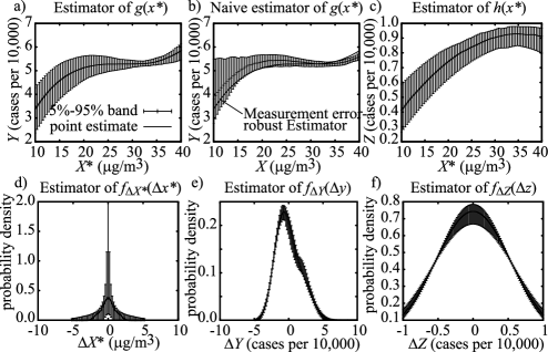
Figure 2: Application of the proposed estimator to an epidemiologic example (see text for a description of the variables and the estimated functions). In each plot, the estimator is shown as a solid line while the error bars indicate the pointwise 90% confidence bands. In (b), the “naive” estimator is a nonparametric polynomial series least-square estimator that ignores the presence of measurement error. The estimator in (a) is shown on the plot (b) for comparison.

Results are shown in Figure 2. A few observations are in order. First, our measurement error-robust estimator is perfectly able to detect a clear monotone relationship between $Y$ and $X^{\ast}$ and between $Z$ and $X^{\ast}$ with useful confidence bands, despite the use of a fully nonparametric approach. Second, although the distribution of the measurement error is difficult to estimate (as reflected by the wide confidence bands), the impact of this uncertainty on the main function of interest [$g(x^{\ast})$] is fortunately very limited. The 90% confidence bands indicate that the presence of substantial measurement error is consistent with the data: the measurement error is of the order of 10 $\mu$g/m³, whereas the observed $X$ roughly ranges from 10 to 40 $\mu$g/m³. Third, the distribution of $\Delta Y$ exhibits nonnegligible asymmetry, thus illustrating the drawbacks of methods merely assuming normality of all the error terms. In contrast, the distributions of $\Delta X^{\ast}$ and $\Delta Z$ are apparently very close to symmetric (this is a conclusion of the formal model selection procedure, not an assumption).

For comparison purposes, we also naively regress the dependent variables ($Y$ or $Z$) on the mismeasured regressor $X$ using a conventional least squares (thereby neglecting measurement error) with a polynomial specification with the same number of terms as our Berkson model. A first troubling observation from this exercise [see Figure 2(b)] is that the naive estimate of $g(x^{\ast})$ is not monotone, although in the region where it is unexpectedly decreasing, the confidence bands do not rule out a constant response. Second, it is perhaps counter-intuitive that the confidence bands for the naive estimator are sometimes larger than the corresponding bands for the measurement error-robust estimator. This is a consequence of the fact that correcting for Berkson errors amounts to an operation akin to convolution (rather than deconvolution, as in classical measurement errors). Unlike deconvolution, convolution is a noise-reducing operation, effectively averaging observations of $Y$ over a wide range of values of $X$ to yield an estimate the expected value of $Y$ given a specific value of $X$. This phenomenon is probably also responsible for the more reasonable (i.e., increasing) behavior of the response for the measurement error-robust estimate. Finally, the measurement error-robust regression function often lies at or beyond the 95% or 5% percentiles of the naive estimator distribution; see Figure 2(b). This implies that the level of any statistical test would be severely biased. For instance, the confidence bands of the naive estimator would reject our best estimate of $g(x^{\ast})$ obtained with the measurement-error robust procedure.

In summary, this application example serves to illustrate that ignoring Berkson errors can be seriously misleading in nonlinear settings. Not only is the shape of the estimated response considerably affected, but statistical inferences based on a measurement error-blind method would be seriously biased. This application example also shows that our fully nonparametric and measurement error-robust method works well at sample sizes typically available in real data sets, without assuming the knowledge of the distribution of the measurement error.

Appendix: Proofs

Let $\mathcal{L}_{1}^{b}(\mathcal{D})$ with $\mathcal{D}\subset$ $\mathbb{R}^{n_{0}}$ for some $n_{0}$ denote the set of all bounded functions in $\mathcal{L}_{1}(\mathcal{D})$ endowed with the usual $\mathcal{L}_{1}$ norm. Also, whenever we state an equality between functions in $\mathcal{L}_{1}^{b}(\mathcal{D})$, we mean that their difference is zero in the $\mathcal{L}_{1}$ norm.

We provide two proofs of Theorem 1. The first one, suggested by a referee, relies on the additional assumptions that (i) $Z$ and $X^{\ast}$ have the same dimension and (ii) $h$ and its inverse are differentiable. Assumption (i) makes Assumption 3.3 unlikely to hold, but enables a somewhat direct application of Theorem 1 in Hu and Schennach (2008). The second proof relaxes those assumptions. It borrows some of the operator techniques from Hu and Schennach (2008), yet requires considerable changes in the approach—we focus here on the aspects of the proof that differ.

Proof Theorem 3.1 (simple special case) Let variables from Hu and Schennach (2008) be denoted by the corresponding uppercase letter with tildes and make the following assignments: $(\tilde{X}^{\ast},\tilde{X},\tilde{Y},\tilde{Z})=(h(X^{\ast}),Z,Y,X)$. We now verify the 5 assumptions of Theorem 1 in Hu and Schennach (2008).

To verify Assumption 1, we observe that the densities of $(\tilde{X}^{\ast},\tilde{X},\tilde{Y},\tilde{Z})$ and $(X^{\ast},Z,Y,X)$ are related through:$f_{\tilde{X}^{\ast},\tilde{X},\tilde{Y},\tilde{Z}}(\tilde{x}^{\ast},\tilde{x},\tilde{y},\tilde{z})=f_{X^{\ast},Z,Y,X}(h^{-1}(\tilde{x}^{\ast}),\break\tilde{x},\tilde{y},\tilde{z})|{\partial h^{-1}(\tilde{x}^{\ast})}/{\partial\tilde{x}^{\ast\prime}}|$ where the density $f_{X^{\ast},Z,Y,X}$ exists by Assumption 3.1, and $h^{-1}(\tilde{x}^{\ast})$ exists by Assumption 3.3. The Jacobian $\partial h^{-1}(\tilde{x}^{\ast})/\partial\tilde{x}^{\ast\prime}$ matrix is only defined if $X^{\ast}$ and $Z$ (and therefore $\tilde{X}^{\ast}$) have the same dimension and is finite and nonsingular under the assumption that $h$ and its inverse are differentiable. A similar argument can be used for marginals and conditional distributions.

To verify Assumption 2, we note that our model can be written in terms of tilded variables as

$$\tilde{Y} = Y=g\bigl{(}h^{-1}\bigl{(}\tilde{X}^{\ast}\bigr{)}\bigr{)}+\Delta Y,$$ (17)

$$\tilde{Z} = X=h^{-1}\bigl{(}\tilde{X}^{\ast}\bigr{)}-\Delta X^{\ast},$$ (18)

$$\tilde{X} = Z=\tilde{X}^{\ast}+\Delta Z.$$ (19)

To verify Assumption 2(i), we write

$$f_{\tilde{Y}|\tilde{X},\tilde{X}^{\ast},\tilde{Z}}\bigl{(}\tilde{y}|\tilde{x},\tilde{x}^{\ast},\tilde{z}\bigr{)} = f_{Y|Z,X^{\ast},X}\bigl{(}\tilde{y}|\tilde{x},h^{-1}\bigl{(}\tilde{x}^{\ast}\bigr{)},\tilde{z}\bigr{)}$$

$$= f_{\Delta Y|\Delta Z,\Delta X^{\ast},X}\bigl{(}\tilde{y}-g\bigl{(}h^{-1}\bigl{(}\tilde{x}^{\ast}\bigr{)}\bigr{)}|\tilde{x}-\tilde{x}^{\ast},h^{-1}\bigl{(}\tilde{x}^{\ast}\bigr{)}-\tilde{z},\tilde{z}\bigr{)}$$

$$= f_{\Delta Y}\bigl{(}\tilde{y}-g\bigl{(}h^{-1}\bigl{(}\tilde{x}^{\ast}\bigr{)}\bigr{)}\bigr{)}$$

$$= f_{Y|\tilde{X}^{\ast}}\bigl{(}\tilde{y}|\tilde{x}^{\ast}\bigr{)}=f_{\tilde{Y}|\tilde{X}^{\ast}}\bigl{(}\tilde{y}|\tilde{x}^{\ast}\bigr{)},$$

where we have used, in turn, (i) the equality $(\tilde{X}^{\ast},\tilde{X},\tilde{Y},\tilde{Z})=(h(X^{\ast}),Z,Y,X)$ and the fact that changes of variables in the conditioning variables do not introduce Jacobian terms, (ii) the fact that conditioning on $Z,X^{\ast},X$ is equivalent to conditioning on $\Delta Z,\Delta X^{\ast},X$, (iii) Assumption 2.1, (iv) the relationship between $\Delta Y$ and $Y$ via (17) and (v) the equality $Y=\tilde{Y}$.

To verify Assumption 2(ii), we similarly write

$$f_{\tilde{X}|\tilde{X}^{\ast},\tilde{Z}}\bigl{(}\tilde{x}|\tilde{x}^{\ast},\tilde{z}\bigr{)} = f_{Z|X^{\ast},X}\bigl{(}\tilde{x}|h^{-1}\bigl{(}\tilde{x}^{\ast}\bigr{)},\tilde{z}\bigr{)}$$

$$= f_{\Delta Z|\Delta X^{\ast},X}\bigl{(}\tilde{x}-\tilde{x}^{\ast}|h^{-1}\bigl{(}\tilde{x}^{\ast}\bigr{)}-\tilde{z},\tilde{z}\bigr{)}$$

$$= f_{\Delta Z}\bigl{(}\tilde{x}-\tilde{x}^{\ast}\bigr{)}=f_{Z|\tilde{X}^{\ast}}\bigl{(}\tilde{x}|\tilde{x}^{\ast}\bigr{)}=f_{\tilde{X}|\tilde{X}^{\ast}}\bigl{(}\tilde{x}|\tilde{x}^{\ast}\bigr{)}.$$

Assumption 3 is implied by Assumptions 3.1, 2.1, 3.2, 3.3, 3.4 and Lemma .1 below.

Assumption 4 requires that $f_{\tilde{Y}|\tilde{X}^{\ast}}(\tilde{y}|\tilde{x}_{1}^{\ast})\not=f_{\tilde{Y}|\tilde{X}^{\ast}}(\tilde{y}|\tilde{x}_{2}^{\ast})$ for $\tilde{x}_{1}^{\ast}\not=\tilde{x}_{2}^{\ast}$. This can be verified as follows:

$$f_{\tilde{Y}|\tilde{X}^{\ast}}\bigl{(}\tilde{y}|\tilde{x}_{1}^{\ast}\bigr{)} = f_{\Delta Y|\tilde{X}^{\ast}}\bigl{(}\tilde{y}-g\bigl{(}h^{-1}\bigl{(}\tilde{x}_{1}^{\ast}\bigr{)}\bigr{)}|\tilde{x}_{1}^{\ast}\bigr{)}$$

$$= f_{\Delta Y}\bigl{(}\tilde{y}-g\bigl{(}h^{-1}\bigl{(}\tilde{x}_{1}^{\ast}\bigr{)}\bigr{)}\bigr{)}$$

$$\neq f_{\Delta Y}\bigl{(}\tilde{y}-g\bigl{(}h^{-1}\bigl{(}\tilde{x}_{2}^{\ast}\bigr{)}\bigr{)}\bigr{)}=f_{\tilde{Y}|\tilde{X}^{\ast}}\bigl{(}\tilde{y}|\tilde{x}_{2}^{\ast}\bigr{)}$$

by invoking (i) the definition of $\Delta Y$, (ii) independence of $\Delta Y$ from $X^{\ast}$ (and therefore $\tilde{X}^{\ast}$), (iii) the fact that $\tilde{x}_{1}^{\ast}\neq\tilde{x}_{2}^{\ast}$ implies $g(h^{-1}(\tilde{x}_{1}^{\ast}))\not=g(h^{-1}(\tilde{x}_{2}^{\ast}))$ since $g(\cdot)$ and $h(\cdot)$ are one-to-one by Assumption 3.3 and so is $g(h^{-1}(\cdot))$.

Assumption 5 is trivially satisfied, by equation (19).

Theorem 1 in Hu and Schennach (2008) then allows us to conclude that the joint distribution of $(h(X^{\ast}),X,Y,Z)$ is identified. However, in order to identify the distribution of $(X^{\ast},X,Y,Z)$, we need to identify $h(\cdot)$. To this effect, we note that, conditional on $X=x$, the fluctuations in $\tilde{X}^{\ast}$ are entirely caused by fluctuations in $\Delta X^{\ast}$ by equation (18). Moreover, $\Delta X^{\ast}$ is independent from $X$, hence

$$f_{\tilde{X}^{\ast}|X}\bigl{(}\tilde{x}^{\ast}|x\bigr{)}=f_{\Delta X^{\ast}}\bigl{(}h^{-1}\bigl{(}\tilde{x}^{\ast}\bigr{)}-x\bigr{)}\biggl{|}\frac{\partial h^{-1}(\tilde{x}^{\ast})}{\partial\tilde{x}^{\ast\prime}}\biggr{|},$$ (20)

where the left-hand side was previously identified and where the Jacobian term is well defined by Assumptions 3.3 and the assumed differentiability of $h^{-1}(\tilde{x}^{\ast})$. The Jacobian can be identified by integrating (20) with respect to $x^{\ast}$ to yield $\int f_{\tilde{X}^{\ast}|X}(\tilde{x}^{\ast}|x)\,dx=|\frac{\partial h^{-1}(\tilde{x}^{\ast})}{\partial\tilde{x}^{\ast\prime}}|$. By varying $x$ while keeping $\tilde{x}^{\ast}$ fixed in equation (20), we can identify the density $f_{\Delta X^{\ast}}$ up to a shift of $h^{-1}(\tilde{x}^{\ast})$. Assumption 2.2, pins down what the shift should be, so that $h^{-1}(\tilde{x}^{\ast})$ is identified for any given $\tilde{x}^{\ast}$. Since $h(\cdot)$ is one-to-one by Assumption 3.3, $h^{-1}(\cdot)$ uniquely determines $h(\cdot)$. Hence, the joint distribution of $(X^{\ast},X,Y,Z)$ is identified. Finally, noting that $f_{Y|X^{\ast}}(y|x^{\ast})=f_{\Delta Y}(y-g(x^{\ast}))$ (by Assumption 2.1), then establishes the identification of $g(x^{\ast})$ with the help of Assumption 2.2.

Proof of Theorem 3.1 (general case) This proof borrows some of the operator techniques from Hu and Schennach (2008), and we focus here on the aspects of the proof that differ.

The definition of marginal and conditional densities in combination with Assumption 2.1 lead to the following sequence of equalities:

$$f_{Y,Z|X}(y,z|x)$$

$$\qquad=\int f_{Y|X^{\ast},Z,X}\bigl{(}y|x^{\ast},z,x\bigr{)}f_{X^{\ast},Z|X}\bigl{(}x^{\ast},z|x\bigr{)}\,dx^{\ast}$$

$$\qquad=\int f_{\Delta Y|X^{\ast},\Delta Z,\Delta X^{\ast}}\bigl{(}y-g\bigl{(}x^{\ast}\bigr{)}|x^{\ast},z-h\bigl{(}x^{\ast}\bigr{)},x^{\ast}-x\bigr{)}f_{X^{\ast},Z|X}\bigl{(}x^{\ast},z|x\bigr{)}\,dx^{\ast}$$

$$\qquad=\int f_{\Delta Y}\bigl{(}y-g\bigl{(}x^{\ast}\bigr{)}\bigr{)}f_{X^{\ast},Z|X}\bigl{(}x^{\ast},z|x\bigr{)}\,dx^{\ast}$$

$$\qquad=\int f_{\Delta Y}\bigl{(}y-g\bigl{(}x^{\ast}\bigr{)}\bigr{)}f_{Z|X^{\ast},X}\bigl{(}z|x^{\ast},x\bigr{)}f_{X^{\ast}|X}\bigl{(}x^{\ast}|x\bigr{)}\,dx^{\ast}$$

$$\qquad=\int f_{\Delta Y}\bigl{(}y-g\bigl{(}x^{\ast}\bigr{)}\bigr{)}f_{\Delta Z|X^{\ast},\Delta X^{\ast}}\bigl{(}z-h\bigl{(}x^{\ast}\bigr{)}|x^{\ast},x^{\ast}-x\bigr{)}$$

$$\qquad\quad\hskip 8.5pt{}\times f_{\Delta X^{\ast}|X}\bigl{(}x^{\ast}-x|x\bigr{)}\,dx^{\ast}$$

$$\qquad=\int f_{\Delta Y}\bigl{(}y-g\bigl{(}x^{\ast}\bigr{)}\bigr{)}f_{\Delta Z}\bigl{(}z-h\bigl{(}x^{\ast}\bigr{)}\bigr{)}f_{\Delta X^{\ast}}\bigl{(}x^{\ast}-x\bigr{)}\,dx^{\ast}$$

or, equivalently,

$$f_{Y,Z|X}(y,z|x)=\int f_{Z|X^{\ast}}\bigl{(}z|x^{\ast}\bigr{)}f_{Y|X^{\ast}}\bigl{(}y|x^{\ast}\bigr{)}f_{X^{\ast}|X}\bigl{(}x^{\ast}|x\bigr{)}\,dx^{\ast}.$$ (21)

As in Hu and Schennach (2008), this integral equation can be written more conveniently as an operator equivalence relation

$$F_{y;Z|X}=F_{Z|X^{\ast}}D_{y;X^{\ast}}F_{X^{\ast}|X}$$ (22)

by introducing the operators defined in equation (3), which are acting on an arbitrary $r\in\mathcal{L}_{1}^{b}(\mathcal{X})$ [or $r\in\mathcal{L}_{1}^{b}(\mathcal{X}^{\ast})$].

Similarly, one can show that

$$f_{Z|X}(z|x)=\int f_{Z|X^{\ast}}\bigl{(}z|x^{\ast}\bigr{)}f_{X^{\ast}|X}\bigl{(}x^{\ast}|x\bigr{)}\,dx^{\ast}$$ (23)

and thus $F_{Z|X}=F_{Z|X^{\ast}}F_{X^{\ast}|X}$. By Assumptions 3.1, 2.1, 3.2, 3.3, 3.4 and Lemma .1 below, we know that $F_{Z|X^{\ast}}$ admits an inverse on the range of $F_{Z|X^{\ast}}$ (and therefore the range of $F_{Z|X}$), and we can write

$$F_{X^{\ast}|X}=F_{Z|X^{\ast}}^{-1}F_{Z|X}.$$ (24)

Substituting (24) into (22), we obtain

$$F_{y;Z|X}=F_{Z|X^{\ast}}D_{y;X^{\ast}}F_{Z|X^{\ast}}^{-1}F_{Z|X}.$$

By Assumptions 3.1, 2.1, 3.2, 3.3, 3.4 and Lemma .1 below again, $F_{Z|X}$ admits an inverse. Moreover, by Lemma 1 in Hu and Schennach (2008), the domain of $F_{Z|X}^{-1}$ is dense in $\mathcal{L}_{1}^{b}(\mathcal{Z})$, and we can then write

$$F_{y;Z|X}F_{Z|X}^{-1}=F_{Z|X^{\ast}}D_{y;X^{\ast}}F_{Z|X^{\ast}}^{-1}.$$ (25)

Equation (25) states that the operator $F_{y;Z|X}F_{Z|X}^{-1}$ admits a spectral decomposition, where the eigenvalues are given by the $f_{Y|X^{\ast}}(y|x^{\ast})$ for $x^{\ast}\in\mathcal{X}^{\ast}$ (for a fixed $y$) defining the operator $D_{y;X^{\ast}}$ while the eigenfunctions are the functions $f_{Z|X^{\ast}}(\cdot|x^{\ast})$ for $x^{\ast}\in\mathcal{X}^{\ast}$ defining the kernel of the operator $F_{Z|X^{\ast}}$. As usual, the knowledge of a linear operator [e.g., $F_{Z|X}$] only determines the value of its kernel [e.g., $f_{Z|X}(z|x)$] everywhere except on a set of null Lebesgue measure. The resulting equivalence class exactly matches the usual equivalence class for probability densities with respect to the Lebesgue measure, so identifiability of the model is not affected.

The operator to be diagonalized is entirely defined in terms of observable densities while the decomposition provides the unobserved densities of interest. To ensure uniqueness of this decomposition, we employ four techniques. First, a powerful result from spectral analysis [Theorem XV 4.5 in Dunford and Schwartz (1971)] ensures uniqueness up to some normalizations. Second, the a priori arbitrary scale of the eigenfunctions is fixed by the requirement that densities must integrate to one. Third, to avoid any ambiguity in the definition of the eigenfunctions when degenerate eigenvalues are present, we use Assumption 3.3 and the fact that the eigenfunctions [which do not depend on $y$, unlike the eigenvalues $f_{y|x^{\ast}}(y|x^{\ast})$] must be consistent across different values of the dependent variable $y$. These three steps are described in detail in Hu and Schennach (2008) and are not repeated here.

The fourth step [which differs from the approach taken in Hu and Schennach (2008)] is to rule out that the eigenvalues $f_{y;X^{\ast}}(y,x^{\ast})$ and eigenfunctions $f_{Z|X^{\ast}}(\cdot|x^{\ast})$ could be indexed by a different variable without affecting the operator $F_{y;Z|X}F_{Z|X}^{-1}$. (This issue is analogous to the nonunique ordering of the eigenvalues and eigenvectors in matrix diagonalization.) Suppose that the eigenfunctions can be indexed by another value, that is, they are given by $f_{Z|\tilde{X}^{\ast}}(\cdot|\tilde{x}^{\ast})$ where $\tilde{x}^{\ast}$ is another variable related to $x^{\ast}$ through $x^{\ast}=S(\tilde{x}^{\ast})$ for some one-to-one function $S$. Under this alternative indexing, all the assumptions of the original model must still hold with $x^{\ast}$ replaced by $\tilde{x}^{\ast}$, so a relationship similar to (23) would still have to hold, for the same observed $f_{Z|X}(z|x)$

$$f_{Z|X}(z|x)=\int f_{Z|\tilde{X}^{\ast}}\bigl{(}z|\tilde{x}^{\ast}\bigr{)}f_{\tilde{X}^{\ast}|X}\bigl{(}\tilde{x}^{\ast}|x\bigr{)}\,d\tilde{x}^{\ast}$$ (26)

or, in operator notation, $F_{Z|X}=F_{Z|\tilde{X}^{\ast}}F_{\tilde{X}^{\ast}|X}$.

In order for $f_{Z|\tilde{X}^{\ast}}(z|\tilde{x}^{\ast})$ to be a valid alternative density, it must satisfy the same assumptions (and their implications) as $f_{Z|X^{\ast}}(z|x^{\ast})$. In particular, the fact that $F_{Z|X^{\ast}}$ is invertible (established above via Lemma .1) must also hold for $F_{Z|\tilde{X}^{\ast}}$. Hence, for any alternative $F_{Z|\tilde{X}^{\ast}}$, there is a unique corresponding $F_{\tilde{X}^{\ast}|X}$, given by $F_{\tilde{X}^{\ast}|X}=F_{Z|\tilde{X}^{\ast}}^{-1}F_{Z|X}$. We can find a more explicit expression for $f_{\tilde{X}^{\ast}|X}(\tilde{x}^{\ast}|x)$ as follows. First note that we trivially have that $f_{Z|\tilde{X}^{\ast}}(z|\tilde{x}^{\ast})=f_{Z|X^{\ast}}(z|S(\tilde{x}^{\ast}))$ since $x^{\ast}=S(\tilde{x}^{\ast})$ and $S$ is one-to-one. By performing the change of variable $x^{\ast}=S(\tilde{x}^{\ast})$ in (23), we obtain

$$f_{Z|X}(z|x)=\int f_{Z|X^{\ast}}\bigl{(}z|S\bigl{(}\tilde{x}^{\ast}\bigr{)}\bigr{)}f_{X^{\ast}|X}\bigl{(}S\bigl{(}\tilde{x}^{\ast}\bigr{)}|x\bigr{)}\,d\mu\bigl{(}\tilde{x}^{\ast}\bigr{)},$$

where the measure $\mu$ is defined, via $\mu(\mathcal{A})=\lambda(S^{-1}(\mathcal{A}))$ for any measurable set $\mathcal{A}$, where $\lambda$ denotes the Lebesgue measure and $S^{-1}(\mathcal{A})\equiv\{\tilde{x}^{\ast}\in\mathcal{A}:S(\tilde{x}^{\ast})=x^{\ast}\}$. From this we can conclude the equality between the two following measures:

$$f_{\tilde{X}^{\ast}|X}\bigl{(}\tilde{x}^{\ast}|x\bigr{)}\,d\tilde{x}^{\ast}=f_{X^{\ast}|X}\bigl{(}S\bigl{(}\tilde{x}^{\ast}\bigr{)}|x\bigr{)}\,d\mu\bigl{(}\tilde{x}^{\ast}\bigr{)}$$ (27)

by comparison to equation (26) and the uniqueness of the measure$f_{\tilde{X}^{\ast}|X}(\tilde{x}^{\ast}|x)\,d\tilde{x}^{\ast}$ due to the injectivity of the $F_{Z|\tilde{X}^{\ast}}$ operator, shown in Lemma .1 in the general case where the domain of $F_{Z|\tilde{X}^{\ast}}$ could include finite signed measures. We will now show that $f_{\tilde{X}^{\ast}|X}(\tilde{x}^{\ast}|x)$ necessarily violates Assumption 2.2 (with $\Delta X^{\ast}$ replaced by $\Delta\tilde{X}^{\ast}\equiv\tilde{X}^{\ast}-X$), unless $S(\cdot)$ is the identity function.

Since $\Delta X^{\ast}=X^{\ast}-X$ with $\Delta X^{\ast}$ independent from $X$, we have $f_{X^{\ast}|X}(x^{\ast}|x)=f_{\Delta X^{\ast}}(x^{\ast}-x)$ and by a similar reasoning $f_{\tilde{X}^{\ast}|X}(\tilde{x}^{\ast}|x)=f_{\Delta\tilde{X}^{\ast}}(\tilde{x}^{\ast}-x)$ with $\Delta\tilde{X}^{\ast}\equiv\tilde{X}^{\ast}-X$. Equation (27) then becomes

$$f_{\Delta\tilde{X}^{\ast}}\bigl{(}\tilde{x}^{\ast}-x\bigr{)}\,d\tilde{x}^{\ast}=f_{\Delta X^{\ast}}\bigl{(}S\bigl{(}\tilde{x}^{\ast}\bigr{)}-x\bigr{)}\,d\mu\bigl{(}\tilde{x}^{\ast}\bigr{)}.$$ (28)

Now, for a given $x$, consider Radom–Nikodym derivative of $f_{\Delta\tilde{X}^{\ast}}(\tilde{x}^{\ast}-x)\,d\tilde{x}^{\ast}$ with respect to the Lebesgue measure $d\tilde{x}^{\ast}$, which is, by definition (almost everywhere) equal to $f_{\Delta\tilde{X}^{\ast}}(\tilde{x}^{\ast}-x)$, a bounded function by Assumption 3.1. By equation (28), the existence of the Radom–Nikodym derivative of the left-hand side implies the existence of the same Radom–Nikodym derivative on the right-hand side, and we can write

$$f_{\Delta\tilde{X}^{\ast}}\bigl{(}\tilde{x}^{\ast}-x\bigr{)}=f_{\Delta X^{\ast}}\bigl{(}S\bigl{(}\tilde{x}^{\ast}\bigr{)}-x\bigr{)}\,\frac{d\mu(\tilde{x}^{\ast})}{d\tilde{x}^{\ast}}$$ (29)

almost everywhere. Integrating both sides of the equation over all $x\in\mathcal{X}$, we obtain (after noting that points where the equality may fail have null measure and therefore do not contribute to the integral), $1=1\,\frac{d\mu(\tilde{x}^{\ast})}{d\tilde{x}^{\ast}}$, since densities integrate to $1$, which implies that $d\mu(\tilde{x}^{\ast})/d\tilde{x}^{\ast}=1$, that is, $\mu$ is also the Lebesgue measure. It follows from (29) that, almost everywhere

$$f_{\Delta\tilde{X}^{\ast}}\bigl{(}\tilde{x}^{\ast}-x\bigr{)}=f_{\Delta X^{\ast}}\bigl{(}S\bigl{(}\tilde{x}^{\ast}\bigr{)}-x\bigr{)}.$$

In order for Assumption 2.2 to hold for both $\Delta\tilde{X}^{\ast}$ and $\Delta X^{\ast}$, we must have that $f_{\Delta\tilde{X}^{\ast}}(\tilde{x}^{\ast}-x)$, when viewed as a function of $\tilde{x}^{\ast}$ for any given $x$, is centered at $\tilde{x}^{\ast}=x$, and we must simultaneously have that $f_{\Delta X^{\ast}}(x^{\ast}-x)=f_{\Delta X^{\ast}}(S(\tilde{x}^{\ast})-x)$, when viewed as a function of $x^{\ast}$ for any given $x$, is centered at $x^{\ast}=x$, that is, $S(\tilde{x}^{\ast})=x$. The two statements are only compatible if $\tilde{x}^{\ast}=S(\tilde{x}^{\ast})$. Thus, there cannot exist two distinct but observationally equivalent parametrization of the eigenvalues/eigenfunctions.

Hence we have shown, through equation (25), that the unobserved functions $f_{Y|X^{\ast}}(y|x^{\ast})$ and $f_{Z|X^{\ast}}(\cdot|x^{\ast})$ are uniquely determined (up to an equivalence class of functions differing at most on a set of null Lebesgue measure) by the observed function $f_{Y,Z|X}(y,z|x)$. Next, equation (24) implies that $f_{X^{\ast}|X}(x^{\ast}|x)$ is uniquely determined as well.

Once $f_{Y|X^{\ast}}(y|x^{\ast})$ and $f_{Z|X^{\ast}}(z|x^{\ast})$ are known, the functions $g(x^{\ast})$ and $h(x^{\ast})$ can be identified by exploiting the centering restrictions on $\Delta Y$, $\Delta X^{\ast}$ and $\Delta Z$, for example, $g(x^{\ast})=\int yf_{Y|X^{\ast}}(y|x^{\ast})\,dy$ if $\Delta Y$ is assumed to have zero mean. Next, $f_{\Delta Y}(\Delta y)$ can be straightforwardly identified, for example, $f_{\Delta Y}(\Delta y)=f_{Y|X^{\ast}}(g(x^{\ast})+\Delta y|x^{\ast})$ for any $x^{\ast}\in\mathcal{X}^{\ast}$. Similar arguments yield $h(x^{\ast})$ and $f_{\Delta Z}(\Delta z)$ from $f_{Z|X^{\ast}}(z|x^{\ast})$ as well as $f_{\Delta X^{\ast}}(\Delta x^{\ast})$ from $f_{X^{\ast}|X}(x^{\ast}|x)$. It follows that equation (4) has a unique solution. The second conclusion of the theorem then follows from the fact that both $f_{Y,Z|X}(y,z|x)$ and $f_{X}(x)$ are uniquely determined (except perhaps on a set of null Lebesgue measure) from $f_{Y,Z,X}(y,z,x)$.

The following lemma is closely related to Proposition 2.4 in D’Haultfoeuille (2011). It is different in terms of the spaces the operators can act on and more general in terms of the possible dimensionalities of the random variables involved.

Lemma .1

Let $X,X^{\ast}$ and $Z$ be generated by equations (2) and (3). Let $\mathcal{S}(\mathcal{T})$ be the set of finite signed measures on a given set $\mathcal{T=X},\mathcal{X}^{\ast}$ or $\mathcal{Z}$ [and note that $\mathcal{S}(\mathcal{T})$ includes $\mathcal{L}_{1}^{b}(\mathcal{T})$ as a special case, in the sense that for any function in $r\in\mathcal{L}_{1}^{b}(\mathcal{T})$, there is a corresponding measure $R\in\mathcal{S}(\mathcal{T})$ whose Radom–Nikodym derivative with respect to the Lebesgue measure is $r$]. Under Assumptions 2.1, 3.1, 3.2, 3.3 and 3.4, the operators $F_{X^{\ast}|X}\dvtx\mathcal{S}(\mathcal{X})\mapsto\mathcal{L}_{1}^{b}(\mathcal{X}^{\ast})$, $F_{Z|X^{\ast}}\dvtx\mathcal{S}(\mathcal{X}^{\ast})\mapsto\mathcal{L}_{1}^{b}(\mathcal{Z})$ and $F_{Z|X}\dvtx\mathcal{S}(\mathcal{X})\mapsto\mathcal{L}_{1}^{b}(\mathcal{Z})$, defined in (3), are injective mappings.

First, one can verify that $R\in\mathcal{S}(\mathcal{X})$ implies that $F_{X^{\ast}|X}R\in\mathcal{L}_{1}^{b}(\mathcal{X}^{\ast})$ and similarly for $F_{Z|X^{\ast}}$ and $F_{Z|X}$, since the (conditional) densities involving variables $X^{\ast},X$ and $Z$ are bounded by Assumption 3.1 and are absolutely integrable. We now verify injectivity of $F_{Z|X^{\ast}}$.

By Assumptions 2.1, 3.1 and equation (3), we have, for any $R\in\mathcal{S}(\mathcal{X}^{\ast})$,

$$[F_{Z|X^{\ast}}R](z)=\int f_{Z|X^{\ast}}\bigl{(}z|x^{\ast}\bigr{)}\,dR\bigl{(}x^{\ast}\bigr{)}=\int f_{\Delta Z}\bigl{(}z-h\bigl{(}x^{\ast}\bigr{)}\bigr{)}\,dR\bigl{(}x^{\ast}\bigr{)}.$$

Next, let $\tilde{R}$ denote the signed measure assigning, to any measurable set $\mathcal{A}\subseteq\mathbb{R}^{n_{z}}$, the value$\tilde{R}(\mathcal{A})=\int 1(h(x^{\ast})\in\mathcal{A})\,dR(x^{\ast})$ and note that $\tilde{R}$ is a finite signed measure since $R(x^{\ast})$ is. Then, we can express $F_{Z|X^{\ast}}R$ as

$$[F_{Z|X^{\ast}}R](z)=\int f_{\Delta Z}\bigl{(}z-\tilde{x}^{\ast}\bigr{)}\,d\tilde{R}\bigl{(}\tilde{x}^{\ast}\bigr{)},$$ (30)

that is, a convolution between the probability measure of $\Delta Z$ (represented by its Lebesgue density) and the signed measure $\tilde{R}$; see Chapter 5 in Bhattacharya and Rao (2010). By the convolution theorem for signed measures [Theorem 5.1(iii) in Bhattacharya and Rao (2010)], one can convert the convolution (30) into a product of Fourier transforms,

$$\sigma(\zeta)=\phi_{\Delta Z}(\zeta)\rho(\zeta)$$

where $\sigma(\zeta)\equiv\int[F_{Z|X^{\ast}}R](z)e^{\mathbf{i}\zeta z}\,dz$, $\phi_{\Delta Z}(\zeta)\equiv E[e^{\mathbf{i}\zeta Z}]$ and $\rho(\zeta)\equiv\int e^{\mathbf{i}\zeta z}\,d\tilde{R}(z)$. Since $\phi_{\Delta Z}(\zeta)$, the characteristic function of $\Delta Z$, is nonvanishing by Assumption 3.2, we can isolate $\rho(\zeta)$ as

$$\rho(\zeta)=\sigma(\zeta)/\phi_{\Delta Z}(\zeta).$$

Since there is a one-to-one mapping between finite signed measures and their Fourier transforms [by Theorem 5.1(i) in Bhattacharya and Rao (2010)], $\tilde{R}$ can be recovered as the unique signed measure whose Fourier transform is $\rho(\zeta)$. We now show that the signed measure $\tilde{R}$ uniquely determines the measure $R$.

Let $\mathcal{A}_{\mathcal{B}}=\bigcup_{x^{\ast}\in\mathcal{B}}\{h(x^{\ast})\}$ for any measurable $\mathcal{B}\subseteq\mathbb{R}^{n_{x}}$, and note that $\mathcal{A}_{\mathcal{B}}$ is also measurable since $h$ is continuous by Assumption 3.4. Then observe that by Assumption 3.3, $h(x^{\ast})\in\mathcal{A}_{\mathcal{B}}$ if and only if $x^{\ast}\in\mathcal{B}$, and we have

$$\tilde{R}(\mathcal{A}_{\mathcal{B}})=\int 1\bigl{(}h\bigl{(}x^{\ast}\bigr{)}\in\mathcal{A}_{\mathcal{B}}\bigr{)}\,dR\bigl{(}x^{\ast}\bigr{)}=\int 1\bigl{(}x^{\ast}\in\mathcal{B}\bigr{)}\,dR\bigl{(}x^{\ast}\bigr{)}.$$

Since $\mathcal{B}$ is arbitrary, the knowledge of $\tilde{R}(\mathcal{A}_{\mathcal{B}})$ uniquely determines the value assigned to any measurable set by the signed measure $R$.

Injectivity of $F_{X^{\ast}|X}$ is a special case of the above derivation (with $Z,X^{\ast}$ replaced by $X^{\ast},X$), in which $h$ is the identity function. Finally, injectivity of $F_{Z|X}$ is implied by the injectivity of $F_{Z|X^{\ast}}$ and $F_{X^{\ast}|X}$, since $F_{Z|X}=F_{Z|X^{\ast}}F_{X^{\ast}|X}$ by Assumption 2.1 and equations (2) and (3).

Supplementary material to “Regressions with Berkson errors in covariates—A nonparametric approach” [doi]10.1214/13-AOS1122SUPP .pdf aos1122_supp.pdf The supplementary material provides (i) a proof of consistency of the proposed estimator, (ii) additional simulation results and (iii) various extensions of the method, including the weakening of some of full independence assumptions to conditional independence and handling the simultaneous presence of classical and Berkson errors.

References

- Berkson (1950) {barticle}[author] \bauthor\bsnmBerkson, \bfnmJ.\binitsJ. (\byear1950). \btitleAre there two regressions? \bjournalJ. Amer. Statist. Assoc. \bvolume45 \bpages164–180. \bptokimsref \endbibitem
- Bhattacharya and Rao (2010) {bbook}[author] \bauthor\bsnmBhattacharya, \bfnmR. N.\binitsR. N. and \bauthor\bsnmRao, \bfnmR. R.\binitsR. R. (\byear2010). \btitleNormal Approximation and Asymptotic Expansions. \bpublisherSIAM, \blocationPhiladelphia. \bptokimsref \endbibitem
- Carrasco, Florens and Renault (2005) {bincollection}[author] \bauthor\bsnmCarrasco, \bfnmM.\binitsM., \bauthor\bsnmFlorens, \bfnmJ. P.\binitsJ. P. and \bauthor\bsnmRenault, \bfnmE.\binitsE. (\byear2005). \btitleLinear inverse problems and structural econometrics: Estimation based on spectral decomposition and regularization. In \bbooktitleHandbook of Econometrics, Vol. 6. \bpublisherElsevier, \blocationAmsterdam. \bptokimsref \endbibitem
- Carroll, Chen and Hu (2010) {barticle}[mr] \bauthor\bsnmCarroll, \bfnmRaymond J.\binitsR. J., \bauthor\bsnmChen, \bfnmXiaohong\binitsX. and \bauthor\bsnmHu, \bfnmYingyao\binitsY. (\byear2010). \btitleIdentification and estimation of nonlinear models using two samples with nonclassical measurement errors. \bjournalJ. Nonparametr. Stat. \bvolume22 \bpages379–399. \biddoi=10.1080/10485250902874688, issn=1048-5252, mr=2662599 \bptokimsref \endbibitem
- Carroll, Delaigle and Hall (2007) {barticle}[mr] \bauthor\bsnmCarroll, \bfnmRaymond J.\binitsR. J., \bauthor\bsnmDelaigle, \bfnmAurore\binitsA. and \bauthor\bsnmHall, \bfnmPeter\binitsP. (\byear2007). \btitleNon-parametric regression estimation from data contaminated by a mixture of Berkson and classical errors. \bjournalJ. R. Stat. Soc. Ser. B Stat. Methodol. \bvolume69 \bpages859–878. \biddoi=10.1111/j.1467-9868.2007.00614.x, issn=1369-7412, mr=2368574 \bptokimsref \endbibitem
- Carroll et al. (2006) {bbook}[mr] \bauthor\bsnmCarroll, \bfnmRaymond J.\binitsR. J., \bauthor\bsnmRuppert, \bfnmDavid\binitsD., \bauthor\bsnmStefanski, \bfnmLeonard A.\binitsL. A. and \bauthor\bsnmCrainiceanu, \bfnmCiprian M.\binitsC. M. (\byear2006). \btitleMeasurement Error in Nonlinear Models. \bpublisherChapman & Hall/CRC, \blocationBoca Raton, FL. \bptokimsref \endbibitem
- Delaigle, Hall and Qiu (2006) {barticle}[mr] \bauthor\bsnmDelaigle, \bfnmAurore\binitsA., \bauthor\bsnmHall, \bfnmPeter\binitsP. and \bauthor\bsnmQiu, \bfnmPeihua\binitsP. (\byear2006). \btitleNonparametric methods for solving the Berkson errors-in-variables problem. \bjournalJ. R. Stat. Soc. Ser. B Stat. Methodol. \bvolume68 \bpages201–220. \biddoi=10.1111/j.1467-9868.2006.00540.x, issn=1369-7412, mr=2188982 \bptokimsref \endbibitem
- D’Haultfoeuille (2011) {barticle}[mr] \bauthor\bsnmD’Haultfoeuille, \bfnmXavier\binitsX. (\byear2011). \btitleOn the completeness condition in nonparametric instrumental problems. \bjournalEconometric Theory \bvolume27 \bpages460–471. \biddoi=10.1017/S0266466610000368, issn=0266-4666, mr=2806256 \bptokimsref \endbibitem
- Dockery et al. (1993) {barticle}[author] \bauthor\bsnmDockery, \bfnmD. W.\binitsD. W., \bauthor\bsnmPope, \bfnmC. A.\binitsC. A., \bauthor\bsnmXu, \bfnmX. P.\binitsX. P. \betalet al. (\byear1993). \btitleAn association between air-pollution and mortality in 6 United-States cities. \bjournalNew England Journal of Medicine \bvolume329 \bpages1753–1759. \bptokimsref \endbibitem
- Dunford and Schwartz (1971) {bbook}[author] \bauthor\bsnmDunford, \bfnmN.\binitsN. and \bauthor\bsnmSchwartz, \bfnmJ. T.\binitsJ. T. (\byear1971). \btitleLinear Operators. \bpublisherWiley, \blocationNew York. \bptokimsref \endbibitem
- Fan and Truong (1993) {barticle}[mr] \bauthor\bsnmFan, \bfnmJianqing\binitsJ. and \bauthor\bsnmTruong, \bfnmYoung K.\binitsY. K. (\byear1993). \btitleNonparametric regression with errors in variables. \bjournalAnn. Statist. \bvolume21 \bpages1900–1925. \biddoi=10.1214/aos/1176349402, issn=0090-5364, mr=1245773 \bptokimsref \endbibitem
- Gallant and Nychka (1987) {barticle}[mr] \bauthor\bsnmGallant, \bfnmA. Ronald\binitsA. R. and \bauthor\bsnmNychka, \bfnmDouglas W.\binitsD. W. (\byear1987). \btitleSemi-nonparametric maximum likelihood estimation. \bjournalEconometrica \bvolume55 \bpages363–390. \biddoi=10.2307/1913241, issn=0012-9682, mr=0882100 \bptokimsref \endbibitem
- Giné and Zinn (1990) {barticle}[mr] \bauthor\bsnmGiné, \bfnmEvarist\binitsE. and \bauthor\bsnmZinn, \bfnmJoel\binitsJ. (\byear1990). \btitleBootstrapping general empirical measures. \bjournalAnn. Probab. \bvolume18 \bpages851–869. \bidissn=0091-1798, mr=1055437 \bptokimsref \endbibitem
- Grenander (1981) {bbook}[mr] \bauthor\bsnmGrenander, \bfnmUlf\binitsU. (\byear1981). \btitleAbstract Inference. \bpublisherWiley, \blocationNew York. \bidmr=0599175 \bptokimsref \endbibitem
- Hausman, Newey and Powell (1995) {barticle}[mr] \bauthor\bsnmHausman, \bfnmJ. A.\binitsJ. A., \bauthor\bsnmNewey, \bfnmW. K.\binitsW. K. and \bauthor\bsnmPowell, \bfnmJ. L.\binitsJ. L. (\byear1995). \btitleNonlinear errors in variables: Estimation of some Engel curves. \bjournalJ. Econometrics \bvolume65 \bpages205–233. \biddoi=10.1016/0304-4076(94)01602-V, issn=0304-4076, mr=1324193 \bptokimsref \endbibitem
- Hausman et al. (1991) {barticle}[mr] \bauthor\bsnmHausman, \bfnmJerry A.\binitsJ. A., \bauthor\bsnmNewey, \bfnmWhitney K.\binitsW. K., \bauthor\bsnmIchimura, \bfnmHidehiko\binitsH. and \bauthor\bsnmPowell, \bfnmJames L.\binitsJ. L. (\byear1991). \btitleIdentification and estimation of polynomial errors-in-variables models. \bjournalJ. Econometrics \bvolume50 \bpages273–295. \biddoi=10.1016/0304-4076(91)90022-6, issn=0304-4076, mr=1147115 \bptokimsref \endbibitem
- Hu and Schennach (2008) {barticle}[mr] \bauthor\bsnmHu, \bfnmYingyao\binitsY. and \bauthor\bsnmSchennach, \bfnmSusanne M.\binitsS. M. (\byear2008). \btitleInstrumental variable treatment of nonclassical measurement error models. \bjournalEconometrica \bvolume76 \bpages195–216. \biddoi=10.1111/j.0012-9682.2008.00823.x, issn=0012-9682, mr=2374986 \bptokimsref \endbibitem
- Huwang and Huang (2000) {barticle}[mr] \bauthor\bsnmHuwang, \bfnmLongcheen\binitsL. and \bauthor\bsnmHuang, \bfnmY. H. Steve\binitsY. H. S. (\byear2000). \btitleOn errors-in-variables in polynomial regression-Berkson case. \bjournalStatist. Sinica \bvolume10 \bpages923–936. \bidissn=1017-0405, mr=1787786 \bptokimsref \endbibitem
- Hyslop and Imbens (2001) {barticle}[mr] \bauthor\bsnmHyslop, \bfnmDean R.\binitsD. R. and \bauthor\bsnmImbens, \bfnmGuido W.\binitsG. W. (\byear2001). \btitleBias from classical and other forms of measurement error. \bjournalJ. Bus. Econom. Statist. \bvolume19 \bpages475–481. \biddoi=10.1198/07350010152596727, issn=0735-0015, mr=1963378 \bptokimsref \endbibitem
- Lewbel (1996) {barticle}[author] \bauthor\bsnmLewbel, \bfnmA.\binitsA. (\byear1996). \btitleDemand estimation with expenditure measurement errors on the left and right hand side. \bjournalRev. Econom. Statist. \bvolume78 \bpages718–725. \bptokimsref \endbibitem
- Li (2002) {barticle}[mr] \bauthor\bsnmLi, \bfnmTong\binitsT. (\byear2002). \btitleRobust and consistent estimation of nonlinear errors-in-variables models. \bjournalJ. Econometrics \bvolume110 \bpages1–26. \biddoi=10.1016/S0304-4076(02)00120-3, issn=0304-4076, mr=1920960 \bptokimsref \endbibitem
- Li and Vuong (1998) {barticle}[mr] \bauthor\bsnmLi, \bfnmTong\binitsT. and \bauthor\bsnmVuong, \bfnmQuang\binitsQ. (\byear1998). \btitleNonparametric estimation of the measurement error model using multiple indicators. \bjournalJ. Multivariate Anal. \bvolume65 \bpages139–165. \biddoi=10.1006/jmva.1998.1741, issn=0047-259X, mr=1625869 \bptokimsref \endbibitem
- Mahajan (2006) {barticle}[mr] \bauthor\bsnmMahajan, \bfnmAprajit\binitsA. (\byear2006). \btitleIdentification and estimation of regression models with misclassification. \bjournalEconometrica \bvolume74 \bpages631–665. \biddoi=10.1111/j.1468-0262.2006.00677.x, issn=0012-9682, mr=2217611 \bptokimsref \endbibitem
- Mallick, Hoffman and Carroll (2002) {barticle}[mr] \bauthor\bsnmMallick, \bfnmBani\binitsB., \bauthor\bsnmHoffman, \bfnmF. Owen\binitsF. O. and \bauthor\bsnmCarroll, \bfnmRaymond J.\binitsR. J. (\byear2002). \btitleSemiparametric regression modeling with mixtures of Berkson and classical error, with application to fallout from the Nevada test site. \bjournalBiometrics \bvolume58 \bpages13–20. \biddoi=10.1111/j.0006-341X.2002.00013.x, issn=0006-341X, mr=1891038 \bptokimsref \endbibitem
- Nelder and Mead (1965) {barticle}[author] \bauthor\bsnmNelder, \bfnmJ. A.\binitsJ. A. and \bauthor\bsnmMead, \bfnmR.\binitsR. (\byear1965). \btitleA simplex method for function minimization. \bjournalComputer Journal \bvolume7 \bpages308–313. \bptokimsref \endbibitem
- Newey (1997) {barticle}[mr] \bauthor\bsnmNewey, \bfnmWhitney K.\binitsW. K. (\byear1997). \btitleConvergence rates and asymptotic normality for series estimators. \bjournalJ. Econometrics \bvolume79 \bpages147–168. \biddoi=10.1016/S0304-4076(97)00011-0, issn=0304-4076, mr=1457700 \bptokimsref \endbibitem
- Newey (2001) {barticle}[author] \bauthor\bsnmNewey, \bfnmW.\binitsW. (\byear2001). \btitleFlexible simulated moment estimation of nonlinear errors-in-variables models. \bjournalRev. Econom. Statist. \bvolume83 \bpages616–627. \bptokimsref \endbibitem
- Newey and Powell (2003) {barticle}[mr] \bauthor\bsnmNewey, \bfnmWhitney K.\binitsW. K. and \bauthor\bsnmPowell, \bfnmJames L.\binitsJ. L. (\byear2003). \btitleInstrumental variable estimation of nonparametric models. \bjournalEconometrica \bvolume71 \bpages1565–1578. \biddoi=10.1111/1468-0262.00459, issn=0012-9682, mr=2000257 \bptokimsref \endbibitem
- Pope et al. (1995) {barticle}[author] \bauthor\bsnmPope, \bfnmC. A.\binitsC. A., \bauthor\bsnmThun, \bfnmM. J.\binitsM. J., \bauthor\bsnmNamboodiri, \bfnmM. M.\binitsM. M. \betalet al. (\byear1995). \btitleParticulate air-pollution as a predictor of mortality in a prospective-study of us adults. \bjournalAmerican Journal of Respiratory and Critical Care Medicine \bvolume151 \bpages669–674. \bptokimsref \endbibitem
- Samet et al. (2000) {barticle}[author] \bauthor\bsnmSamet, \bfnmJ. M.\binitsJ. M., \bauthor\bsnmDominici, \bfnmF.\binitsF., \bauthor\bsnmCurriero, \bfnmF. C.\binitsF. C. \betalet al. (\byear2000). \btitleFine particulate air pollution and mortality in 20 US cities, 1987–1994. \bjournalNew England Journal of Medicine \bvolume343 \bpages1742–1749. \bptokimsref \endbibitem
- Schennach (2004) {barticle}[mr] \bauthor\bsnmSchennach, \bfnmSusanne M.\binitsS. M. (\byear2004). \btitleEstimation of nonlinear models with measurement error. \bjournalEconometrica \bvolume72 \bpages33–75. \biddoi=10.1111/j.1468-0262.2004.00477.x, issn=0012-9682, mr=2031013 \bptokimsref \endbibitem
- Schennach (2007) {barticle}[mr] \bauthor\bsnmSchennach, \bfnmSusanne M.\binitsS. M. (\byear2007). \btitleInstrumental variable estimation of nonlinear errors-in-variables models. \bjournalEconometrica \bvolume75 \bpages201–239. \biddoi=10.1111/j.1468-0262.2007.00736.x, issn=0012-9682, mr=2284741 \bptokimsref \endbibitem
- Schennach (2013) {bmisc}[author] \bauthor\bsnmSchennach, \bfnmS. M.\binitsS. M. (\byear2013). \btitleSupplement to “Regressions with Berkson errors in covariates—A nonparametric approach.” DOI:\doiurl10.1214/13-AOS1122SUPP. \bptokimsref \endbibitem
- Shen (1997) {barticle}[mr] \bauthor\bsnmShen, \bfnmXiaotong\binitsX. (\byear1997). \btitleOn methods of sieves and penalization. \bjournalAnn. Statist. \bvolume25 \bpages2555–2591. \biddoi=10.1214/aos/1030741085, issn=0090-5364, mr=1604416 \bptokimsref \endbibitem
- Stram, Huberman and Wu (2002) {barticle}[pbm] \bauthor\bsnmStram, \bfnmDaniel O.\binitsD. O., \bauthor\bsnmHuberman, \bfnmMark\binitsM. and \bauthor\bsnmWu, \bfnmAnna H.\binitsA. H. (\byear2002). \btitleIs residual confounding a reasonable explanation for the apparent protective effects of beta-carotene found in epidemiologic studies of lung cancer in smokers? \bjournalAm. J. Epidemiol. \bvolume155 \bpages622–628. \bidissn=0002-9262, pmid=11914189 \bptokimsref \endbibitem
- van der Laan, Dudoit and Keles (2004) {barticle}[mr] \bauthor\bparticlevan der \bsnmLaan, \bfnmMark J.\binitsM. J., \bauthor\bsnmDudoit, \bfnmSandrine\binitsS. and \bauthor\bsnmKeles, \bfnmSunduz\binitsS. (\byear2004). \btitleAsymptotic optimality of likelihood-based cross-validation. \bjournalStat. Appl. Genet. Mol. Biol. \bvolume3 \bpagesArt. 4, 27 pp. (electronic). \biddoi=10.2202/1544-6115.1036, issn=1544-6115, mr=2101455 \bptokimsref \endbibitem
- Wang (2004) {barticle}[mr] \bauthor\bsnmWang, \bfnmLiqun\binitsL. (\byear2004). \btitleEstimation of nonlinear models with Berkson measurement errors. \bjournalAnn. Statist. \bvolume32 \bpages2559–2579. \biddoi=10.1214/009053604000000670, issn=0090-5364, mr=2153995 \bptokimsref \endbibitem
- Wang (2007) {barticle}[mr] \bauthor\bsnmWang, \bfnmLiqun\binitsL. (\byear2007). \btitleA unified approach to estimation of nonlinear mixed effects and Berkson measurement error models. \bjournalCanad. J. Statist. \bvolume35 \bpages233–248. \biddoi=10.1002/cjs.5550350203, issn=0319-5724, mr=2393607 \bptokimsref \endbibitem