Combining data from multiple spatially referenced prevalence surveys using generalized linear geostatistical models

Abstract

Data from multiple prevalence surveys can provide information on common parameters of interest, which can therefore be estimated more precisely in a joint analysis than by separate analyses of the data from each survey. However, fitting a single model to the combined data from multiple surveys is inadvisable without testing the implicit assumption that all of the surveys are directed at the same inferential target. In this paper we propose a multivariate generalized linear geostatistical model that accommodates two sources of heterogeneity across surveys so as to correct for spatially structured bias in non-randomised surveys and to allow for temporal variation in the underlying prevalence surface between consecutive survey-periods.

We describe a Monte Carlo maximum likelihood procedure for parameter estimation, and show through simulation experiments how accounting for the different sources of heterogeneity among surveys in a joint model leads to more precise inferences. We describe an application to multiple surveys of malaria prevalence conducted in Chikhwawa District, Southern Malawi, and discuss how this approach could inform hybrid sampling strategies that combine data from randomised and non-randomised surveys so as to make the most efficient use of all available data.

Keywords: convenience sampling; generalized linear geostatistical models; malaria mapping; Monte Carlo maximum likelihood; multiple surveys; spatio-temporal models.

1. Medical School, Lancaster University, Lancaster, UK
2. Institute of Infection and Global Health, University of Liverpool, Liverpool, UK
3. Malawi-Liverpool-Wellcome Trust Clinical Research Programme, Blantyre, Malawi.
4. Liverpool School of Tropical Medicine, Liverpool, UK

1 Introduction

In studies of spatial variation in disease prevalence, it is often necessary to combine information from multiple prevalence surveys. This is particularly the case in low-resource settings, where disease registries typically do not exist. A methodological challenge in these circumstances is that survey designs are severely constrained by cost constraints. The available surveys may therefore be of variable quality and/or conducted at different times. In this paper, we propose a class of generalized linear geostatistical models (GLGMs) to address two specific issues.The first is variation in quality, for example between randomised and non-randomised surveys, in which case our proposed methodology assumes that at least one of the surveys provides an unbiased “gold-standard”. The second is variation in the underlying prevalence when surveys are conducted at different times. In this case, by modelling the underlying prevalence over time we are able to use data collected at all times to estimate the underlying prevalence surface at the specific time of interest, typically the time of the most recent survey.

Methods for the combined analysis of data from multiple surveys have previously used meta-analysis and small area statistics approaches; see Moriarity & Scheuren (2001), Elliot & Davis (2005), Lohr & Rao (2006) and Turner, Spiegelhalter, Smith & Thompson (2009). More recently, Manzi, Spiegelhalter, Turner, Flowers & Thompson (2011) used Bayesian hierarchical models to combine smoking prevalence estimates from multiple surveys. They noted that commercial surveys are often ignored in constructing official estimates because of poor information about the sampling designs used, but argued that these surveys can nevertheless provide useful additional information because they are more frequently updated than official surveys.

Raghunathan, Xie, Schenker & Parsons (2007) noted the potential benefits that might accrue from spatial modelling of multiple survey data, but to the best of our knowledge, explicit spatial modelling of biases and/or temporal variation in the outcome of interest has not previously been addressed, except in a few specific applications. For example, Wanji, Akotshi, Kankou, Nigo, Tepage, Ukety, Diggle & Remme (2012) established a logit-linear calibration relationship between estimates of Loa loa prevalence in part of equatorial Africa based on two different methods, finger-prick blood sampling and a short questionnaire instrument. Crainiceanu, Diggle & Rowlingson (2008) incorporated this calibration relationship into a bivariate geostatistical model for the two corresponding prevalence maps.

As discussed in Turner, Spiegelhalter, Smith & Thompson (2009), if information from multiple surveys is to be combined, it is important to understand the limitations of their designs in order to take account of potential biases in the associated estimates of prevalence. As a minimal condition, the study subjects in each survey should be drawn from the same target population. One potential source of bias is that some members of the target population may be less likely than others to be included. Convenience samples provide an example of this. In resource-poor settings, the relatively low cost of convenience sampling is tempting, but its potential to produce biased estimates is clear. In a non-spatial context, Hedt & Pagano (2011) propose a hybrid prevalence estimator that combines information from randomised and convenience surveys. They demonstrate that, with suitable adjustment for the bias, their hybrid estimator can give better prevalence estimates than would be obtained by using only the data from the randomised surveys.

A second source of heterogeneity amongst multiple prevalence surveys is temporal variation in prevalence. When spatially referenced prevalence surveys are repeated over time it is usually of interest to estimate changes in prevalence over time. When the outcomes from consecutive surveys are correlated, there is also a potential gain in efficiency if comparisons are made through the use of a joint model. This is especially advantageous when the surveys do not use the same set of sampling locations, because a joint analysis can then exploit both the temporal and spatial correlation structure of the combined data.

In Section 2 of the paper we propose a class of generalised linear geostatistical models (GLGMs) for the combined analysis of data from multiple prevalence surveys. The model allows both for biased sampling and temporal variation in prevalence provided that one of the surveys delivers unbiased “gold-standard” estimates of prevalence. In Section 3 we describe the methods that we use to fit the model. In Section 4 we report the results of simulation experiments that illustrate how a joint model leads to gains in efficiency of estimation and spatial prediction. In Section 5 we describe an application to malaria prevalence data from three surveys conducted in Chikhwawa District, Southern Malawi. Section 6 is a concluding discussion. All computations for the paper were run on the High End Computing Cluster at Lancaster University, using the R software environment (R Core Team, 2012).

2 A multivariate generalized linear geostatistical model

The ingredients of a univariate GLGM are the following. Random variables $Y_{j}$ and explanatory variables $d_{j}$ are associated with sampling locations $x_{j}$ in a region of interest $A\subseteq\mathbb{R}^{2}$. Each $d_{j}$ is a vector of length $p\geq 1$. Conditional on the realisation of a zero-mean latent Gaussian process $S(x)$ and a set of mutually independent zero-mean latent Gaussian variables $Z_{j}$, the $Y_{j}$ follow a classical generalized linear model (McCullagh & Nelder, 1989), hence:

• the $Y_{j}$ are mutually independent conditional on the $S(x_{j})$ and $Z_{j}$, with conditional expectations $\mu_{j}=m_{j}g^{-1}(\eta_{j})$, where $m_{j}$ is a known scalar and $g(\cdot)$ a known link function;

• $\eta_{j}=d_{j}^{\top}\beta+S(x_{j})+Z_{j}$;

• the conditional distribution of the $Y_{j}$ falls within the exponential family.

In the remainder of the paper, we assume that the conditional distributions in (iii) are binomial, with the $y_{j}$ representing the number of positives amongst $m_{j}$ individuals sampled at location $x_{j}$. We also adopt the standard logistic link function, $g(\mu)=\log\{\mu/(1-\mu)\}$, but other link functions could also be used. We specify the Gaussian process $S(x)$ to have covariance function $\mathrm{Cov}\{S(x),S(x^{\prime})\}=\sigma^{2}\rho(x,x^{\prime};\phi)$, and the mutually independent $Z_{j}$ to have variance $\tau^{2}$. The $Z_{j}$ have a dual interpretation as either non-spatial extra-binomial variation or spatial variation at scales smaller than the smallest distance between sampling locations; the two interpretations can only be disentangled unambiguously if repeated measurements are taken at coincident locations. Finally, we write $d_{j}=d(x_{j})$ to emphasise its spatial context.

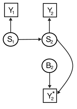
Figure 1: Representation of the multivariate generalized linear geostatistical model (1) as a directed acyclic graph; $S_{1}$ and $S_{2}$ represent prevalences at times $t_{1}$ and $t_{2}>t_{1}$; $B_{2}$ represents bias; $Y_{1}$, $Y_{2}$ and $Y_{2}^{*}$ are observed prevalences from unbiased surveys at times $t_{1}$ and $t_{2}$, and a biased survey at time $t_{2}$, respectively. The target for predictive inference is $S_{2}$.

To extend the model to accommodate multiple surveys taken at possibly different times, some of which may be biased, let $i=1,\dots,r$ denote the index of the survey and $x_{ij}:j=1,\ldots,n_{i}$ the corresponding set of sample locations. We replace the single process $S(x)$ by a set of $r$ processes $S_{i}(x)$ which relate to the true prevalence at different times. We assume that at least one of the surveys is known to be unbiased, define ${\cal B}$ to be the index set of the potentially biased surveys and introduce an additional set of latent Gaussian processes $B_{i}(x):i\in{\cal B}$ to represent the spatially varying biases. Finally, we assume that data from different surveys are generated by conditionally independent univariate GLGMs, with link functions

$$g_{i}(\mu_{ij}/m_{ij}) = \eta_{ij}=d(x_{ij})^{\top}\beta_{1}+S_{i}(x_{ij})+I(i\in{\cal B})[B_{i}(x_{ij})+d(x_{ij})^{\top}\beta_{i}]+Z_{ij},$$ (1)

$$j=1,\ldots,n_{i};i=1,\ldots,r.$$

On the right-hand-side of (1), we assume that the marginal properties of each $S_{i}(x)$ are the same as previously specified for $S(x)$, and add a set of cross-covariance functions, $\mathrm{Cov}\{S_{i}(x),S_{i^{\prime}}(x^{\prime})\}=\sigma^{2}\alpha_{ii^{\prime}}\rho(x,x^{\prime};\phi)$, where $-1<\alpha_{ii^{\prime}}<1$. The parameters $\alpha_{ii^{\prime}}$ capture the temporal correlation between the true prevalence surfaces at different times, hence if surveys $i$ and $i^{\prime}$ are taken at the same time, $S_{i}(x)=S_{i^{\prime}}(x)$ for all $x$ and $\alpha_{ii^{\prime}}=1$. Note that if $r>2$, some combinations of $\alpha_{ii^{\prime}}$ result in a non-positive-definite variance matrix. If $r$ is small, this can be handled by setting the likelihood to zero for all such combinations. When $r$ is large the issue can be avoided by imposing a spatio-temporally continuous parametric structure. This has the incidental benefit of making the model more parsimonious. One such example would be an exponentially decaying cross-covariance structure with $\alpha_{ii^{\prime}}=\exp\{-|t_{i}-t_{i^{\prime}}|/\psi\}$, where $t_{i}$ is the time at which the $i$th survey is taken.

The processes $B_{i}(x)$ in (1) are assumed to be independent, with zero mean and covariance functions $\mathrm{Cov}\{B_{i}(x),B_{i}(x^{\prime})\}=\nu_{i}^{2}\rho(x,x^{\prime};\delta_{i})$.

Finally, the random variables $Z_{ij}$ are again assumed to be mutually independent and Normally distributed with common mean 0 and variances $\tau_{i}^{2}$.

As already noted, when all surveys are taken at the same time, $S_{i}(x)=S_{1}(x)$ for all $i$, which formally corresponds to $\alpha_{ii^{\prime}}=1$ for all $(i,i^{\prime})$. When all surveys are unbiased but are taken at different times, ${\cal B}$ is the empty set and the terms $[B_{i}(x_{ij})+d(x_{ij})^{\top}\beta_{i}]$ in (1) are omitted; formally, this corresponds to $\nu_{i}^{2}=0:i=2,\ldots,r$. If it is appropriate to use different explanatory variables to model the true prevalence and the bias, this is accommodated by setting some elements of the $\beta_{i}$ to zero. The dependence structure of the model is illustrated by the directed acyclic graph in Figure 1 for the special case of two gold-standard surveys conducted at two different times and a biased survey at the second time period. This scenario corresponds to case study analysed in Section 5, where the aim is predictive inference for $S_{2}(x)$. In this case, the potential gains in efficiency by jointly modelling the data from all three surveys stem from the direct links between $S_{2}$ and both $Y_{2}$ and $Y_{2}^{*}$ and the indirect link between $S_{2}$ and $Y_{1}$ via $S_{1}$.

3 Inference

In this section, we focus on the case $r=2$. The generalization to more than two surveys is straightforward. We set $B_{1}(x)=0$, write $B(x)$ in place of $B_{2}(x)$ and write the parameters of this bivariate version of (1) as $\beta=(\beta_{1},\beta_{2})$ and $\theta=(\sigma^{2},\nu^{2},\tau_{1}^{2},\tau_{2}^{2},\phi,\delta,\alpha)$.

3.1 Likelihood

Let $y_{i}=(y_{i1},\ldots,y_{in_{i}})^{\top}$ denote the outcome data from surveys $i=1,2$ and let $D_{i}$ be the $n_{i}$ by $p$ matrix whose $j$th row contains the values $d(x_{ij})=(d_{1}(x_{ij}),\ldots,d_{p}(x_{ij}))^{\top}$. Similarly, let $T_{i}$ denote the vector of the $n_{i}$ values of the linear predictor for survey $i$, hence $T_{i}=D_{i}\{\beta_{1}+I(i=2)\beta_{2}\}+W_{i}$, where $W_{i}=(W_{i1},\ldots,W_{in_{i}})^{\top}$ and

$$W_{ij}=S_{i}(x_{ij})+I(i=2)B(x_{ij})+Z_{ij}.$$ (2)

Now, let $T$ denote the $(n_{1}+n_{2})$-element vector $T=(T_{1}^{\top},T_{2}^{\top})^{\top}$ and $D$ the $(n_{1}+n_{2})$ by $2p$ matrix,

$$D=\left[\begin{array}[]{ll}D_{1}&0\\ D_{2}&D_{2}\end{array}\right].$$ (3)

Also, write $R_{ii^{\prime}}(\phi)$ for the $n_{i}$ by $n_{i^{\prime}}$ matrix with $(h,k)$th element $\rho(x_{ih},x_{i^{\prime}k};\phi)$ and $R_{b}(\delta)$ for the $n_{2}$ by $n_{2}$ matrix with $(h,k)$th element $\rho(x_{2h},x_{2k};\delta)$. Then,

$$T\sim{\rm MVN}(D\beta,V(\theta))$$ (4)

where

$$V(\theta)=\left[\begin{array}[]{ll}\sigma^{2}R_{11}(\phi)+\tau_{1}^{2}I&\sigma^{2}\alpha R_{12}(\phi)\\ \sigma^{2}\alpha R_{21}(\phi)&\sigma^{2}R_{22}(\phi)+\nu^{2}R_{b}(\delta)+\tau_{2}^{2}I\end{array}\right].$$ (5)

The conditional distribution of $Y$ given $T=t$ is a product of independent binomial probability mass functions. We write this as

$$f(y|t)=\prod_{i=1}^{2}\prod_{j=1}^{n_{i}}f(y_{ij}|t_{ij}).$$ (6)

Combining (3), (4), (5) and (6) then gives the likelihood function as the high-dimensional integral

$$L(\beta,\theta)=\int h(t;D\beta,V(\theta))f(y|t)\>dt,$$ (7)

where $h(\cdot|\mu,V)$ is the density function of a multivariate Normal distribution with mean $\mu$ and covariance matrix $V$.

3.2 Conditional simulation

We propose to use Monte Carlo methods to evaluate the high-dimensional integral in (7). These methods require us to simulate from the conditional distribution of the spatial random effect $T$ given the data $Y=y$. Using Bayes’ formula, this conditional density is

$$\pi(t|y)\propto h(t|D\beta,V(\theta))f(y|t).$$ (8)

To simulate from (8), Christensen, Roberts & Sköld (2006) propose a Langevin-Hastings (LH) Markov chain Monte Carlo (MCMC) algorithm. This operates by updating a linear transformation of $T$, chosen to make the components of $T|y$ approximately independent. Christensen, Roberts & Sköld (2006) use a Gaussian approximation to the distribution of $T|y$, with mean $D\beta$ and covariance matrix

$$\tilde{V}=\{V(\theta)+\Lambda(\hat{t})\}^{-1}.$$ (9)

In (9), $\Lambda(t)$ is a diagonal matrix with entries $-\partial^{2}/\partial t_{i}^{2}\log f(y|t)$ and $\hat{t}$ is a typical value of $T$ such as the mode of $f(y|t)$. For the binomial model with logistic link, this gives $\Lambda(\hat{t})=\mathrm{diag}\{y_{i}(1-y_{i}/m_{i})\}$. Christensen, Roberts & Sköld (2006) demonstrate that updating the centred random variable $\tilde{T}=\tilde{V}^{-1/2}(T-D\beta)$ gives better mixing and convergence properties than the analogous MCMC algorithms based on either $T$ or on $\bar{T}=V^{-1/2}(T-D\beta)$, as suggested by Christensen & Waagepetersen (2002).

3.3 Monte Carlo Maximum Likelihood: estimation and spatial prediction

The Monte Carlo Maximum Likelihood (MCML) method (Geyer & Thompson, 1992; Geyer, 1994, 1996, 1999) uses conditional simulations of $T$ given $Y$ to obtain a computationally efficient approximation to the intractable likelihood function. From (7), the likelihood function can be written as

$$L({\beta},{\theta}) = \int h({t}|D{\beta},V({\theta}))f({y}|{t})\>d{t}=\int\frac{h({t}|D{\beta},V({\theta}))f({y}|{t})}{\tilde{f}({y},{t})}\tilde{f}({y},{t})\>d{t}$$ (10)

$$\propto \int\frac{h({t}|D{\beta},V({\theta}))f({y}|{t})}{\tilde{h}({t})f({y}|{t})}\tilde{f}({t}|{y})\>d{t}=E_{\tilde{f}}\left[\frac{h({t}|D{\beta},V({\theta}))}{\tilde{h}({t})}\right].$$

In (10), $\tilde{f}({t},{y})=f({y}|{t})\tilde{h}({t})$, where $\tilde{h}({t})$ is any density function with support in $\mathbb{R}^{n}$, and $E_{\tilde{f}}$ denotes expectation with respect to $\tilde{f}(\cdot|{y})$. MCML estimates are then obtained by maximizing

$$L_{m}({\beta},{\theta})=\frac{1}{m}\sum_{h=1}^{m}\frac{h({t}_{h}|D{\beta},V({\theta}))}{\tilde{h}({t}_{h})},$$ (11)

where ${t}_{1},\ldots,{t}_{m}$ are samples from $\tilde{f}(\cdot|{y})$.

The accuracy of the approximation for a given value of $m$ depends critically on the choice of $\tilde{h}(\cdot)$. A suitable choice is $h({t}_{h}|D{\beta}_{0},V({\theta}_{0}))$, where ${\beta}_{0}$ and ${\theta}_{0}$ are as close as possible to the maximum likelihood estimates, $\hat{{\beta}}$ and $\hat{{\theta}}$. In practice, we embed the maximisation of $L_{m}({\beta},{\theta})$ within the following iterative procedure as suggested in Geyer & Thompson (1992) and Geyer (1994): let $(\hat{\beta}_{1},\hat{\theta}_{1})$ denote the values that maximise $L_{m}({\beta},{\theta})$ using an initial guess at suitable values $({\beta}_{0},{\theta}_{0})$; repeat the maximisation with $(\hat{\beta}_{1},\hat{\theta}_{1})$ replacing $({\beta}_{0},{\theta}_{0})$; continue until convergence.

For the numerical maximization of (11) we use a similar procedure to the one presented in Christensen (2004). Write $V({\theta})=\sigma^{2}V({\psi})$ where $\psi=(\nu^{2}/\sigma^{2},\tau_{1}^{2}/\sigma^{2},\tau_{2}^{2}/\sigma^{2},\phi,\delta,\alpha)^{\top}$ For a given value of ${\psi}$, the first and second derivatives of (11) with respect to ${\beta}$ and $\sigma^{2}$ are analytically tractable and we use an iterative Newton-Raphson algorithm. We then plug into (11) the values $\hat{\beta}(\psi)$ and $\hat{\sigma}(\psi)^{2}$ and maximize with respect to ${\psi}$ using direct numerical optimization with a further re-parameterisation to remove any restrictions on the permissible ranges of the parameters; we use a log-transformation for all elements of $\psi$ except $\alpha$, for which we use $\log\{(1+\alpha)/(1-\alpha)\}$ to correspond to the range $-1<\alpha<1$. We also consider a variety of starting values to guard against false convergence to either a local maximum or an arbitrary point on a plateau of the likelihood surface.

We now consider the prediction of ${T}^{*}=(T(x_{n+1}),\ldots,T(x_{n+q}))^{\top}$ at $q$ additional prediction locations that are not included in any of the prevalence surveys. This requires all relevant explanatory variables to be available at the prediction locations. We include the mutually independent random variables $Z_{ij}$ in (2) as part of our target for prediction. Note that in a linear Gaussian geostatistical model, the $Z_{ij}$ would be conflated with Normally distributed measurement errors, whereas in a GLGM for prevalence survey data the analogue of measurement error is binomial sampling variation and is formally distinguishable from the extra-binomial variation induced by the $Z_{ij}$.

Zhang (2002) gives approximate expressions for the minimum mean square predictor ${\rm E}[{T}^{*}|{y}]$ and its variance using samples from the conditional distribution of $T|y$ generated by conditional simulation. For prediction of non-linear functionals of the prevalence surface, we first use our MCMC algorithm to generate samples $t_{h}:h=1,...,m$ from the conditional distribution of $T|y$, then simulate samples $t_{h}^{*}:h=1,...,m$ directly from the multivariate Normal conditional distribution of ${T}^{*}|T={t}_{h}$. This has expectation

$$D^{*}{\beta}+C^{\top}V^{-1}({t}_{h}-D{\beta}),$$ (12)

where $D^{*}$ is the matrix of covariates at the prediction locations, and covariance matrix

$$V^{*}-C^{\top}V^{-1}C,$$ (13)

where $V^{*}$ is the covariance matrix of ${T}^{*}$ and $C$ is the cross-covariance matrix between ${T}$ and ${T}^{*}$. Finally, we transform the sampled values $t_{h}^{*}$ to predicted prevalences,

$$p_{h}^{*}=g^{-1}({t}_{h}^{*})=(g^{-1}(t_{n+1,h}^{*}),\ldots,g^{-1}(t_{n+q,h}^{*}))^{\top},$$

where $g^{-1}(\cdot)$ is the inverse link function. Typically, the prediction locations will form a fine grid to cover the area of interest, $A$, so as to approximate a set of predicted surfaces, ${\cal P}^{*}=\{p_{h}^{*}(x):x\in A\}$ which can then be summarised according to the needs of each application. For example, we might want to map pointwise means, or selected quantiles, or predictive probabilities of the exceedance of policy-relevant thresholds.

4 Simulation study

We have conducted a simulation study of our proposed methodology with three aims: to show that the parameters in (1) are identifable; to illustrate the finite sample properties of the MCML estimators; and to demonstrate the potential gains in predictive performance that can be obtained by combining data from unbiased and biased surveys.

4.1 Identifiability and finite sample properties

For this part of the simulation study we simulated data from two surveys, the first of which was unbiased, the second biased. We specified the covariance structure of the model to correspond to the MCML estimates that were obtained in the analysis of malaria prevalence data to be reported in Section 5. We also used the same sample sizes as in the malaria application, hence $n_{1}=425$ (to correspond to the second of the two randomised surveys) and $n_{2}=249$ (to correspond to the convenience survey), and the same binomial denominators $m_{ij}$. We did not use covariates but constant means $\beta_{1}$ for the first survey and $\beta_{1}+\beta_{2}$ for the second survey.

Table 1: Estimated means and relative biases (RB) of the MCML estimators for the covariance parameters, and ordered eigenvalues (EV) of their correlation matrix under three scenarios.

		(1)			(2)			(3)
	True value	Mean	RB	EV	Mean	RB	EV	Mean	RB	EV
$\beta_{1}$	1.000	0.997	-0.003	1.677	1.011	0.011	1.677	0.998	-0.002	1.811
$\beta_{2}$	-1.000	-1.011	0.011	1.287	-1.013	0.013	1.425	-0.980	-0.020	1.472
$\sigma^{2}$	2.186	2.132	-0.025	1.173	2.093	-0.042	1.298	2.005	-0.083	1.141
$\tau^{2}$	0.558	0.465	-0.166	0.903	0.476	-0.148	0.840	0.486	-0.130	0.835
$\nu^{2}$	0.672	0.900	0.339	0.772	1.011	0.504	0.715	1.193	0.776	0.806
$\phi$	0.017	0.016	-0.045	0.695	0.016	-0.033	0.577	0.016	-0.085	0.503
$\delta$	0.004	0.005	0.249	0.492	0.006	0.496	0.468	0.008	1.037	0.433

We generated the sampling locations for the unbiased survey as an independent random sample from the uniform distribution in the rectangle $[34.700,34.900]\times[-16.170,-15.880]$. The usefulness of the data from the biased survey may depend on the degree of overlap between the two sets of sampling locations. For this reason we generated the sampling locations for the biased survey from each of three inhomogeneous Poisson processes, with intensity $\lambda(x)=\exp\{-\|x-x_{0}\|/0.02\}$ and $x_{0}$ set to each of the three following locations: $(34.800,-16.025)$, the center of the the rectangle; $(34.700,-16.170)$, the lower left corner of the rectangle; $(34.600,-16.315)$, a point outside the rectangle. Figure 2 shows an example of simulated locations for the biased survey under each of these three scenarios.

Figure 2: example of simulated locations from a biased survey under three different scenarios as defined in Section 4.1; the dashed lines encompass the region within which locations of an unbiased survey are uniformly generated.

For each simulation we computed the mean and relative bias of the MCML estimates of the covariance parameters and the eigenvalues of their correlation matrix, based on 1000 replications of each of the three scenarios. The results are shown in Table 1. The estimates of $\beta_{1}$, $\beta_{2}$, $\sigma^{2}$, $\tau^{2}$ and $\phi$ are approximately unbiased under all three scenarios whereas the estimates of $\nu^{2}$ and $\delta$, which relate to the process $B(x)$, become increasingly biased as the overlap between the two sampled areas decreases. Under all three scenarios, the smallest eigenvalue of the correlation matrix corresponds to about $6\%$ of its total variation as measured by the sum of the eigenvalues. Also, the off-diagonal elements of the correlation matrix, whose entries are never greater than $0.47$ in absolute value, which represents the correlation between the estimates of $\tau^{2}$ and $\phi$ in the third scenario.

The overall conclusion from this part of the simulation study is that all of the model parameters are identifiable, and that the parameter estimates are approximately unbiased provided that there is a substantial overlap in the spatial coverage of the unbiased and biased surveys. This is as expected, because without such overlap the two surveys can only estimate the properties of the sum, $S(x)+B(x)$, in the area covered by the biased survey.

4.2 Quality variation and temporal variation

In this part of the simulation study we focus on predictive performance. Our main objective is to indicate to what extent the inclusion of data from a biased survey can improve predictive inference, under circumstances similar to those that hold in our malaria application. A secondary objective, as suggested by a reviewer, is to demonstrate the unreliability of a naive analysis that ignores bias and temporal variation. We therefore conducted three analyses of each simulated data-set as follows.

• Joint (J). The combined data are analysed using the bivariate GLGM as specified in Section 2.

• First-survey-only (FSO). Only the data from the first, unbiased survey are used.

• “Naive” (N). The data from the two surveys are analysed using a GLGM that does not account for bias or temporal variation.

We consider a quality variation (QV) scenario, in which one survey is unbiased and the other biased, and a temporal variation (TV) scenario, in which both surveys are unbiased but at different times, with predictions required for the first time period.

The following features are common to both scenarios. The processes $S_{i}(x):i=1,2$ have mean $\beta_{1}=1$, variance $\sigma^{2}=1$ and correlation function $\rho(u)=\exp(-u/\phi)$ with $\phi=0.15$. Locations of unbiased surveys are uniformly generated in the unit square centred on $x_{0}=(1/2,1/2)$. Both surveys have the same number of sampling locations, $n_{1}=n_{2}=300$. The binomial denominators at each sampling location are all set equal to 1. Our primary focus is on prediction of prevalence at $x_{0}$ but we also consider estimation of the parameters $\beta_{1}$, $\log\sigma^{2}$ and $\log\phi$ that define the model for the underlying prevalence process $S_{1}(x)$.

In the QV scenario, $S_{1}(x)=S_{2}(x)$ for all $x$ and the process $B_{2}(x)$ has mean $\beta_{2}=-1$ and correlation function $\rho(u)=\exp(-u/\delta)$ with $\delta=0.15$. Locations from the biased survey are generated from a Poisson process with intensity $\lambda(x)=\exp\{-\|x-x_{0}\|/0.15\}$ so that points closer to $x_{0}$ are more likely to be sampled, as might occur when using a convenience sampling strategy and $x_{0}$ is the location of a health-care facility. Finally, we consider four values, $\nu^{2}=0.5,1,2,4$, for the variance of the process $B_{2}(x)$, corresponding to increasingly severe spatial variation in the bias.

In the TV scenario, the cross-correlation function between $S_{1}(x)$ and $S_{2}(x)$ is $\alpha\exp(-u/\phi)$. We consider three values, $\alpha=0.2,0.5,0.8$, to correspond to weak, moderate and strong correlation between the two prevalence surfaces.

The results are summarised in Tables 2 and 3. These show estimates of the root-mean-square-error (RMSE) and coverage of nominal $95\%$ confidence intervals (CIC) for MCML estimates of the parameters $\beta_{1}$, $\log\sigma^{2}$ and $\log\phi$, and for the minimum mean square error predictors of $S_{1}(x_{0})$ and $\beta_{1}+S_{1}(x_{0})$. Each entry is calculated from 1000 independent replicates of the simulation model.

Table 2: Estimated RMSE, bias, SD and $95\%$ CIC for the MCML estimates of $\beta_{1}$, $\log\sigma^{2}$, $\log\phi$, for the minimum mean square error predictor of $S_{1}(x_{0})$ at location $x_{0}$ and $\beta_{1}+S(x_{0})$, under QV scenarios.

Model	Parameter	RMSE				CIC
		$\nu^{2}$				$\nu^{2}$
		0.5	1	2	4	0.5	1	2	4
J		0.37	0.36	0.36	0.36	0.95	0.95	0.95	0.94
FSO	$\beta_{1}$	0.37	0.36	0.35	0.35	0.95	0.95	0.95	0.95
N		0.50	0.52	0.51	0.48	0.82	0.79	0.83	0.77
J		0.94	0.60	0.63	1.33	0.99	0.94	0.95	0.99
FSO	$\log\sigma^{2}$	1.08	1.14	1.04	0.99	0.97	0.97	0.97	0.97
N		0.78	0.49	0.52	0.54	0.99	0.96	0.95	0.91
J		0.84	0.81	0.98	0.95	0.92	0.90	0.92	0.92
FSO	$\log\phi$	1.45	1.42	1.32	1.44	0.94	0.94	0.92	0.94
N		0.69	0.68	0.66	0.70	0.92	0.90	0.88	0.83
J		0.80	0.79	0.88	0.86	0.95	0.95	0.95	0.95
FSO	$S_{1}(x_{0})$	0.91	0.86	0.92	0.85	0.95	0.95	0.95	0.94
N		0.93	0.96	1.13	1.21	0.80	0.80	0.77	0.76
J		0.72	0.73	0.82	0.83	0.95	0.95	0.95	0.95
FSO	$\beta_{1}+S_{1}(x_{0})$	0.83	0.80	0.84	0.81	0.95	0.94	0.95	0.94
N		1.10	1.15	1.33	1.35	0.78	0.78	0.75	0.74

Table 3: Estimated RMSE, bias, SD and $95\%$ CIC for the MCML estimates of $\beta_{1}$, $\log\sigma^{2}$, $\log\phi$, for the minimum mean square error predictor of $S_{1}(x_{0})$ at location $x_{0}$ and $\beta_{1}+S(x_{0})$, under TV scenarios.

Model	Parameter	RMSE			CIC
		$\alpha$			$\alpha$
		0.2	0.5	0.8	0.2	0.5	0.8
J		0.35	0.35	0.35	0.95	0.93	0.94
FSO	$\beta_{1}$	0.36	0.36	0.35	0.94	0.93	0.93
N		0.63	0.63	0.64	0.29	0.38	0.42
J		0.60	0.68	0.69	0.94	0.94	0.93
FSO	$\log\sigma^{2}$	1.04	1.46	1.47	0.97	0.96	0.96
N		1.18	0.95	0.87	0.91	0.92	0.95
J		0.93	0.92	0.91	0.91	0.93	0.93
FSO	$\log\phi$	1.47	1.56	1.75	0.92	0.93	0.94
N		1.32	1.09	1.02	0.92	0.94	0.94
J		1.37	1.30	1.28	0.95	0.95	0.94
FSO	$S_{1}(x_{0})$	1.37	1.30	1.31	0.94	0.93	0.92
N		1.39	1.32	1.28	0.87	0.91	0.92
J		1.34	1.28	1.26	0.96	0.96	0.94
FSO	$\beta_{1}+S_{1}(x_{0})$	1.35	1.27	1.27	0.95	0.95	0.94
N		1.50	1.39	1.36	0.86	0.90	0.91

Overall, J outperforms FSO, which in turn outperforms N. Under the QV scenario, the main benefits of J are in the prediction of $S_{1}(x_{0})$ for values of $\nu^{2}$ smaller than $4$. The N approach yields much higher values of RMSE for the estimates of $\beta_{1}$, $S_{1}(x_{0})$ and $\beta_{1}+S_{1}(x_{0})$ and very poor CIC. Under the TV scenario, the biggest gains achieved by J over FSO are in estimating the parameters $\log\sigma^{2}$ and $\log\phi$. Both J and FSO perform similarly with respect to prediction of $S_{1}(x_{0})$ and $\beta_{1}+S_{1}(x_{0})$. The N approach, which in this scenario consists of combining the data under the assumption that $S_{1}(x)=S_{2}(x)$ for all $x$, i.e. $\alpha=1$, has the worst performance.

5 Application: malaria prevalence mapping

In this Section, we use our proposed methodology to construct malaria prevalence maps for an area of Malawi by combining information from three surveys. All three surveys were directed at the same target population, covering a 400 square km area within Chikhwawa District, Southern Malawi. Two of the surveys were “rolling” Malaria Indicator Surveys (MIS) (Roca-Feltrer, Lalloo, Phiri & Terlouw, 2012), that used two different practical strategies to obtain random, and therefore unbiased, samples from the population at risk. The third was a facility-based survey that used a convenience sampling strategy, in which recruitment took place at a central child-vaccination clinic at the main hospital in the centre of the study area. We refer to this as the Easy Access Group (EAG) study.

5.1 Data

Figure 3: Sampled locations for (a) rMIS, (b) eMIS and (c) EAG. Coordinates are of individual houses for rMIS and eMIS, and of the villages for EAG; in (c), the radius of each circle is proportional to the number of the sampled households from the respective village and the black solid point corresponds to CDH village. The light blue lines represent waterways, with the thicker line corresponding to Shire river.

Two population-level continuous malaria indicator surveys were conducted over the period May 2010 to April 2012. Both surveys recruited children aged less than five years in a sample of 50 village communities in order to monitor the malaria intervention coverage and childhood burden of malaria in a designated area containing the sampled villages, which was chosen to represent the catchment area of the Chikhwawa District Hospital (CDH). The two surveys differed in the sampling strategy used, as described below. We refer to these two surveys as the rMIS, covering the period May 2010 to April 2011 and the eMIS, covering the period May 2011 to April 2012. Throughout the two-year period seven or eight villages were randomly selected per month so as to sample all 50 villages twice yearly, once during the high-transmission season and once during the low-transmission season. Within sampled villages, selection of households was as follows. In the rMIS, households were randomly selected within each village from a list of households, with sampling probability proportional to village population size, based on a population enumeration exercise. In the eMIS, a more economical “spin-the-bottle” method was used to identify a random set of households within villages. A bottle was placed in the center of a village and used to select random directions. A virtual line was drawn in each chosen direction to the border of the village, the households that intersected this line were counted, and from these a random household number was chosen as the starting point. The number of houses selected within each village was proportional to the estimated village population size. Figures 3 (a)-(b) show the sampled locations for the rMIS and the eMIS.

The third survey is a continuous facility-based MIS in children attending the immunization clinic at the CDH, conducted from May 2011 to April 2012. The objective of this study was to determine if estimates of uptake of control interventions and the burden of malaria from convenience sampling were comparable to those from a randomised MIS conducted within the same catchment area of CDH. Children from 3 months of age who attended the vaccination clinic, and any accompanying sibling below 5 years, were recruited. Between 30 and 50 children were recruited per month. Village of origin was extracted by direct questioning. If the village was not one of the 50 eMIS/rMIS villages for which the location was already known, its coordinates were determined retrospectively. The results for villages within 15km of CDH were extracted to make the catchment area of the EAG comparable to that of the rMIS and eMIS. Malaria control efforts by the national control program during the first period included a district-wide household indoor residual spraying campaign between February and April 2011. Practical difficulties resulted in this campaign being conducted at the end of the rainy season rather than, as would have been ideal, before the start of the rainy season. This will have reduced its potential impact. Insecticide-treated net control efforts were stable over the three months of the campaign, with distribution to women attending antenatal clinics and mother and child clinics.

5.2 Results

The response from each child was a binary indicator of the outcome of a rapid diagnostic test (RDT) used to test for the presence of malaria from a finger-prick blood sample. Six explanatory variables were considered, as defined in Table 4. Socio-Economic-Status (SES), an indicator of household wealth taking discrete values from 1 (poor) to 5 (wealthy), was derived by an application of principal component analysis as discussed in Vyas & Kumuranayake (2006).

Table 4: Explanatory variables used in the analysis of the Chikhwawa malaria prevalence surveys

1	intercept
2	at least one treated bed-net in the household (yes/no)
3	indoor residual spraying in the past two months (yes/no)
4	high-transmission season (January-June/July-December)
5	distance from the closest waterway (km)
6	Socio-Economic-Status (SES, 1 to 5)

It was thought that health facility utilization might be associated with SES as previously observed in Gahutu et al. (2011), where children with relatively high SES were more likely to attend a CDH. Table 6 shows the average SES observed in each of our three surveys. Enrolled children in the EAG study show a higher average SES then those in the two other surveys. Additionally, Table 6 shows that the relationship between SES and the distribution of the number of RDT positive results per household differs between the two gold-standard surveys and the convenience survey. We therefore allowed SES to have a direct effect on the spatially structured bias of the EAG survey in addition to its possible association with prevalence.

Table 5: Mean and standard deviation (SD) of SES in the three surveys.

	SES
	rMIS	eMIS	EAG
Mean	2.76	2.50	3.45
SD	1.45	1.37	1.39

Table 6: Distribution (percentage) of the number of positive RDTs per household for each value of SES, in the convenience survey (EAG, left-columns) and in the gold-standard surveys (rMIS and eMIS, right columns)

		SES (EAG)					SES (rMIS and eMIS)
		1	2	3	4	5	1	2	3	4	5
	0	75.76	80.56	77.50	79.10	89.04	54.58	63.09	71.72	73.29	83.74
RDT	1	21.21	19.44	20.00	20.90	10.96	40.49	33.56	25.25	22.60	15.45
positives	2	3.03	0.00	2.50	0.00	0.00	4.58	3.35	3.03	3.42	0.81
	3	0.00	0.00	0.00	0.00	0.00	0.35	0.00	0.00	0.69	0.00

Table 7: Monte Carlo maximum likelihood estimates and $95\%$ confidence intervals.

Term	Estimate	95% confidence interval
$\beta_{1}$	-0.272	(-1.382, 0.862)
$\beta_{2}$	-0.439	(-0.623, -0.277)
$\beta_{3}$	-0.399	(-0.621, -0.189)
$\beta_{4}$	0.415	(0.206, 0.598)
$\beta_{5}$	-0.373	(-0.970, 0.116)
$\beta_{6}$	-0.151	(-0.233, -0.072)
$\beta_{7}$	-0.096	(-0.222, 0.021)
$\sigma^{2}$	2.186	(0.955, 3.155)
$\tau^{2}$	0.558	(0.089, 1.231)
$\nu^{2}$	0.672	(0.525, 0.802)
$\alpha$	0.859	(0.483, 0.924)
$\phi$	0.017	(0.006, 0.032)
$\delta$	0.004	(0.001, 0.025)

The resulting model for the combined data therefore included seven regression parameters, $\beta_{1},\beta_{2},...,\beta_{7}$. Let $\beta^{\top}=(\beta_{1},\dots,\beta_{6})$ and denote by $d(x_{ij})$ the vector of covariates associated with location $x_{ij}$. Use $i=1,2,3$ to denote rMIS, eMIS and EAG, respectively. Then, the linear predictor is

$$\eta_{ij} = d(x_{ij})^{\top}\beta+S_{i}(x_{ij})+I(i=3)[B(x_{ij})+\beta_{7}\text{SES}_{ij}]+Z_{ij},$$

$$i=1,\ldots,3;j=1,\ldots,n_{i},$$

where $n_{1}=475$, $n_{2}=425$ and $n_{3}=249$. Note that in the joint model for $S_{1}(x)$, $S_{2}(x)$ and $S_{3}(x)$, $\alpha_{23}=1$ because the EAG study took place over the same period as the eMIS. We therefore use $\alpha$ to denote $\alpha_{12}$ and set $S_{3}(x)=S_{2}(x)$. We also assume equal variances $\tau^{2}$ for the nugget term $Z$ across all three surveys. Finally, we define $\mathrm{Cov}\{S_{1}(x),S_{2}(x^{\prime})\}=\sigma^{2}\alpha\exp\{-\|x-x^{\prime}\|/\phi)$ where $\sigma^{2}>0$, $\phi>0$ and $-1<\alpha<1$.

Table 7 shows the Monte Carlo maximum likelihood estimates of the model parameters together with $95\%$ confidence intervals. Each evaluation of the log-likelihood used $5000$ simulated values, obtained by conditional simulation of $110000$ values and sampling every $20$th realization after discarding a burn-in of $10000$ values. Figure 4 shows two diagnostic plots for the average random effect: convergence of the MCMC algorithm appears to be satisfactory.

The confidence intervals in Table 7 were calculated using the following parametric bootstrap procedure.

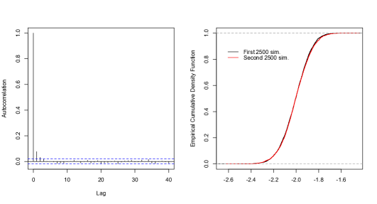
Figure 4: Diagnostic plots for the convergence of the posterior average of the random effect. Left panel: correlogram of the 5000 simulated values. Right panel: empirical cumulative density function for the first (black line) and second (red line) 2500 simulated values.

Using the parameter estimates in Table 7 we simulated $1000$ data-sets from the model, applied to each simulated data set the Monte Carlo maximum likelihood method with $5000$ conditional simulations, and computed the empirical quantiles of the $1000$ resulting estimates of each parameter. Although this procedure introduces additional Monte Carlo error, it allows us to compute confidence intervals without relying on questionable Normal approximations for the distribution of the Monte Carlo maximum likelihood estimates.

From Table 7, we see that the ownership of at least one treated bed net, the presence of residual indoor spraying and an increase in SES are all associated with a reduction in the prevalence of a positive RDT. The distance from the closest waterway is not significant, although the sign of the regression coefficient suggests that prevalence decreases with increasing distance. The period January to June, which is known to be a period of high malaria transmission, is associated with a significant increase in prevalence, by an estimated factor of $\exp(0.415)\approx 1.51$.

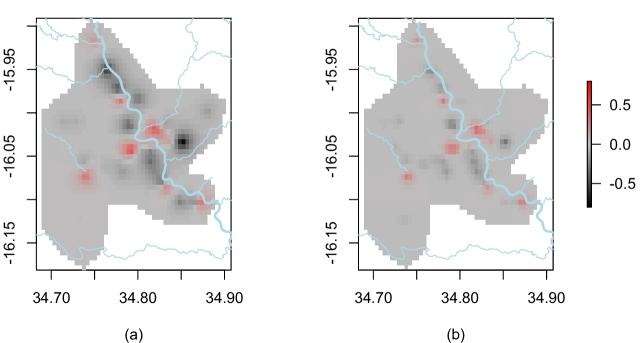
Figure 5: Predicted bias surface $B(x)$ (a) without the interaction term of SES and (b) including the effect of SES on the spatial bias.

The regression coefficient $\beta_{7}$, which represents the additional effect of SES on the bias of the EAG data, is not significant, but its inclusion nevertheless makes a noticeable difference to the predicted bias surface. Figures 5(a) and 5(b) show the minimum mean square error predictions of the bias with and without including the regression on SES.

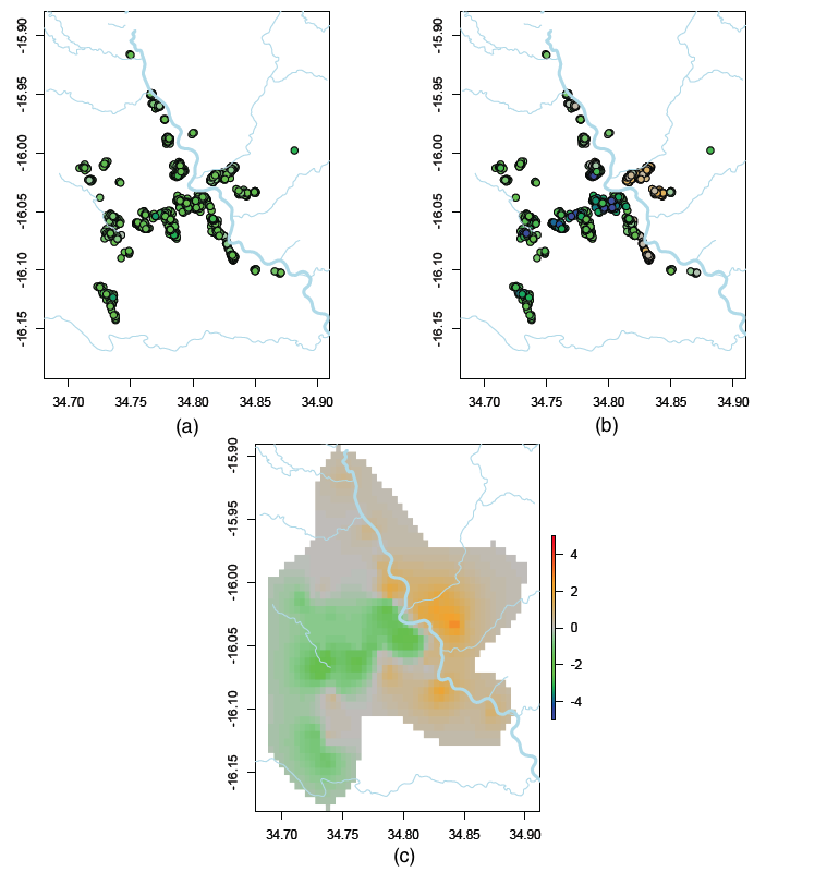
Figure 6: Predictions of (a) $d(x_{2j})^{\top}\beta$ and (b) $d(x_{2j})^{\top}\beta+S_{2}(x_{2j})$ at observed locations; (c) predicted surface of the unexplained spatial variation $S_{2}(x)$. The same colour scale has been used for the point predictions.

The estimate $\hat{\alpha}=0.859$, albeit with a wide confidence interval, indicates a strong correlation between prevalences in the two sampling periods, 2010-2011 and 2011-2012.

Figures 6a and b show the contributions of the linear regression and of the unexplained spatial variation to the predicted log-odds of prevalence at each of the observed locations. Figure 6c shows the unexplained component, $\hat{S}(x)$, of the predicted prevalence as a spatially continuous surface. The clear and substantial difference between adjacent areas to the east and west of the river Shire strongly suggests the existence of one, or more, social or environmental risk-factors that are not captured by the available explanatory variables.

Figure 7 shows pairwise scatter plots to compare the prediction standard deviations for $S_{2}(x)$ at the sampling locations. Figure 7 (a) shows that analysing rMIS and eMIS data in the joint model for temporal variation results in substantially better precision than using only the eMIS; Figures 7 (c) and (d) show the further, but more modest, gains resulting from addition of the data from the EAG; in contrast, Figure 7 (b) suggests little or no benefit from adding the EAG data to the eMIS data, with predictive standard deviations decreasing at some locations but increasing at others.

Figure 7: Scatter plots of the prediction standard errors for $S_{2}(x)$ at sampled locations $x$, using models fitted to the data from: (a) eMIS against eMIS and rMIS; (b) eMIS against eMIS and EAG; (c) eMIS, rMIS and EAG against eMIS; (d) eMIS, rMIS and EAG against eMIS and rMIS.. The solid line represents the identity line.

6 Discussion

We have developed a class of multivariate GLGMs for the combined data from multiple spatially referenced surveys, and associated Monte Carlo methods for maximum likelihood estimation and spatial prediction within the proposed class of models.

The model as defined by (1) is the minimally parameterised model that captures the essential features of our motivating application: variation in data-quality arising from non-randomised sampling; variation in prevalence over time; binomial and extra-binomial sampling variation. We have shown that all of the model parameters are identifiable from surveys of comparable size to the ones available to us for the application. If substantially larger data-sets were available, it would be of interest to extend the model in various ways, for example by relaxing the assumption of common parameters for the prevalence surfaces $S_{i}(x)$ at different times or by allowing cross-correlation between the $S_{i}(x)$ and their paired bias surfaces $B_{i}(x)$. Additionally, if a large number of surveys were conducted at irregularly spaced time-points within partly overlapping time periods, the use of a structured spatio-temporally continuous process $S(x,t)$, as mentioned in Section 2, would be more appealing than a discrete set of processes $S_{i}(x)$ at specific times $t_{i}$.

The Monte Carlo maximum likelihood estimation procedure is computationally intensive, primarily because of the need to use parametric bootstrapping to compute standard errors reliably. For this reason, we are currently developing a much faster Monte Carlo method for approximate evaluation of the likelihood function.

In our application to malaria prevalence surveys, we combined data from three surveys, two of which were unbiased and conducted in two consecutive years,whilst the third was a potentially biased convenience survey conducted over the same time-period as the second unbiased survey. We obtained substantial gains in the precision of spatial predictions by combining the data from the two unbiased surveys and further, but smaller, gains from combining the data from all three surveys.

One of the limitations of our approach is that it assumes that at least one of the available surveys represents an unbiased gold-standard. This is a reasonable assumption when, as in our application, at least one of the surveys uses a properly randomised sampling scheme. When we cannot assume that one of the surveys is unbiased by design, it is difficult to see how any method could deliver reliable predictions without additional assumptions that would be difficult or impossible to validate empirically.

The problem that we have addressed in this paper is related to, but distinct from, the problem of preferential sampling as formulated in Diggle et al. (2010). In both settings, the goal is to predict the realisation of a latent spatial process $S(x)$ using data obtained by a potentially biased sampling scheme. In preferential sampling, the bias arises from a direct relationship between the value of $S(x)$ and the probability that the location $x$ will be sampled. In the present paper, the bias is a function of the location $x$ itself, rather than of the value of $S(x)$. In the context of disease prevalence mapping, a further distinction is between properties of a location and properties of a person who happens to live at that location. Thus, in our application a relationship between a child’s location and the likelihood that they would present at the CDH would not, in itself, result in bias. Rather, the bias surface $B(x)$ allows for the possibility that the sub-population of children who present at the CDH differs from the general population with respect to their exposure to unmeasured risk-factors for malaria.

Our approach is of potentially wide application to disease monitoring and control in low-resource settings, where registry data are typically not available. The ability to combine data from surveys that vary in their level of bias and timing can inform more accurate, local-area burden maps, allowing for improved risk stratification of high burden areas and identification of transmission hot-spots. For example, although substantial progress has been made over the past decade with malaria control by homogeneous scaling up of interventions at national level, it is increasingly recognized by funders and policy makers that a more targeted approach focused on high-burden areas or hot-spots may be more cost-effective. Furthermore, apart from its potential to optimize the use of available data, our approach can also inform improved prospective data collection, by using the fitted model in simulation studies to identify efficient prospective hybrid sampling approaches that combine convenience and random sampling strategies in ways that acknowledge and exploit spatial and/or temporal heterogeneity as revealed by analyses of the kind described in Section 5.

In conclusion, our proposed approach provides a way of making use of mixed source prevalence data to improve estimates of spatial predictions. These are urgently needed to support control programmes and develop more accurate local spatio-temporal risk stratification maps that can inform more targeted control efforts. Malaria is one of a number of diseases that bring a high public health burden in low-resource settings, whilst exhibiting highly heterogeneous distributions across space and time. Control of such diseases needs methods of continuous monitoring of prevalence and evaluation of control measures that make the best possible use of limited resources, and will therefore benefit greatly from the ability to combine national household surveys with more local convenience sampling strategies without compromising the validity of the resulting prevalence estimates.

Funding

Emanuele Giorgi holds an ESRC-NWDTC funded Ph.D. studentship. Dr Sanie Sesay holds an MCDC funded Ph.D. studentship. Dr Dianne Terlouw acknowledges support from the ACT consortium for the presented household prevalence surveys from Malawi. Prof Peter Diggle is supported by the UK Medical Research Council (grant number G0902153).

References

- Christensen (2004) Christensen, O. F. (2004). Monte Carlo maximum likelihood in model-based geostatistics. Journal of Computational and Graphical Statistics 13, 702–718.
- Christensen et al. (2006) Christensen, O. F., Roberts, G. O. & Sköld, M. (2006). Robust Markov chain Monte Carlo methods for spatial generalized linear mixed models. Journal of Computational and Graphical Statistics 15, 1–17.
- Christensen & Waagepetersen (2002) Christensen, O. F. & Waagepetersen, R. P. (2002). Bayesian prediction of spatial count data using generalized linear mixed models. Biometrics 58, 280–286.
- Crainiceanu et al. (2008) Crainiceanu, C., Diggle, P. & Rowlingson, B. (2008). Bivariate modelling and prediction of spatial variation in Loa loa prevalence in tropical Africa (with discussion). Journal of the American Statistical Association 103, 21–43.
- Diggle et al. (2010) Diggle, P. J., Menezes, R. & Su, T. (2010). Geostatistical inference under preferential sampling. Journal of the Royal Statistical Society, Series C 59, 191–232.
- Elliot & Davis (2005) Elliot, M. R. & Davis, W. W. (2005). Obtaning risk factor prevalence estimates in small areas: combining data from two surveys. Journal of the Royal Statistical Society, Series C 54, 595–609.
- Gahutu et al. (2011) Gahutu, J.-B., Steininger, C., Shyirambere, C., Zeile, I., Cwinya-Ay, N., Danquah, I., Larsen, C., Eggelte, T., Uwimana, A., Karema, C., Musemakweri, A., Harms, G. & Mockenhaupt, F. (2011). Prevalence and risk factors of malaria among children in southern highland rwanda. Malaria Journal 10, 134.
- Geyer (1994) Geyer, C. J. (1994). On the convergence of Monte Carlo maximum likelihood calculations. Journal of the Royal Statistical Society, Series B 56, 261–274.
- Geyer (1996) Geyer, C. J. (1996). Estimation and optimization of functions. In Markov Chain Monte Carlo in Practice, W. Gilks, S. Richardson & D. Spiegelhalter, eds. London: Chapman and Hall, pp. 241––258.
- Geyer (1999) Geyer, C. J. (1999). Likelihood inference for spatial point processes. In Stochastic Geometry, Likelihood and Computation, O. E. Barndorff-Nielsen, W. S.Kendall & M. N. M. van Lieshout, eds. Boca Raton, FL: Chapman and Hall/CRC, pp. 79––140.
- Geyer & Thompson (1992) Geyer, C. J. & Thompson, E. A. (1992). Constrained Monte Carlo maximum likelihood for dependent data. Journal of the Royal Statistical Society, Series B 54, 657–699.
- Hedt & Pagano (2011) Hedt, B. L. & Pagano, M. (2011). Health indicators: Eliminating bias from convenience sampling estimator. Statistics in Medicine 30, 560–568.
- Lohr & Rao (2006) Lohr, S. L. & Rao, J. N. K. (2006). Estimation in multiple-frame surveys. Journal of the American Statistical Association 101, 1019–1030.
- Manzi et al. (2011) Manzi, G., Spiegelhalter, D. J., Turner, R. M., Flowers, J. & Thompson, S. G. (2011). Modelling bias in combining small area prevalence estimates from multiple sruveys. Journal of the Royal Statistical Society, Series A 174, 31–50.
- McCullagh & Nelder (1989) McCullagh, P. & Nelder, J. (1989). Generalized Linear Models. Chapman and Hall, London, 2nd ed.
- Moriarity & Scheuren (2001) Moriarity, C. & Scheuren, F. (2001). Statistical matching: A paradigm for assesing the uncertainty in the procedure. Journal of Official Statistics 17, 407–422.
- R Core Team (2012) R Core Team (2012). R: A Language and Environment for Statistical Computing. R Foundation for Statistical Computing, Vienna, Austria. ISBN 3-900051-07-0.
- Raghunathan et al. (2007) Raghunathan, T. E., Xie, D., Schenker, N. & Parsons, V. L. (2007). Combining information from two surveys to estimate county-level prevalence rates of cancer risk factors and screening. Journal of the American Statistical Association 102, 474–486.
- Roca-Feltrer et al. (2012) Roca-Feltrer, A., Lalloo, D., Phiri, K. & Terlouw, D. J. (2012). Rolling Malaria Indicator Surveys (rMIS): a potential district-level malaria monitoring and evaluation (M&E) tool for programme managers. American Journal of Tropical Medicine and Hygiene 86, 96–98.
- Turner et al. (2009) Turner, R. M., Spiegelhalter, D. J., Smith, G. C. S. & Thompson, S. G. (2009). Bias modelling in evidence synthesis. Journal of the Royal Statistical Society, Series A 172, 21–47.
- Vyas & Kumuranayake (2006) Vyas, S. & Kumuranayake, L. (2006). Constructing socio-economic status indices: how to use principal component analysis. Health Policy Plan 21, 459–468.
- Wanji et al. (2012) Wanji, S., Akotshi, D., Kankou, J., Nigo, M., Tepage, F., Ukety, T., Diggle, P. & Remme, J. (2012). The validation of the rapid assessment procedures for loiasis (RAPLOA) in the Democratic Republic of Congo: health policy implications. Parasites and Vectors 5, 25 doi:10.1186/1756--3305--5--25.
- Zhang (2002) Zhang, H. (2002). On estimation and prediction for spatial generalized linear mixed models. Biometrics 58, 129–136.