On the Relationship between Discrete and Continuous Energy Spectra of SU($N$) Supermembrane Matrix Model

It has been known that SU($N$) supermembrane matrix model has continuous energy spectrum, and it has also been conjectured that it has a normalizable energy eigenstate. Assuming that there exists a normalizable energy eigenstate for each $N$, we show that there exists a branch of continuous energy spectrum for each partition of $N$.

1 Introduction

The SU($N$) supermembrane matrix quantum mechanics, which is obtained from the dimensional reduction of $(9+1)\,$D SYM to $(0+1)\,$D, describes low energy physics of $N$ D0-branes in type IIA string theory, gives a regularization of M2-brane effective action in M-theory[1], and is expected to describe discrete light cone quantized M-theory[2, 3].

To know more about string theory and M-theory, it is important to study this system quantum mechanically, especially to study the structure of energy spectrum. In [4], it has been shown that this system has continuous spectrum. Therefore most of eigenstates are expected to be nonnormalizable. However this fact does not forbid existence of normalizable energy eigenstates, and indeed the following conjecture has been made: There exists a unique normalizable zero energy eigenstate. This conjecture is natural in the viewpoint of D0-brane physics: if we uplift 10D type IIA string theory to 11D M-theory, a single D0-brane is regarded as a Kaluza-Klein(KK) mode of one momentum unit along 11-th direction. $N$ D0-branes correspond to $N$ KK modes of one momentum unit, and a single KK mode of $N$ times the momentum unit can be given as a threshold bound state of $N$ KK modes of one momentum unit.

Then we are naturally led to the following description of the continuous spectrum: Let us partition $N$ into positive integers $N_{\mu}$: $N=\sum_{\mu=1}^{n_{b}}N_{\mu}$. $N$ D0-branes can form $n_{b}$ bound states which consist of $N_{\mu}$ D0-branes respectively. This can be regarded as a $n_{b}$ particle state, and if those particles are far apart from each other they behave as free particles. Therefore it gives a branch of continuous spectrum.

The purpose of this paper is to make the above description of the continuous spectrum more rigorous. We do not inquire into the spectrum of normalizable states, but just assume that there exists a normalizable energy eigenstate in the SU($N$) quantum mechanics for each $N$, and the wavefunctions of those normalizable states decay sufficiently fast at infinity. Extending the argument given in [4], we shall show that for each partition of $N$ there is a branch of continuous spectrum. The argument in [4] corresponds to the case where $N_{\mu}=1$ for any $\mu$.

This paper is organized as follows. After summarizing notation in Section 2, we shall show in Section 3 that using normalizable energy eigenstates $\psi_{(\mu)}$ of energy $E_{(\mu)}$ taken from SU($N_{\mu}$) subsystems, we can construct a smooth gauge invariant function $\psi_{t,L}$ with two parameters $t$ and $L$ which has the following property:

For any $E\in[0,\infty)$ and $\epsilon>0$, there exist $L_{0}$ and $t_{0}(L)$ such that

$$\forall L>L_{0}~{}~{}\text{and}~{}~{}\forall t>t_{0}(L),\quad||\psi_{t,L}||=1~{}\text{and}~{}\Big{|}\Big{|}\Big{(}H-E-\sum_{\mu}E_{(\mu)}\Big{)}\psi_{t,L}\Big{|}\Big{|}<\epsilon.$$

where $H$ is the Hamiltonian of the SU($N$) quantum mechanics. Roughly speaking, $L$ restricts the size of the normalizable bound states $\psi_{(\mu)}$, and $t$ is the distances between them. This fact means that there are branches of continuous energy spectrum of ranges $\Big{[}\sum_{\mu}E_{(\mu)},\infty\Big{)}$.

In Section 4, in order to ensure that the above branches are independent of each other, we shall show that inner products of $\psi_{t,L}$ corresponding to different partitions of $N$, or corresponding to different eigenstates of SU($N_{\mu}$) subsystems, can be taken arbitrarily small i.e.

For any $\epsilon>0$, there exist $L_{0}$ and $t_{0}(L,L^{\prime})$ such that

$$\forall L,L^{\prime}>L_{0}~{}~{}\text{and}~{}~{}\forall t,t^{\prime}>t_{0}(L,L^{\prime}),\quad\big{|}\left\langle\psi_{t,L},\psi^{\prime}_{t^{\prime},L^{\prime}}\right\rangle\big{|}<\epsilon,$$

if $\psi_{t,L}$ and $\psi^{\prime}_{t^{\prime},L^{\prime}}$ correspond to different partitions of $N$ or different eigenstates of SU($N_{\mu}$) subsystems.

Section 5 contains some discussions. In Appendix A we collect information on group theory necessary for the analysis. In Appendix B we define some auxiliary functions used for defining $\psi_{t,L}$, and discuss some of their properties. In Appendix C we discuss smoothness of eigenvalues and matrices used for defining $\psi_{t,L}$.

2 Preliminaries

In this section we first have a quick review of the setup used in [4], and then we extend it to the one suitable for our purpose.

2.1 Diagonally gauge fixed description of SU($N$) supermembrane matrix model

The SU($N$) supermembrane matrix quantum mechanics is described by Grassmann even hermitian traceless matrices $X^{I}$ and $X^{9}$, and Grassmann odd hermitian traceless matrices $\theta_{\alpha}$, where $(I,9)=(1,\dots,8,9)$ is an SO(9) vector index, and $\alpha=1,2,\dots,16$ is an SO(9) spinor index. Gamma matrices $(\gamma^{I})^{\alpha\beta}$ and $(\gamma^{9})^{\alpha\beta}$ are real and symmetric, satisfying

$$\{\gamma^{I},\gamma^{J}\}=2\delta^{IJ},\quad\{\gamma^{I},\gamma^{9}\}=0,\quad(\gamma^{9})^{2}=1.$$ (2.1)

Using the basis which diagonalizes $\gamma^{9}$, $\alpha$ splits into $\alpha^{\prime}$ and $\alpha^{\prime\prime}$ as follows:

$$\gamma^{9}=\begin{pmatrix}\delta_{\alpha^{\prime}\beta^{\prime}}&\\ &-\delta_{\alpha^{\prime\prime}\beta^{\prime\prime}}\end{pmatrix},\quad\gamma^{I}=\begin{pmatrix}&(\gamma^{I})_{\alpha^{\prime}\beta^{\prime\prime}}\\ (\gamma^{I})_{\alpha^{\prime\prime}\beta^{\prime}}&\end{pmatrix}.$$ (2.2)

We describe SU($N$) Lie algebra with a Cartan-Weyl basis $\{h_{m},E_{ij};\;m=1,2,\dots,N-1,\;i,j=1,2,\dots,N,\;i\not\neq j\}$ (For notation about SU($N$) see Appendix A). $\theta_{\alpha}$ are expanded as

$$\theta_{\alpha}=\theta_{\alpha}^{m}h_{m}+\theta_{\alpha}^{(ij)}E_{ij}.$$ (2.3)

Here and in the following, $(i,j)$ component of $\theta_{\alpha}$ is denoted by $\theta_{\alpha}^{(ij)}$. Unless otherwise stated, when a pair of indices $(ij)$ is repeated it implies summation $\sum_{i,j,i\not\neq j}$. Independent degrees of freedom of the diagonal components $\theta_{\alpha}^{(ii)}$ are given by $\theta_{\alpha}^{m}$. The nonzero anticommutation relations of $\theta_{\alpha}$ are

$$\{\theta_{\alpha}^{m},\theta_{\beta}^{n}\}=\delta_{\alpha\beta}\delta^{mn},\quad\{\theta_{\alpha}^{(ij)},\theta_{\beta}^{(kl)}\}=\delta_{\alpha\beta}\delta^{il}\delta^{jk}.$$ (2.4)

Note that $(\theta_{\alpha}^{(ij)})^{\dagger}=\theta_{\alpha}^{(ji)}$. $X^{9}$ and $X^{I}$, and their conjugate momenta $\Pi^{9}$ and $\Pi^{I}$ can be expanded analogously, and their nonzero commutation relations are

$$[X^{Im},\Pi^{J}_{n}]=i\delta^{IJ}\delta^{mn},\quad[X^{I(ij)},\Pi^{J}_{(kl)}]=i\delta^{IJ}\delta^{i}_{k}\delta^{j}_{l},$$ (2.5)

and analogously for $X^{9}$ and $\Pi^{9}$. Then the momenta are regarded as $\Pi_{m}^{I}=-i\frac{\partial}{\partial X^{Im}}$, $\Pi_{(ij)}^{I}=-i\frac{\partial}{\partial X^{I(ij)}}$, and analogously for $\Pi^{9}$.

SU($N$) gauge invariant Hamiltonian $H$ of this quantum mechanics is

$$H = \text{tr}\Big{[}\frac{1}{2}\Pi^{I}\Pi^{I}+\frac{1}{2}\Pi^{9}\Pi^{9}-\frac{1}{4}[X^{I},X^{J}]^{2}-\frac{1}{2}[X^{9},X^{I}]^{2}$$ (2.6)

$$+\frac{1}{2}\theta\gamma^{9}[X^{9},\theta]+\frac{1}{2}\theta\gamma^{I}[X^{I},\theta]\Big{]}.$$

Generators of the gauge transformation $G$ is decomposed into $X^{9}$ independent part $\hat{G}$ and $X^{9}$ dependent part $G^{9}$: $G=\hat{G}+G^{9}$, where

$$G^{9}_{m} = (h_{m}^{i}-h_{m}^{j})[iX^{9(ij)}\Pi^{9}_{(ij)}],$$ (2.7)

$$G^{9}_{(ij)} = (h_{m}^{i}-h_{m}^{j})[iX^{9(ji)}\Pi^{9}_{m}-iX^{9m}\Pi^{9}_{(ij)}]$$ (2.8)

$$+i\sum_{k\not\neq i,j}[X^{9(jk)}\Pi^{9}_{(ik)}-X^{9(ki)}\Pi^{9}_{(kj)}],$$

$$\hat{G}_{m} = (h_{m}^{i}-h_{m}^{j})[iX^{I(ij)}\Pi^{I}_{(ij)}+\frac{1}{2}\theta_{\alpha}^{(ij)}\theta_{\alpha}^{(ji)}],$$ (2.9)

$$\hat{G}_{(ij)} = (h_{m}^{i}-h_{m}^{j})[iX^{I(ji)}\Pi^{I}_{m}-iX^{Im}\Pi^{I}_{(ij)}+\theta_{\alpha}^{(ji)}\theta_{\alpha}^{m}]$$ (2.10)

$$+i\sum_{k\not\neq i,j}[X^{I(jk)}\Pi^{I}_{(ik)}-X^{I(ki)}\Pi^{I}_{(kj)}-i\theta_{\alpha}^{(jk)}\theta_{\alpha}^{(ki)}].$$

$X^{I}$ dependent part and $\theta_{\alpha}$ dependent part of $\hat{G}$ are denoted by $\hat{G}^{B}$ and $\hat{G}^{F}$ respectively. Infinitesimal gauge transformation is given by $\delta X^{I}=i[\epsilon,X^{I}]$ etc. By an appropriate SU($N$) gauge transformation, $X^{9}$ can be diagonalized. Diagonal parts are denoted by $Z$ and $Z^{I}$, and nondiagonal parts are denoted by $Y^{I}$:

$$X^{9} = Z^{m}h_{m},$$ (2.11)

$$X^{I} = \sum_{i,j}X^{I(ij)}E_{ij}=Z^{Im}h_{m}+Y^{I(ij)}E_{ij}.$$ (2.12)

For convenience we define $Y^{I(ii)}$ as $Y^{I(ii)}=0$. Diagonal elements in $Z=\text{diag}(Z_{1},Z_{2},\dots,Z_{N})$ are sorted into the order $Z_{1}\geq Z_{2}\geq\dots\geq Z_{N}$. Since we have no overall U(1) part, $\sum Z_{i}=0$. Components $Z^{m}$ are related to $Z_{i}$ by $Z^{m}=h_{m}^{i}Z_{i}$. Analogous relations hold for $Z^{Im}$ and $Z^{I}_{i}$.

In general, a gauge invariant wavefunction $\psi(X^{9},X^{I})$ is reduced to the gauge fixed function $\hat{\psi}(Z,X^{I})$ defined as

$$\hat{\psi}(Z,X^{I})=C^{1/2}\cdot\prod_{i<j}(Z_{i}-Z_{j})\cdot\psi(Z,X^{I}).$$ (2.13)

where the factor $\prod_{i<j}(Z_{i}-Z_{j})$ is Vandermonde determinant for $X^{9}$. $C$ is a certain constant basically equal to the volume of SU($N$)$/K_{0}$, where $K_{0}$ is the Cartan subgroup of SU($N$). These factors are introduced in order for (2.18) to hold. This $\hat{\psi}$ is invariant under the action of $K_{0}$, and is defined in the region $p=\{Z_{i}|Z_{i}\geq Z_{j}(i<j)\}$. Conversely, if we have a function $\hat{\psi}$ invariant under the action of $K_{0}$ and defined in $p$, we can easily reconstruct the original gauge invariant wavefunction $\psi$:

$$\psi(X^{9},X^{I})=C^{-1/2}\cdot\prod_{i<j}(Z_{i}-Z_{j})^{-1}\cdot V_{F}(U)\hat{\psi}(Z,U^{-1}X^{I}U),$$ (2.14)

where $Z=U^{-1}X^{9}U$ and $V_{F}(U)$ is the gauge transformation operator for fermion part corresponding to $U$.

The action of the kinetic operator in the Hamiltonian is translated to the action on $\hat{\psi}$ as

$$\text{tr}\Big{[}\Pi^{9}\Pi^{9}\Big{]}\psi\Big{|}_{X^{9}=Z}=C^{-1/2}\cdot\prod_{k<l}(Z_{k}-Z_{l})^{-1}\cdot\Big{[}-\left(\frac{\partial}{\partial Z^{m}}\right)^{2}+(Z_{i}-Z_{j})^{-2}\hat{G}_{(ij)}\hat{G}_{(ji)}\Big{]}\hat{\psi},$$ (2.15)

and the inner products for gauge invariant functions

$$\left\langle\psi_{1},\psi_{2}\right\rangle\equiv\int dX^{9}dX^{I}\psi_{1}^{\dagger}(X^{9},X^{I})\psi_{2}(X^{9},X^{I}),$$ (2.16)

are reduced to those for corresponding gauge fixed functions

$$\left\langle\hat{\psi}_{1},\hat{\psi}_{2}\right\rangle\equiv\int_{p}dZdZ^{I}dY^{I}\hat{\psi}_{1}^{\dagger}(Z,Z^{I},Y^{I})\hat{\psi}_{2}(Z,Z^{I},Y^{I}),$$ (2.17)

defined so that

$$\left\langle\psi_{1},\psi_{2}\right\rangle=\left\langle\hat{\psi}_{1},\hat{\psi}_{2}\right\rangle.$$ (2.18)

The norm $||\psi||=||\hat{\psi}||$ is given by $||\psi||^{2}=||\hat{\psi}||^{2}=\left\langle\psi,\psi\right\rangle=\left\langle\hat{\psi},\hat{\psi}\right\rangle$.

2.2 Block decomposed description of SU($N$) supermembrane matrix model

The description of the quantum mechanics in the previous subsection is used in [4] to construct a trial wavefunction for showing that this system has a branch of continuous spectrum. Let us extend this description to show the existence of other branches. First, we take a set of positive integers $\{N_{\mu}\}$ satisfying $N=\sum_{\mu=1}^{n_{b}}N_{\mu}$, and using it we decompose $N\times N$ matrices into $n_{b}\times n_{b}$ blocks. These blocks are indexed by $\mu$, and the size of the $(\mu,\nu)$ block is $N_{\mu}\times N_{\nu}$. Elements of matrices in $\mu$-th block is indexed by $i_{\mu}$. Note that $E_{i_{\mu}j_{\mu}}$ in SU($N$) Lie algebra can be regarded as a generator of SU($N_{\mu}$) Lie algebra. However $h_{m_{\mu}}$ cannot be regarded as a generator of SU($N_{\mu}$) Lie algebra. Elements in SU($N_{\mu}$) Cartan subalgebra are denoted by $h_{(\mu)m_{\mu}}$.

Assume that nonzero components of $X^{9}$ are only in the diagonal blocks:

$$X^{9}=X^{9}_{D}\equiv\begin{pmatrix}X_{(1)}&&&\\ &X_{(2)}&&\\ &&\ddots&\\ &&&X_{(n_{b})}\end{pmatrix},$$ (2.19)

where $X_{(\mu)}$ are $N_{\mu}\times N_{\mu}$ hermitian matrices, which are not necessarily traceless. $X^{I}_{(\mu)}$ are also defined analogously: $X^{I(i_{\mu}j_{\mu})}=X^{I(i_{\mu}j_{\mu})}_{(\mu)},X^{I(i_{\mu}j_{\nu})}=Y^{I(i_{\mu}j_{\nu})}~{}(\mu\not\neq\nu)$. $X_{(\mu)}$ are further decomposed into diagonal and nondiagonal part: $X_{(\mu)}=Z_{(\mu)}+Y_{(\mu)}$. Elements in $Z_{(\mu)}$ consist of U(1) part $\Lambda_{(\mu)}$ and SU($N_{\mu}$) part $\lambda_{i_{\mu}}$:

$$Z_{(\mu)}^{(i_{\mu}i_{\mu})}=\Lambda_{(\mu)}+\lambda_{i_{\mu}},\quad\sum_{i_{\mu}}\lambda_{i_{\mu}}=0.$$ (2.20)

For a block of $N_{\mu}=1$, $Z_{(\mu)}^{(i_{\mu}i_{\mu})}=\Lambda_{(\mu)}$. $\lambda^{m_{\mu}}$ is defined by $\lambda_{i_{\mu}}=h_{(\mu)m_{\mu}}^{i_{\mu}}\lambda^{m_{\mu}}$. Since we have no overall U(1) part, $\sum_{\mu}N_{\mu}\Lambda_{(\mu)}=0$. $\Lambda^{I}_{(\mu)}$, $\lambda^{I}_{i_{\mu}}$and $\lambda^{Im_{\mu}}$ are defined analogously.

The residual gauge transformation which does not change the block diagonal form of $X^{9}=X^{9}_{D}$ is given by $X^{9}\rightarrow uX^{9}u^{-1}$ etc. where

$$u=\begin{pmatrix}u_{(1)}&&&\\ &u_{(2)}&&\\ &&\ddots&\\ &&&u_{(n_{b})}\end{pmatrix},$$ (2.21)

and $u_{(\mu)}$ are $N_{\mu}\times N_{\mu}$ unitary matrices satisfying $\prod_{\mu}\det(u_{(\mu)})=1$. These form a subgroup $K$ of SU($N$). By $K$, $X_{(\mu)}$ can further be diagonalized. The eigenvalues of $X_{(\mu)}$ and its traceless part $X_{(\mu)}-\Lambda_{(\mu)}I_{(\mu)}$ are denoted by $Z_{i_{\mu}}$ and $z_{i_{\mu}}$ respectively, where $I_{(\mu)}$ is the $N_{\mu}\times N_{\mu}$ unit matrix. Then $Z_{i_{\mu}}=\Lambda_{(\mu)}+z_{i_{\mu}}$.

The following $n_{b}\times n_{b}$ matrices can be regarded as elements of SU($n_{b}$) Lie algebra:

$$\Lambda=\begin{pmatrix}N_{1}\Lambda_{(1)}&&&\\ &N_{2}\Lambda_{(2)}&&\\ &&\ddots&\\ &&&N_{n_{b}}\Lambda_{(n_{b})}\end{pmatrix},\quad\Lambda^{I}=\begin{pmatrix}N_{1}\Lambda^{I}_{(1)}&&&\\ &N_{2}\Lambda^{I}_{(2)}&&\\ &&\ddots&\\ &&&N_{n_{b}}\Lambda^{I}_{(n_{b})}\end{pmatrix},$$ (2.22)

and these can be expanded by elements $h_{(0)M}$ of Cartan subalgebra of SU($n_{b}$):

$$\Lambda_{(\mu)}=\frac{1}{N_{\mu}}h_{(0)M}^{\mu}\Lambda^{M},\quad\Lambda^{I}_{(\mu)}=\frac{1}{N_{\mu}}h_{(0)M}^{\mu}\Lambda^{IM}.$$ (2.23)

If we use $\lambda^{m_{\mu}}$ and $\Lambda^{M}$ as independent variables instead of $X^{9m}$, the derivative operator $\frac{\partial}{\partial X^{9m}}$ is expressed as

$$\frac{\partial}{\partial X^{9m}}=\sum_{\mu}\sum_{i_{\mu}}h_{m}^{i_{\mu}}\Big{[}h_{(\mu)m_{\mu}}^{i_{\mu}}\frac{\partial}{\partial\lambda^{m_{\mu}}}+h_{(0)M}^{\mu}\frac{\partial}{\partial\Lambda^{M}}\Big{]},$$ (2.24)

and analogously for $X^{Im}$. Therefore

$$\left(\frac{\partial}{\partial X^{9m}}\right)^{2}=\left(\frac{\partial}{\partial\lambda^{m_{\mu}}}\right)^{2}+Q_{MN}\frac{\partial}{\partial\Lambda^{M}}\frac{\partial}{\partial\Lambda^{N}},$$ (2.25)

where $Q_{MN}=h_{(0)M}^{\mu}{\cal N}_{\mu\nu}h_{(0)N}^{\nu}$ and ${\cal N}_{\mu\nu}=N_{\mu}\delta^{\mu\nu}-\frac{N_{\mu}N_{\nu}}{N}$. The following can be used to evaluate terms in $\hat{G}_{(i_{\mu}j_{\nu})}$:

$$(h_{m}^{i_{\mu}}-h_{m}^{j_{\nu}})\frac{\partial}{\partial X^{9m}} = h_{(\mu)m_{\mu}}^{i_{\mu}}\frac{\partial}{\partial\lambda^{m_{\mu}}}-h_{(\nu)m_{\nu}}^{j_{\nu}}\frac{\partial}{\partial\lambda^{m_{\nu}}}+(h_{(0)M}^{\mu}-h_{(0)M}^{\nu})\frac{\partial}{\partial\Lambda^{M}}.$$ (2.26)

The commutator of $X^{9}_{D}$ and $E_{i_{\mu}j_{\nu}}$ is given as

$${}[X^{9}_{D},E_{i_{\mu}j_{\nu}}]=(z_{\mu\nu})_{(i_{\mu}j_{\nu})}{}^{(k_{\mu}l_{\nu})}E_{k_{\mu}l_{\nu}},$$ (2.27)

where

$$(z_{\mu\nu})_{(i_{\mu}j_{\nu})}{}^{(k_{\mu}l_{\nu})} = X_{(\mu)}^{(k_{\mu}i_{\mu})}\delta_{j_{\nu}}{}^{l_{\nu}}-\delta^{k_{\mu}}{}_{i_{\mu}}X_{(\nu)}^{(j_{\nu}l_{\nu})},$$ (2.28)

Analogously we define

$$(z^{I}_{\mu\nu})_{(i_{\mu}j_{\nu})}{}^{(k_{\mu}l_{\nu})} = X^{I(k_{\mu}i_{\mu})}_{(\mu)}\delta_{j_{\nu}}{}^{l_{\nu}}-\delta^{k_{\mu}}{}_{i_{\mu}}X^{I(j_{\nu}l_{\nu})}_{(\nu)}.$$ (2.29)

Since $X_{(\mu)}$ are hermitian, $z_{\mu\nu}$ are also hermitian, and are diagonalizable by unitary matrices. When $X_{(\mu)}$ and $X_{(\nu)}$ have no common eigenvalue, $z_{\mu\nu}$ is invertible.

If we have a function $\hat{\psi}(X^{9}_{D},X^{I})$ which is invariant under $K$:

$$\hat{\psi}(X^{9}_{D},X^{I})=V_{F}(u^{-1})\hat{\psi}(uX^{9}_{D}u^{-1},uX^{I}u^{-1}),$$ (2.30)

then we can define an SU($N$) invariant function of $X^{9}$ which is not necessarily block diagonal:

$$\psi(X^{9},X^{I})=V^{-1/2}\Delta^{-1}V_{F}(U)\hat{\psi}(X^{9}_{D},U^{-1}X^{I}U),$$ (2.31)

where $\Delta=\prod_{\mu<\nu}\det(z_{\mu\nu})$, $V$ is equal to $\sqrt{\frac{N}{n_{b}N_{1}\dots N_{n_{b}}}}$ times the volume of SU($N$)$/K$, and $U$ is an $N\times N$ unitary matrix which block diagonalizes $X^{9}$: $X_{D}^{9}=U^{-1}X^{9}U$, in such a way that $Z_{i_{\mu}}\geq Z_{j_{\nu}}$ for $\mu<\nu$. Such a unitary matrix always exists, and elements of $U$ and $X_{D}$ are smooth functions of the elements of $X^{9}$ when any pair of two different blocks $X_{(\mu)}$ and $X_{(\nu)}$ have no common eigenvalue (see Appendix C for details). If some blocks have a common eigenvalue, then elements of $U$ and $X^{9}_{D}$ are not smooth. However in the following we consider functions which are nonzero only when eigenvalues of different blocks are far apart from each other. In this case $\psi(X^{9},X^{I})$ is smooth when $\hat{\psi}(X^{9}_{D},X^{I})$ is smooth.

Conversely, $\hat{\psi}(X^{9}_{D},X^{I})$ can be obtained from $\psi(X^{9},X^{I})$:

$$\hat{\psi}(X^{9}_{D},X^{I})=V^{1/2}\Delta\psi(X^{9}_{D},X^{I}),$$ (2.32)

and the integration measure $dX^{9}\cdot dX^{I}$ for $\psi(X^{9},X^{I})$ is reduced to that for $\hat{\psi}(X^{9}_{D},X^{I})$ as follows:

$$dX^{9}\cdot dX^{I} \equiv \prod_{m}dX^{9m}\cdot\prod_{i\not\neq j}dX^{9(ij)}\cdot\prod_{I,m}dX^{Im}\cdot\prod_{I,i\not\neq j}dX^{I(ij)}$$

$$\rightarrow V\Delta^{2}dX_{D}^{9}\cdot dX^{I} \equiv V\Delta^{2}\prod_{M}d\Lambda^{M}\cdot\prod_{m_{\mu}}d\lambda^{m_{\mu}}\cdot\prod_{i_{\mu}\not\neq j_{\mu}}dY_{(\mu)}^{(i_{\mu}j_{\mu})}\cdot dX^{I}.$$ (2.33)

Then inner products for $\psi(X^{9},X^{I})$ are reduced to those for $\hat{\psi}(X^{9}_{D},X^{I})$:

$$\left\langle\psi_{1},\psi_{2}\right\rangle=\left\langle\hat{\psi}_{1},\hat{\psi}_{2}\right\rangle,$$ (2.34)

where

$$\left\langle\psi_{1},\psi_{2}\right\rangle \equiv \int dX^{9}dX^{I}\psi_{1}^{\dagger}(X^{9},X^{I})\psi_{2}(X^{9},X^{I}),$$ (2.35)

$$\left\langle\hat{\psi}_{1},\hat{\psi}_{2}\right\rangle \equiv \int_{P}dX^{9}_{D}dX^{I}\hat{\psi}_{1}^{\dagger}(X^{9}_{D},X^{I})\hat{\psi}_{2}(X^{9}_{D},X^{I}),$$ (2.36)

and $P=\{X_{D}^{9}~{}|~{}Z_{i_{\mu}}\geq Z_{j_{\nu}}~{}(\mu<\nu)\}$. In this region $X_{(\mu)}$ cannot range over the entire space of $N_{\mu}\times N_{\mu}$ hermitian matrices. However in the following we take only such integrands that their supports are compact subsets of the interior of $P$. So we can extend the range of $X_{(\mu)}$ to that of the entire $N_{\mu}\times N_{\mu}$ hermitian matrices. The norm $||\psi||=||\hat{\psi}||$ is defined by $||\psi||^{2}=||\hat{\psi}||^{2}=\left\langle\psi,\psi\right\rangle=\left\langle\hat{\psi},\hat{\psi}\right\rangle$.

The action of $\Pi^{9}_{(i_{\mu}j_{\nu})}$ on $\psi(X^{9},X^{I})$ is reduced to

$$\Pi^{9}_{(i_{\mu}j_{\nu})}\psi(X^{9},X^{I})\Big{|}_{X^{9}=X^{9}_{D}}=-i(z_{\mu\nu}^{-1})_{(i_{\mu}j_{\nu})}{}^{(k_{\mu}l_{\nu})}\hat{G}_{(k_{\mu}l_{\nu})}\psi(X^{9}_{D},X^{I}).$$ (2.37)

Using this and the following property,

$$\Bigg{[}\left(\frac{\partial}{\partial\lambda^{m_{\mu}}}\right)^{2}+Q_{MN}\frac{\partial}{\partial\Lambda^{M}}\frac{\partial}{\partial\Lambda^{N}}+\frac{\partial}{\partial Y_{(\mu)}^{(i_{\mu}j_{\mu})}}\frac{\partial}{\partial Y_{(\mu)}^{(j_{\mu}i_{\mu})}}\Bigg{]}\Delta=0,$$ (2.38)

we can show that the kinetic operator $\text{tr}[\Pi^{9}\Pi^{9}]$ in the Hamiltonian acts on $\psi(X^{9}_{D},X^{I})$ as

$$\text{tr}[\Pi^{9}\Pi^{9}] = \Delta^{-1}\Big{[}-\left(\frac{\partial}{\partial\lambda^{m_{\mu}}}\right)^{2}-Q_{MN}\frac{\partial}{\partial\Lambda^{M}}\frac{\partial}{\partial\Lambda^{N}}-\frac{\partial}{\partial Y_{(\mu)}^{(i_{\mu}j_{\mu})}}\frac{\partial}{\partial Y_{(\mu)}^{(j_{\mu}i_{\mu})}}$$ (2.39)

$$+2\sum_{\mu<\nu}(z_{\mu\nu}^{-2})_{(i_{\mu}j_{\nu})}{}^{(k_{\mu}l_{\nu})}\hat{G}_{(k_{\mu}l_{\nu})}\hat{G}_{(j_{\nu}i_{\mu})}\Big{]}\Delta.$$

Then the reduced Hamiltonian $\hat{H}$ defined by

$$H\psi(X^{9},X^{I})\Big{|}_{X^{9}=X^{9}_{D}}=V^{-1/2}\Delta^{-1}\hat{H}\hat{\psi}(X^{9}_{D},X^{I}),$$ (2.40)

is decomposed as follows:

$$\hat{H}=\sum_{\mu}H_{(\mu)}+H_{1}+\sum_{\mu<\nu}H_{2}^{\mu\nu}+\sum_{\mu<\nu}H_{3}^{\mu\nu}+H_{4},$$ (2.41)

and the definitions of terms in the above are given as follows. $H_{(\mu)}$ is the SU($N_{\mu}$) Hamiltonian for $\mu$-th diagonal block:

$$H_{(\mu)} = -\frac{1}{2}\Big{[}\left(\frac{\partial}{\partial\lambda^{m_{\mu}}}\right)^{2}+\left(\frac{\partial}{\partial\lambda^{Im_{\mu}}}\right)^{2}+\frac{\partial}{\partial Y_{(\mu)}^{(i_{\mu}j_{\mu})}}\frac{\partial}{\partial Y_{(\mu)}^{(j_{\mu}i_{\mu})}}+\frac{\partial}{\partial Y_{(\mu)}^{I(i_{\mu}j_{\mu})}}\frac{\partial}{\partial Y_{(\mu)}^{I(j_{\mu}i_{\mu})}}\Big{]}$$ (2.42)

$$+\sum_{i_{\mu},j_{\mu},k_{\mu}}\theta_{\alpha}^{(i_{\mu}j_{\mu})}\big{[}X_{(\mu)}^{(j_{\mu}k_{\mu})}(\gamma^{9})^{\alpha\beta}+X_{(\mu)}^{I(j_{\mu}k_{\mu})}(\gamma^{I})^{\alpha\beta}\big{]}\theta_{\beta}^{(k_{\mu}i_{\mu})}$$

$$+\sum_{i_{\mu},j_{\mu},k_{\mu},l_{\mu}}\Big{[}X_{(\mu)}^{(i_{\mu}j_{\mu})}X_{(\mu)}^{(j_{\mu}k_{\mu})}X_{(\mu)}^{I(k_{\mu}l_{\mu})}X_{(\mu)}^{I(l_{\mu}i_{\mu})}-X_{(\mu)}^{(i_{\mu}j_{\mu})}X_{(\mu)}^{I(j_{\mu}k_{\mu})}X_{(\mu)}^{(k_{\mu}l_{\mu})}X_{(\mu)}^{I(l_{\mu}i_{\mu})}$$

$$+\frac{1}{2}\big{(}X_{(\mu)}^{I(i_{\mu}j_{\mu})}X_{(\mu)}^{I(j_{\mu}k_{\mu})}X_{(\mu)}^{J(k_{\mu}l_{\mu})}X_{(\mu)}^{J(l_{\mu}i_{\mu})}-X_{(\mu)}^{I(i_{\mu}j_{\mu})}X_{(\mu)}^{J(j_{\mu}k_{\mu})}X_{(\mu)}^{I(k_{\mu}l_{\mu})}X_{(\mu)}^{J(l_{\mu}i_{\mu})}\big{)}\Big{]},$$

and for $N_{\mu}=1$, we define $H_{(\mu)}$ as $H_{(\mu)}=0$.

$H_{1}$ is the free Hamiltonian for U(1) parts:

$$H_{1}=-\frac{1}{2}Q_{MN}\Big{[}\frac{\partial}{\partial\Lambda^{M}}\frac{\partial}{\partial\Lambda^{N}}+\frac{\partial}{\partial\Lambda^{IM}}\frac{\partial}{\partial\Lambda^{IN}}\Big{]}.$$ (2.43)

$H_{2}$ and $H_{3}$ are bosonic and fermionic ”harmonic oscillator” parts:

$$H_{2}^{\mu\nu} = -\frac{\partial}{\partial Y^{I(i_{\mu}j_{\nu})}}\frac{\partial}{\partial Y^{I(j_{\nu}i_{\mu})}}+Y^{I(i_{\mu}j_{\nu})}(z_{\mu\nu}^{2})_{(i_{\mu}j_{\nu})}{}^{(k_{\mu}l_{\nu})}Y^{I(l_{\nu}k_{\mu})},$$ (2.44)

$$H_{3}^{\mu\nu} = \theta_{\alpha}^{(l_{\nu}k_{\mu})}\big{[}(z_{\mu\nu})_{(i_{\mu}j_{\nu})}{}^{(k_{\mu}l_{\nu})}(\gamma^{9})^{\alpha\beta}+(z^{I}_{\mu\nu})_{(i_{\mu}j_{\nu})}{}^{(k_{\mu}l_{\nu})}(\gamma^{I})^{\alpha\beta}\big{]}\theta_{\beta}^{(i_{\mu}j_{\nu})}.$$ (2.45)

$H_{4}$ is the rest of $\hat{H}$:

$$H_{4} = \frac{1}{2}\sum_{\stackrel{{\scriptstyle\mbox{$\scriptstyle\mu,\nu,\lambda,\rho$}}}{{\mbox{$\scriptstyle\mu\not\neq\nu,\nu\not\neq\lambda,\lambda\not\neq\rho,\rho\not\neq\mu$}}}}\big{[}Y^{I(i_{\mu}j_{\nu})}Y^{I(j_{\nu}k_{\lambda})}Y^{J(k_{\lambda}l_{\rho})}Y^{J(l_{\rho}i_{\mu})}-Y^{I(i_{\mu}j_{\nu})}Y^{J(j_{\nu}k_{\lambda})}Y^{I(k_{\lambda}l_{\rho})}Y^{J(l_{\rho}i_{\mu})}\big{]}$$ (2.46)

$$-\mathop{{\sum}^{\prime}}_{\mu,\nu,\lambda}(z_{\mu\nu}^{I})_{(i_{\mu}j_{\nu})}{}^{(k_{\mu}l_{\nu})}Y^{J(i_{\mu}j_{\nu})}\big{[}Y^{I(l_{\nu}p_{\lambda})}Y^{J(p_{\lambda}k_{\mu})}-Y^{J(l_{\nu}p_{\lambda})}Y^{I(p_{\lambda}k_{\mu})}\big{]}$$

$$+\frac{1}{2}\mathop{{\sum}^{\prime}}_{\mu,\nu}((z_{\mu\nu}^{I})^{2})_{(i_{\mu}j_{\nu})}{}^{(k_{\mu}l_{\nu})}Y^{J(i_{\mu}j_{\nu})}Y^{J(l_{\nu}k_{\mu})}+\frac{1}{2}\mathop{{\sum}^{\prime}}_{\mu,\nu}(z_{\mu\nu}^{I}z_{\mu\nu}^{J})_{(i_{\mu}j_{\nu})}{}^{(k_{\mu}l_{\nu})}Y^{I(i_{\mu}j_{\nu})}Y^{J(l_{\nu}k_{\mu})}$$

$$-\mathop{{\sum}^{\prime}}_{\mu,\nu}(z_{\mu\nu}^{I}z_{\mu\nu}^{J})_{(i_{\mu}j_{\nu})}{}^{(k_{\mu}l_{\nu})}Y^{J(i_{\mu}j_{\nu})}Y^{I(l_{\nu}k_{\mu})}$$

$$+\mathop{{\sum}^{\prime}}_{\mu,\nu,\lambda}\theta_{\alpha}^{(j_{\nu}i_{\mu})}(\gamma^{I})^{\alpha\beta}Y^{I(i_{\mu}k_{\lambda})}\theta_{\beta}^{(k_{\lambda}j_{\nu})}$$

$$+\mathop{{\sum}^{\prime}}_{\mu,\lambda}\theta_{\alpha}^{(j_{\mu}i_{\mu})}(\gamma^{I})^{\alpha\beta}Y^{I(i_{\mu}k_{\lambda})}\theta_{\beta}^{(k_{\lambda}j_{\mu})}+\mathop{{\sum}^{\prime}}_{\mu,\nu}\theta_{\alpha}^{(j_{\nu}i_{\mu})}(\gamma^{I})^{\alpha\beta}Y^{I(i_{\mu}k_{\nu})}\theta_{\beta}^{(k_{\nu}j_{\nu})}$$

$$-\frac{1}{2}\mathop{{\sum}^{\prime}}_{\mu,\nu}(z_{\mu\nu}^{-2})_{(i_{\mu}j_{\nu})}{}^{(k_{\mu}l_{\nu})}\hat{G}_{(k_{\mu}l_{\nu})}\hat{G}_{(j_{\nu}i_{\mu})},$$

where $\Sigma^{\prime}$ implies summation which counts only the case where all the dummy indices are different. $\hat{H}$ has the following property for any positive integer $q$:

$$\left\langle\psi_{1},H^{q}\psi_{2}\right\rangle=\left\langle\hat{\psi}_{1},\hat{H}^{q}\hat{\psi}_{2}\right\rangle$$ (2.47)

3 Construction of Trial Wavefunction

It has been conjectured that there exists a unique normalizable zero energy eigenstate in the SU($N$) supermembrane quantum mechanics. In addition to it there may be excited normalizable states (see e.g. [5]). These normalizable states can be taken orthogonal to each other. Here we only postulate that there exists at least one normalizable energy eigenstate for each $N$. Let $\psi(X^{9},X^{I})$ be such a state with energy eigenvalue $E$. Then $H\psi=E\psi$, and since it is normalizable i.e. we can set $||\psi||=1$, it decays sufficiently fast at infinity. Therefore we assume that $\left\langle\psi,P(X^{9}.X^{I},\frac{\partial}{\partial X^{9}},\frac{\partial}{\partial X^{I}})\psi\right\rangle$ are finite for any polynomial $P$ of $X^{9}$, $X^{I}$ and derivative operators of $X^{9}$ and $X^{I}$.

3.1 The trial wave function

We take a set of normalizable energy eigenstates $\{\psi_{(\mu)}\}$ from each SU($N_{\mu}$) quantum mechanics which are regarded as subsystems of the entire SU($N$) system. Energy eigenvalues of these states are denoted by $E_{(\mu)}$ i.e.

$$H_{(\mu)}\psi_{(\mu)}=E_{(\mu)}\psi_{(\mu)},\quad||\psi_{(\mu)}||=1.$$ (3.1)

For $N_{\mu}=1$, we define $E_{(\mu)}$ and $\psi_{(\mu)}$ as $E_{(\mu)}=0$ and $\psi_{(\mu)}=1$. These are invariant under $K$. Our goal in this section is to show the following fact using $\{\psi_{(\mu)}\}$: It is possible to construct a function $\hat{\psi}_{t,L}$ with parameters $t$ and $L$ satisfying the following condition: $\hat{\psi}_{t,L}$ is smooth and invariant under $K$, and for arbitrary nonnegative $E$ and positive $\epsilon$, there exist $L_{0}$ and $t_{0}$ such that

$$\forall L>L_{0}~{}~{}\text{and}~{}~{}\forall t>t_{0},\quad||\hat{\psi}_{t,L}||=1~{}~{}\text{and}~{}~{}\Big{|}\Big{|}\Big{(}\hat{H}-E-\sum_{\mu}E_{(\mu)}\Big{)}\hat{\psi}_{t,L}\Big{|}\Big{|}<\epsilon,$$ (3.2)

where $L_{0}$ depends on $E$ and $\epsilon$, and $t_{0}$ depends on $E$, $\epsilon$, and $L$.

Such a function is given as follows:

$$\hat{\psi}_{t,L}=\chi_{L,E}(\Lambda^{M}-tD^{M},\Lambda^{IM},\theta^{M}_{\alpha})\cdot\Psi\cdot\Xi_{B}\cdot\Xi_{F},$$ (3.3)

$$\Psi=\prod_{\mu}\chi_{(\mu)L}\psi_{(\mu)},\quad\Xi_{B}=\prod_{\mu<\nu}\xi_{B}^{\mu\nu},\quad\Xi_{F}=\prod_{\mu<\nu}\xi_{F}^{\mu\nu},$$ (3.4)

where $D$ is the following diagonal traceless $n_{b}\times n_{b}$ matrix:

$$D=\begin{pmatrix}N_{1}\left(\frac{\sum_{\mu}\mu N_{\mu}}{N}-1\right)&&&&\\ &N_{2}\left(\frac{\sum_{\mu}\mu N_{\mu}}{N}-2\right)&&&\\ &&&\ddots&\\ &&&&N_{n_{b}}\left(\frac{\sum_{\mu}\mu N_{\mu}}{N}-n_{b}\right)\end{pmatrix}.$$ (3.5)

Definitions of the factors in $\hat{\psi}_{t,L}$ will be given in the following. The factors have the following dependence on the variables:

$$\chi_{(\mu)L} = \chi_{(\mu)L}(\lambda^{m_{\mu}},\lambda^{Im_{\mu}},Y_{(\mu)}^{(i_{\mu}j_{\mu})},Y_{(\mu)}^{I(i_{\mu}j_{\mu})}),$$ (3.6)

$$\psi_{(\mu)} = \psi_{(\mu)}(\lambda^{m_{\mu}},\lambda^{Im_{\mu}},Y_{(\mu)}^{(i_{\mu}j_{\mu})},Y_{(\mu)}^{I(i_{\mu}j_{\mu})},\theta_{\alpha}^{m_{\mu}},\theta_{\alpha}^{(i_{\mu}j_{\mu})}),$$ (3.7)

$$\xi_{B}^{\mu\nu} = \xi_{B}^{\mu\nu}(z_{\mu\nu},Y^{I(i_{\mu}j_{\nu})}),$$ (3.8)

$$\xi_{F}^{\mu\nu} = \xi_{F}^{\mu\nu}(z_{\mu\nu},z^{I}_{\mu\nu},\theta_{\alpha}^{(i_{\mu}j_{\nu})}).$$ (3.9)

$\chi_{(\mu)L}$ have finite supports characterized by $L$, and are given in Appendix B. $\chi_{L,E}(\Lambda^{M},\Lambda^{IM},\theta^{M}_{\alpha})$ is also given in Appendix B, and consists of bosonic part dependent on $\Lambda^{M}$ and $\Lambda^{IM}$, and fermionic part dependent on $\theta^{M}_{\alpha}$. We do not specify this fermionic part and ignore it because it is not necessary in the following (see [6] for details of this part.). $\chi_{L,E}(\Lambda^{M},\Lambda^{IM},\theta^{M}_{\alpha})$ also has a finite support $|\Lambda^{M}W_{MN}|\leq L$ and $|\Lambda^{IM}W_{MN}|\leq L$. Then $\chi_{L,E}(\Lambda^{M}-tD^{M},\Lambda^{IM},\theta^{M}_{\alpha})$ has the support $|\widetilde{\Lambda}^{M}|\leq L$ and $|\widetilde{\Lambda}^{IM}|\leq L$, where $\widetilde{\Lambda}^{M}$ are defined by either of the following:

$$N_{\mu}\Lambda_{(\mu)} = N_{\mu}\left(\frac{\sum_{\nu}\nu N_{\nu}}{N}-\mu\right)t+h_{(0)M}^{\mu}W_{MN}\widetilde{\Lambda}^{N},$$ (3.10)

$$\Lambda^{M} = t\sum_{\mu}h_{(0)M}^{\mu}N_{\mu}\left(\frac{\sum_{\nu}\nu N_{\nu}}{N}-\mu\right)+W_{MN}\widetilde{\Lambda}^{N},$$ (3.11)

and analogously for $\widetilde{\Lambda}^{IM}$. Then

$$Z_{i_{\mu}}-Z_{j_{\nu}} = \Lambda_{(\mu)}-\Lambda_{(\nu)}+z_{i_{\mu}}-z_{j_{\nu}}$$ (3.12)

$$= (\nu-\mu)t+\left(\frac{h_{(0)M}^{\mu}}{N_{\mu}}-\frac{h_{(0)M}^{\nu}}{N_{\nu}}\right)W_{MN}\widetilde{\Lambda}^{N}+z_{i_{\mu}}-z_{j_{\nu}},$$

and, because in general eigenvalues are bounded by the norm of the matrices, $|z_{i_{\mu}}|\leq|X_{(\mu)}-\Lambda_{(\mu)}I_{(\mu)}|\leq L+\ell$ in the support of $\chi_{(\mu)L}$. Therefore, if we take $t$ much larger than $L$, the factor $\chi_{L,E}(\Lambda^{M}-tD^{M},\Lambda^{IM},\theta^{M}_{\alpha})\prod_{\mu}\chi_{(\mu)L}$ enables us to consider $\hat{\psi}_{t,L}$ only in the region where the eigenvalues of $X^{9}_{D}$ in different blocks are sufficiently far apart from each other i.e. $Z_{i_{\mu}}\gg Z_{j_{\nu}}(\mu<\nu)$, while those in the same blocks are relatively close to each other. The parameter $t$ characterizes the distances between different blocks.

The factor $\Psi$ is basically given as the product of $\psi_{(\mu)}$, but in order to restrict their supports the additional factors $\chi_{(\mu)L}$ are included. $\chi_{(\mu)L}$ are functions of $r_{\mu}$ (see Appendix B), and their supports are $r_{\mu}\leq L+\ell$. Since $r_{\mu}$ is invariant under $K$, $\chi_{(\mu)L}$ is also invariant. Then $\chi_{(\mu)L}\psi_{(\mu)}$ is invariant, and is normalized: $||\chi_{(\mu)L}\psi_{(\mu)}||=1$. Though $\Psi$ is intended for giving an eigenfunction of $H_{(\mu)}$, derivative operators in $H_{4}$ also act on $\Psi$.

3.2 Definition of $\xi_{B}^{\mu\nu}$

$\xi_{B}^{\mu\nu}$ is defined as the ”ground state” of $H_{2}^{\mu\nu}$:

$$\xi_{B}^{\mu\nu}=\Big{[}\det\Big{(}\frac{2}{\pi}z_{\mu\nu}\Big{)}\Big{]}^{4}\cdot\exp\big{[}-Y^{I(i_{\mu}j_{\nu})}(z_{\mu\nu})_{(i_{\mu}j_{\nu})}{}^{(k_{\mu}l_{\nu})}Y^{I(l_{\nu}k_{\mu})}\big{]}.$$ (3.13)

This is invariant under the action of $K$, is normalized:

$$\int\prod_{I,i_{\mu},j_{\nu}}dY^{I(i_{\mu}j_{\nu})}dY^{I(j_{\nu}i_{\mu})}(\xi_{B}^{\mu\nu})^{2}=1,$$ (3.14)

and is an eigenfunction of $H_{2}$: $H_{2}^{\mu\nu}\xi_{B}^{\mu\nu}=8\,\text{tr}(z_{\mu\nu})\xi_{B}^{\mu\nu}$. Note that the derivative operators in $H_{(\mu)}$, $H_{1}$ and $H_{4}$ also act on $\xi_{B}^{\mu\nu}$.

If a function $P(\Lambda^{M},\lambda^{m_{\mu}},Y^{I(i_{\mu}j_{\nu})})$, which can contain derivative operators of the arguments, satisfies the condition

$$\int\prod dY^{I(i_{\mu}j_{\nu})}\Xi_{B}^{\dagger}P(\Lambda^{M},\lambda^{m_{\mu}},Y^{I(i_{\mu}j_{\nu})})\Xi_{B}=O(t^{n})\quad(t\rightarrow\infty),$$ (3.15)

we assign $P$ (or $P\Xi_{B}$) degree $n$. For example,

$$Y^{I(i_{\mu}j_{\nu})} :-1/2, \partial/\partial Y^{I(i_{\mu}j_{\nu})} :1/2,$$

$$z_{\mu\nu} :1, \partial/\partial\lambda^{m_{\mu}} :-1.$$ (3.16)

Terms of negative degree can be ignored when we compute inner products and take $t$ much larger than $L$, as long as the integrations over other variables are convergent.

3.3 Definition of $\xi_{F}^{\mu\nu}$

Next we give the definition of $\xi_{F}^{\mu\nu}$ for $\mu<\nu$. A hermitian matrix ${\cal M}$ is defined as

$${\cal M}^{\alpha(k_{\mu}l_{\nu})}{}_{\beta(i_{\mu}j_{\nu})}=(z_{\mu\nu})_{(i_{\mu}j_{\nu})}{}^{(k_{\mu}l_{\nu})}(\gamma^{9})^{\alpha\beta}+(z^{I}_{\mu\nu})_{(i_{\mu}j_{\nu})}{}^{(k_{\mu}l_{\nu})}(\gamma^{I})^{\alpha\beta}.$$ (3.17)

Then $H_{3}=\theta_{\alpha}^{(l_{\nu}k_{\mu})}{\cal M}^{\alpha(k_{\mu}l_{\nu})}{}_{\beta(i_{\mu}j_{\nu})}\theta_{\beta}^{(i_{\mu}j_{\nu})}$. Eigenvalues of ${\cal M}$ are real, and ${\cal M}$ can be diagonalized by a unitary matrix ${\cal U}^{A}{}_{\alpha(i_{\mu}j_{\nu})}$: ${\cal U}{\cal M}{\cal U}^{\dagger}=\text{diag}(m_{1},m_{2},\dots m_{16N_{\mu}N_{\nu}})$. ${\cal U}$ is given by ${\cal U}^{\dagger}=(v_{1},v_{2},\dots,v_{16N_{\mu}N_{\nu}})$, where $v_{A}$ are normalized eigenvectors determined by

$${\cal M}^{\alpha(k_{\mu}l_{\nu})}{}_{\beta(i_{\mu}j_{\nu})}v^{\beta(i_{\mu}j_{\nu})}_{A}=m_{A}v^{\alpha(k_{\mu}l_{\nu})}_{A},\quad(v_{A})^{\dagger}\cdot v_{A}=1.$$ (3.18)

It is easy to see that under the action of $K$ (2.21), $m_{A}$ is invariant and

$$v^{\alpha(i_{\mu}j_{\nu})}_{A} \rightarrow u_{(\mu)}{}^{i_{\mu}}{}_{k_{\mu}}(u^{\dagger}_{(\nu)})^{l_{\nu}}{}_{j_{\nu}}v^{\alpha(k_{\mu}l_{\nu})}_{A},$$ (3.19)

$${\cal U}^{A}{}_{\alpha(i_{\mu}j_{\nu})} \rightarrow u_{(\nu)}{}^{j_{\nu}}{}_{l_{\nu}}(u^{\dagger}_{(\mu)})^{k_{\mu}}{}_{i_{\mu}}{\cal U}^{A}{}_{\alpha(k_{\mu}l_{\nu})}.$$ (3.20)

${\cal M}/t$ depends on $z_{\mu\nu}/t$ and $z^{I}_{\mu\nu}/t$. Therefore $\widetilde{m}_{A}\equiv m_{A}/t$, $v_{A}$ and ${\cal U}$ are functions of these variables:

$$m_{A}=t\widetilde{m}_{A}(z_{\mu\nu}/t,z^{I}_{\mu\nu}/t),\quad v_{A}=v_{A}(z_{\mu\nu}/t,z^{I}_{\mu\nu}/t),\quad{\cal U}={\cal U}(z_{\mu\nu}/t,z^{I}_{\mu\nu}/t).$$ (3.21)

By diagonalizing $X_{(\mu)}$ and $X_{(\nu)}$:

$$U_{(\mu)}{}^{i_{\mu}}{}_{k_{\mu}}X_{(\mu)}^{(k_{\mu}l_{\mu})}(U_{(\mu)}^{\dagger})^{l_{\mu}}{}_{j_{\mu}}=Z_{i_{\mu}}\delta^{i_{\mu}}{}_{j_{\mu}},\quad U_{(\nu)}{}^{i_{\nu}}{}_{k_{\nu}}X_{(\nu)}^{(k_{\nu}l_{\nu})}(U_{(\nu)}^{\dagger})^{l_{\nu}}{}_{j_{\nu}}=Z_{i_{\nu}}\delta^{i_{\nu}}{}_{j_{\nu}},$$ (3.22)

${\cal M}|_{z^{I}_{\mu\nu}=0}$ can be diagonalized:

$$U_{(\mu)}{}^{k_{\mu}}{}_{r_{\mu}}(U_{(\nu)}^{\dagger})^{s_{\nu}}{}_{l_{\nu}}\left({\cal M}|_{z^{I}_{\mu\nu}=0}\right)^{\alpha(r_{\mu}s_{\nu})}{}_{\beta(p_{\mu}q_{\nu})}(U_{(\mu)}^{\dagger})^{p_{\mu}}{}_{i_{\mu}}U_{(\nu)}{}^{j_{\nu}}{}_{q_{\nu}}$$

$$=\delta^{k_{\mu}}_{i_{\mu}}\delta^{l_{\nu}}_{j_{\nu}}\Big{[}(Z_{i_{\mu}}-Z_{j_{\nu}})\left(\frac{1+\gamma^{9}}{2}\right)^{\alpha\beta}-(Z_{i_{\mu}}-Z_{j_{\nu}})\left(\frac{1-\gamma^{9}}{2}\right)^{\alpha\beta}\Big{]}.$$ (3.23)

Therefore ${\cal M}|_{z^{I}_{\mu\nu}=0}$ has eightfold degenerate positive eigenvalues $Z_{i_{\mu}}-Z_{j_{\nu}}$ and negative eigenvalues $-(Z_{i_{\mu}}-Z_{j_{\nu}})$. For nonzero $z^{I}_{\mu\nu}$, the eigenvalues receive corrections dependent on $z^{I}_{\mu\nu}$. The eigenvalues approaching $Z_{i_{\mu}}-Z_{j_{\nu}}$ and $-(Z_{i_{\mu}}-Z_{j_{\nu}})$ as $z^{I}_{\mu\nu}\rightarrow 0$ are denoted by indices $[\alpha^{\prime}(i_{\mu}j_{\nu})]$ and $[\alpha^{\prime\prime}(i_{\mu}j_{\nu})]$ respectively (Note that eigenvalues are continuous functions of elements of matrices). Then

$$m_{[\alpha^{\prime}(i_{\mu}j_{\nu})]} = Z_{i_{\mu}}-Z_{j_{\nu}}+t\Delta m_{[\alpha^{\prime}(i_{\mu}j_{\nu})]}(z_{\mu\nu}/t,z^{I}_{\mu\nu}/t),$$ (3.24)

$$m_{[\alpha^{\prime\prime}(i_{\mu}j_{\nu})]} = -(Z_{i_{\mu}}-Z_{j_{\nu}})+t\Delta m_{[\alpha^{\prime\prime}(i_{\mu}j_{\nu})]}(z_{\mu\nu}/t,z^{I}_{\mu\nu}/t),$$ (3.25)

where the corrections $\Delta m_{[\alpha(i_{\mu}j_{\nu})]}~{}(\alpha=(\alpha^{\prime},\alpha^{\prime\prime}))$ satisfy the following:

$$\Delta m(z_{\mu\nu}/t,0)_{[\alpha(i_{\mu}j_{\nu})]}=0.$$ (3.26)

In the support of $\chi_{L,E}(\Lambda^{M}-tD^{M},\Lambda^{IM},\theta^{M}_{\alpha})\prod_{\mu}\chi_{(\mu)L}$, absolute values of the components of $z^{I}_{\mu\nu}/t$ are small if we take $t\gg L$, and then from the continuity of the eigenvalues, $m_{[\alpha^{\prime}(i_{\mu}j_{\nu})]}$ are positive and $m_{[\alpha^{\prime\prime}(i_{\mu}j_{\nu})]}$ are negative.

Let us show that $\Delta m(z_{\mu\nu},z^{I}_{\mu\nu})_{[\alpha(i_{\mu}j_{\nu})]}$ are actually functions of products of two elements of $z^{I}_{\mu\nu}$. Using the basis which diagonalizes $\gamma^{9}$, the eigenvalue equation for ${\cal M}$ is expressed as

$$0 = \det({\cal M}-mI)$$ (3.27)

$$= \det\begin{pmatrix}\big{[}(z_{\mu\nu})_{(i_{\mu}j_{\nu})}{}^{(k_{\mu}l_{\nu})}-m\delta^{k_{\mu}}_{i_{\mu}}\delta^{l_{\nu}}_{j_{\nu}}\big{]}\delta_{\alpha^{\prime}\beta^{\prime}}&(z^{I}_{\mu\nu})_{(i_{\mu}j_{\nu})}{}^{(k_{\mu}l_{\nu})}(\gamma^{I})_{\alpha^{\prime}\beta^{\prime\prime}}\\ (z^{I}_{\mu\nu})_{(i_{\mu}j_{\nu})}{}^{(k_{\mu}l_{\nu})}(\gamma^{I})_{\alpha^{\prime\prime}\beta^{\prime}}&-\big{[}(z_{\mu\nu})_{(i_{\mu}j_{\nu})}{}^{(k_{\mu}l_{\nu})}+m\delta^{k_{\mu}}_{i_{\mu}}\delta^{l_{\nu}}_{j_{\nu}}\big{]}\delta_{\alpha^{\prime\prime}\beta^{\prime\prime}}\end{pmatrix}.$$

Let us apply the formula $\det\bigl{(}\begin{smallmatrix}A&C\\ D&B\end{smallmatrix}\bigr{)}=\det(B)\det(A-CB^{-1}D)$ to evaluate the above determinant. Then we see that $C$ and $D$ contain $z^{I}_{\mu\nu}$ linearly, and $\det(A-CB^{-1}D)$ depends on the products of two elements of $z^{I}_{\mu\nu}$. Therefore the eigenvalue $m$, and $\Delta m_{[\alpha(i_{\mu}j_{\nu})]}$ depend on them. In the following $\Delta m_{[\alpha(i_{\mu}j_{\nu})]}(z_{\mu\nu}/t,z^{I}_{\mu\nu}/t)$ is expressed as $\Delta m_{[\alpha(i_{\mu}j_{\nu})]}(z_{\mu\nu}/t,(z^{I}_{\mu\nu})^{2}/t^{2})$ schematically.

Each $\Delta m_{[\alpha^{\prime\prime}(i_{\mu}j_{\nu})]}$ is not a smooth function of $z_{\mu\nu}/t$ and $(z^{I}_{\mu\nu})^{2}/t^{2}$ when $m_{[\alpha^{\prime\prime}(i_{\mu}j_{\nu})]}$ is degenerate, but the sum of them is smooth (see Appendix C). Then $\Delta E^{\mu\nu}_{0F}$ defined by

$$\sum_{\alpha^{\prime\prime},i_{\mu},j_{\nu}}\Delta m_{[\alpha^{\prime\prime}(i_{\mu}j_{\nu})]}=\frac{(z^{I}_{\mu\nu})^{2}}{t^{2}}\Delta E^{\mu\nu}_{0F}(z_{\mu\nu}/t,(z^{I}_{\mu\nu})^{2}/t^{2})$$ (3.28)

is a smooth function. (The right hand side of (3.28) is a schematic expression, and actually means a sum of terms in the form of $(\text{product of two components of}~{}z^{I}_{\mu\nu}/t)\times$(smooth function). Equations containing $\Delta E^{\mu\nu}_{0F}$ in the following should be understood similarly.)

We define $\widetilde{\theta}_{A}$ as $\widetilde{\theta}_{A}={\cal U}^{A}{}_{\alpha(i_{\mu}j_{\nu})}\theta_{\alpha}^{(i_{\mu}j_{\nu})}$. These satisfy $\{(\widetilde{\theta}_{A})^{\dagger},\widetilde{\theta}_{B}\}=\delta_{AB}$ and are invariant under the action of $K$. Then

$$H_{3}^{\mu\nu} = \sum_{A}m_{A}(\widetilde{\theta}_{A})^{\dagger}\widetilde{\theta}_{A}$$ (3.29)

$$= \sum_{\alpha^{\prime},i_{\mu},j_{\nu}}m_{[\alpha^{\prime}(i_{\mu}j_{\nu})]}(\widetilde{\theta}_{[\alpha^{\prime}(i_{\mu}j_{\nu})]})^{\dagger}\widetilde{\theta}_{[\alpha^{\prime}(i_{\mu}j_{\nu})]}$$

$$+\sum_{\alpha^{\prime\prime},i_{\mu},j_{\nu}}(-m_{[\alpha^{\prime\prime}(i_{\mu}j_{\nu})]})\widetilde{\theta}_{[\alpha^{\prime\prime}(i_{\mu}j_{\nu})]}(\widetilde{\theta}_{[\alpha^{\prime\prime}(i_{\mu}j_{\nu})]})^{\dagger}+\sum_{\alpha^{\prime\prime},i_{\mu},j_{\nu}}m_{[\alpha^{\prime\prime}(i_{\mu}j_{\nu})]}.$$

The last term in the last line of the above is the ”zero point energy” for $\widetilde{\theta}$:

$$\sum_{\alpha^{\prime\prime},i_{\mu},j_{\nu}}m_{[\alpha^{\prime\prime}(i_{\mu}j_{\nu})]} = -8\sum_{i_{\mu},j_{\nu}}(Z_{i_{\mu}}-Z_{j_{\nu}})+t\sum_{\alpha^{\prime\prime},i_{\mu},j_{\nu}}\Delta m_{[\alpha^{\prime\prime}(i_{\mu}j_{\nu})]}$$ (3.30)

$$= -8\,\text{tr}(z_{\mu\nu})+\frac{(z^{I}_{\mu\nu})^{2}}{t}\Delta E^{\mu\nu}_{0F}(z_{\mu\nu}/t,(z^{I}_{\mu\nu})^{2}/t^{2}).$$

$\xi_{F}^{\mu\nu}$ is defined as the ”ground state” of $H_{3}^{\mu\nu}$:

$$\xi_{F}^{\mu\nu}=\prod_{\alpha^{\prime\prime},i_{\mu},j_{\nu}}(\widetilde{\theta}_{[\alpha^{\prime\prime}(i_{\mu}j_{\nu})]})^{\dagger}\left|0\right\rangle_{\mu\nu},$$ (3.31)

where the vacuum $\left|0\right\rangle_{\mu\nu}$ is defined by $\theta_{\alpha^{\prime\prime}}^{(i_{\mu}j_{\nu})}\left|0\right\rangle_{\mu\nu}=0$. $\xi_{F}^{\mu\nu}$ is normalized:

$$\left\langle\xi_{F}^{\mu\nu},\xi_{F}^{\mu\nu}\right\rangle=1,$$ (3.32)

and is an eigenfunction of $H_{3}$:

$$H_{3}^{\mu\nu}\xi_{F}^{\mu\nu}=\Big{[}-8\,\text{tr}(z_{\mu\nu})+\frac{(z^{I}_{\mu\nu})^{2}}{t}\Delta E^{\mu\nu}_{0F}(z_{\mu\nu}/t,(z^{I}_{\mu\nu})^{2}/t^{2})\Big{]}\xi_{F}^{\mu\nu}.$$ (3.33)

Note that the derivative operators in $H_{(\mu)}$, $H_{1}$ and $H_{4}$ also act on $\xi_{F}^{\mu\nu}$. We also note that

$$(H_{2}^{\mu\nu}+H_{3}^{\mu\nu})(\xi_{B}^{\mu\nu}\xi_{F}^{\mu\nu})=\frac{(z^{I}_{\mu\nu})^{2}}{t}\Delta E^{\mu\nu}_{0F}(z_{\mu\nu}/t,(z^{I}_{\mu\nu})^{2}/t^{2})\xi_{B}^{\mu\nu}\xi_{F}^{\mu\nu}.$$ (3.34)

One may wonder if $\xi_{F}^{\mu\nu}$ is a smooth function of $z_{\mu\nu}/t$ and $z^{I}_{\mu\nu}/t$, because in general ${\cal U}$ is not smooth when $m_{[\alpha(i_{\mu}j_{\nu})]}$ are degenerate. Its smoothness can be proven as follows. ${\cal M}$ can be block diagonalized by a smooth unitary matrix $\widetilde{{\cal U}}$ in the region where absolute values of the components of $z^{I}_{\mu\nu}/t$ are small (see Appendix C):

$$\widetilde{{\cal U}}{\cal M}\widetilde{{\cal U}}^{\dagger}=\begin{pmatrix}{\cal M}_{+}&\\ &{\cal M}_{-}\end{pmatrix}.$$ (3.35)

where ${\cal M}_{+}$ has eigenvalues $m_{[\alpha^{\prime}(i_{\mu}j_{\nu})]}$, and ${\cal M}_{-}$ has eigenvalues $m_{[\alpha^{\prime\prime}(i_{\mu}j_{\nu})]}$. This can be further diagonalized by a block diagonal unitary matrix $\bigl{(}\begin{smallmatrix}{\cal U}_{+}&\\ &{\cal U}_{-}\end{smallmatrix}\bigr{)}$ which is not necessarily smooth. Determinants of ${\cal U}_{+}$ and ${\cal U}_{-}$ can be taken to be 1. These unitary matrices are related to ${\cal U}$ by

$${\cal U}=\begin{pmatrix}{\cal U}_{+}&\\ &{\cal U}_{-}\end{pmatrix}\widetilde{{\cal U}}.$$ (3.36)

$\xi_{F}$ can be written in the following form:

$$\xi_{F}^{\mu\nu}=\frac{1}{n!}\epsilon_{A_{1}A_{2}\dots A_{n}}({\cal U}^{A_{1}}{}_{\alpha_{1}(i_{1\mu}j_{1\nu})}\theta_{\alpha_{1}}^{(i_{1\mu}j_{1\nu})})^{\dagger}\dots({\cal U}^{A_{n}}{}_{\alpha_{n}(i_{n\mu}j_{n\nu})}\theta_{\alpha_{n}}^{(i_{n\mu}j_{n\nu})})^{\dagger}\left|0\right\rangle_{\mu\nu},$$ (3.37)

where $n=8N_{\mu}N_{\nu}$, and indices $A_{i}$ range over indices of type $[\alpha^{\prime\prime}(i_{\mu}j_{\nu})]$. Then

$$\xi_{F}^{\mu\nu} = \frac{1}{n!}\epsilon_{A_{1}A_{2}\dots A_{n}}({\cal U}_{-}{}^{A_{1}}{}_{B_{1}})^{\dagger}\dots({\cal U}_{-}{}^{A_{n}}{}_{B_{n}})^{\dagger}$$ (3.38)

$$(\widetilde{\cal U}^{B_{1}}{}_{\alpha_{1}(i_{1\mu}j_{1\nu})}\theta_{\alpha_{1}}^{(i_{1\mu}j_{1\nu})})^{\dagger}\dots(\widetilde{\cal U}^{B_{n}}{}_{\alpha_{n}(i_{n\mu}j_{n\nu})}\theta_{\alpha_{n}}^{(i_{n\mu}j_{n\nu})})^{\dagger}\left|0\right\rangle_{\mu\nu}$$

$$= \frac{1}{n!}\det({\cal U}_{-}^{\dagger})\epsilon_{B_{1}B_{2}\dots B_{n}}(\widetilde{\cal U}^{B_{1}}{}_{\alpha_{1}(i_{1\mu}j_{1\nu})}\theta_{\alpha_{1}}^{(i_{1\mu}j_{1\nu})})^{\dagger}\dots(\widetilde{\cal U}^{B_{n}}{}_{\alpha_{n}(i_{n\mu}j_{n\nu})}\theta_{\alpha_{n}}^{(i_{n\mu}j_{n\nu})})^{\dagger}\left|0\right\rangle_{\mu\nu}$$

$$= \frac{1}{n!}\epsilon_{B_{1}B_{2}\dots B_{n}}(\widetilde{\cal U}^{B_{1}}{}_{\alpha_{1}(i_{1\mu}j_{1\nu})}\theta_{\alpha_{1}}^{(i_{1\mu}j_{1\nu})})^{\dagger}\dots(\widetilde{\cal U}^{B_{n}}{}_{\alpha_{n}(i_{n\mu}j_{n\nu})}\theta_{\alpha_{n}}^{(i_{n\mu}j_{n\nu})})^{\dagger}\left|0\right\rangle_{\mu\nu}.$$

This last expression is written in terms of only $\widetilde{\cal U}$, and shows that $\xi_{F}^{\mu\nu}$ is smooth.

3.4 Action of each term in the Hamiltonian

Basically terms $H_{(\mu)}$, $H_{1}$, $H_{2}$, $H_{3}$ and $H_{4}$ in $\hat{H}$ act on $\Psi$, $\chi_{L,E}$, $\Xi_{B}$ and $\Xi_{F}$ in $\hat{\psi}_{t,L}$ respectively, but derivative operators in them can act on other factors in $\hat{\psi}_{t,L}$. So we shall investigate the action of each term carefully. First let us consider $H_{(\mu)}\hat{\psi}_{t,L}$:

$$H_{(\mu)}\hat{\psi}_{t,L} = \chi_{L,E}(\Lambda^{M}-tV^{M},\Lambda^{IM},\theta^{M}_{\alpha})\Bigg{[}\Big{[}H_{(\mu)}\Psi\Big{]}\Xi_{B}\Xi_{F}$$ (3.39)

$$-\frac{1}{2}\Psi\Big{[}\left(\frac{\partial}{\partial\lambda^{m_{\mu}}}\right)^{2}\Xi_{B}\Big{]}\Xi_{F}-\Big{[}\frac{\partial}{\partial\lambda^{m_{\mu}}}\Psi\Big{]}\Big{[}\frac{\partial}{\partial\lambda^{m_{\mu}}}\Xi_{B}\Big{]}\Xi_{F}$$

$$-\frac{1}{2}\Psi\Xi_{B}\Big{[}\left(\frac{\partial}{\partial\lambda^{m_{\mu}}}\right)^{2}\Xi_{F}\Big{]}-\Big{[}\frac{\partial}{\partial\lambda^{m_{\mu}}}\Psi\Big{]}\Xi_{B}\Big{[}\frac{\partial}{\partial\lambda^{m_{\mu}}}\Xi_{F}\Big{]}$$

$$-\frac{1}{2}\Psi\Xi_{B}\Big{[}\left(\frac{\partial}{\partial\lambda^{Im_{\mu}}}\right)^{2}\Xi_{F}\Big{]}-\Big{[}\frac{\partial}{\partial\lambda^{Im_{\mu}}}\Psi\Big{]}\Xi_{B}\Big{[}\frac{\partial}{\partial\lambda^{Im_{\mu}}}\Xi_{F}\Big{]}$$

$$-\frac{1}{2}\Psi\Xi_{B}\Big{[}\frac{\partial}{\partial Y_{(\mu)}^{(i_{\mu}j_{\mu})}}\frac{\partial}{\partial Y_{(\mu)}^{(i_{\mu}j_{\mu})}}\Xi_{F}\Big{]}-\Big{[}\frac{\partial}{\partial Y_{(\mu)}^{(i_{\mu}j_{\mu})}}\Psi\Big{]}\Xi_{B}\Big{[}\frac{\partial}{\partial Y_{(\mu)}^{(i_{\mu}j_{\mu})}}\Xi_{F}\Big{]}$$

$$-\frac{1}{2}\Psi\Xi_{B}\Big{[}\frac{\partial}{\partial Y_{(\mu)}^{I(i_{\mu}j_{\mu})}}\frac{\partial}{\partial Y_{(\mu)}^{I(i_{\mu}j_{\mu})}}\Xi_{F}\Big{]}-\Big{[}\frac{\partial}{\partial Y_{(\mu)}^{I(i_{\mu}j_{\mu})}}\Psi\Big{]}\Xi_{B}\Big{[}\frac{\partial}{\partial Y_{(\mu)}^{I(i_{\mu}j_{\mu})}}\Xi_{F}\Big{]}$$

$$-\Psi\Big{[}\frac{\partial}{\partial\lambda^{m_{\mu}}}\Xi_{B}\Big{]}\Big{[}\frac{\partial}{\partial\lambda^{m_{\mu}}}\Xi_{F}\Big{]}\Bigg{]}.$$

Since degrees of $\frac{\partial}{\partial\lambda^{m_{\mu}}}\Xi_{B}$, $\left(\frac{\partial}{\partial\lambda^{m_{\mu}}}\right)^{2}\Xi_{B}$, $\frac{\partial}{\partial\lambda^{m_{\mu}}}\Xi_{F}$, $\left(\frac{\partial}{\partial\lambda^{m_{\mu}}}\right)^{2}\Xi_{F}$, $\frac{\partial}{\partial\lambda^{Im_{\mu}}}\Xi_{F}$, $\left(\frac{\partial}{\partial\lambda^{Im_{\mu}}}\right)^{2}\Xi_{F}$, $\frac{\partial}{\partial Y_{(\mu)}^{(i_{\mu}j_{\mu})}}\Xi_{F}$, $\frac{\partial}{\partial Y_{(\mu)}^{(i_{\mu}j_{\mu})}}\frac{\partial}{\partial Y_{(\mu)}^{(j_{\mu}i_{\mu})}}\Xi_{F}$, $\frac{\partial}{\partial Y_{(\mu)}^{I(i_{\mu}j_{\mu})}}\Xi_{F}$, and $\frac{\partial}{\partial Y_{(\mu)}^{I(i_{\mu}j_{\mu})}}\frac{\partial}{\partial Y_{(\mu)}^{I(j_{\mu}i_{\mu})}}\Xi_{F}$, are $-1$, $-2$, $-1$, $-2$, $-2$, $-2$, $-1$, $-2$, $-2$, and $-2$ respectively,

$$H_{(\mu)}\hat{\psi}_{t,L} = \chi_{L,E}(\Lambda^{M}-tV^{M},\Lambda^{IM},\theta^{M}_{\alpha})\Big{[}H_{(\mu)}\Psi\Big{]}\Xi_{B}\Xi_{F}$$ (3.40)

$$+\text{(terms of negative degree)}.$$

As is explained in Appendix B, $H_{(\mu)}\Psi$ equals $E_{(\mu)}\Psi$ plus terms giving no contribution in inner products in the limit $L\rightarrow\infty$. Therefore, if we take large $L$ and $t$, the difference between $H_{(\mu)}\hat{\psi}_{t,L}$ and $E_{(\mu)}\hat{\psi}_{t,L}$ can be made arbitrarily small in inner products.

Next let us consider $H_{1}\hat{\psi}_{t,L}$:

$$H_{1}\hat{\psi}_{t,L} = \Big{[}H_{1}\chi_{L,E}\Big{]}\Psi\Xi_{B}\Xi_{F}$$ (3.41)

$$-Q_{MN}\Bigg{[}\frac{1}{2}\chi_{L,E}\Psi\Big{[}\frac{\partial}{\partial\Lambda^{M}}\frac{\partial}{\partial\Lambda^{N}}\Xi_{B}\Big{]}\Xi_{F}+\Big{[}\frac{\partial}{\partial\Lambda^{M}}\chi_{L,E}\Big{]}\Psi\Big{[}\frac{\partial}{\partial\Lambda^{N}}\Xi_{B}\Big{]}\Xi_{F}$$

$$+\frac{1}{2}\chi_{L,E}\Psi\Xi_{B}\Big{[}\frac{\partial}{\partial\Lambda^{M}}\frac{\partial}{\partial\Lambda^{N}}\Xi_{F}\Big{]}+\Big{[}\frac{\partial}{\partial\Lambda^{M}}\chi_{L,E}\Big{]}\Psi\Xi_{B}\Big{[}\frac{\partial}{\partial\Lambda^{N}}\Xi_{F}\Big{]}$$

$$+\chi_{L,E}\Psi\Big{[}\frac{\partial}{\partial\Lambda^{M}}\Xi_{B}\Big{]}\Big{[}\frac{\partial}{\partial\Lambda^{N}}\Xi_{F}\Big{]}$$

$$+\frac{1}{2}\chi_{L,E}\Psi\Xi_{B}\Big{[}\frac{\partial}{\partial\Lambda^{IM}}\frac{\partial}{\partial\Lambda^{IN}}\Xi_{F}\Big{]}+\Big{[}\frac{\partial}{\partial\Lambda^{IM}}\chi_{L,E}\Big{]}\Psi\Xi_{B}\Big{[}\frac{\partial}{\partial\Lambda^{IN}}\Xi_{F}\Big{]}\Bigg{]}.$$

Since degrees of $\frac{\partial}{\partial\Lambda^{M}}\Xi_{B}$, $\frac{\partial}{\partial\Lambda^{M}}\frac{\partial}{\partial\Lambda^{N}}\Xi_{B}$, $\frac{\partial}{\partial\Lambda^{M}}\Xi_{F}$, $\frac{\partial}{\partial\Lambda^{M}}\frac{\partial}{\partial\Lambda^{N}}\Xi_{F}$, $\frac{\partial}{\partial\Lambda^{IM}}\Xi_{F}$, $\frac{\partial}{\partial\Lambda^{IM}}\frac{\partial}{\partial\Lambda^{IN}}\Xi_{F}$, $\frac{\partial}{\partial\Lambda^{M}}\chi_{L,E}$, and $\frac{\partial}{\partial\Lambda^{IM}}\chi_{L,E}$ are $-1$, $-2$, $-1$, $-2$, $-2$, $-2$, $0$, and $0$ respectively,

$$H_{1}\hat{\psi}_{t,L}=[H_{1}\chi_{L,E}]\Psi\Xi_{B}\Xi_{F}+\text{(terms of negative degree)}.$$ (3.42)

As is explained in Appendix B, $H_{1}\chi_{L,E}$ equals $E\chi_{L,E}$ plus terms giving no contribution in inner products in the limit $L\rightarrow\infty$. Therefore, if we take large $L$ and $t$, the difference between $H_{1}\hat{\psi}_{t,L}$ and $E\hat{\psi}_{t,L}$ can be made arbitrarily small in inner products.

Action of $\sum_{\mu<\nu}(H_{2}^{\mu\nu}+H_{3}^{\mu\nu})$ on $\hat{\psi}_{t,L}$ is simple:

$$\sum_{\mu<\nu}(H_{2}^{\mu\nu}+H_{3}^{\mu\nu})\hat{\psi}_{t,L}=\frac{1}{t}\Big{[}\sum_{\mu<\nu}(z^{I}_{\mu\nu})^{2}\Delta E^{\mu\nu}_{0F}(z_{\mu\nu}/t,(z^{I}_{\mu\nu})^{2}/t^{2})\Big{]}\hat{\psi}_{t,L}.$$ (3.43)

Due to the factor $\chi_{(\mu)}$, nonzero contribution to inner products arises only when the arguments of $\Delta E^{\mu\nu}_{0F}$ are in some small region of size $\sim\frac{L}{t}$. Let $R$ be a fixed region including this small region. Then $|\Delta E^{\mu\nu}_{0F}|\leq\max_{R}|\Delta E^{\mu\nu}_{0F}|$, and therefore the inner products containing $\sum_{\mu<\nu}(H_{2}^{\mu\nu}+H_{3}^{\mu\nu})\hat{\psi}_{t,L}$ are convergent and decay as $1/t$ or faster when $\frac{L}{t}\rightarrow 0$.

Let $H_{4}^{\prime}$ be $H_{4}$ with the term containing $\hat{G}$ removed. Then

$$H_{4}\hat{\psi}_{t,L} = H_{4}^{\prime}\hat{\psi}_{t,L}$$ (3.44)

$$-\frac{1}{2}\mathop{{\sum}^{\prime}}_{\mu,\nu}(z_{\mu\nu}^{-2})_{(i_{\mu}j_{\nu})}{}^{(k_{\mu}l_{\nu})}\Big{[}\hat{G}^{F}_{(k_{\mu}l_{\nu})}\hat{G}^{F}_{(j_{\nu}i_{\mu})}\hat{\psi}_{t,L}+2\hat{G}^{F}_{(k_{\mu}l_{\nu})}\hat{G}^{B}_{(j_{\nu}i_{\mu})}\hat{\psi}_{t,L}$$

$$+\hat{G}^{B}_{(k_{\mu}l_{\nu})}\hat{G}^{B}_{(j_{\nu}i_{\mu})}\hat{\psi}_{t,L}\Big{]},$$

We can easily see that $H^{\prime}_{4}$ gives terms of negative degree, and $\hat{G}^{F}$ has no degree. From the following expression of $\hat{G}^{B}$:

$$\hat{G}^{B}_{(i_{\mu}j_{\nu})} = -(\Lambda^{I}_{(\mu)}-\Lambda^{I}_{(\nu)}+\lambda^{I}_{i_{\mu}}-\lambda^{I}_{j_{\nu}})\frac{\partial}{\partial Y^{I(i_{\mu}j_{\nu})}}$$ (3.45)

$$-\sum_{k_{\mu}\not\neq i_{\mu}}Y_{(\mu)}^{I(k_{\mu}i_{\mu})}\frac{\partial}{\partial Y^{I(k_{\mu}j_{\nu})}}+\sum_{l_{\nu}\not\neq j_{\nu}}Y_{(\nu)}^{I(j_{\nu}l_{\nu})}\frac{\partial}{\partial Y^{I(i_{\mu}l_{\nu})}}$$

$$+\sum_{\lambda\not\neq\mu,\nu}\Big{[}Y^{I(j_{\nu}p_{\lambda})}\frac{\partial}{\partial Y^{I(i_{\mu}p_{\lambda})}}-Y^{I(p_{\lambda}i_{\mu})}\frac{\partial}{\partial Y^{I(p_{\lambda}j_{\nu})}}\Big{]}$$

$$+Y^{I(j_{\nu}i_{\mu})}\Big{[}h_{(\mu)m_{\mu}}^{i_{\mu}}\frac{\partial}{\partial\lambda^{Im_{\mu}}}-h_{(\nu)m_{\nu}}^{j_{\nu}}\frac{\partial}{\partial\lambda^{Im_{\nu}}}+(h_{(0)M}^{\mu}-h_{(0)M}^{\nu})\frac{\partial}{\partial\Lambda^{IM}}\Big{]}$$

$$+\sum_{k_{\mu}\not\neq i_{\mu}}Y^{I(j_{\nu}k_{\mu})}\frac{\partial}{\partial Y_{(\mu)}^{I(i_{\mu}k_{\mu})}}-\sum_{l_{\nu}\not\neq j_{\nu}}Y^{I(l_{\nu}i_{\mu})}\frac{\partial}{\partial Y_{(\nu)}^{I(l_{\nu}j_{\nu})}},$$

we see that the degrees of $\hat{G}^{B}_{(j_{\nu}i_{\mu})}\chi_{L,E}$, $\hat{G}^{B}_{(k_{\mu}l_{\nu})}\hat{G}^{B}_{(j_{\nu}i_{\mu})}\chi_{L,E}$, $\hat{G}^{B}_{(j_{\nu}i_{\mu})}\Psi$, $\hat{G}^{B}_{(k_{\mu}l_{\nu})}\hat{G}^{B}_{(j_{\nu}i_{\mu})}\Psi$, $\hat{G}^{B}_{(j_{\nu}i_{\mu})}\Xi_{B}$, $\hat{G}^{B}_{(k_{\mu}l_{\nu})}\hat{G}^{B}_{(j_{\nu}i_{\mu})}\Xi_{B}$, $\hat{G}^{B}_{(j_{\nu}i_{\mu})}\Xi_{F}$, and $\hat{G}^{B}_{(k_{\mu}l_{\nu})}\hat{G}^{B}_{(j_{\nu}i_{\mu})}\Xi_{F}$ are $-1/2$, $-1$, $-1/2$, $-1$, $1/2$, $1$, $-5/2$, and $-5/2$ respectively. The factor $z_{\mu\nu}^{-2}$ have degree $-2$. Therefore $H_{4}\hat{\psi}_{t,L}$ consists of terms of negative degree.

In summary, $(\hat{H}-E-\sum_{\mu}E_{(\mu)})\hat{\psi}_{t,L}$ can be taken arbitrarily small in inner products if we take sufficiently large $L$ and $t$. This especially means the fact we want to show: $||(\hat{H}-E-\sum_{\mu}E_{(\mu)})\hat{\psi}_{t,L}||\rightarrow 0~{}(L,t\rightarrow\infty)$, and completes our proof of (3.2).

4 Orthogonality of Trial Wavefunctions

Let us take two wavefunctions $\psi_{t,L}$ and $\psi^{\prime}_{t^{\prime},L^{\prime}}$ of the type we have constructed in the previous section:

$$\hat{\psi}_{t,L} = \chi_{L,E}(\Lambda^{M}-tD^{M},\Lambda^{IM},\theta^{M}_{\alpha})\prod_{\mu}\chi_{(\mu)L}\psi_{(\mu)}\prod_{\mu<\nu}\xi_{B}^{\mu\nu}\prod_{\mu<\nu}\xi_{F}^{\mu\nu},$$ (4.1)

$$\hat{\psi}^{\prime}_{t^{\prime},L^{\prime}} = \chi^{\prime}_{L^{\prime},E^{\prime}}(\Lambda^{\prime M^{\prime}}-t^{\prime}D^{M^{\prime}},\Lambda^{\prime IM^{\prime}},\theta^{\prime M^{\prime}}_{\alpha})\prod_{\mu^{\prime}}\chi^{\prime}_{(\mu^{\prime})L^{\prime}}\psi^{\prime}_{(\mu^{\prime})}\prod_{\mu^{\prime}<\nu^{\prime}}\xi_{B}^{\prime\mu^{\prime}\nu^{\prime}}\prod_{\mu^{\prime}<\nu^{\prime}}\xi_{F}^{\prime\mu^{\prime}\nu^{\prime}},$$ (4.2)

$$N = \sum_{\mu=1}^{n_{b}}N_{\mu}=\sum_{\mu^{\prime}=1}^{n_{b}^{\prime}}N^{\prime}_{\mu^{\prime}}.$$ (4.3)

Here and in the following, quantities related to $\hat{\psi}^{\prime}_{t^{\prime},L^{\prime}}$ are denoted by primed symbols. In this section we shall show that the inner product of $\psi_{t,L}$ and $\psi^{\prime}_{t^{\prime},L^{\prime}}$ can be taken arbitrarily small: for any positive real number $\epsilon$, there exists $L_{0}$ and $t_{0}$ such that

$$\forall L,L^{\prime}>L_{0}~{}~{}\text{and}~{}~{}\forall t,t^{\prime}>t_{0},\quad\big{|}\left\langle\psi_{t,L},\psi^{\prime}_{t^{\prime},L^{\prime}}\right\rangle\big{|}<\epsilon,$$ (4.4)

where $L_{0}$ depends on $E$, $E^{\prime}$ and $\epsilon$, and $t_{0}$ depends on $E$, $E^{\prime}$, $\epsilon$, $L$ and $L^{\prime}$. This means that $\psi_{t,L}$ and $\psi^{\prime}_{t^{\prime},L^{\prime}}$ give different branches of the continuous spectrum.

First let us consider the case where both wavefunctions are based on the same partition of $N\times N$ matrices i.e. $n_{b}=n_{b}^{\prime}$, $N_{\mu}=N^{\prime}_{\mu}$, but different eigenstates of $H_{(\mu)}$. In this case, most part of both wavefunctions can be taken identical:

$$\chi_{(\mu)L}=\chi^{\prime}_{(\mu)L},\quad\xi_{B}^{\mu\nu}=\xi_{B}^{\prime\mu\nu},\quad\xi_{F}^{\mu\nu}=\xi_{F}^{\prime\mu\nu},$$ (4.5)

and at least for one $\mu$, $\psi_{(\mu)}\not\neq\psi^{\prime}_{(\mu)}$, and $\left\langle\psi_{(\mu)},\psi^{\prime}_{(\mu)}\right\rangle=0$.

In the limit $L\rightarrow\infty$, the difference between $\chi_{(\mu)L}\psi_{(\mu)}$ and $\psi_{(\mu)}$ is small, and therefore we expect that

$$\left\langle\chi_{(\mu)L}\psi_{(\mu)},\chi^{\prime}_{(\mu)L^{\prime}}\psi^{\prime}_{(\mu)}\right\rangle\rightarrow\left\langle\psi_{(\mu)},\psi^{\prime}_{(\mu)}\right\rangle\quad(L,L^{\prime}\rightarrow\infty).$$ (4.6)

A rigorous proof of this fact is given as follows (for notation see Appendix B.):

$$\left\langle\chi_{(\mu)L}\psi_{(\mu)},\chi^{\prime}_{(\mu)L^{\prime}}\psi^{\prime}_{(\mu)}\right\rangle = \int\prod dx_{a_{\mu}}\chi_{(\mu)L}^{\dagger}\psi_{(\mu)}^{\dagger}\chi^{\prime}_{(\mu)L^{\prime}}\psi^{\prime}_{(\mu)}$$ (4.7)

$$= (A_{(\mu)L}A_{(\mu)L^{\prime}})^{-1}\int_{S_{\mu}}\psi_{(\mu)}^{\dagger}\psi^{\prime}_{(\mu)}+\int_{R_{\mu}}\chi_{(\mu)L}^{\dagger}\psi_{(\mu)}^{\dagger}\chi^{\prime}_{(\mu)L^{\prime}}\psi^{\prime}_{(\mu)},$$

where $R_{\mu}=\{x_{a_{\mu}}|\min(L,L^{\prime})\leq r_{\mu}\}$ and $S_{\mu}=\{x_{a_{\mu}}|r_{\mu}\leq\min(L,L^{\prime})\}$, and we omit $\prod dx_{a_{\mu}}$ here and in the following. The first term in the last expression of the above goes to $\left\langle\psi_{(\mu)},\psi^{\prime}_{(\mu)}\right\rangle$ as $L,L^{\prime}\rightarrow\infty$. The second term can be rewritten as

$$\int_{R_{\mu}}\chi_{(\mu)L}^{\dagger}\psi_{(\mu)}^{\dagger}\chi^{\prime}_{(\mu)L^{\prime}}\psi^{\prime}_{(\mu)}$$

$$=\frac{1}{2}\int_{R_{\mu}}\chi_{(\mu)L}^{\dagger}\chi^{\prime}_{(\mu)L^{\prime}}|\psi_{(\mu)}+\psi^{\prime}_{(\mu)}|^{2}-\frac{i}{2}\int_{R_{\mu}}\chi_{(\mu)L}^{\dagger}\chi^{\prime}_{(\mu)L^{\prime}}|\psi_{(\mu)}+i\psi^{\prime}_{(\mu)}|^{2}$$

$$-\frac{1-i}{2}\int_{R_{\mu}}\chi_{(\mu)L}^{\dagger}\chi^{\prime}_{(\mu)L^{\prime}}|\psi_{(\mu)}|^{2}-\frac{1-i}{2}\int_{R_{\mu}}\chi_{(\mu)L}^{\dagger}\chi^{\prime}_{(\mu)L^{\prime}}|\psi^{\prime}_{(\mu)}|^{2}.$$ (4.8)

Each term of the above expression can be shown to go to zero as $L,L^{\prime}\rightarrow\infty$. For the first term,

$$0 \leq \int_{R_{\mu}}\chi_{(\mu)L}^{\dagger}\chi^{\prime}_{(\mu)L^{\prime}}|\psi_{(\mu)}+\psi^{\prime}_{(\mu)}|^{2}$$ (4.9)

$$\leq (A_{(\mu)L}A_{(\mu)L^{\prime}})^{-1}\int_{R_{\mu}}|\psi_{(\mu)}+\psi^{\prime}_{(\mu)}|^{2}$$

$$= (A_{(\mu)L}A_{(\mu)L^{\prime}})^{-1}\Big{[}\int_{R_{\mu}}|\psi_{(\mu)}|^{2}+\int_{R_{\mu}}|\psi^{\prime}_{(\mu)}|^{2}+\int_{R_{\mu}}\psi_{(\mu)}^{\dagger}\psi^{\prime}_{(\mu)}+\int_{R_{\mu}}\psi_{(\mu)}^{\prime\dagger}\psi_{(\mu)}\Big{]}$$

$$= (A_{(\mu)L}A_{(\mu)L^{\prime}})^{-1}\Big{[}2+\left\langle\psi_{(\mu)},\psi^{\prime}_{(\mu)}\right\rangle+\left\langle\psi^{\prime}_{(\mu)},\psi_{(\mu)}\right\rangle$$

$$-\int_{S_{\mu}}|\psi_{(\mu)}|^{2}-\int_{S_{\mu}}|\psi^{\prime}_{(\mu)}|^{2}-\int_{S_{\mu}}\psi_{(\mu)}^{\dagger}\psi^{\prime}_{(\mu)}-\int_{S_{\mu}}\psi_{(\mu)}^{\prime\dagger}\psi_{(\mu)}\Big{]}$$

$$\rightarrow 0\quad(L,L^{\prime}\rightarrow\infty),$$

and similarly for the second term,

$$0 \leq \int_{R_{\mu}}\chi_{(\mu)L}^{\dagger}\chi^{\prime}_{(\mu)L^{\prime}}|\psi_{(\mu)}+i\psi^{\prime}_{(\mu)}|^{2}$$ (4.10)

$$\leq (A_{(\mu)L}A_{(\mu)L^{\prime}})^{-1}\Big{[}2+i\left\langle\psi_{(\mu)},\psi^{\prime}_{(\mu)}\right\rangle-i\left\langle\psi^{\prime}_{(\mu)},\psi_{(\mu)}\right\rangle$$

$$-\int_{S_{\mu}}|\psi_{(\mu)}|^{2}-\int_{S_{\mu}}|\psi^{\prime}_{(\mu)}|^{2}-i\int_{S_{\mu}}\psi_{(\mu)}^{\dagger}\psi^{\prime}_{(\mu)}+i\int_{S_{\mu}}\psi_{(\mu)}^{\prime\dagger}\psi_{(\mu)}\Big{]}$$

$$\rightarrow 0\quad(L,L^{\prime}\rightarrow\infty).$$

For the third term,

$$0 \leq \int_{R_{\mu}}\chi_{(\mu)L}^{\dagger}\chi^{\prime}_{(\mu)L^{\prime}}|\psi_{(\mu)}|^{2}$$ (4.11)

$$\leq (A_{(\mu)L}A_{(\mu)L^{\prime}})^{-1}\int_{R_{\mu}}|\psi_{(\mu)}|^{2}$$

$$= (A_{(\mu)L}A_{(\mu)L^{\prime}})^{-1}\Big{[}1-\int_{S_{\mu}}|\psi_{(\mu)}|^{2}\Big{]}$$

$$\rightarrow 0\quad(L,L^{\prime}\rightarrow\infty).$$

Similarly, $\int_{R_{\mu}}\chi_{(\mu)L}^{\dagger}\chi^{\prime}_{(\mu)L^{\prime}}|\psi^{\prime}_{(\mu)}|^{2}\rightarrow 0~{}(L,L^{\prime}\rightarrow\infty)$. Therefore $\int_{R_{\mu}}\chi_{(\mu)L}^{\dagger}\psi_{(\mu)}^{\dagger}\chi^{\prime}_{(\mu)L^{\prime}}\psi^{\prime}_{(\mu)}\rightarrow 0$, and $\left\langle\chi_{(\mu)L}\psi_{(\mu)},\chi^{\prime}_{(\mu)L^{\prime}}\psi^{\prime}_{(\mu)}\right\rangle\rightarrow\left\langle\psi_{(\mu)},\psi^{\prime}_{(\mu)}\right\rangle$. Then

$$\left\langle\hat{\psi}_{t,L},\hat{\psi}^{\prime}_{t^{\prime},L^{\prime}}\right\rangle \rightarrow \left\langle\chi_{L,E}(\Lambda^{M}-tD^{M},\Lambda^{IM},\theta^{M}_{\alpha}),\chi_{L^{\prime},E^{\prime}}(\Lambda^{M}-t^{\prime}D^{M},\Lambda^{IM},\theta^{M}_{\alpha})\right\rangle$$ (4.12)

$$\times\prod_{\mu}\left\langle\psi_{(\mu)},\psi^{\prime}_{(\mu)}\right\rangle.$$

From the Cauchy-Schwarz inequality,

$$\Big{|}\left\langle\chi_{L,E}(\Lambda^{M}-tD^{M},\Lambda^{IM},\theta^{M}_{\alpha}),\chi_{L^{\prime},E^{\prime}}(\Lambda^{M}-t^{\prime}D^{M},\Lambda^{IM},\theta^{M}_{\alpha})\right\rangle\Big{|}\leq||\chi_{L,E}||\cdot||\chi_{L^{\prime},E^{\prime}}||=1,$$ (4.13)

and therefore $\left\langle\hat{\psi}_{t,L},\hat{\psi}^{\prime}_{t^{\prime},L^{\prime}}\right\rangle\rightarrow 0$.

Next let us consider the case where the wavefunctions are based on different partitions of $N\times N$ matrices. We assume that the first block of $\hat{\psi}^{\prime}_{t^{\prime},L^{\prime}}$ is larger than that of $\hat{\psi}_{t,L}$: $N^{\prime}_{1}>N_{1}$ (If $N^{\prime}_{1}=N_{1}$, we can just consider the second or later block. If $N^{\prime}_{1}<N_{1}$, we can just exchange $\hat{\psi}_{t,L}$ and $\hat{\psi}^{\prime}_{t^{\prime},L^{\prime}}$.). The $\mu^{\prime}=1$ block consists of the $\mu=1,2,\dots$ and $n$ blocks. The $\mu=n$ block is not necessarily contained entirely by the $\mu^{\prime}=1$ block. Indices contained by both the $\mu^{\prime}=1$ block and the $\mu=p$ block are denoted by $i_{p1}$. Roughly speaking, $\hat{\psi}^{\prime}_{t^{\prime},L^{\prime}}$ is nonzero only when eigenvalues of $X^{9}$ in the $\mu^{\prime}=1$ block are near to each other, and $\hat{\psi}_{t,L}$ is nonzero only when eigenvalues in the $\mu=1$ block and the $\mu=2$ block are far from each other. So the supports of $\hat{\psi}_{t,L}$ and $\hat{\psi}^{\prime}_{t^{\prime},L^{\prime}}$ have no intersection, and the inner product vanishes.

A rigorous proof of this fact is given as follows. By the action of $K^{\prime}$, $X^{\prime}_{(1)}$ is block diagonalized into $\text{diag}(X_{(1)},X_{(2)},\dots,X_{(n-1)},\widetilde{X}_{(n)})$. $\widetilde{X}_{(n)}$ may be equal to $X_{(n)}$ or part of $X_{(n)}$. The inner product $\left\langle\psi_{t,L},\psi^{\prime}_{t^{\prime},L^{\prime}}\right\rangle$ can be written in terms of the integral over $X_{(1)},X_{(2)},\dots,X_{(n-1)}$ and $\widetilde{X}_{(n)}$. Then

$$Z_{(p)}^{(i_{p1}i_{p1})}=\Lambda_{(p)}+\lambda_{i_{p1}}=Z_{(1)}^{\prime\,(i_{p1}i_{p1})}=\Lambda^{\prime}_{(1)}+\lambda^{\prime}_{i_{p1}},$$ (4.14)

where $Z_{(1)}^{\prime\,(i_{p1}i_{p1})}$ are diagonal elements of $\text{diag}(X_{(1)},X_{(2)},\dots,X_{(n-1)},\widetilde{X}_{(n)})$, and

$$\sum_{m^{\prime}_{1}}(\lambda^{\prime\,m^{\prime}_{1}})^{2}=\sum_{m^{\prime}_{1}}h_{(1)m^{\prime}_{1}}^{\prime~{}i^{\prime}_{1}}h_{(1)m^{\prime}_{1}}^{\prime~{}j^{\prime}_{1}}\lambda^{\prime}_{i^{\prime}_{1}}\lambda^{\prime}_{j^{\prime}_{1}}=\sum_{i^{\prime}_{1}}(\lambda^{\prime}_{i^{\prime}_{1}})^{2}$$ (4.15)

is evaluated as

$$\sum_{m^{\prime}_{1}}(\lambda^{\prime\,m^{\prime}_{1}})^{2} = \sum_{p=1}^{n}\sum_{i_{p1}}(\lambda^{\prime}_{i_{p1}})^{2}$$ (4.16)

$$= \sum_{p=1}^{n}\sum_{i_{p1}}(\Lambda_{(p)}-\Lambda^{\prime}_{(1)}+\lambda_{i_{p1}})^{2}$$

$$= \sum_{p=1}^{n}\sum_{i_{p1}}\big{[}(\Lambda_{(p)}-\Lambda^{\prime}_{(1)})^{2}+2(\Lambda_{(p)}-\Lambda^{\prime}_{(1)})\lambda_{i_{p1}}+(\lambda_{i_{p1}})^{2}\big{]}$$

$$\geq \sum_{p=1}^{n}(\Lambda_{(p)}-\Lambda^{\prime}_{(1)})^{2}+2(\Lambda_{(n)}-\Lambda^{\prime}_{(1)})\sum_{i_{n1}}\lambda_{i_{n1}}.$$

In the support of $\psi_{t,L}$, we can restrict the range of $\lambda^{m_{n}}$ to $|\lambda^{m_{n}}|\leq L+\ell<2L$. Since in general $\sum a_{i}\geq-\sum|a_{i}|$,

$$(\Lambda_{(n)}-\Lambda^{\prime}_{(1)})\sum_{i_{n1}}\lambda_{i_{n1}} \geq -\big{|}\Lambda_{(n)}-\Lambda^{\prime}_{(1)}\big{|}\sum_{i_{n1}}|h_{(n)m_{n}}^{i_{n1}}||\lambda^{m_{n}}|$$ (4.17)

$$> -2L\big{|}\Lambda_{(n)}-\Lambda^{\prime}_{(1)}\big{|}\sum_{i_{n1}}|h_{(n)m_{n}}^{i_{n1}}|.$$

Using

$$\Lambda_{(p)}-\Lambda^{\prime}_{(1)} = \left(\frac{\sum_{\mu}\mu N_{\mu}}{N}-p\right)t-\left(\frac{\sum_{\mu^{\prime}}\mu^{\prime}N^{\prime}_{\mu^{\prime}}}{N}-1\right)t^{\prime}$$ (4.18)

$$+\frac{h_{(0)M}^{p}}{N_{p}}W_{MN}\widetilde{\Lambda}^{N}-\frac{h_{(0)M^{\prime}}^{\prime\,1}}{N^{\prime}_{1}}W^{\prime}_{M^{\prime}N^{\prime}}\widetilde{\Lambda}^{\prime\,N^{\prime}},$$

and noting that $|\widetilde{\Lambda}^{M}|\leq L$ and $|\widetilde{\Lambda}^{\prime\,M^{\prime}}|\leq L^{\prime}$ in the support of $\psi_{t,L}$ and $\psi^{\prime}_{t^{\prime},L^{\prime}}$, the second term of the last line in (4.16) is evaluated as

$$(\Lambda_{(n)}-\Lambda^{\prime}_{(1)})\sum_{i_{n1}}\lambda_{i_{n1}} > -2L\sum_{i_{n1}}|h_{(n)m_{n}}^{i_{n1}}|\Bigg{[}\left|\frac{\sum_{\mu}\mu N_{\mu}}{N}-n\right|t+\left(\frac{\sum_{\mu^{\prime}}\mu^{\prime}N^{\prime}_{\mu^{\prime}}}{N}-1\right)t^{\prime}$$ (4.19)

$$+L\sum_{N}\left|\frac{h_{(0)M}^{n}}{N_{n}}W_{MN}\right|+L^{\prime}\sum_{N^{\prime}}\left|\frac{h_{(0)M^{\prime}}^{\prime\,1}}{N^{\prime}_{1}}W^{\prime}_{M^{\prime}N^{\prime}}\right|\Bigg{]}.$$

Similarly, the first term of the last line in (4.16) is evaluated as

$$\sum_{p=1}^{n}(\Lambda_{(p)}-\Lambda^{\prime}_{(1)})^{2} = \sum_{p=1}^{n}\Bigg{[}\left(\frac{\sum_{\mu}\mu N_{\mu}}{N}-p\right)t-\left(\frac{\sum_{\mu^{\prime}}\mu^{\prime}N^{\prime}_{\mu^{\prime}}}{N}-1\right)t^{\prime}$$ (4.20)

$$+\frac{h_{(0)M}^{p}}{N_{p}}W_{MN}\widetilde{\Lambda}^{N}-\frac{h_{(0)M^{\prime}}^{\prime\,1}}{N^{\prime}_{1}}W^{\prime}_{M^{\prime}N^{\prime}}\widetilde{\Lambda}^{\prime\,N^{\prime}}\Bigg{]}^{2}$$

$$= n\left[\left(\frac{\sum_{\mu}\mu N_{\mu}}{N}-\frac{n+1}{2}\right)t-\left(\frac{\sum_{\mu^{\prime}}\mu^{\prime}N^{\prime}_{\mu^{\prime}}}{N}-1\right)t^{\prime}\right]^{2}+\frac{n}{12}(n^{2}-1)t^{2}$$

$$+2\Bigg{[}\sum_{p=1}^{n}\left(\frac{\sum_{\mu}\mu N_{\mu}}{N}-p\right)\frac{h_{(0)M}^{p}}{N_{p}}W_{MN}\widetilde{\Lambda}^{N}$$

$$-n\left(\frac{\sum_{\mu}\mu N_{\mu}}{N}-\frac{n+1}{2}\right)\frac{h_{(0)M^{\prime}}^{\prime\,1}}{N^{\prime}_{1}}W^{\prime}_{M^{\prime}N^{\prime}}\widetilde{\Lambda}^{\prime\,N^{\prime}}\Bigg{]}t$$

$$-2\left(\frac{\sum_{\mu^{\prime}}\mu^{\prime}N^{\prime}_{\mu^{\prime}}}{N}-1\right)\Bigg{[}\sum_{p=1}^{n}\frac{h_{(0)M}^{p}}{N_{p}}W_{MN}\widetilde{\Lambda}^{N}-n\frac{h_{(0)M^{\prime}}^{\prime\,1}}{N^{\prime}_{1}}W^{\prime}_{M^{\prime}N^{\prime}}\widetilde{\Lambda}^{\prime\,N^{\prime}}\Bigg{]}t^{\prime}$$

$$+\sum_{p=1}^{n}\Bigg{[}\frac{h_{(0)M}^{p}}{N_{p}}W_{MN}\widetilde{\Lambda}^{N}-\frac{h_{(0)M^{\prime}}^{\prime\,1}}{N^{\prime}_{1}}W^{\prime}_{M^{\prime}N^{\prime}}\widetilde{\Lambda}^{\prime\,M^{\prime}}\Bigg{]}^{2}$$

$$\geq n\left[\left(\frac{\sum_{\mu}\mu N_{\mu}}{N}-\frac{n+1}{2}\right)t-\left(\frac{\sum_{\mu^{\prime}}\mu^{\prime}N^{\prime}_{\mu^{\prime}}}{N}-1\right)t^{\prime}\right]^{2}+\frac{n}{12}(n^{2}-1)t^{2}$$

$$-2\Bigg{[}L\sum_{N}\left|\sum_{p=1}^{n}\left(\frac{\sum_{\mu}\mu N_{\mu}}{N}-p\right)\frac{h_{(0)M}^{p}}{N_{p}}W_{MN}\right|$$

$$+nL^{\prime}\left|\frac{\sum_{\mu}\mu N_{\mu}}{N}-\frac{n+1}{2}\right|\sum_{N^{\prime}}\left|\frac{h_{(0)M^{\prime}}^{\prime\,1}}{N^{\prime}_{1}}W^{\prime}_{M^{\prime}N^{\prime}}\right|\Bigg{]}t$$

$$-2\left(\frac{\sum_{\mu^{\prime}}\mu^{\prime}N^{\prime}_{\mu^{\prime}}}{N}-1\right)$$

$$\times\Bigg{[}L\sum_{N}\left|\sum_{p=1}^{n}\frac{h_{(0)M}^{p}}{N_{p}}W_{MN}\right|+nL^{\prime}\sum_{N^{\prime}}\left|\frac{h_{(0)M^{\prime}}^{\prime\,1}}{N^{\prime}_{1}}W^{\prime}_{M^{\prime}N^{\prime}}\right|\Bigg{]}t^{\prime}.$$

Therefore

$$\sum_{m_{1}}(\lambda^{\prime\,m_{1}})^{2} > n\left[\left(\frac{\sum_{\mu}\mu N_{\mu}}{N}-\frac{n+1}{2}\right)t-\left(\frac{\sum_{\mu^{\prime}}\mu^{\prime}N^{\prime}_{\mu^{\prime}}}{N}-1\right)t^{\prime}+J_{1}\right]^{2}$$ (4.21)

$$+\frac{n}{12}(n^{2}-1)\left(t-\frac{12}{n(n^{2}-1)}J_{2}\right)^{2}-J_{3},$$

where

$$J_{1} = \frac{L}{n}\sum_{N}\left|\sum_{p=1}^{n}\frac{h_{(0)M}^{p}}{N_{p}}W_{MN}\right|+L^{\prime}\sum_{N^{\prime}}\left|\frac{h_{(0)M^{\prime}}^{\prime\,1}}{N^{\prime}_{1}}W^{\prime}_{M^{\prime}N^{\prime}}\right|+\frac{L}{n}\sum_{i_{n1}}|h_{(n)m_{n}}^{i_{n1}}|,$$ (4.22)

$$J_{2} = nL^{\prime}\left(\frac{\sum_{\mu}\mu N_{\mu}}{N}-\frac{n+1}{2}+\left|\frac{\sum_{\mu}\mu N_{\mu}}{N}-\frac{n+1}{2}\right|\right)\sum_{N^{\prime}}\left|\frac{h_{(0)M^{\prime}}^{\prime\,1}}{N^{\prime}_{1}}W^{\prime}_{M^{\prime}N^{\prime}}\right|$$ (4.23)

$$+L\left(\frac{\sum_{\mu}\mu N_{\mu}}{N}-\frac{n+1}{2}\right)\sum_{N}\left|\sum_{p=1}^{n}\frac{h_{(0)M}^{p}}{N_{p}}W_{MN}\right|$$

$$+L\sum_{N}\left|\sum_{p=1}^{n}\frac{h_{(0)M}^{p}}{N_{p}}W_{MN}\left(\frac{\sum_{\mu}\mu N_{\mu}}{N}-p\right)\right|$$

$$+L\left(\left|\frac{\sum_{\mu}\mu N_{\mu}}{N}-n\right|+\frac{\sum_{\mu}\mu N_{\mu}}{N}-\frac{n+1}{2}\right)\sum_{i_{n1}}|h_{(n)m_{n}}^{i_{n1}}|,$$

$$J_{3} = 2L\left(L\sum_{N}\left|\frac{h_{(0)M}^{n}}{N_{n}}W_{MN}\right|+L^{\prime}\sum_{N^{\prime}}\left|\frac{h_{(0)M^{\prime}}^{\prime\,1}}{N^{\prime}_{1}}W^{\prime}_{M^{\prime}N^{\prime}}\right|\right)\sum_{i_{n1}}|h_{(n)m_{n}}^{i_{n1}}|$$ (4.24)

$$+nJ_{1}^{2}+\frac{12}{n(n^{2}-1)}J_{2}^{2}.$$

Note that $J_{1}$ and $J_{2}$ are sums of terms proportional to $L$ or $L^{\prime}$, and $J_{3}$ is a sum of terms proportional to $L^{2}$, $LL^{\prime}$ or $L^{\prime 2}$. If we take $t$ and $t^{\prime}$ sufficiently larger than $L$ and $L^{\prime}$, the right hand side of (4.21) becomes larger than $(L^{\prime}+\ell)^{2}$. On the other hand, in the support of $\psi^{\prime}_{t^{\prime},L^{\prime}}$, $\sum_{m_{1}}(\lambda^{\prime\,m_{1}})^{2}\leq(r^{\prime}_{1})^{2}\leq(L^{\prime}+\ell)^{2}$. Thus we see that for $t$ and $t^{\prime}$ sufficiently larger than $L$ and $L^{\prime}$, the supports of $\psi_{t,L}$ and $\psi^{\prime}_{t^{\prime},L^{\prime}}$ have no intersection, and $\left\langle\psi_{t,L},\psi^{\prime}_{t^{\prime},L^{\prime}}\right\rangle=0$. This completes our proof of (4.4).

5 Discussion

We have constructed a trial wavefunction $\psi_{t,L}$ for each partition of $N$ and each choice of normalizable bound states $\psi_{(\mu)}$, which shows continuous energy spectrum. We have shown that the wavefunctions for different partitions of $N$ or choices of $\psi_{(\mu)}$ are orthogonal to each other in the limit $t,L\rightarrow\infty$.

Note that we regarded the same partitions of $N$ in different orders as different. For example, if $N=N_{1}+N_{2}=N^{\prime}_{1}+N^{\prime}_{2}$ and $N_{1}=N^{\prime}_{2}\not\neq N_{2}=N^{\prime}_{1}$, $\{N_{1},N_{2}\}$ and $\{N^{\prime}_{1},N^{\prime}_{2}\}$ are regarded as different partitions. However wavefunctions corresponding to these partitions stand for essentially the same branch of the continuous spectrum, and different only in the positions of the bound states.

In our trial wavefunctions, the centers of the bound states $\psi_{(\mu)}$ in $X^{I}$ directions are at the origin. We can shift the positions of those centers to $\Lambda_{0}^{IM}$ by shifting the arguments of $\chi_{L,E}$ as $\chi_{L,E}(\Lambda^{M}-tD^{M},\Lambda^{IM}-\Lambda_{0}^{IM},\theta^{M}_{\alpha})$. Though computations are a little more complicated, we can show that the same propositions as (3.2) and (4.4) also hold in this case.

The bounds $L_{0}$ and $t_{0}$ depend on the partitions of $N$ and the choices of normalizable bound states $\psi_{(\mu)}$. Since the number of the partitions of $N$ is finite, $L_{0}$ and $t_{0}$ can be taken independent of the partitions of $N$ just by taking the maximum of $L_{0}$ and $t_{0}$ for various partitions. Similarly, if the number of normalizable states is finite, $L_{0}$ and $t_{0}$ can be taken independent of the choices of $\psi_{(\mu)}$. However if there exist infinitely many normalizable bound states, it is not clear if $L_{0}$ and $t_{0}$ can be taken independent of them.

Though our construction is in the supermembrane matrix model obtained from $(9+1)\,$D SYM, similar construction can be done in matrix models obtained from lower dimensional SYM.

Our analysis supports the intuition about the structure of the energy spectrum of the SU($N$) supermembrane matrix quantum mechanics. However we still have no proof that there is no branch other than the types we have constructed.

Acknowledgments
I would like to thank Y. Isokawa, H. Kita and Y. Kuramoto for helpful discussions.

Appendix

Appendix A SU($N$) Lie algebra

A Cartan subalgebra $\{h_{m};\;m=1,2,\dots,N-1\}$ of SU($N$) Lie algebra can be given as a set of diagonal traceless $N\times N$ matrices. For example,

$$h_{m}=\text{diag}(h_{m}^{1},h_{m}^{2},\dots,h_{m}^{N})=\frac{1}{\sqrt{m(m+1)}}\left(\begin{array}[]{@{\,}ccccc@{\,}}\begin{array}[]{ccc}1&&\\ &\ddots&\\ &&1\\ \end{array}&\Bigg{\}}~{}m&&&\\ &-m&&&\\ &&0&&\\ &&&\ddots&\\ &&&&0\end{array}\right).$$ (A.1)

These satisfy $\text{tr}(h_{m}h_{n})=\delta_{mn}$. Then a Cartan-Weyl basis is given by

$$\{h_{m},E_{ij};\;m=1,2,\dots,N-1,\;i,j=1,2,\dots,N,\;i\not\neq j\},$$ (A.2)

where $E_{ij}$ is the matrix whose only nonzero component is at $i$-th row and $j$-th column: $(E_{ij})^{i}{}_{j}=1$. Commutation relations of these operators are

$${}[h_{m},h_{n}]=0,\quad[h_{m},E_{ij}]=(h^{i}_{m}-h^{j}_{m})E_{ij},\quad[E_{ij},E_{kl}]=\delta_{jk}E_{il}-\delta_{il}E_{kj},$$ (A.3)

Note that $\sum_{i=1}^{N}h^{i}_{m}=0$, and the right hand side of the last equation in (A.3) can contain $h_{m}$, because $E_{ii}$ is diagonal and can be rewritten in terms of $h_{m}$.

An ordinary hermitian basis $\{T^{a};\;a=1,2,\dots,N^{2}-1\}$ satisfying $(T^{a})^{\dagger}=T^{a}$ and $\text{tr}(T^{a}T^{b})=\delta^{ab}$ is given by

$$\{T^{a};\;a=1,2,\dots,N^{2}-1\}=\{h_{m},E_{ij}^{+},E_{ij}^{-};\;m=1,2,\dots,N-1,\;1\leq i<j\leq N\},$$ (A.4)

where

$$E_{ij}^{+}=\frac{1}{\sqrt{2}}(E_{ij}+E_{ji}),\quad E_{ij}^{-}=\frac{i}{\sqrt{2}}(E_{ij}-E_{ji}).$$ (A.5)

Due to the following:

$$\sum_{i,j}(E_{ij})^{k}{}_{l}(E_{ji})^{k^{\prime}}{}_{l^{\prime}}=\delta^{k}{}_{l^{\prime}}\delta^{k^{\prime}}{}_{l},\quad\sum_{m=1}^{N-1}(h_{m})^{i}{}_{j}(h_{m})^{i^{\prime}}{}_{j^{\prime}}=\delta^{i}{}_{j}\delta^{i^{\prime}}{}_{j^{\prime}}\left(\delta^{ii^{\prime}}-\frac{1}{N}\right).$$ (A.6)

$T^{a}$ satisfy $\sum_{a}(T^{a})^{i}{}_{j}(T^{a})^{i^{\prime}}{}_{j^{\prime}}=\delta^{i}{}_{j^{\prime}}\delta^{i^{\prime}}{}_{j}-\frac{1}{N}\delta^{i}{}_{j}\delta^{i^{\prime}}{}_{j^{\prime}}$. An element $\theta^{a}T^{a}$ of SU($N$) Lie algebra can be expanded in various ways. We define $\theta^{m}$, $\theta^{(\pm ij)}$ and $\theta^{(ij)}$ as follows:

$$\theta^{a}T^{a}=\sum_{m=1}^{N-1}\theta^{m}h_{m}+\sum_{i<j}(\theta^{(+ij)}E_{ij}^{+}+\theta^{(-ij)}E_{ij}^{-})=\sum_{m=1}^{N-1}\theta^{m}h_{m}+\sum_{i\not\neq j}\theta^{(ij)}E_{ij}.$$ (A.7)

Appendix B Properties of auxiliary functions

First we define the following functions of class $C^{\infty}$:

$$f_{0}(x)=\begin{cases}e^{-1/x}&(x>0)\\ 0&(x\leq 0)\end{cases},\quad f_{1}(x)=f_{0}(x)f_{0}(1-x),\quad f_{2}(x)=\int_{-\infty}^{x}dyf_{1}(y),$$ (B.1)

$$F(x)=f_{1}(x)/[f_{2}(1)]^{1/2},\quad G(x)=f_{2}(x)/f_{2}(1).$$ (B.2)

Then the following functions

$$F_{L}(x)=\frac{1}{\sqrt{2L}}F\left(\frac{x+L}{2L}\right),\quad G_{L}(x)=G\left(\frac{L+\ell-x}{\ell}\right)$$ (B.3)

have the profiles shown in Figure 1 and 2. $\ell$ can be arbitrary positive real number and is fixed throughout the analysis in this paper. The support of $F_{L}(x)$ is $-L\leq x\leq L$, and $F_{L}(x)$ is normalized: $\int_{-\infty}^{\infty}dx(F_{L}(x))^{2}=1$. $G_{L}(x)$ is considered only in the region $x\geq 0$, and $G_{L}(x)=1$ for $0\leq x\leq L$. Its support is $0\leq x\leq L+\ell$.

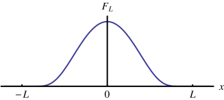
Figure 1: $F_{L}(x)$

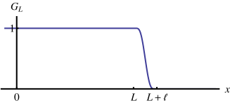
Figure 2: $G_{L}(x)$

The absolute maxima of $F_{L}(x)$ and its derivatives $F_{L}^{(n)}(x)$ are proportional to $L^{-(n+1/2)}$, and the absolute maxima of $G_{L}(x)$ and its derivatives $G_{L}^{(n)}(x)$ are independent of $L$:

$$\max|F_{L}^{(n)}(x)| = \frac{1}{(2L)^{n+1/2}}\max|F^{(n)}(x)|\equiv\frac{1}{L^{n+1/2}}f_{(n)},$$ (B.4)

$$\max|G_{L}^{(n)}(x)| = \frac{1}{\ell^{n}}\max|G^{(n)}(x)|\equiv g_{(n)}.$$ (B.5)

Variables $\lambda^{m_{\mu}}$, $\lambda^{Im_{\mu}}$, $Y_{(\mu)}^{(i_{\mu}j_{\mu})}$ and $Y_{(\mu)}^{I(i_{\mu}j_{\mu})}$ are collectively denoted by $x_{a_{\mu}}$, and let $r_{\mu}$ be

$$r_{\mu} = \sqrt{\sum_{a_{\mu}}(x_{a_{\mu}})^{2}}$$ (B.6)

$$= \sqrt{\sum(\lambda^{m_{\mu}})^{2}+\sum(\lambda^{Im_{\mu}})^{2}+\sum Y_{(\mu)}^{(i_{\mu}j_{\mu})}Y_{(\mu)}^{(j_{\mu}i_{\mu})}+\sum Y_{(\mu)}^{I(i_{\mu}j_{\mu})}Y_{(\mu)}^{I(j_{\mu}i_{\mu})}}$$

$$= \sqrt{\text{tr}(X_{(\mu)}-\Lambda_{(\mu)}I_{(\mu)})^{2}+\text{tr}(X^{I}_{(\mu)}-\Lambda^{I}_{(\mu)}I_{(\mu)})^{2}}.$$

$r_{\mu}$ is invariant under $K$. Take a normalizable energy eigenstate $\psi_{(\mu)}(x_{a_{\mu}})$ of SU($N_{(\mu)}$) subsystem with the eigenvalue $E_{(\mu)}$. It is normalized:

$$||\psi_{(\mu)}||^{2}=\int\prod dx_{a_{\mu}}\psi_{(\mu)}^{\dagger}\psi_{(\mu)}=1,$$ (B.7)

and it is assumed that inner products of derivatives of $\psi_{(\mu)}$ are finite. For instance,

$$\left\langle\psi_{(\mu)},\partial_{x_{a_{\mu}}}\psi_{(\mu)}\right\rangle=\int\prod dx_{a_{\mu}}\psi_{(\mu)}^{\dagger}\partial_{x_{a_{\mu}}}\psi_{(\mu)}$$ (B.8)

is finite. The integral

$$A_{(\mu)L}^{2}=\int\prod dx_{a_{\mu}}(G_{L}(r_{\mu}))^{2}\psi_{(\mu)}^{\dagger}\psi_{(\mu)}$$ (B.9)

is positive, is less than 1, monotonically increases as $L$ increases, and goes to 1 as $L\rightarrow\infty$. $\chi_{(\mu)L}(r_{\mu})$ is defined so that $||\chi_{(\mu)L}\psi_{(\mu)}||=1$:

$$\chi_{(\mu)L}(r_{\mu})\equiv G_{L}(r_{\mu})/A_{(\mu)L}.$$ (B.10)

For $N_{\mu}=1$ we define $\chi_{(\mu)L}$ as $\chi_{(\mu)L}=1$. To show that the diffenrence between $H_{(\mu)}(\chi_{(\mu)L}\psi_{(\mu)})$ and $E_{(\mu)}(\chi_{(\mu)L}\psi_{(\mu)})$ can be made arbitrarily small by taking large $L$, we first show that inner products of $\chi_{(\mu)L}\psi_{(\mu)}$ with some $\chi_{(\mu)L}$ replaced by their derivatives go to zero as $L\rightarrow\infty$. For example,

$$\big{|}\left\langle\chi_{(\mu)L}\psi_{(\mu)},(\partial_{x_{a_{\mu}}}\chi_{(\mu)L})\psi_{(\mu)}\right\rangle\big{|} = A_{(\mu)L}^{-2}\Big{|}\int_{L\leq r_{\mu}\leq L+\ell}\prod dx_{b_{\mu}}G_{L}(r_{\mu})\frac{x_{a_{\mu}}}{r_{\mu}}\partial_{r_{\mu}}G_{L,\ell}(r_{\mu})\psi_{(\mu)}^{\dagger}\psi_{(\mu)}\Big{|}$$ (B.11)

$$< A_{(\mu)L}^{-2}g_{(1)}\int_{L\leq r_{\mu}\leq L+\ell}\prod dx_{b_{\mu}}\psi_{(\mu)}^{\dagger}\psi_{(\mu)}$$

$$\leq A_{(\mu)L}^{-2}g_{(1)}\int_{L\leq r_{\mu}}\prod dx_{b_{\mu}}\psi_{(\mu)}^{\dagger}\psi_{(\mu)}$$

$$= A_{(\mu)L}^{-2}g_{(1)}\Big{(}1-\int_{r_{\mu}\leq L}\prod dx_{b_{\mu}}\psi_{(\mu)}^{\dagger}\psi_{(\mu)}\Big{)}$$

$$\rightarrow 0\quad(L\rightarrow\infty).$$

Similarly, inner products containing second derivatives of $\chi_{(\mu)L}$ can be shown to go to zero as $L\rightarrow\infty$. Then

$$\left\langle\chi_{(\mu)L}\psi_{(\mu)},[H_{(\mu)}-E_{(\mu)}](\chi_{(\mu)L}\psi_{(\mu)})\right\rangle = \left\langle\chi_{(\mu)L}\psi_{(\mu)},\chi_{(\mu)L}[H_{(\mu)}-E_{(\mu)}]\psi_{(\mu)}\right\rangle$$ (B.12)

$$-\left\langle\chi_{(\mu)L}\psi_{(\mu)},\frac{\partial}{\partial x_{a_{\mu}}}\chi_{(\mu)L}\frac{\partial}{\partial x_{a_{\mu}}}\psi_{(\mu)}\right\rangle$$

$$-\frac{1}{2}\left\langle\chi_{(\mu)L}\psi_{(\mu)},\frac{\partial^{2}}{\partial x_{a_{\mu}}^{2}}\chi_{(\mu)L}\psi_{(\mu)}\right\rangle$$

$$\rightarrow 0\quad(L\rightarrow\infty).$$

Similarly, $\left\langle[H_{(\mu)}-E_{(\mu)}](\chi_{(\mu)L}\psi_{(\mu)}),[H_{(\mu)}-E_{(\mu)}](\chi_{(\mu)L}\psi_{(\mu)})\right\rangle\rightarrow 0\quad(L\rightarrow\infty)$.

Next we define (the bosonic part of) $\chi_{L,E}$. $Q_{MN}=h_{(0)M}^{\mu}{\cal N}_{\mu\nu}h_{(0)N}^{\nu}$ is real and symmetric, and therefore is diagonalizable by an orthogonal matrix $W_{MN}$: $Q_{MN}=q_{L}W_{ML}W_{NL}$. The eigenvalues $q_{M}$ are real. Noting that $Q_{MN}$ satisfies $(Q^{n})_{MN}=h_{(0)M}^{\mu}({\cal N}^{n})_{\mu\nu}h_{(0)N}^{\nu}$, its eigenvalue equation $0=\det(Q-qI)\equiv w(q)$ is evaluated as

$$w(q)=-\frac{1}{N}\left(\sum_{\mu}\frac{N_{\mu}}{N_{\mu}-q}\right)\prod_{\nu}(N_{\nu}-q).$$ (B.13)

Since $w(q)<0$ for $q\leq 0$, all the eigenvalues $q_{M}$ are positive.

Let $\Lambda^{a}$ denote $\Lambda^{N}W_{NM}$ and $\Lambda^{IN}W_{NM}$. Then $H_{1}=-\frac{1}{2}q_{a}\frac{\partial}{\partial\Lambda^{a}}\frac{\partial}{\partial\Lambda^{a}}$, and $\chi_{L,E}$ is defined as

$$\chi_{L,E}(\Lambda^{a})\equiv\prod_{b}F_{L}(\Lambda^{b})e^{ik_{b}\Lambda^{b}},$$ (B.14)

where $k_{a}$ are arbitrary real numbers satisfying $\sum_{a}q_{a}k_{a}k_{a}=2E$. $q_{a}$ is defined as $q_{M}$ for $a=M$ and $a=IM$. $\chi_{L,E}$ is normalized:

$$||\chi_{L,E}||^{2}=\int_{-\infty}^{\infty}\prod_{a}d\Lambda^{a}|\chi_{L,E}(\Lambda^{a})|^{2}=1.$$ (B.15)

Note that $\prod_{M}d\Lambda^{M}\prod_{I,N}d\Lambda^{IN}=\prod_{a}d\Lambda^{a}$. We can show that the difference between $H_{1}\chi_{L,E}$ and $E\chi_{L,E}$ can be made arbitrarily small by taking large $L$. For example,

$$\big{|}\left\langle\chi_{L,E},[H_{1}-E]\chi_{L,E}\right\rangle\big{|} = \frac{1}{2}\left|\int_{-\infty}^{\infty}\prod_{a}d\Lambda^{a}\chi_{L,E}^{\dagger}q_{b}\left(-\frac{d}{d\Lambda^{b}}\frac{d}{d\Lambda^{b}}-k_{b}k_{b}\right)\chi_{L,E}\right|$$ (B.16)

$$= \frac{1}{2}\left|\int_{-L}^{L}dxF_{L}(x)\left(-\sum_{a}q_{a}\frac{d^{2}}{dx^{2}}-2iq_{b}k_{b}\frac{d}{dx}\right)F_{L}(x)\right|$$

$$< \frac{1}{2}\int_{-L}^{L}dx\frac{f_{(0)}}{L^{1/2}}\left(\Big{|}\sum_{a}q_{a}\Big{|}\frac{f_{(2)}}{L^{5/2}}+2|q_{a}k_{a}|\frac{f_{(1)}}{L^{3/2}}\right)$$

$$< f_{(0)}\left(\Big{|}\sum_{a}q_{a}\Big{|}\frac{f_{(2)}}{L^{2}}+2|q_{a}k_{a}|\frac{f_{(1)}}{L}\right)$$

$$\rightarrow 0\quad(L\rightarrow\infty).$$

Similarly, $\left\langle[H_{1}-E]\chi_{L,E},[H_{1}-E]\chi_{L,E}\right\rangle\rightarrow 0\quad(L\rightarrow\infty)$.

Appendix C Smoothness of eigenvalues and unitary transformations

Eigenvalues of matrices are determined by solving the eigenvalue equations. Let us consider an $N\times N$ matrix $A=(a_{ij})$, and let its eigenvalues be $y_{i}$. Then the eigenvalue equation

$$0=F(y,\bm{x})\equiv y^{N}+x_{1}y^{N-1}+x_{2}y^{N-2}+\dots+x_{N}=(y-y_{1}(\bm{x}))(y-y_{2}(\bm{x}))\dots(y-y_{N}(\bm{x}))$$ (C.1)

is an algebraic equation of degree $N$, and its coefficients $x_{i}$, or $\bm{x}$ collectively, are smooth functions of $a_{ij}$. Since, in general, solutions to algebraic equations are continuous functions of coefficients of the equations, $y_{i}=y_{i}(\bm{x})$ are continuous functions of $\bm{x}$, or $a_{ij}$. However $y_{i}=y_{i}(\bm{x})$ are not always differentiable, as can be easily seen from explicit expressions of solutions to equations of lower degrees. By applying the standard implicit function theorem to (C.1), we see that if $y_{i}(\bm{x}_{0})$ is not equal to $y_{j}(\bm{x}_{0})$ for any $j\not\neq i$, $y_{i}(\bm{x})$ is smooth in the neighborhood of $\bm{x}_{0}$. When the equation has multiple solutions $y_{i}(\bm{x}_{0})=y_{j}(\bm{x}_{0})$, the implicit function theorem cannot be applied at $\bm{x}=\bm{x}_{0}$ because of $\partial_{y}F(y_{i}(\bm{x}_{0}),\bm{x}_{0})=0$.

Even when we have multiple solutions, we can show that the sum of those solutions are smooth: If $y_{1}(\bm{x}_{0})=y_{2}(\bm{x}_{0})=\dots=y_{n}(\bm{x}_{0})$ and $y_{1}(\bm{x}_{0})\not\neq y_{i}(\bm{x}_{0})$ for $i\geq n$, $y_{1}(\bm{x})+y_{2}(\bm{x})+\dots+y_{n}(\bm{x})$ is smooth at $\bm{x}_{0}$. In addition, $[y_{1}(\bm{x})]^{q}+[y_{2}(\bm{x})]^{q}+\dots+[y_{n}(\bm{x})]^{q}$ are also smooth for any positive integer $q$. This can be shown as follows: We regard the function $F(y,\bm{x})$ as one on the complex plane $y\in\mathbb{C}$, then the following holds in the neighborhood of $\bm{x}_{0}$.

$$[y_{1}(\bm{x})]^{q}+[y_{2}(\bm{x})]^{q}+\dots+[y_{n}(\bm{x})]^{q}=\oint_{C(\bm{x}_{0})}\frac{dy}{2\pi i}\frac{y^{q}\partial_{y}F(y,\bm{x})}{F(y,\bm{x})},$$ (C.2)

where the fixed contour $C(\bm{x}_{0})$ encircles $y=y_{1}(\bm{x}_{0}),y_{2}(\bm{x}_{0}),\dots$ and $y_{n}(\bm{x}_{0})$. From the continuity of $y_{i}(\bm{x})$, $y=y_{1}(\bm{x}),y_{2}(\bm{x}),\dots$ and $y_{n}(\bm{x})$ are on the inside of $C(\bm{x}_{0})$, and $y=y_{n+1}(\bm{x}),y_{n+2}(\bm{x}),\dots$ and $y_{N}(\bm{x})$ are on the outside of $C(\bm{x}_{0})$ for any $\bm{x}$ near $\bm{x}_{0}$. Clearly the right hand side of (C.2) is differentiable at $\bm{x}_{0}$ with respect to $\bm{x}$.

If $A=(a_{ij})$ is hermitian, it is diagonalizable by a unitary matrix $u$: $uAu^{-1}=\text{diag}(y_{1},y_{2},\dots,y_{N})$, and eigenvalues $y_{i}$ are real. Although $y_{i}$ are continuous functions of $a_{ij}$, elements of $u$ are not even continuous at the points where some of the eigenvalues degenerate. Let us see this in detail. $u$ is constructed from normalized eigenvectors $\bm{v}_{i}$ as follows:

$$u^{\dagger}=(\bm{v}_{1},\bm{v}_{2},\dots,\bm{v}_{N}),\quad A\bm{v}_{i}=y_{i}\bm{v}_{i},\quad\bm{v}^{\dagger}_{i}\cdot\bm{v}_{i}=1,$$ (C.3)

and when $y_{i}$ is not a degenerate eigenvalue,

$$\bm{v}_{i}\propto\begin{pmatrix}\widetilde{\Delta}^{(i)}_{j1}\\ \widetilde{\Delta}^{(i)}_{j2}\\ \vdots\\ \widetilde{\Delta}^{(i)}_{jN}\end{pmatrix},\quad\widetilde{\Delta}^{(i)}_{kl}=(k,l)~{}\text{cofactor of}~{}A-y_{i}I,$$ (C.4)

for any $j$. Since the rank of $A-y_{i}I$ is $N-1$, at least one of $\widetilde{\Delta}^{(i)}_{kl}$ is nonzero. So we can choose $j$ such that $\bm{v}_{i}$ is a nonzero vector. Then $\bm{v}_{i}$ is given by

$$\bm{v}_{i}=\frac{1}{\sqrt{\sum_{k}|\widetilde{\Delta}^{(i)}_{jk}|^{2}}}\begin{pmatrix}\widetilde{\Delta}^{(i)}_{j1}\\ \widetilde{\Delta}^{(i)}_{j2}\\ \vdots\\ \widetilde{\Delta}^{(i)}_{jN}\end{pmatrix}.$$ (C.5)

Since $\widetilde{\Delta}^{(i)}_{kl}$ are smooth functions of $a_{ij}$, so is $\bm{v}_{i}$. However, when $y_{i}$ becomes degenerate, all of $\widetilde{\Delta}^{(i)}_{kl}$ vanish, and the above expression of $\bm{v}_{i}$ is not well-defined. (We can take a limit into the point where $y_{i}$ is degenerate, but the limit depends on how we approach the point.)

If we consider $A$ only in a region $R$, where $R$ is such that $A$ always has a degenerate eigenvalue throughout the region, we can find smooth orthonormal eigenvectors. ($R$ usually has nonzero codimension in the entire space of $a_{ij}$.) Let $A$ have $r$-fold eigenvalue $0$ in $R$, and let other eigenvalues never be zero in $R$. Then the rank of $A$ is $N-r$, and there exists nonzero $(N-r)\times(N-r)$ cofactor. if

$$\Delta\equiv\det\begin{pmatrix}a_{11}&a_{12}&\dots&a_{1,N-r}\\ a_{21}&a_{22}&\dots&a_{2,N-r}\\ \vdots&&\ddots&\vdots\\ a_{N-r,1}&a_{N-r,2}&\dots&a_{N-r,N-r}\end{pmatrix}$$ (C.6)

is nonzero, then $r$ eigenvectors $\bm{v}_{1},\dots,\bm{v}_{r}$ corresponding to the eigenvalue $0$ are

$$\bm{v}_{1}\propto\begin{pmatrix}\Delta_{11}\\ \Delta_{21}\\ \vdots\\ \Delta_{N-r,1}\\ -\Delta\\ 0\\ 0\\ \vdots\\ 0\end{pmatrix},\quad\bm{v}_{2}\propto\begin{pmatrix}\Delta_{12}\\ \Delta_{22}\\ \vdots\\ \Delta_{N-r,2}\\ 0\\ -\Delta\\ 0\\ \vdots\\ 0\end{pmatrix},\quad\dots,\quad\bm{v}_{r}\propto\begin{pmatrix}\Delta_{1r}\\ \Delta_{2r}\\ \vdots\\ \Delta_{N-r,r}\\ 0\\ 0\\ \vdots\\ 0\\ -\Delta\end{pmatrix},$$ (C.7)

where $\Delta_{ij}$ is $\Delta$ with $i$-th column replaced by $(a_{1,N-r+j},a_{2,N-r+j},\dots,a_{N-r,N-r+j})^{T}$. $\Delta_{ij}$ and $\Delta$ are smooth functions of $a_{ij}$, and $\bm{v}_{i}$ can be smoothly orthonormalized by Gram-Schmidt process where $\Delta$ is nonzero. If $\Delta=0$, we can replace $\Delta$ by other nonzero $(N-r)\times(N-r)$ cofactors and can construct $r$ smooth eigenvectors similarly to the above. When two $(N-r)\times(N-r)$ cofactors are nonzero, we can construct two sets of $r$ smooth orthonormal eigenvectors $\{\bm{e}_{1},\dots,\bm{e}_{r}\}$ and $\{\bm{f}_{1},\dots,\bm{f}_{r}\}$, and these vectors are related to each other by the smooth unitary matrix $V_{ji}=\bm{f}_{j}^{\dagger}\cdot\bm{e}_{i}$: $\bm{e}_{i}=\bm{f}_{j}V_{ji}$. Therefore, if $A$ goes out of the region where $\Delta\not\neq 0$ into another region where another $(N-r)\times(N-r)$ cofactor is nonzero as we change the elements of $A$ continuously, we can use the ”transition matrix” $V_{ji}$ to keep the smoothness of the eigenvectors. (This is similar to the situation we encounter when we go from one coordinate patch to another on a manifold.)

Using the above fact, we can show that if two sets of eigenvalues $\{y_{1},y_{2},\dots,y_{r}\}$ and $\{y_{r+1},y_{r+2},\dots,y_{N}\}$ have no intersection, then there exist a smooth unitary matrix $U$, a smooth hermitian $r\times r$ matrix $A_{1}$, and a smooth hermitian $(N-r)\times(N-r)$ matrix $A_{2}$ such that

$$UAU^{-1}=\begin{pmatrix}A_{1}&0\\ 0&A_{2}\end{pmatrix},$$ (C.8)

and, $A_{1}$ and $A_{2}$ have eigenvalues $\{y_{1},y_{2},\dots,y_{r}\}$ and $\{y_{r+1},y_{r+2},\dots,y_{N}\}$ respectively.

This can be shown by using the following hermitian matrix:

$${\cal A}\equiv(A-y_{1}I)(A-y_{2}I)\dots(A-y_{r}I)=\sum_{n=0}^{r}(-1)^{n}P_{n}A^{r-n},$$ (C.9)

where $P_{0}=1$ and $P_{m}=\sum_{1\leq i_{1}<i_{2}<\dots<i_{m}\leq r}y_{i_{1}}y_{i_{2}}\dots y_{i_{m}}$. $P_{m}$ can be expressed in terms of $\sum_{i=1}^{r}(y_{i})^{q}$, which we have already shown to be smooth. Therefore elements of ${\cal A}$ are also smooth. ${\cal A}$ has $r$-fold degenerate eigenvalue $0$, and we have already shown that we can construct $r$ smooth orthonormal eigenvectors $\bm{e}_{1},\bm{e}_{2},\dots,\bm{e}_{r}$ which span the union of the eigenspaces of $A$ corresponding to eigenvalues $\{y_{1},y_{2},\dots,y_{r}\}$. Similarly, by considering ${\cal A}^{\prime}\equiv(A-y_{r+1}I)(A-y_{r+2}I)\dots(A-y_{N}I)$, we can construct smooth orthonormal vectors $\bm{e}^{\prime}_{1},\bm{e}^{\prime}_{2},\dots,\bm{e}^{\prime}_{N-r}$ which span the union of the eigenspaces of $A$ corresponding to eigenvalues $\{y_{r+1},y_{r+2},\dots,y_{N}\}$. These two sets of vectors are orthogonal to each other. Therefore

$$U^{\dagger}=(\bm{e}_{1},\bm{e}_{2},\dots,\bm{e}_{r},\bm{e}^{\prime}_{1},\bm{e}^{\prime}_{2},\dots,\bm{e}^{\prime}_{N-r})$$ (C.10)

is unitary and smooth, and satisfies (C.8). When we have to go out of the region where $\bm{e}_{i}$ and $\bm{e}^{\prime}_{i}$ are well-defined, we can use the ”transition matrix” of the block diagonal form to keep the smoothness of $U$, $A_{1}$ and $A_{2}$:

$$U^{\dagger}\rightarrow U^{\dagger}\begin{pmatrix}V_{1}^{\dagger}&0\\ 0&V_{2}^{\dagger}\end{pmatrix}$$ (C.11)

i.e. if we parametrize the space of $a_{ij}$ by $A_{1}$, $A_{2}$ and $U$, we need some coordinate patches, and those patches are connected by the transition matrices.

By applying this fact repeatedly, $A$ can be block diagonalized into smaller hermitian matrices $A_{i}$ by a smooth unitary matrix, corresponding to disjoint sets of eigenvalues:

$$UAU^{-1}=A_{D}\equiv\begin{pmatrix}A_{1}&&&\\ &A_{2}&&\\ &&\ddots&\\ &&&A_{n}\end{pmatrix}.$$ (C.12)

Each $A_{i}$ can further be diagonalized by multiplying appropriate block diagonal unitary matrix $u$ to (C.12):

$$uUAU^{-1}u^{-1}=\begin{pmatrix}y_{1}&&&\\ &y_{2}&&\\ &&\ddots&\\ &&&y_{N}\end{pmatrix},\quad u=\begin{pmatrix}U_{1}&&&\\ &U_{2}&&\\ &&\ddots&\\ &&&U_{n}\end{pmatrix},$$ (C.13)

but these $U_{i}$ are not necessarily smooth.

If we have a smooth function $\hat{f}(A_{D})$ of $A_{D}$ which is invariant under the action of block diagonal unitary matrices $u$: $\hat{f}(A_{D})=\hat{f}(uA_{D}u^{-1})$, then it can be extended to a smooth function $f(A)=\hat{f}(A_{D})$ of $A=U^{-1}A_{D}U$ which is invariant under the action of unitary matrices: $f(A)=f(U^{\prime}AU^{\prime-1})$. Note that due to the invariance $\hat{f}(A_{D})=\hat{f}(uA_{D}u^{-1})$, the transition matrix (C.11) can act on $A_{D}$ consistently.

References

[1]
B. de Wit, J. Hoppe and H. Nicolai,
“On the quantum mechanics of supermembranes”,
Nucl. Phys.B305 (1988) 545.
[2]
T. Banks, W. Fischler, S. Shenker and L. Susskind,
“M Theory As A Matrix Model: A Conjecture”,
Phys. Rev.D55 (1997) 6189, hep-th/9610043.
[3]
L. Susskind,
“Another Conjecture about M(atrix) Theory”,
hep-th/9704080.
[4]
B. de Wit, M. Luscher and H. Nicolai,
“The Supermembrane Is Unstable”,
Nucl. Phys.B320 (1989) 135.
[5]
A. V. Smilga,
“Comments on thermodynamics of supersymmetric matrix models”,
Nucl. Phys.B818 (2009) 101,
arXiv:0812.4753 [hep-th].
[6]
J. Plefka and A. Waldron,
“On the quantum mechanics of M(atrix) theory”,
Nucl. Phys.B512 (1998) 460,
hep-th/9710104