Network-based multivariate gene-set testing

Abstract

The identification of predefined groups of genes (“gene-sets”) which are differentially expressed between two conditions (“gene-set analysis”, or GSA) is a very popular analysis in bioinformatics. GSA incorporates biological knowledge by aggregating over genes that are believed to be functionally related. This can enhance statistical power over analyses that consider only one gene at a time. However, currently available GSA approaches are all based on univariate two-sample comparison of single genes. This means that they cannot test for differences in covariance structure between the two conditions. Yet interplay between genes is a central aspect of biological investigation and it is likely that such interplay may differ between conditions. This paper proposes a novel approach for gene-set analysis that allows for truly multivariate hypotheses, in particular differences in gene-gene networks between conditions. Testing hypotheses concerning networks is challenging due the nature of the underlying estimation problem. Our starting point is a recent, general approach for high-dimensional two-sample testing. We refine the approach and show how it can be used to perform multivariate, network-based gene-set testing. We validate the approach in simulated examples and show results using high-throughput data from several studies in cancer biology.

Keywords Gene-set testing, Gaussian graphical models, Differential network, Graphical Lasso, Cancer biology

1 Introduction

Differential expression analysis (Tusher et al., 2001; Lönnstedt and Speed, 2002; Smyth, 2004) is one of the most popular statistical analyses in molecular biology, whether for mRNA (including RNA-seq and microarrays), protein or epigenomic data. For each variable (or gene, we use both terms interchangeably throughout but note that methods described apply also to other types of data) expression levels are compared between conditions of interest to obtain a measure of significance for the gene, usually accounting for multiple comparisons.

Subramanian et al. (2005) pointed out a number of drawbacks of classical, single gene differential expression analysis, including lack of statistical power and difficulties in interpreting significant genes in a biological context. They addressed these concerns by an approach called gene-set analysis or GSA which sought to test differential expression not at the level of single genes in isolation, but rather using (pre-defined) groups of biologically related genes called gene-sets. GSA can provide gains in power by taking advantage of the biological knowledge encoded in gene-set membership: for example, if several members of a certain gene-set all show a moderate change between conditions, the gene-set as whole may be significant even if its constituent genes would not be significant on a gene-by-gene basis. Furthermore, by providing results at the level of biologically meaningful sets of genes, GSA can aid in interpretation of the results of differential expression analysis. GSA has become one of the most widely used analyses in bioinformatics. Irizarry et al. (2009) provide a self-contained introduction to GSA aimed at a statistical audience; GSA and extensions thereof are further described in Subramanian et al. (2005); Efron and Tibshirani (2007); Jiang and Gentleman (2007).

GSA focuses on multiple genes taken together. However, existing GSA approaches (Subramanian et al., 2005; Irizarry et al., 2009; Efron and Tibshirani, 2007) are based on univariate statistics comparing the two conditions of interest. That is, they aggregate several single-gene comparisons to arrive at a gene-set-level statistic and measure of significance. In these procedures, for each gene $j=1,\ldots,p$ a two-sample statistic $z_{j}$ is computed. The $z_{j}$’s for genes belonging to specific gene-sets $A_{s},s=1,\ldots,S$ are then combined to arrive at aggregate scores $a_{s}$ at the gene-set-level. Despite the usefulness of these approaches they have a major limitation in that they are all based on single-gene comparisons and are therefore inherently univariate in nature. In particular, changes in covariance structure between two conditions cannot be tested by such approaches. However, interplay between molecular variables is a fundamental aspect of biology and it is likely that in many settings differences in covariance or conditional independence structure between conditions may be relevant. These observations motivate a need to extend classical GSA in a multivariate direction.

This article is about extending GSA to allow assessment of the importance or significance of gene-sets via multivariate statistics. As we describe below, the approach we propose can be interpreted as testing for differences between conditions at the level of networks. To describe gene-gene networks we use graphical models in which the absence/presence of edges corresponds to conditional independence statements. The method we propose for multivariate, network-based gene-set testing is called NetGSA. For each gene-set, NetGSA carries out a multivariate, network-based comparison between conditions (details are outlined below), adjusts the obtained p-values for multiple comparison and finally provides a list of gene-sets ordered by significance. The results of NetGSA (focusing on differences at the network level) can also be combined with those obtained from “classical” GSA to determine significance in terms of both networks and change in average gene expression.

Network-based gene-set analysis is challenging. It requires two-sample comparison between networks for typically hundreds of gene-sets and involves issues of high-dimensionality and multiplicity. The intention is not to compare two known networks, but rather to test significance of differences between two estimated networks. High-dimensionality poses severe challenges in this setting since the number of samples is typically small compared to the large parameter spaces required for describing the networks. This makes estimation of graphical model structure (“network inference”) a challenging problem, and the difficulties are inherited in the case of two-sample comparison of estimated networks.

The proposed approach for gene-set testing is based on recently developed methodology for high-dimensional two-sample testing described in Städler and Mukherjee (2013) and in particular on an approach called differential network or DiffNet which quantifies the difference between two networks inferred from different populations by a p-value. DiffNet is based on the sample splitting technique introduced by Wasserman and Roeder (2009): the data is randomly split into two halves, networks are inferred on one half and significance testing (p-value calculation) is performed on the other half. This process is repeated many times in order to prevent a “p-value lottery” due to the arbitrary choice of the data split (Meinshausen et al., 2009).

To the best of our knowledge, DiffNet is currently the only available approach that allows two-sample testing in high-dimensional graphical models. Note, that permutation-based tests are computationally not feasible here as a large number of permutations would be necessary to compensate the multiple testing correction. We restrict attention to multivariate comparisons at the gene-set level; that is, we test networks whose nodes are identified with members of gene-sets, and whose edges are within rather than between gene-sets. The general approach of Städler and Mukherjee (2013) could in principle be applied to comparison of full, $p$-dimensional distributions or networks between conditions, but this is a very difficult high-dimensional problem and is beyond the scope of this paper.

The approach we propose can in principle be used with any graphical model formulation. However, for NetGSA network analyses have to be conducted for each gene-set. There are typically hundreds of gene-sets and the number genes per gene-set can vary from a few up to several dozens of genes. Thus, network inference (NI) approaches used in DiffNet have to be computationally efficient, and chosen and tuned carefully. They need to be able to deal automatically with different numbers of nodes (genes), they have to satisfy two conditions related to potential overfitting (screening and sparsity assumptions). We focus on Gaussian graphical models (GGMs) and compare a number of specific approaches for their estimation. The overall procedure we propose is computationally efficient and naively parallelizable: for analysis of a lung cancer gene expression dataset reported below, with $d=1208$ genes and $S=216$ gene-sets, computation required $52$ minutes on a multicore system using $50$ cores (each $1.5$ GHz) and $504$ GB shared memory.

Section 2 introduces our main methodology for network-based gene-set testing: Section 2.1 formulates the hypothesis testing problem; Section 2.2 expands on DiffNet (Städler and Mukherjee, 2013); Section 2.3 describes our novel algorithm NetGSA; Section 2.4 discusses different network inference (NI) approaches. In Section 3 we report on simulation results and real data examples from cancer biology are investigated in Section 4.

2 Methods

2.1 Notation and set-up

Let $\mathbf{X}$ and $\mathbf{Y}$ be matrices of gene expression levels obtained under two conditions. The dimension of $\mathbf{X}$, $\mathbf{Y}$ are $n_{x}\times d$ and $n_{y}\times d$ respectively, where $d$ denotes the total number of genes under study and $n_{x}$ and $n_{y}$ are the condition-specific sample sizes (throughout we use $x$ and $y$ to denote the two conditions). Gene-sets are denoted $A_{s}\subset\{1,\ldots,d\}$, $s=1,\ldots,S$; gene-sets need not be disjoint. We denote the probability density function of genes belonging to set $A_{s}$ by $f^{x}_{s}$ and $f^{y}_{s}$ for conditions $x$ and $y$ respectively; these densities are joint over all genes belonging to the gene-set and accordingly have dimension $d_{s}$, where $d_{s}=|A_{s}|$.

For a specific gene-set $A_{s}$, our aim is to test whether or not the two conditions have different graphical model or network structure. We use Gaussian graphical models (GGM) to model condition-specific conditional independence structure. Vertices in the graphical models for gene-set $A_{s}$ are identified with members of the gene-set and edges with conditional independence statements between them. We first present NetGSA focusing on testing network differences only and do not test also for differences in the mean; we therefore assume the Gaussian distributions $f^{x}_{s}$ and $f^{y}_{s}$ have identical, zero mean but potentially non-identical concentration matrices denoted by $\Omega^{x}_{s}$ and $\Omega^{y}_{s}$ respectively. The edge structure or network of the corresponding graphical models are defined by

$$(\Omega^{x}_{s})_{j,j^{\prime}}=0\Leftrightarrow(j,j^{\prime})\notin E(G^{x}_{s})\quad\textrm{and}\quad(\Omega^{y}_{s})_{j,j^{\prime}}=0\Leftrightarrow(j,j^{\prime})\notin E(G^{y}_{s})$$

where $G^{x}_{s}$ and $G^{y}_{s}$ are undirected graphs associated with the condition-specific graphical models and $E(G)$ denotes the edge set of graph $G$.

Thus, for gene-set $A_{s}$, the NetGSA null hypothesis is

$$\mathbf{H}_{0,s}:\;\Omega^{x}_{s}=\Omega^{y}_{s}.$$ (2.1)

To test these hypotheses, our strategy is to use Differential Network (described in Section 2.2) to test each gene-set separately and then correct the obtained p-values for multiple testing. Note that gene-sets contain different numbers of genes which can vary from moderate to very large. As the sample sizes $n_{x}$ and $n_{y}$ are typically small, testing (2.1) is challenging and involves issues of high-dimensionality.

2.2 Differential networks

We recently developed a novel and very general approach for high-dimensional two-sample testing (Städler and Mukherjee, 2013). We also outlined how to use the approach for two-sample comparison of graphical models (differential network or DiffNet). In this Section we review DiffNet with reference to the NetGSA context; we refer the reader to Städler and Mukherjee (2013) for further technical details.

2.2.1 Network testing using sample splitting

Consider a gene-set $A_{s}$ and corresponding gene expression matrices $\mathbf{X}_{s}$ and $\mathbf{Y}_{s}$ for the two conditions (of size $n_{x}\times d_{s}$ and $n_{y}\times d_{s}$ respectively). For each condition, we randomly split the data into two halves $\mathbf{X}_{s}=(\mathbf{X}^{\rm in}_{s},\mathbf{X}^{\rm out}_{s})$ and $\mathbf{Y}_{s}=(\mathbf{Y}^{\rm in}_{s},\mathbf{Y}^{\rm out}_{s})$. To test the hypothesis $\mathbf{H}_{0,s}:\Omega^{x}_{s}=\Omega^{y}_{s}$, DiffNet proceed in two steps:

1. Network screening step. Based on the first half of the data, $\mathbf{X}^{\rm in}_{s}$ and $\mathbf{Y}^{\rm in}_{s}$, networks $\hat{G}^{x}_{s}$ and $\hat{G}^{y}_{s}$ are estimated for each condition separately. In addition, a third network $\hat{G}^{xy}_{s}$ is built using pooled data ($\mathbf{X}^{\rm in}_{s}$,$\mathbf{Y}^{\rm in}_{s}$). The latter network should provide a good model in the null case of no difference between the two conditions. Under the alternative, however, modeling both conditions with different graphs $\hat{G}^{x}_{s}$ and $\hat{G}^{y}_{s}$ is beneficial. We propose and compare several ways of inferring the networks $\hat{G}^{x}_{s}$, $\hat{G}^{y}_{s}$ and $\hat{G}^{xy}_{s}$ in Section 2.4.

2. P-value calculation step. The networks $\hat{G}^{x}_{s}$ and $\hat{G}^{y}_{s}$ model each condition individually and give rise to a log-likelihood $L^{\rm ind}_{s}=L_{\hat{G}^{x}_{s}}+L_{\hat{G}^{y}_{s}}$. On the other hand, $\hat{G}^{xy}_{s}$ models pooled data jointly with log-likelihood $L^{\rm joint}_{s}=L_{\hat{G}^{xy}_{s}}$. We compare the individual with the joint model using the score

   $${\Delta}\mathrm{AIC}_{s} = \mathrm{AIC}^{\rm ind}_{s}-\mathrm{AIC}^{\rm joint}_{s}$$

   $$= 2\left(L^{\rm ind}_{s}-L^{\rm joint}_{s}\right)-2(\mathrm{df}^{\rm ind}_{s}-\mathrm{df}^{\rm joint}_{s}),$$

   with degrees of freedom $\mathrm{df}^{\rm ind}_{s}=2d_{s}+|E(\hat{G}^{x}_{s})|+|E(\hat{G}^{y}_{s})|$ and $\mathrm{df}^{\rm joint}_{s}=d_{s}+|E(\hat{G}^{xy}_{s})|$. This score is based on the Akaike Information Criterion (AIC). We emphasize that all log-likelihoods appearing in ${\Delta}\mathrm{AIC}_{s}$ are evaluated using the second half of the data and involve maximum likelihood estimation with constraints given by the graphs. If $\mathbf{X}$ and $\mathbf{Y}$ arise from different networks, then we expect ${\Delta}\mathrm{AIC}_{s}$ to be larger than zero. In fact, it can be shown that ${\Delta}\mathrm{AIC}_{s}$ tends to infinity for large sample sizes. On the other hand, under the null hypothesis, ${\Delta}\mathrm{AIC}_{s}$ is asymptotically distributed as a shifted weighted-sum-of-chi-quares with distribution function $\Psi(\cdot;\nu,\delta)$, weights $\nu=(\nu_{1},\ldots,\nu_{r})$ and shift $\delta=2(\mathrm{df}^{\rm ind}_{s}-\mathrm{df}^{\rm joint}_{s})$. As a consequence a p-value for the hypothesis $H_{0,s}$ can be obtained by

   $$\mathrm{p}^{s} = 1-\Psi(\Delta\mathrm{AIC}_{s};\nu,\delta).$$ (2.3)

   For all details, in particular on the computation of the weights $\nu$, we refer to Städler and Mukherjee (2013).

2.2.2 Screening and sparsity assumptions

There are two key assumptions in the above procedure which are mandatory to obtain correct p-values which control the type-I error. Both involve the network inference approach used in the first step of DiffNet. Consider a $n\times d$ data matrix $\mathbf{X}$ generated from a GGM with graph $G$. Then, the estimated graph $\hat{G}(\mathbf{X})$ has to satisfy:

• Screening assumption (ScA). The edge set of the inferred graph contains the edge set of the true data generating graph: $E(G)\subseteq E(\hat{G}).$

• Sparsity assumption (SpA). The inferred networks are sparse, i.e., the number of edges $|E(\hat{G})|$ is not too large compared to the sample size $n$.

Both assumptions are important. ScA guarantees that the models involved in the test statistic are correctly specified and that $\Delta\mathrm{AIC}_{s}$ has asymptotic null-distribution $\Psi(\cdot;\nu,\delta)$. SpA is necessary to ensure maximum likelihood estimation in the second split is well-behaved and to render the asymptotic approximation of the null-distribution accurate.

2.2.3 Sparsity index

To monitor sparsity we use a sparsity index $m(\hat{G})$ defined as:

$$m(\hat{G}) = \frac{2|E(\hat{G})|}{n\times p}.$$ (2.4)

This quantity has a motivation in terms of linear regression: estimating the concentration matrix of a GGM with graph $G$ can be done by regressing each variable (or node) $j$ against all neighbouring variables $\mathrm{nb}_{j}=\{i:(i,j)\in E(G)\}\subset\{1,\ldots,k\}$. If we assume that neighbouring sets are of approximately the same size ($|\mathrm{nb}_{j}|\approx\mathrm{const}$) then the inverse $1/m(G)$ of the sparsity index for graph $G$ can be interpreted as the number of samples per predictor. In linear regression a typical rule of thumb is $5$ to $10$ samples per predictor to obtain well-behaved parameter estimation. Later, we use the sparsity index $m$ to carry out adaptive thresholding to ensure estimation and p-value calculation in the second split are well-behaved.

In Section 2.4 we discuss different GGM estimation procedures from the literature and discuss their properties in terms of the screening and sparsity assumptions.

2.3 The NetGSA algorithm

By applying DiffNet to all gene-sets $A_{s}$, $s=1,\ldots,S$ we get p-values $p^{s}$, $s=1,\ldots,S$. To test (2.1) we then adjust these values for multiple comparison and obtain the corrected p-values $\tilde{\mathrm{p}}^{s}$, $s=1,\ldots,S$. The outcome depends heavily on the initial data splitting (see Section 2.2). Depending on the random split of the data we can get different results which amounts to a “p-value lottery” (Meinshausen et al., 2009). To get stable and reproducible results we therefore repeat the splitting process many times and aggregate the resulting p-values. A simple approach combines the p-values by taking the median (van de Wiel et al., 2009). Algorithm 1 summarizes the overall procedure which we call NetGSA.

Input Data $\mathbf{X}$ and $\mathbf{Y}$, gene-sets $A_{s}$, $s=1,\ldots,S$, number of data splits $B$.

1:Randomly split data into two halves

2:for $s=1,\ldots,S$ do

3:     Network Screening (on 1st half) Using a network inference procedure, infer networks $\hat{G}^{x}_{s}$, $\hat{G}^{y}_{s}$ and $\hat{G}^{xy}_{s}$.

4:     P-values (on 2nd half) Evaluate $L^{\rm ind}_{s}=L_{\hat{G}^{x}_{s}}+L_{\hat{G}^{y}_{s}}$, $L^{\rm joint}_{s}=L_{\hat{G}^{xy}_{s}}$ and $\mathrm{df}^{\rm ind}_{s}$, $\mathrm{df}^{\rm joint}_{s}$. Evaluate $\Delta\mathrm{AIC}_{s}=\mathrm{AIC}^{\rm ind}_{s}-\mathrm{AIC}^{\rm joint}_{s}.$ Obtain $\mathrm{p}^{s}=1-\Psi(\Delta\mathrm{AIC}_{s};\nu,\delta)$, where $\delta=2(\mathrm{df}^{\rm ind}_{s}-\mathrm{df}^{\rm joint}_{s})$ and $\nu$ are weights estimated following Städler and Mukherjee (2013).

5:end for

6:Calculate FDR-corrected p-values: $\tilde{\mathrm{p}}^{1},\ldots,\tilde{\mathrm{p}}^{S}$.

7:Repeat steps 1-6 $B$ times.

Output Aggregated quantities (median over $B$ splits): $\tilde{\mathrm{p}}^{s,\rm med}$ ($s=1,\ldots,S$).

Algorithm 1 NetGSA: Network-based gene-set analysis

We point out that Algorithm 1 tests only for differences in terms of networks and does not pick-up changes between the two conditions due to a difference in mean level. We propose below a simple procedure for combining the results of NetGSA as described above with standard approaches for mean-based GSA to obtain a combined gene-set test that captures differences in networks and the mean.

2.4 Network Inference (NI) Approaches

Network inference (NI) is an important part of DiffNet. In Section 2.2 we pointed out that NI has to be in line with ScA and SpA in order to obtain valid p-values. Besides that, NI is the limiting factor in the overall computational complexity of Algorithm 1. Note that three networks have to be inferred for each of the $S$ gene-sets in each of the $B$ data splits. Thus, in total there are $3\times S\times B$ networks to be estimated. We now consider different NI approaches. The properties of DiffNet with each of these NI methods are examined in Section 3.1.

1. Graphical Lasso (GL). The Graphical Lasso (Yuan and Lin, 2007; Friedman et al., 2008) estimates the concentration matrix $\Omega$ by optimizing

   $$\hat{\Omega}^{\lambda}=\mathop{\arg\min}\limits-\log|\Omega|+\mathrm{tr}(\mathbf{S}\Omega)+\lambda\|\Omega\|_{1}.$$

   where $\mathbf{S}$ is the sample covariance matrix and $\lambda$ denotes a penalty parameter. Let $G(\hat{\Omega}^{\lambda})$ denote the graph structure defined by the zero entries of $\hat{\Omega}^{\lambda}$.

   The choice of $\lambda$ is very important, as it determines the sparsity of the graph: too large $\lambda$ leads to a very sparse solution which is likely to be in contradiction with ScA. On the other hand, too little regularization (small $\lambda$) results in dense networks which conflict with SpA.

   We set $\lambda$ to a value $\lambda^{*}$ as follows. We take a sequence of twenty $\lambda$-values on the log-scale between $\lambda_{\rm max}=\max_{j>j^{\prime}}|S_{jj^{\prime}}|$ and $\lambda_{\rm min}$, with $\lambda_{\rm min}=\lambda_{\rm max}/100$ ($p>n$) and $\lambda_{\rm min}=\lambda_{\rm max}/1000$ ($p<n$). Then, $\lambda^{*}$ is selected by either 10-fold cross-validation or the Bayesian information criterion (BIC) with degrees of freedom $\mathbf{df}=\sum_{j\geq j^{\prime}}\mathbf{1}_{\hat{\Omega}^{\lambda}_{jj^{\prime}}\neq 0}$. Both routes aim to select $\lambda$ in a prediction optimal fashion and typically result in relatively sparse networks which overestimate the true structure but are likely to satisfy ScA.

   Additionally, to ensure SpA is satisfied, we evaluate the sparsity index $m(G(\hat{\Omega}^{\lambda^{*}}))$. If inverse sparsity $1/m$ exceeds a pre-defined threshold $\tau$, we set to zero those entries in $\hat{\Omega}^{\lambda^{*}}$ having the smallest corresponding absolute partial correlations until $1/m\leq\tau$. In all numerical examples we use $\tau=5$ which is a reasonable heuristic in light of the regression interpretation from Section 2.2.

   For computations of the Graphical Lasso we use the R-package glasso (Friedman et al., 2008). We note that BIC is computationally more efficient than cross-validation.

2. Meinshausen-Bühlmann (MB). The Meinshausen-Bühlmann approach estimates a sparse graphical model by fitting a lasso model to each variable, using the others as predictors (Meinshausen and Bühlmann, 2006; Tibshirani, 1996). The graph structure is given by the non-zero entries of the estimated regression coefficients. We take for all Lasso regressions the same tuning parameter $\lambda$ which we determine by 10-fold cross-validation on a $\lambda$-grid as described above. The MB approach has similar properties as the Graphical Lasso. In our examples, however, we found that the MB approach results in sparser graphs.

   MB is performed using the function glasso (R-package glasso) with the option approx=TRUE.

3. Shrinkage Estimation (Shrink). We further consider the approach proposed by Schäfer and Strimmer (2005) based on shrinkage estimation of the covariance matrix and subsequently testing for non-zero partial correlation coefficients. This approach is computationally very simple. The shrinkage level can be obtained analytically following Ledoit and Wolf (2004) and there is no need for CPU expensive tuning parameter selection, e.g., cross-validation. Testing for non-zero partial correlation coefficients involves FDR correction. However, it is known (Krämer et al., 2010) that the inferred networks systematically underestimate the number of edges in the true graph. Therefore, despite its computational advantages, it is interesting to investigate whether Shrink can be used in step 1 of DiffNet.

   We use the R-package parcor (Krämer et al., 2010) with the default FDR cut-off 0.8 to compute networks based on the shrinkage estimator.

3 Simulations

Ability to compare networks is crucial to NetGSA. We therefore begin in Section 3.1 by comparing the different NI methods from Section 2.4 in terms of their performance in testing network differences. In the following Section 3.2 we consider gene-set simulations to test NetGSA itself.

3.1 Comparison of different network inference approaches

To compare NI methods, we generate data from the following models:

Model 1

Draw data for the two conditions $x$ and $y$ from a $d$-dimensional multivariate normal distribution with $n_{x}=n_{y}=100$ and $d=50$. The inverse covariance matrices $\Omega_{x}$ and $\Omega_{y}$ each have $10$ non-zero entries at random locations of which $10\times\alpha$ are at the same position in $\Omega_{x}$ and $\Omega_{y}$. We take $\alpha=0.7,0.8,0.9$ and $1$, where $\alpha=1$ represents the $\mathbf{H}_{0}$ scenario. Generated data are scaled and centered to have zero mean and variance one.

Model 2

Draw both populations according to a $d$-dimensional multivariate normal distribution with $n_{x}=n_{y}=100$, $d=50$ and 1st order autoregressive covariance matrices. In particular, we take $(\Sigma_{x})_{jj^{\prime}}=0.7^{|j-j^{\prime}|}$ and $(\Sigma_{y})_{jj^{\prime}}=\beta^{|j-j^{\prime}|}$ with $\beta=0.7,0.76,0.78,0.8$. Then, the choice $\beta=0.7$ corresponds to the $\mathbf{H}_{0}$ assumption. Generated data are scaled and centered to have zero mean and variance one.

For each of these models we performed $250$ simulation runs. In each run we carried out a DiffNet analysis using the NI approaches summarized in Table 1. We report the proportion of rejected null-hypothesis (power function), the number of times ScA is satisfied, the relative number of nonzero elements in the inverse covariance matrices ($\mathrm{sparsity\;index}$, see equation (2.4) of Section 2.2) and the CPU time. We further add as a reference the performance of two “classical” two-sample likelihood-ratio tests (LRTs) where the first is based on maximum likelihood estimation with unrestricted covariance matrices (LRT, asymptotic $\chi^{2}_{d\times(d+1)/2}$ null-distribution) and the second assumes diagonal covariance matrices (LRT-diag, asymptotic $\chi^{2}_{d}$ null-distribution). All results are shown in Figures 1 and 2.

For Model 1, we find that GL and MB approaches control the type-I error at the 5%-level. They are also comparable in terms of power. As expected, selecting $\lambda^{*}$ with BIC is about 10 times faster then cross-validation. Interestingly, the shrinkage approach Shrink has type-I error control despite of frequent model misspecification in step 1 of DiffNet (ScA holds in only 30% of the simulation runs satisfied). Nevertheless, Shrink performs worse in terms of power.

From the results for Model 2 we see that CV and also BIC show too many false rejections which can be explained by a larger sparsity index. Use of the adaptive thresholding procedure we propose above (GL-CV-AT and GL-BIC-AT) is sufficient to settle the false positive rate at the desired 5%-level. In Model 2, Shrink performs badly: in about half of the cases the null-hypothesis is wrongly rejected. Note, that the screening assumption is satisfied in less than 10% of the cases when using Shrink. This suggests that it may not be advisable to use Shrink for network inference in DiffNet. Finally, our reference methods, LRT and LRT-diag, behave as expected: as a consequence of small sample sizes the asymptotic $\chi^{2}_{d\times(d+1)/2}$ null-distribution is a very poor approximation when computing p-values using LRT. On the other hand the likelihood-ratio statistic used in LRT-diag contains only information about potential differences in the diagonal of the covariance matrices and therefore cannot detect any differences between the two conditions in the examples here.

From the analysis of the results for both Models 1 and 2 we conclude that GL-BIC-AT is a good choice and we use it as the default NI approach in NetGSA for all our subsequent analyses.

Name	Network inference method	Tuning parameter	Adaptive thresholding
GL-CV	Graphical Lasso	cross-validation	no
GL-CV-AT	Graphical Lasso	cross-validation	yes
GL-BIC	Graphical Lasso	BIC	no
GL-BIC-AT	Graphical Lasso	BIC	yes
MB-CV	Meinshausen-Bühlmann	cross-validation	no
Shrink	Shrinkage covariance estimator	set analytically	no

Table 1: NI (network inference) approaches compared in simulation study of Section 3.1. Key: GL, Graphical Lasso; MB, Meinshausen-Bülmann approach; CV, tuning parameter chosen by cross-validation; BIC, tuning parameter chosen by BIC; AT, use of adaptive thresholding (see text); Shrink, shrinkage approach proposed by Schäfer and Strimmer (2005) with default FDR cut-off $0.8$.

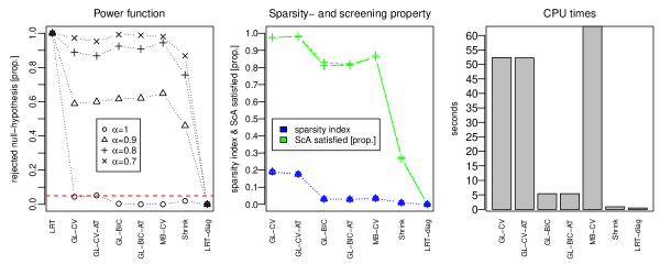
Figure 1: Results Model 1. Performance of DiffNet with different NI approaches and different levels of network concordance ($\alpha$). First panel: Power function (proportion of rejected null-hypothesis). Second panel: In green: proportion of times ScA is satisfied, in blue: sparsity index. Third panel: CPU times. [The different NI methods GL-CV, GL-CV-AT, GL-BIC, GL-BIC-AT, MB-CV and Shrink are described in Table 1. LRT: two-sample likelihood-ratio test for difference between covariance matrices (asymptotic $\chi^{2}_{d\times(d+1)/2}$ null-distribution). LRT-diag: diagonal-restricted two-sample likelihood-ratio test (asymptotic $\chi^{2}_{d}$ distribution)].

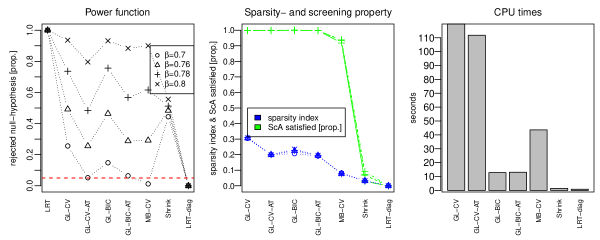
Figure 2: Results Model 2. Same caption as in Figure 1.

3.2 Performance of NetGSA

In this study we simulate data for $S=20$ gene-sets. For each gene-set $s$ we generate data matrices $\mathbf{X}_{s}$ and $\mathbf{Y}_{s}$ from $\mathcal{N}(\mu^{x}_{s},\Sigma^{x}_{s})$ and $\mathcal{N}(\mu^{y}_{s},\Sigma^{y}_{s})$ with $n=n_{x}=n_{y}=40$. The number of genes $d_{s}$ of gene-set $s$ is drawn uniformly from $\{20,\ldots,n-1\}$ ($d_{s}<n$ ensures that the conventional LRT is well-defined). The gene-set specific means, $\mu^{x}_{s}$ and $\mu^{y}_{s}$, are taken to be zero except for the first three gene-sets:

• Gene-set 1: $\mu^{x}_{1}=0$. $\mu^{y}_{1j}=0.2$, $j=1,\ldots,d_{1}$.

• Gene-set 2: $\mu^{x}_{2}=0$. $\mu^{y}_{2j}=0,\;j=1,\ldots,\lceil d_{2}/2\rceil$ and $\mu^{y}_{2j}=0.4,\;j=1,\ldots,\lfloor d_{2}/2\rfloor$.

• Gene-set 3: $\mu^{x}_{3}=0$. $\mu^{y}_{3j}=-0.2,\;j=1,\ldots,\lceil d_{3}/2\rceil$ and $\mu^{y}_{3j}=0.2,\;j=1,\ldots,\lfloor d_{3}/2\rfloor$.

• Gene-sets 4-20: $\mu^{x}_{s}=\mu^{y}_{s}=0$.

All gene-sets have inverse covariance matrices generated as in Model 1. We set $\Omega^{x}_{s}$ and $\Omega^{y}_{s}$ to have $\lceil d_{s}/2\rceil$ non-zero entries at random locations, of which $\alpha_{s}\times\lceil d_{s}/2\rceil$ are common across both conditions. The parameter $\alpha_{s}$ controls relative network concordance and is chosen as:

• Gene-sets 1-3: $\alpha=\alpha_{1}=\alpha_{2}=\alpha_{3}\in\{0,0.25,0.5,1\}.$

• Gene-sets 4-20: $\alpha_{s}=1$, i.e. $\Omega^{x}_{s}=\Omega^{y}_{s}$.

Gene-sets one to three exhibit a difference between conditions in terms of their means. All gene-sets have non-trivial gene networks. By decreasing the parameter $\alpha$ from one to zero we introduce additional network difference for the first three gene-sets .

The aim of this simulation is to investigate performance of NetGSA in detecting gene-sets with network difference between $x$ and $y$. We further want to investigate whether NetGSA can improve overall performance in the setting in which conditions differ with respect to both means and networks. For that purpose we compute p-values using NetGSA; Net(SS) stands for the single-split approach ($B=1$), Net(MS) denotes the multi-split version ($B=50$). We further run a “classical” gene-set analysis using the approach described in Irizarry et al. (2009) (Classic) and combine NetGSA with this approach by reporting the minimum of the two p-values (Classic+Net(MS)). Finally, we compute for each gene-set p-values with the conventional LRT and correct them for multiple comparison (LRT).

Figure 3 shows ROC curves, averaged over $50$ simulation runs, for various levels of relative network concordance $\alpha$. Table 2 shows averaged false discovery and true positive rates at the $5\%$ significance level. As expected performance of NetGSA improves with increasing network difference (smaller $\alpha$ values). We also see that multi-splitting dominates performance compared to using only a single data split. Testing network differences with LRT performs poorly in all scenarios.

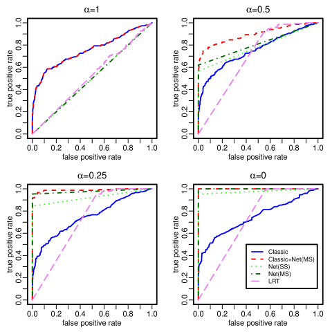
Figure 3: Simulated data, ROC curves. ROC curves show the average true positive rate against the average false positive rate for varying thresholds, where the rates are with respect to gene-sets. Each panel corresponds to a different level of overlap between condition-specific networks, as controlled by a simulation parameter $\alpha$. Upper left panel ($\alpha=1$): no network difference. Upper right panel ($\alpha=0.5$): the two networks for gene-sets 1-3 share half of the edges. Lower left panel ($\alpha=0.25$): the two networks for gene-sets 1-3 share a quarter of the edges. Lower right panel ($\alpha=0$): the two networks for gene-sets 1-3 have no edges in common. [Net(SS): NetGSA with $B=1$ (single-split); Net(MS): NetGSA with $B=50$ (multi-split); Classic: classic gene-set analysis as described in Irizarry et al. (2009); Classic+Net(MS): classic gene-set analysis and NetGSA combined; LRT: conventional likelihood-ratio test.]

	False discovery rate (false positive rate)
	$\alpha=0$	$\alpha=0.25$	$\alpha=0.5$	$\alpha=1$
Classic	0 (0)	0 (0)	0.02 (0.001)	0 (0)
Classic+Net(MS)	0 (0)	0 (0)	0.005 (0.001)	0 (0)
Net(SS)	0 (0)	0 (0)	0 (0)	0 (0)
Net(MS)	0 (0)	0 (0)	0 (0)	0 (0)
LRT	0.851 (0.992)	0.849 (0.994)	0.848 (0.986)	0.848 (0.987)

	True positive rate
	$\alpha=0$	$\alpha=0.25$	$\alpha=0.5$	$\alpha=1$
Classic	0.08	0.113	0.087	0.107
Classic+Net(MS)	0.08	0.447	0.867	1
Net(SS)	0	0.387	0.74	0.953
Net(MS)	0	0.373	0.86	1
LRT	0.987	1	1	1

Table 2: Performance of NetGSA at the $5\%$ significance level. Average false discovery rate (in brackets: false positive rate) and true positive rate at the $5\%$ significance level for various methods and different $\alpha$-values (relative network concordance of gene-set one to three). [Net(SS): NetGSA with $B=1$ (single-split); Net(MS): NetGSA with $B=50$ (multi-split); Classic: classic gene-set analysis as described in Irizarry et al. (2009); Classic+Net(MS): classic gene-set analysis and NetGSA combined; LRT: conventional likelihood-ratio test.]

Calculations in NetGSA are based on Gaussian graphical models and therefore rely upon the normality assumption. In order to investigate performance under deviations from normality we generate data as described above but with $10\%$ of the data contaminated with samples from a multivariate t-distribution (degrees of freedom two and three). We take the $\alpha=0.25$ setup and perform $50$ simulation runs. Figure 4 shows ROC performance of Net(SS), Net(MS) and LRT for the cases with and without t-contamination. As expected performance degrades with more contamination but the effect is not dramatic and performance of NetGSA degrades gradually. However, we also see from Table 3 that the average false discovery rate is larger than expected in presence of t-contamination. Therefore, we recommend to interpret results with care in case of stronger deviation from normality as this could severely increase the number of false discoveries.

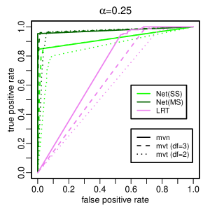
Figure 4: Effect of t-contamination on performance of NetGSA. ROC curves plot the average true positive rate against the average false positive rate for varying thresholds. Solid lines: multivariate normal data (no contamination). Dashed lines: t-contaminated data with degree of freedom df=3. Dotted lines: performance for t-contaminated data with degree of freedom df=2. [Net(SS): NetGSA with $B=1$ (single-split); Net(MS): NetGSA with $B=50$ (multi-split); LRT: conventional likelihood-ratio test.]

	False discovery rate (false positive rate)
	mvn	mvt (df=3)	mvt (df=2)
Net(SS)	0 (0)	0.091 (0.02)	0.299 (0.068)
Net(MS)	0 (0)	0.036 (0.007)	0.17 (0.04)
LRT	0.848 (0.986)	0.85 (0.998)	0.85 (1)

	True positive rate
	mvn	mvt (df=3)	mvt (df=2)
Net(SS)	0.74	0.76	0.74
Net(MS)	0.86	0.873	0.873
LRT	1	1	1

Table 3: Effect of t-contamination on performance of NetGSA at the 5% significance level. Average false discovery rate (in brackets: false positive rate) and true positive rate at the $5\%$ significance level for different levels of t-contamination. mvn: multivariate normal data (no contamination), mvt (df=3): $10\%$ of the data contaminated with samples from a multivariate t-distribution with degrees of freedom df=3, mvt (df=2): $10\%$ of the data contaminated with samples from a multivariate t-distribution with degrees of freedom df=2. [Net(SS): NetGSA with $B=1$ (single-split); Net(MS): NetGSA with $B=50$ (multi-split); LRT: conventional likelihood-ratio test.]

4 Applications

In this Section we apply NetGSA to three datasets from cancer biology. In each application we compare gene expression data between two conditions, using as gene-sets the collection from BioCarta (available at http://www.broadinstitute.org/gsea/msigdb). The latter comprises 216 gene-sets with a number of genes per gene-set which varies from 6 to 87.

Cancer cell line encyclopaedia (CCLE)

We consider the dataset from the Broad-Novartis Cancer Cell Line Encyclopedia (CCLE) (Barretina et al. (2012)). Apart from gene expression levels the CCLE dataset contains also anticancer drug sensitivity measurements. We consider the drug Irinotecan. We focus on the activity area (AA) and extract the numbers of cell lines, $n_{\rm T}$ and $n_{\rm B}$, in the top and bottom third of the AA range. We then define resistant and sensitive cell lines by considering the top $n_{x}=\min\{n_{\rm T},n_{\rm B}\}$ scoring cell lines and the bottom $n_{y}=\min\{n_{\rm T},n_{\rm B}\}$ cell lines (with respect to AA). We compare the resistant against the sensitive cell lines.

Lung cancer

We consider gene expression measurements from large airway epithelial cells sampled from $n_{x}=97$ patients with lung cancer and $n_{y}=90$ controls (Spira et al., 2007). This data was previously analysed with the joint graphical Lasso in Danaher et al. (2013) and it is publicly available at GEO accession number GSE4115. We compare the lung cancer samples against the controls.

Breast cancer

The dataset by Loi et al. (2008) has gene expressions from 255 ER+ breast cancer patients treated with tamoxifen. Using distant metastasis free survival as a primary endpoint, $n_{x}=68$ patients from this dataset are labeled as resistant to tamoxifen and $n_{y}=187$ are labeled as sensitive to tamoxifen and we are interested in differences between these two groups. This dataset is available at GEO accession number GSE6532 and was analysed using the graph-structured tests for differential expression proposed by Jacob et al. (2012).

Our novel approach, NetGSA, is based on the normality assumption. Strong violation from normality can result in a inflated false discovery rate. We therefore conduct Shapiro-Wilk tests for each gene in each condition and discard genes with a p-value (corrected for multiplicity) smaller than 1% in either of the two populations. We run the multi-split version of NetGSA with $B=50$ (Net(MS)) on all three examples, where we normalized the input matrices $\mathbf{X}$ and $\mathbf{Y}$ to have zero mean and variance one. In addition to NetGSA we perform classical GSA (Classic, Irizarry et al. (2009)) on unnormalized data. In all analyses we excluded gene-sets with $d_{s}<5$. Figures 5-7 shows scatter plots of the negative log-p-values obtained with Net(MS) and Classic for the CCLE, the lung cancer and the breast cancer examples. Net(MS) identifies fewer significant gene-sets than Classic. Interestingly, the ordering of gene-sets according to p-values differs substantially for NetGSA and classical GSA. For example in the lung cancer study there are several gene-sets significant under Net(MS) but not under Classic. In order to check that the significant gene-sets are not false positives we perform “back-testing”: in particular we pool data from both populations, randomly divide the data into two populations and then run NetGSA with only the significant gene-sets. We repeat this process ten times. In all examples “back-testing” never declares a gene-set as significant.

In Figures 8 and 10 we show the networks (medians of absolute partial correlation coefficients over 50 random data splits) and a histogram of single-split p-values over the fifty random splits for the top scoring gene-set in each of the three examples.

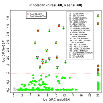
Figure 5: P-value scatter-plots. CCLE dataset, Irinotecan-resistant against -sensitive cell lines. The negative log-p-values obtained using NetGSA and classical GSA are plotted against each other. In green: significant gene-sets using classical GSA; in red: significant gene-sets using NetGSA. At $10\%$ significance level.

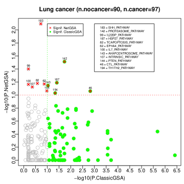
Figure 6: P-value scatter-plots. Lung cancer dataset, lung cancer subjects against control subjects. Same caption as in Figure 5.

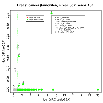
Figure 7: P-value scatter-plots. Breast cancer dataset, Tamoxifen-resistant against -​ sensitive cell lines. Same caption as in Figure 5.

Figure 8: Networks and distribution of single-split p-values. Left and middle panels show heatmaps of the absolute partial correlation coefficients (median over $50$ random data splits) of the top gene-set IL3_PATHWAY for the CCLE (Irinotecan) example. The right panel shows a histogram of the single-split NetGSA p-values for gene-set IL3_PATHWAY over the $50$ random splits.

Figure 9: Networks and distribution of single-split p-values. Left and middle panels show heatmaps of the absolute partial correlation coefficients (median over $50$ random data splits) of the top gene-set SHH_PATHWAY for the lung cancer example. The right panel shows a histogram of the single-split NetGSA p-values for gene-set SHH_PATHWAY over the $50$ random splits.

Figure 10: Networks and distribution of single-split p-values. Left and middle panels show heatmaps of the absolute partial correlation coefficients (median over $50$ random data splits) of the top gene-set IL7_PATHWAY for the breast cancer example. The right panel shows a histogram of the single-split NetGSA p-values for gene-set IL7_PATHWAY over the $50$ random splits.

5 Discussion

The network based gene-set analysis (GSA) procedure we proposed extends gene-set analysis in a multivariate direction. We considered a number of network inference (NI) approaches and on the basis of empirical results and computational considerations suggested the use of Graphical Lasso with adaptive thresholding and tuning parameter set using BIC (“GL-BIC-AT”; see Table 1).

The multivariate nature of our test comes at added computational cost; our approach is far more computationally demanding that a classical, mean-based GSA. Nevertheless, due to the computational efficiency of Graphical Lasso, simplicity of BIC-based setting of the tuning parameters and parallelizability, overall the analysis we propose is efficient and practical on a multicore system. For example, a problem with with $d=1208$ genes and $S=216$ gene-sets took 52 minutes of compute time using 50 cores. We used GGMs to model and test for differences in network structure. However, the high-dimensional two-sample test in Städler and Mukherjee (2013) is very general and NetGSA could be extended to use other graphical models. In particular, directed edges can be appropriate in many biological applications, and extension to the case of directed acyclic graphs (DAGs) would be an interesting avenue for future work. Any such extension would have to carefully consider computational demands, since as discussed above NetGSA requires many rounds of network estimation (albeit far fewer than a naive, permutation alternative).

All our examples considered static (i.e. non-time-varying) data. In many biological applications, time course data play an important role. NetGSA could be used to compare time-course data between conditions by use of a suitable graphical model formulation, such as dynamic Bayesian networks or DBNs (Husmeier, 2003). In the case of (a certain class of) DBNs computationally efficient estimation is possible (Hill et al., 2012), and these models could therefore provide a good starting point for exploring extensions of NetGSA to time-course data. Such a dynamic variant of NetGSA would allow testing of differences between gene-sets based on networks estimated from time course data, and to the extent that time-varying data contain additional information such an approach could offer improved ability to detect biologically relevant differences. Naturally, for such an application sufficient replicates per condition would be needed to obtain p-values, especially via sample splitting.

In principle, given sufficiently many samples, network-based testing could be extended beyond the gene-set level to compare networks over all $d$ variables between conditions. In such a set up gene-sets could be used to constrain estimation of the global network, e.g. allowing more edges within gene-sets than between them. Testing could focus on equality of the overall network, or of subnetworks. NetGSA as proposed here could be regarded as a simplified version of this more general test, in which only within-gene-set edges are allowed.

We considered only gene expression data. However, the methodology could be applied to essentially any molecular data type (including protein and epigenetic), provided suitable sets of variables analogous to gene-sets could be provided. In the case of proteomic data, for example, this could allow testing of differences in protein-protein interplay within known pathways and between conditions.

Acknowledgements: The authors would like to thank Rafael Irizarry for discussion concerning classical gene-set testing. This work was supported in part by NCI U54 CA 112970 and the Cancer Systems Biology Center grant from the Netherlands Organisation for Scientific Research.

References

- Barretina et al. (2012) Barretina, J., Caponigro, G., Stransky, N., Venkatesan, K., Margolin, A. A., Kim, S., Wilson, C. J., Lehár, J., Kryukov, G. V., Sonkin, D., Reddy, A., Liu, M., Murray, L., Berger, M. F., Monahan, J. E., Morais, P., Meltzer, J., Korejwa, A., Jané-Valbuena, J., Mapa, F. A., Thibault, J., Bric-Furlong, E., Raman, P., Shipway, A., Engels, I. H., Cheng, J., Yu, G. K., Yu, J., Aspesi, P., de Silva, M., Jagtap, K., Jones, M. D., Wang, L., Hatton, C., Palescandolo, E., Gupta, S., Mahan, S., Sougnez, C., Onofrio, R. C., Liefeld, T., MacConaill, L., Winckler, W., Reich, M., Li, N., Mesirov, J. P., Gabriel, S. B., Getz, G., Ardlie, K., Chan, V., Myer, V. E., Weber, B. L., Porter, J., Warmuth, M., Finan, P., Harris, J. L., Meyerson, M., Golub, T. R., Morrissey, M. P., Sellers, W. R., Schlegel, R. and Garraway, L. A. (2012) The Cancer Cell Line Encyclopedia enables predictive modelling of anticancer drug sensitivity. Nature, 483, 603–607.
- Danaher et al. (2013) Danaher, P., Wang, P. and Witten, D. (2013) The joint graphical lasso for inverse covariance estimation across multiple classes. To appear in Journal of the Royal Statistical Society, Series B.
- Efron and Tibshirani (2007) Efron, B. and Tibshirani, R. (2007) On testing the significance of sets of genes. Annals of Applied Statistics, 107–129.
- Friedman et al. (2008) Friedman, J., Hastie, T. and Tibshirani, R. (2008) Sparse inverse covariance estimation with the graphical Lasso. Biostatistics, 9, 432–441.
- Hill et al. (2012) Hill, S. M., Lu, Y., Molina, J., Heiser, L. M., Spellman, P. T., Speed, T. P., Gray, J. W., Mills, G. B. and Mukherjee, S. (2012) Bayesian inference of signaling network topology in a cancer cell line. Bioinformatics, 28, 2804–2810.
- Husmeier (2003) Husmeier, D. (2003) Sensitivity and specificity of inferring genetic regulatory interactions from microarray experiments with dynamic bayesian networks. Bioinformatics, 19, 2271–2282.
- Irizarry et al. (2009) Irizarry, R. A., Wang, C., Zhou, Y. and Speed, T. P. (2009) Gene set enrichment analysis made simple. Statistical Methods in Medical Research, 18, 565–575.
- Jacob et al. (2012) Jacob, L., Neuvial, P. and Dudoit, S. (2012) More power via graph-structured tests for differential expression of gene networks. Annals of Applied Statistics, 6, 561–600.
- Jiang and Gentleman (2007) Jiang, Z. and Gentleman, R. (2007) Extensions to gene set enrichment. Bioinformatics, 23, 306–313.
- Krämer et al. (2010) Krämer, N., Schäfer, J. and A.-L., B. (2010) Regularized estimation of large-scale gene regulatory networks with Gaussian graphical models. BMC Bioinformatics, 384.
- Ledoit and Wolf (2004) Ledoit, O. and Wolf, M. (2004) A well-conditioned estimator for large-dimensional covariance matrices. Journal of Multivariate Analysis, 88, 365–411.
- Loi et al. (2008) Loi, S., Haibe-Kains, B., Desmedt, C., Wirapati, P., Lallemand, F., Tutt, A. M., Gillet, C., Ellis, P., Ryder, K., Reid, J. F., Daidone, M. G., Pierotti, M. A., Berns, E. M. M., Jansen, M. P. P., Foekens, J. A., Delorenzi, M., Bontempi, G., Piccart, M. J. and Sotiriou, C. (2008) Predicting prognosis using molecular profiling in estrogen receptor-positive breast cancer treated with tamoxifen. BMC genomics, 9, 239.
- Lönnstedt and Speed (2002) Lönnstedt, I. and Speed, T. (2002) Replicated microarray data. Statistica Sinica, 12, 31–46.
- Meinshausen and Bühlmann (2006) Meinshausen, N. and Bühlmann, P. (2006) High dimensional graphs and variable selection with the Lasso. Annals of Statistics, 34, 1436–1462.
- Meinshausen et al. (2009) Meinshausen, N., Meier, L. and Bühlmann, P. (2009) P-values for high-dimensional regression. Journal of the American Statistical Association, 104, 1671–1681.
- Schäfer and Strimmer (2005) Schäfer, J. and Strimmer, K. (2005) A Shrinkage Approach to Large-Scale Covariance Matrix Estimation and Implications for Functional Genomics. Statistical Applications in Genetics and Molecular Biology, 4.
- Smyth (2004) Smyth, G. K. (2004) Linear models and empirical bayes methods for assessing differential expression in microarray experiments. Statistical Applications in Genetics and Molecular Biology, 3.
- Spira et al. (2007) Spira, A., Beane, J. E., Shah, V., Steiling, K., Liu, G., Schembri, F., Gilman, S., Dumas, Y.-M., Calner, P., Sebastiani, P., Sridhar, S., Beamis, J., Lamb, C., Anderson, T., Gerry, N., Keane, J., Lenburg, M. E. and Brody, J. S. (2007) Airway epithelial gene expression in the diagnostic evaluation of smokers with suspect lung cancer. Nature Medicine, 13, 361–366.
- Städler and Mukherjee (2013) Städler, N. and Mukherjee, S. (2013) Two-sample testing in high-dimensional models. arXiv:1210.4584.
- Subramanian et al. (2005) Subramanian, A., Tamayo, P., Mootha, V. K., Mukherjee, S., Ebert, B. L., Gillette, M. A., Paulovich, A., Pomeroy, S. L., Golub, T. R., Lander, E. S. and Mesirov, J. P. (2005) Gene set enrichment analysis: a knowledge-based approach for interpreting genome-wide expression profiles. Proceedings of the National Academy of Sciences of the United States of America, 102, 15545–15550.
- Tibshirani (1996) Tibshirani, R. (1996) Regression shrinkage and selection via the Lasso. Journal of the Royal Statistical Society, Series B, 58, 267–288.
- Tusher et al. (2001) Tusher, V. G., Tibshirani, R. and Chu, G. (2001) Significance analysis of microarrays applied to the ionizing radiation response. Proceedings of the National Academy of Sciences of the United States of America, 98, 5116–5121.
- van de Wiel et al. (2009) van de Wiel, M. A., Berkhof, J. and van Wieringen, W. N. (2009) Testing the prediction error difference between 2 predictors. Biostatistics, 10, 550–60.
- Wasserman and Roeder (2009) Wasserman, L. and Roeder, K. (2009) High-dimensional variable selection. Annals of Statistics, 37, 2178–2201.
- Yuan and Lin (2007) Yuan, M. and Lin, Y. (2007) Model selection and estimation in the Gaussian graphical model. Biometrika, 94, 19–35.