Closed-Loop Beam Alignment for Massive MIMO Channel Estimation

Abstract

Training sequences are designed to probe wireless channels in order to obtain channel state information for block-fading channels. Optimal training sounds the channel using orthogonal beamforming vectors to find an estimate that optimizes some cost function, such as mean square error. As the number of transmit antennas increases, however, the training overhead becomes significant. This creates a need for alternative channel estimation schemes for increasingly large transmit arrays. In this work, we relax the orthogonal restriction on sounding vectors. The use of a feedback channel after each forward channel use during training enables closed-loop sounding vector design. A misalignment cost function is introduced, which provides a metric to sequentially design sounding vectors. In turn, the structure of the sounding vectors aligns the transmit beamformer with the true channel direction, thereby increasing beamforming gain. This beam alignment scheme for massive MIMO is shown to improve beamforming gain over conventional orthogonal training for a MISO channel.

I Introduction

In wireless communications, accurate channel state information plays a central role in realizing the gains afforded by coherent communications. In light of this, much literature exists to design training sequences to estimate the channel. For a block-fading channel model, [1] addressed capacity maximizing values for various parameters, including the length of the training phase and the power of the training phase. The error covariance of the minimum mean square error (MMSE) channel estimate is minimized when orthogonal waveforms are transmitted from each element. For orthogonal transmission from each element, the discrete length of the training signal must be at least equal to the number of transmit antennas. For massive MIMO systems, this would lead to training consuming a large fraction of the coherence interval.

Channel estimation with training sequences of length less than the number of transmit antennas was considered for distributed transmit beamforming systems in [2]. The set of training sequences which minimizes the mean square error of the MMSE channel estimate was shown to be similar to those maximizing the expected beamforming gain, which gives a training signal matrix with orthogonal columns. The optimal full-rank set of receive beamforming vectors for angle of arrival estimation was derived in [3]. The channel gain term was treated as a deterministic unknown, and beamforming vectors were derived to minimize the variance on the angle of arrival estimate.

The literature referenced thus far in this work pertains to a class of open loop schemes in which the training sequence is predetermined. These training sequences cannot be adapted to knowledge gathered of the instantaneous channel. Alternatively, adaptive training schemes use a feedback link from the receiver to the transmitter to guide the design of the training sequence. Closed-loop training across multiple blocks for massive MIMO beamforming systems is considered in [4]. Assuming a temporally correlated channel, their algorithm selected the entire training signal for a given block based on channel estimates from previous blocks. Improvements in average receive SNR were shown by utilizing the training sequences received in previous channel blocks. Line-of-sight channel estimation for large arrays in backhaul cellular networks is presented in [5]. Adaptive subspace sampling, where samples from previous channel uses aid in beamformer design, gave improved beamforming gain over non-adaptive techniques.

In this work, we focus on channel estimation for single-user massive MIMO. These techniques can be extended to multiuser scenarios, a topic of future work. As the number of antennas grows large, optimal channel estimation no longer remains practical. Some of the general properties for massive MIMO systems were shown to hold for arrays between $100$ and $1,000$ antennas in [6]. We target practical massive MIMO systems and develop a beam alignment scheme to estimate MISO channels on the lower end of that range. We consider beamforming for a MISO channel in a single coherent channel block. A feedback channel allows adaptation of the training sequence after each channel use. In general, current systems do not feed back information after every channel use. The increased complexity, however, may become necessary for massive MIMO systems to shorten the training phase. The training sequence is comprised of sounding vectors, which are sequentially designed in a manner that aligns the estimated channel with the true instantaneous channel direction, treating the channel gain term as a nuisance parameter. This work focuses on frequency division duplexing (FDD) systems, where channel reciprocity cannot be used for transmit beamforming. Nonetheless, this scheme remains applicable for time division duplexing (TDD) systems with no uplink sounding.

II System Setup

Consider a multiple-input single-output (MISO) wireless channel with $M$ transmit antennas and a single receive antenna. In coherent communications, the wireless channel is considered known and knowledge of the channel at the receiver aids symbol detection and demodulation. For a given channel use, the input-output relationship is

$$r=\left(\sqrt{\rho}{\mathbf{x}}\right)^{*}\left(\alpha{\mathbf{h}}\right)+n$$

where ${\mathbf{x}}\in\mathbb{C}^{M\times 1}$ is the transmitted signal with $E\left[\lVert{\mathbf{x}}\rVert^{2}\right]=1$, $\rho$ denotes the transmit power, $r\in\mathbb{C}$ is the received signal, $n\sim\mathcal{CN}(0,\sigma^{2}_{n})$ the additive noise, $(\cdot)^{*}$ denotes the Hermitian transpose, and $\alpha{\mathbf{h}}$ is the MISO wireless channel, comprised of the complex scalar channel gain $\alpha$ and the channel direction vector ${\mathbf{h}}$ with $\lVert{\mathbf{h}}\rVert=1$. The channel direction vector ${\mathbf{h}}$ describes direction only and lacks any sort of gain or attenuation.

Transmit beamforming is commonly used in point-to-point MISO systems, but it is also expected to be critical to multiuser massive MIMO systems. A beamformed transmit signal is defined as ${\mathbf{x}}={\mathbf{f}}s$, where the beamforming vector ${\mathbf{f}}$ and complex symbol $s$ are constrained to $\lVert{\mathbf{f}}\rVert=1$ and $E[\lvert s\rvert^{2}]=1$. The input-output relationship then simplifies to $r=\sqrt{\rho}\alpha({\mathbf{f}}^{*}{\mathbf{h}})s+n$, where $\lvert{\mathbf{f}}^{*}{\mathbf{h}}\rvert^{2}$ denotes the beamforming gain. The optimal beamformer ${\mathbf{f}}_{\text{opt}}$ that maximizes the beamforming gain and achieves $\lvert{\mathbf{f}}_{\text{opt}}^{*}{\mathbf{h}}\rvert^{2}=1$ is ${\mathbf{f}}_{\text{opt}}={\mathbf{h}}$. However, the true channel direction ${\mathbf{h}}$ is unknown and must be estimated.

To estimate the wireless channel, assume $K$ channel uses are available for this task. If the transmit signal for data transmission is restricted to beamforming, it is natural to restrict the training signal in the same fashion. Let the sounding vector ${\mathbf{w}}_{k}$ represent the training signal for the ${k^{\text{th}}}$ channel use. The receive vector for the first $k$ channel uses of the training phase is given by

$${\mathbf{y}}_{k}=\alpha\sqrt{\rho}{\mathbf{W}}_{k}^{*}{\mathbf{h}}+{\mathbf{n}}_{k}$$ (1)

where ${\mathbf{W}}_{k}=[{\mathbf{w}}_{1},{\mathbf{w}}_{2},\ldots,{\mathbf{w}}_{k}]$ is the set of $k$ sounding vectors and ${\mathbf{y}}_{k}$ is the $k\times 1$ complex receive sample vector.

To aid in channel estimation, we consider a limited-rate feedback channel from the receiver to the transmitter as shown in Fig. 1. Let $\mathcal{W}$ represent the set of possible sounding vectors, $\mathcal{W}=\{{\mathbf{w}}^{(\ell)}\in\mathbb{C}^{M\times 1}:\lVert{\mathbf{w}}^{(\ell)}\rVert=1,\ell=1,\ldots,L\}$. Due to the restricted bandwidth of the feedback channel, we design $\mathcal{W}$ to be a discrete set with $\lvert\mathcal{W}\rvert=L$, where $\lvert\mathcal{W}\rvert$ denotes the cardinality of the set $\mathcal{W}$, and make this codebook available ahead of time to both the transmitter and receiver. For the ${k^{\text{th}}}$ channel use, the receiver calculates an estimate of ${\mathbf{h}}$ and decides on the appropriate ${\mathbf{w}}^{(\ell)}\in\mathcal{W}$ to sound the ${(k+1)^{\text{th}}}$ channel use. The index of this sounding vector is fed back to the transmitter, as described in Fig. 1. Note the feedback link is utilized after every channel use during training, which differs from previous channel estimation schemes, including [4]. This creates considerable feedback overhead per coherence time, which is the tradeoff for fewer pilots.

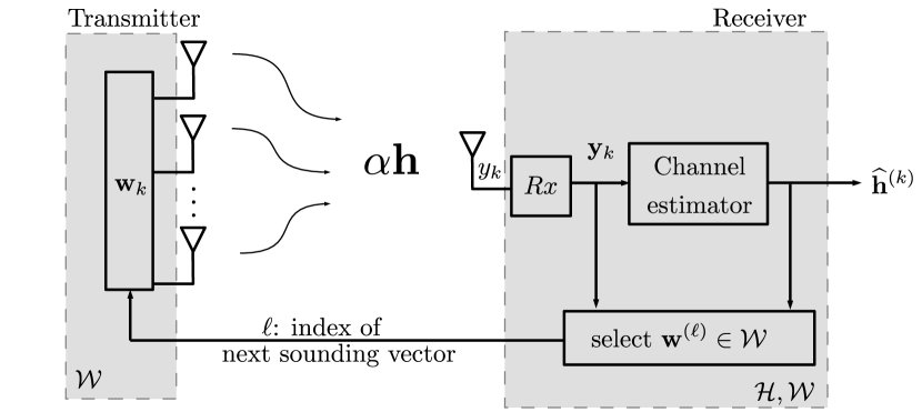
Figure 1: Block diagram illustrating the proposed training scheme. The receiver selects the sounding vector from the codebook $\mathcal{W}$ for the next channel use and feeds back the codeword index to the transmitter.

Assume the channel direction vector belongs to a discrete set ${\mathcal{H}}$. In practice, ${\mathcal{H}}$ approximates the true channel subspace. The maximum likelihood channel estimator is given as,

$$\widehat{{\mathbf{h}}}^{(k)} = \mathop{\mathrm{argmax}}_{{\mathbf{h}}\in\mathcal{H}}p\left({\mathbf{y}}_{k}|{\mathbf{h}},{\mathbf{W}}_{k},\alpha\right)$$

$$= \mathop{\mathrm{argmin}}_{{\mathbf{h}}\in\mathcal{H}}\lVert{\mathbf{y}}_{k}-\alpha\sqrt{\rho}{\mathbf{W}}_{k}^{*}{\mathbf{h}}\rVert^{2}$$

Given this channel direction estimator, after $K$ channel uses of training the beamforming vector for data transmission is set to ${\mathbf{f}}=\widehat{{\mathbf{h}}}^{(K)}$.

In addition to estimating the channel direction, the channel gain term $\alpha$ must also be estimated. We treat $\alpha$ as a nuisance parameter and resort to composite estimation techniques. A generalized maximum likelihood estimator replaces the true channel gain by its maximum likelihood estimate,

$$\widehat{\alpha}_{{\mathbf{h}}} = \mathop{\mathrm{argmax}}_{\alpha\in\mathbb{C}}p\left({\mathbf{y}}_{k}|{\mathbf{h}},{\mathbf{W}}_{k},\alpha\right)=\frac{{\mathbf{h}}^{*}{\mathbf{W}}_{k}{\mathbf{y}}_{k}}{\sqrt{\rho}\lVert{\mathbf{W}}^{*}_{k}{\mathbf{h}}\rVert^{2}}.$$

This result can be shown by minimizing the squared norm $\lVert{\mathbf{y}}_{k}-\alpha\sqrt{\rho}{\mathbf{W}}_{k}^{*}{\mathbf{h}}\rVert^{2}$ over all $\alpha\in\mathbb{C}$. We write the channel magnitude as a complex scalar to incorporate the phase invariance of the channel direction estimate. Beamforming gain is invariant to the phase of the channel direction, e.g., $e^{j\phi}\widehat{{\mathbf{h}}}^{(k)}$ and $\widehat{{\mathbf{h}}}^{(k)}$ give the same beamforming gain. If ${\mathcal{H}}$ is a discrete set, a given ${\mathbf{h}}\in{\mathcal{H}}$ could provide large beamforming gain but give a low likelihood due to its phase. This issue is resolved if we consider $\alpha$ to be complex. The generalized ML channel estimator is given by substituting $\widehat{\alpha}_{{\mathbf{h}}}$ into $p({\mathbf{y}}_{k}|{\mathbf{h}},{\mathbf{W}}_{k},\alpha)$,

$$\widehat{{\mathbf{h}}}^{(k)} = \mathop{\mathrm{argmax}}_{{\mathbf{h}}\in\mathcal{H}}\frac{\lvert{\mathbf{y}}_{k}^{*}{\mathbf{W}}_{k}^{*}{\mathbf{h}}\rvert^{2}}{\lVert{\mathbf{W}}_{k}^{*}{\mathbf{h}}\rVert^{2}}=\mathop{\mathrm{argmax}}_{{\mathbf{h}}\in\mathcal{H}}d_{k}({\mathbf{h}})$$ (2)

where $d_{k}({\mathbf{h}})=\frac{\lvert{\mathbf{y}}_{k}^{*}{\mathbf{W}}_{k}^{*}{\mathbf{h}}\rvert^{2}}{\lVert{\mathbf{W}}_{k}^{*}{\mathbf{h}}\rVert^{2}}$. In essence, this channel estimator finds the channel vector ${\mathbf{h}}\in\mathcal{H}$ whose projection onto ${\mathbf{W}}_{k}$ most closely aligns with the direction of ${\mathbf{y}}_{k}$. The normalizing term $\lVert{\mathbf{W}}_{k}^{*}{\mathbf{h}}\rVert^{2}$ removes any dependence on vector magnitude. If one interprets each ${\mathbf{h}}\in{\mathcal{H}}$ as a beam, the channel estimator selects the beam whose projection onto ${\mathbf{W}}_{k}$ most closely aligns with ${\mathbf{y}}_{k}$. Beam alignment is performed by properly selecting successive sounding vectors.

III Sounding Vector Selection

As one might expect, the sounding vectors have direct influence on the performance of the channel estimator in (2). In this section, we address how to select the sounding vector for each channel use. With feedback after every channel use, the sounding vector for the ${(k+1)^{\text{th}}}$ channel use can be chosen as a function of the previous $k$ receive samples, ${\mathbf{y}}_{k}$. Let us define the misalignment event after $k+1$ channel uses as ${\mathcal{M}}_{i}=\big{\{}\widehat{{\mathbf{h}}}^{(k+1)}\neq{\mathbf{h}}\big{|}{\mathbf{y}}_{k},{\mathbf{W}}_{k+1},{\mathbf{h}}={\mathbf{h}}_{i},\widehat{\alpha}_{{\mathbf{h}}_{i}}\big{\}}$. This misalignment event occurs when the estimated channel direction $\widehat{{\mathbf{h}}}^{(k+1)}$ is not the true channel direction ${\mathbf{h}}={\mathbf{h}}_{i}$. Averaging the probability of the misalignment event over all channel directions gives the misalignment cost function for the ${(k+1)^{\text{th}}}$ channel use evaluated at channel use $k$,

$$\halign to=0.0pt{\relax\global\advance\@IEEEeqncolcnt by 1\relax\begingroup\csname @IEEEeqnarraycolPREr\endcsname#\relax\relax\relax\relax\relax\relax\relax\relax\relax\relax\csname @IEEEeqnarraycolPOSTr\endcsname\relax\relax\relax\relax\relax\relax\relax\relax\relax\relax\endgroup&\relax\global\advance\@IEEEeqncolcnt by 1\relax\begingroup\csname @IEEEeqnarraycolPREC\endcsname#\relax\relax\relax\relax\relax\relax\relax\relax\relax\relax\csname @IEEEeqnarraycolPOSTC\endcsname\relax\relax\relax\relax\relax\relax\relax\relax\relax\relax\endgroup&\relax\global\advance\@IEEEeqncolcnt by 1\relax\begingroup\csname @IEEEeqnarraycolPREl\endcsname#\relax\relax\relax\relax\relax\relax\relax\relax\relax\relax\csname @IEEEeqnarraycolPOSTl\endcsname\relax\relax\relax\relax\relax\relax\relax\relax\relax\relax\endgroup&\global\advance\@IEEEeqncolcnt by 1\relax\bgroup#\egroup&\global\advance\@IEEEeqncolcnt by 1\relax\hbox to\z@\bgroup\hss#\egroup\cr$\displaystyle {$P^{\text{mis}}_{k+1|k}({\mathbf{w}}_{k+1})$}= \sum_{i=1}^{N} \text{Pr} ({\mathcal{M}}_{i}) p_{i}^{(k)} $\hfil&{{}\vrule width=0.0pt,height=0.0pt,depth=0.0pt}&0.0pt{\hss{\normalcolor(3)}}\cr\penalty 100\vskip 3.0pt\vskip 0.0pt\cr\hfil$\displaystyle\qquad$&\hfil$\displaystyle{}={}$\hfil&$\displaystyle\sum_{i=1}^{N} \text{Pr} \bigg{(} d_{k+1}({\mathbf{h}}_{i}) < \text{max} \Big{[} \big{\{} d_{k+1}({\mathbf{h}}_{j}) \big{\}}_{j \neq i} \Big{]} \Big{|}{\mathcal{V}}_{i} \bigg{)} p_{i}^{(k)} $\hfil&{\vrule width=0.0pt,height=0.0pt,depth=0.0pt}&0.0pt{\hss{\normalcolor(4)}}\cr}$$

where $p_{i}^{(k)}=p({\mathbf{h}}_{i}|{\mathbf{y}}_{k},{\mathbf{W}}_{k},\widehat{\alpha}_{{\mathbf{h}}_{i}})$ are the updated priors after $k$ channel uses and ${\mathcal{V}}_{i}=\{{\mathbf{h}}={\mathbf{h}}_{i},{\mathbf{y}}_{k},{\mathbf{W}}_{k},\widehat{\alpha}_{{\mathbf{h}}_{i}}\}$. This cost function measures the penalty of choosing the wrong channel direction as a function of ${\mathbf{w}}_{k+1}$. The previous $k$ receive samples are known, and the receive sample for the ${(k+1)^{\text{th}}}$ channel use, $y_{k+1}$, is treated as a random variable as described in Section III-A. In what follows, the misalignment cost function is adopted to develop a sounding vector selection criterion.

III-A Binary Channel Codebook

We approximate, in this subsection, the channel using a binary channel codebook, ${\mathcal{H}}=\{{\mathbf{h}}_{1},{\mathbf{h}}_{2}\}$. Despite being an extremely coarse discretization of the channel space, the exact misalignment cost function can be derived for the binary codebook case,

$$\halign to=0.0pt{\relax\global\advance\@IEEEeqncolcnt by 1\relax\begingroup\csname @IEEEeqnarraycolPREr\endcsname#\relax\relax\relax\relax\relax\relax\relax\relax\relax\relax\csname @IEEEeqnarraycolPOSTr\endcsname\relax\relax\relax\relax\relax\relax\relax\relax\relax\relax\endgroup&\relax\global\advance\@IEEEeqncolcnt by 1\relax\begingroup\csname @IEEEeqnarraycolPREC\endcsname#\relax\relax\relax\relax\relax\relax\relax\relax\relax\relax\csname @IEEEeqnarraycolPOSTC\endcsname\relax\relax\relax\relax\relax\relax\relax\relax\relax\relax\endgroup&\relax\global\advance\@IEEEeqncolcnt by 1\relax\begingroup\csname @IEEEeqnarraycolPREl\endcsname#\relax\relax\relax\relax\relax\relax\relax\relax\relax\relax\csname @IEEEeqnarraycolPOSTl\endcsname\relax\relax\relax\relax\relax\relax\relax\relax\relax\relax\endgroup&\global\advance\@IEEEeqncolcnt by 1\relax\bgroup#\egroup&\global\advance\@IEEEeqncolcnt by 1\relax\hbox to\z@\bgroup\hss#\egroup\cr\hfil$\displaystyle{$P^{\text{mis}}_{k+1|k}({\mathbf{w}}_{k+1})$}$&\hfil$\displaystyle{}={}$\hfil&$\displaystyle\text{Pr} \Big{(} d_{k+1}({\mathbf{h}}_{1}) < d_{k+1}({\mathbf{h}}_{2}) \Big{|}{\mathcal{V}}_{1} \Big{)} p_{1}^{(k)} $\hfil&{{}\vrule width=0.0pt,height=0.0pt,depth=0.0pt&0.0pt{\hss{\normalcolor(5)}}\cr\penalty 100\vskip 3.0pt\vskip 0.0pt\cr}&+\,\,\text{Pr}\Big{(}d_{k+1}({\mathbf{h}}_{2})<d_{k+1}({\mathbf{h}}_{1})\Big{|}{\mathcal{V}}_{2}\Big{)}p_{2}^{(k)}\vrule width=0.0pt,height=0.0pt,depth=0.0pt\cr}$$

which is the weighted sum of pairwise error probability (PEP) terms. The $\text{PEP}\left({\mathbf{h}}_{2}\rightarrow{\mathbf{h}}_{1}\right|{\mathcal{V}}_{2})$ is the probability ${\mathbf{h}}_{1}$ is chosen assuming ${\mathbf{h}}_{2}$ is true,

$$\halign to=0.0pt{\relax\global\advance\@IEEEeqncolcnt by 1\relax\begingroup\csname @IEEEeqnarraycolPREl\endcsname#\relax\relax\relax\relax\relax\relax\relax\relax\relax\relax\csname @IEEEeqnarraycolPOSTl\endcsname\relax\relax\relax\relax\relax\relax\relax\relax\relax\relax\endgroup&\relax\global\advance\@IEEEeqncolcnt by 1\relax\begingroup\csname @IEEEeqnarraycolPREr\endcsname#\relax\relax\relax\relax\relax\relax\relax\relax\relax\relax\csname @IEEEeqnarraycolPOSTr\endcsname\relax\relax\relax\relax\relax\relax\relax\relax\relax\relax\endgroup&\global\advance\@IEEEeqncolcnt by 1\relax\bgroup#\egroup&\global\advance\@IEEEeqncolcnt by 1\relax\hbox to\z@\bgroup\hss#\egroup\cr$\displaystyle\text{PEP}\left( {\mathbf{h}}_{2} \rightarrow{\mathbf{h}}_{1} \right|{\mathcal{V}}_{2}) = $\hfil&\hfil$\displaystyle{}$&{\vrule width=0.0pt,height=0.0pt,depth=0.0pt}&0.0pt{\hss{\normalcolor(6)}}\cr\penalty 100\vskip 3.0pt\vskip 0.0pt\cr$\displaystyle\quad\quad\text{Pr} \left( \frac{\lvert{\mathbf{y}}_{k+1}^{*} {\mathbf{W}}_{k+1}^{*} {\mathbf{h}}_{1}\rvert^{2}}{\lVert{\mathbf{W}}_{k+1}^{*} {\mathbf{h}}_{1}\rVert^{2}} > \frac{\lvert{\mathbf{y}}_{k+1}^{*} {\mathbf{W}}_{k+1}^{*} {\mathbf{h}}_{2}\rvert^{2}}{\lVert{\mathbf{W}}_{k+1}^{*} {\mathbf{h}}_{2}\rVert^{2}} \Bigg{|}{\mathcal{V}}_{2} \right). $\hfil&\hfil$\displaystyle$&{\vrule width=0.0pt,height=0.0pt,depth=0.0pt}&0.0pt{\hss}\cr}$$

Since $\frac{{\mathbf{y}}_{k+1}^{*}{\mathbf{W}}_{k+1}^{*}{\mathbf{h}}_{i}}{\lVert{\mathbf{W}}_{k+1}^{*}{\mathbf{h}}_{i}\rVert}$ is a Gaussian random variable when conditioned on ${\mathbf{h}}_{i}$, the pairwise error probability is the probability the magnitude of one Gaussian random variable exceeds the magnitude of another. We now calculate the PEP considering $d_{k+1}({\mathbf{h}}_{1})$ and $d_{k+1}({\mathbf{h}}_{2})$ are functions of the same scalar noise term, $n_{k+1}$.

Lemma 1.

Consider two Gaussian random variables,

$$X = \mu_{x}+q_{x}n\sim\mathcal{CN}(\mu_{x},\lvert q_{x}\rvert^{2})$$

$$Y = \mu_{y}+q_{y}n\sim\mathcal{CN}(\mu_{y},\lvert q_{y}\rvert^{2})$$

where $\mu_{x},\mu_{y},q_{x},q_{y}$ are all constant complex scalars and $n\sim\mathcal{CN}(0,1)$. Then,

$$\halign to=0.0pt{\relax\global\advance\@IEEEeqncolcnt by 1\relax\begingroup\csname @IEEEeqnarraycolPREr\endcsname#\relax\relax\relax\relax\relax\relax\relax\relax\relax\relax\csname @IEEEeqnarraycolPOSTr\endcsname\relax\relax\relax\relax\relax\relax\relax\relax\relax\relax\endgroup&\relax\global\advance\@IEEEeqncolcnt by 1\relax\begingroup\csname @IEEEeqnarraycolPREl\endcsname#\relax\relax\relax\relax\relax\relax\relax\relax\relax\relax\csname @IEEEeqnarraycolPOSTl\endcsname\relax\relax\relax\relax\relax\relax\relax\relax\relax\relax\endgroup&\global\advance\@IEEEeqncolcnt by 1\relax\bgroup#\egroup&\global\advance\@IEEEeqncolcnt by 1\relax\hbox to\z@\bgroup\hss#\egroup\cr$\displaystyle\text{Pr}\left( \lvert X\rvert^{2} > \lvert Y\rvert^{2} \right) = $\hfil&{{}\vrule width=0.0pt,height=0.0pt,depth=0.0pt}&0.0pt{\hss{\normalcolor(7)}}\cr\penalty 100\vskip 3.0pt\vskip 0.0pt\cr\hfil$\displaystyle\qquad\begin{cases}1 -Q_{1}\left( \left|\frac{\mu_{y} q_{y}^{*} - \mu_{x} q_{x}^{*}}{\lvert q_{y}\rvert^{2}-\lvert q_{x}\rvert^{2}} \right|, \left|\frac{\mu_{x} q_{y} - q_{x} \mu_{y}}{\lvert q_{y}\rvert^{2}-\lvert q_{x}\rvert^{2}} \right|\right) &\text{ \emph{if} } \lvert q_{y}\rvert^{2} > \lvert q_{x}\rvert^{2}\\ Q_{1}\left( \left|\frac{\mu_{y} q_{y}^{*} - \mu_{x} q_{x}^{*}}{\lvert q_{y}\rvert^{2}-\lvert q_{x}\rvert^{2}} \right|, \left|\frac{\mu_{x} q_{y} - q_{x} \mu_{y}}{\lvert q_{y}\rvert^{2}-\lvert q_{x}\rvert^{2}} \right|\right) &\text{ if } \lvert q_{y}\rvert^{2} < \lvert q_{x}\rvert^{2}\\ \frac{1}{2} \left[ 1 + \text{\emph{erf}} \left( \frac{\lvert\mu_{y}\rvert^{2}-\lvert\mu_{x}\rvert^{2}}{2\sqrt{2}\lvert\mu_{y}^{*} q_{y} - \mu_{x}^{*} q_{x}\rvert} \right) \right] &\text{ if } \lvert q_{y}\rvert^{2} = \lvert q_{x}\rvert^{2}\end{cases} $&$\displaystyle$\hfil&{\vrule width=0.0pt,height=0.0pt,depth=0.0pt}&0.0pt{\hss{\normalcolor(8)}}\cr}$$

where $Q_{1}(\cdot,\cdot)$ is the first-order Marcum Q function [7].

Proof:

See Appendix. ∎

Assuming ${\mathbf{h}}_{2}$ is true, the pairwise error probability in (III-A) is calculated using Lemma 1 by setting $\mu_{x}=\frac{{\mathbf{y}}_{k}^{*}{\mathbf{W}}_{k}^{*}{\mathbf{h}}_{1}+\sqrt{\rho}\widehat{\alpha}_{{\mathbf{h}}_{2}}^{*}{\mathbf{h}}_{2}^{*}{\mathbf{w}}_{k+1}{\mathbf{w}}_{k+1}^{*}{\mathbf{h}}_{1}}{\lVert{\mathbf{W}}_{k+1}^{*}{\mathbf{h}}_{1}\rVert}$, $q_{x}=\frac{{\mathbf{w}}_{k+1}^{*}{\mathbf{h}}_{1}}{\lVert{\mathbf{W}}_{k+1}^{*}{\mathbf{h}}_{1}\rVert}$, $\mu_{y}=\frac{{\mathbf{y}}_{k}^{*}{\mathbf{W}}_{k}^{*}{\mathbf{h}}_{2}+\sqrt{\rho}\widehat{\alpha}_{{\mathbf{h}}_{2}}^{*}\lvert{\mathbf{w}}_{k+1}^{*}{\mathbf{h}}_{2}\rvert^{2}}{\lVert{\mathbf{W}}_{k+1}^{*}{\mathbf{h}}_{2}\rVert}$, and $q_{y}=\frac{{\mathbf{w}}_{k+1}^{*}{\mathbf{h}}_{2}}{\lVert{\mathbf{W}}_{k+1}^{*}{\mathbf{h}}_{2}\rVert}$.

The sounding vector for the next channel use is chosen as,

$${\mathbf{w}}_{k+1}=\mathop{\mathrm{argmin}}_{{\mathbf{w}}^{(\ell)}\in\mathcal{W}}P^{\text{mis}}_{k+1|k}({\mathbf{w}}^{(\ell)})$$ (9)

III-B N-ary Channel Codebook

We now extend our scope to the $N$-ary scenario. Let $\mathcal{H}=\{{\mathbf{h}}_{1},\,{\mathbf{h}}_{2},\,\ldots,\,{\mathbf{h}}_{N}\}$. The misalignment cost function expression in (III) cannot be simplified in terms of the pairwise error probabilities, as was the case for the binary channel codebook. Using a union bound argument, we can place an upper bound on the misalignment cost function

$${P^{\text{mis}}_{k+1|k}({\mathbf{w}}_{k+1})}\leq\sum_{i=1}^{N}\sum_{\begin{subarray}{c}j=1\\ j\neq i\end{subarray}}^{N}\text{PEP}\left({\mathbf{h}}_{i}\rightarrow{\mathbf{h}}_{j}|{\mathcal{V}}_{i}\right)p_{i}^{(k)}.$$ (10)

Calculating the misalignment cost function requires evaluating $\lvert{\mathcal{H}}\rvert(\lvert{\mathcal{H}}\rvert-1)$ PEP terms for each sounding vector codeword in ${\mathcal{W}}$. For larger codebooks, the complexity of this algorithm becomes significant, as $\lvert{\mathcal{H}}\rvert(\lvert{\mathcal{H}}\rvert-1)\lvert{\mathcal{W}}\rvert$ PEP terms must be calculated for each channel use.

III-C Low Complexity Beam Alignment

In general, the size of the channel codebook and sounding vector codebook scales with the number of transmit antennas to maintain a fixed quantization error. As a result, the complexity to select a sounding vector at each channel use will scale with $M$. To make the beam alignment algorithm tractable for moderately sized arrays, we approximate (10). To do this, we note that as the number of channel uses increases, the beam alignment algorithm typically prefers a single codeword corresponding to a high $p_{i}^{(k)}$. Based on this observation, we can simplify the misalignment cost function to only consider the two most likely codewords. Letting ${\mathbf{h}}_{(1)}$ represent the most likely channel codeword and ${\mathbf{h}}_{(2)}$ represent the second most likely channel codeword, we can approximate (10) as

$$\halign to=0.0pt{\relax\global\advance\@IEEEeqncolcnt by 1\relax\begingroup\csname @IEEEeqnarraycolPREr\endcsname#\relax\relax\relax\relax\relax\relax\relax\relax\relax\relax\csname @IEEEeqnarraycolPOSTr\endcsname\relax\relax\relax\relax\relax\relax\relax\relax\relax\relax\endgroup&\relax\global\advance\@IEEEeqncolcnt by 1\relax\begingroup\csname @IEEEeqnarraycolPREC\endcsname#\relax\relax\relax\relax\relax\relax\relax\relax\relax\relax\csname @IEEEeqnarraycolPOSTC\endcsname\relax\relax\relax\relax\relax\relax\relax\relax\relax\relax\endgroup&\relax\global\advance\@IEEEeqncolcnt by 1\relax\begingroup\csname @IEEEeqnarraycolPREl\endcsname#\relax\relax\relax\relax\relax\relax\relax\relax\relax\relax\csname @IEEEeqnarraycolPOSTl\endcsname\relax\relax\relax\relax\relax\relax\relax\relax\relax\relax\endgroup&\global\advance\@IEEEeqncolcnt by 1\relax\bgroup#\egroup&\global\advance\@IEEEeqncolcnt by 1\relax\hbox to\z@\bgroup\hss#\egroup\cr\hfil$\displaystyle{$P^{\text{mis}}_{k+1|k}({\mathbf{w}}_{k+1})$}$&\hfil$\displaystyle{}\approx{}$\hfil&$\displaystyle\text{PEP}\left( {\mathbf{h}}_{(1)} \rightarrow{\mathbf{h}}_{(2)} |{\mathcal{V}}_{(1)} \right) p_{(1)}^{(k)} $\hfil&{{}\vrule width=0.0pt,height=0.0pt,depth=0.0pt&0.0pt{\hss}\cr\penalty 100\vskip 3.0pt\vskip 0.0pt\cr}&\quad+\,\,\text{PEP}\left({\mathbf{h}}_{(2)}\rightarrow{\mathbf{h}}_{(1)}|{\mathcal{V}}_{(2)}\right)p_{(2)}^{(k)}.\vrule width=0.0pt,height=0.0pt,depth=0.0pt\cr}$$

In this manner, the beam alignment algorithm calculates $2\lvert{\mathcal{W}}\rvert$ PEP terms, a significant reduction from the union bound which calculates $\lvert{\mathcal{H}}\rvert(\lvert{\mathcal{H}}\rvert-1)\lvert{\mathcal{W}}\rvert$ PEP terms.

IV Simulations

In this section, we present numerical results for shortened training intervals, e.g. $K<M$. Consider a line-of-sight channel for a uniform linear array. Current cellular deployments place basestation antennas on high towers. In many cases, the channel between the base station and the user lacks any rich scattering, making it appropriate to model as a line-of-sight channel. Fig. 2 shows the average beamforming gain as a function of channel use for SNR$=0$dB. We model the channel to be on the array manifold, ${\mathbf{h}}={\mathbf{a}}(\theta)$, where $[{\mathbf{a}}(\theta)]_{m}=\frac{1}{\sqrt{M}}e^{j\pi(m-1){\text{sin}}(\theta)}$. The channel gain term $\alpha$ is randomly chosen as a sum of $M$ independent zero-mean unit-variance complex Gaussian random variables. To construct ${\mathcal{H}}$, the angle $\theta$ was uniformly quantized over $\theta\in[-\pi,\pi]$. Results were averaged over $5000$ iterations and used a channel codebook of size $\lvert{\mathcal{H}}\rvert=2M$ and a sounding vector codebook of size $\lvert{\mathcal{W}}\rvert=M$. Sounding vectors are chosen by minimizing the misalignment cost function using an approximation for the updated priors expression. An open-loop scheme is also presented, with predetermined sounding vectors designed to be the first $K$ columns of the identity matrix. The open-loop scheme then estimates $\alpha{\mathbf{h}}$ using an MMSE estimator, and quantizes its estimate to the channel codebook $\mathcal{H}$.

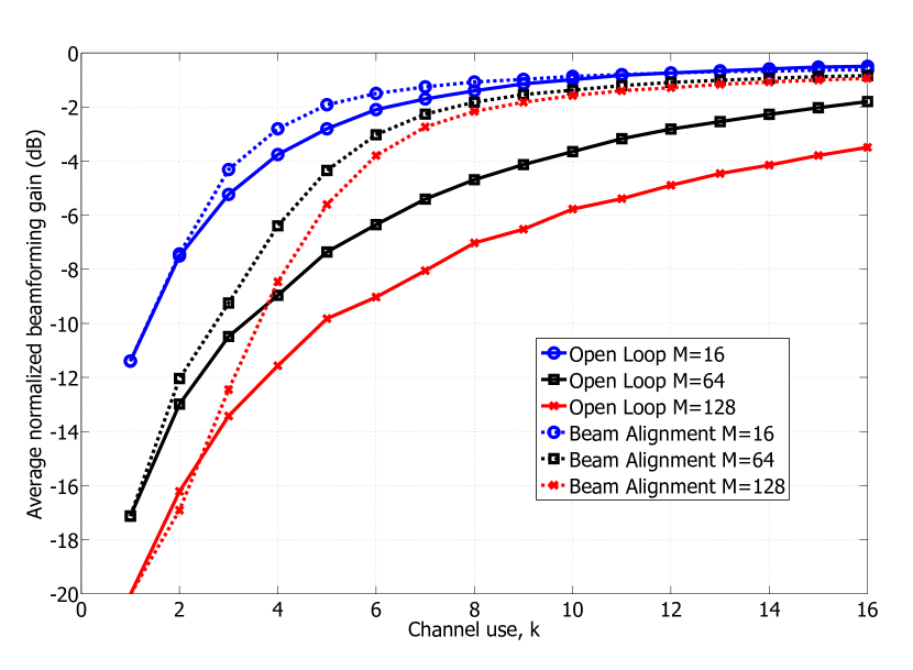
Figure 2: Average normalized beamforming gain $\lvert{\mathbf{h}}^{*}{\widehat{{\mathbf{h}}}}^{(k)}\rvert^{2}$ for a line-of-sight channel.

The closed-loop beam alignment algorithm is able to increase the average beamforming gain over orthogonal training for a small number of channel uses. At $k=5$, there is a $0.4$dB gain for $M=16$, a $3$dB gain for $M=64$, and a $5$dB gain for $M=128$. The beam alignment scheme gives considerable improvement for $K/M\ll 1$, and the improvement over open-loop grows with $M$.

V Conclusion

This work developed a closed-loop beam alignment scheme which, through the use of feedback after each channel use, sequentially designs sounding vectors to probe the channel in an efficent manner. This scheme provides a practical channel estimation algorithm for massive MIMO, where large scale arrays make optimal training impractical. A generalized maximum likelihood detector was developed to jointly perform the channel estimation and channel quantization. Since beamforming gain is only concerned with the direction of the channel, the detector replaces the channel gain by its maximum likelihood estimate. Sounding vectors are selected to minimize the misalignment cost function, a metric updated with knowledge of the previous receive samples in a Bayesian framework. The closed-loop beam alignment scheme shows improved beamforming gain over conventional orthogonal training signals, especially for the $K<M$. Additional analysis is required to determine the necessary amount of training as the number of transmit antennas increases.

Consider two Gaussian random variables, $X=\mu_{x}+q_{x}n$ and $Y=\mu_{y}+q_{y}n$. It should be mentioned that the expression $\text{Pr}(\lvert X\rvert^{2}>\lvert Y\rvert^{2})$ in Appendix B of [7] is not applicable when both $X$ and $Y$ are functions of the same scalar noise term $n\sim\mathcal{CN}(0,1)$, in which for a scalar noise term $n$, $E[\lvert X-\mu_{x}\rvert^{2}]E[\lvert Y-\mu_{y}\rvert^{2}]-\lvert E\left[(X-\mu_{x})(Y-\mu_{y})^{*}\right]\rvert^{2}=0$.

The inequality inside the probability expression, $\lvert\mu_{x}+q_{x}n\rvert^{2}>\lvert\mu_{y}+q_{y}n\rvert^{2}$, can be simplified by completing the square and rearranging terms for three separate cases (which depend on the magnitudes of $q_{x}$ and $q_{y}$),

$$\halign to=0.0pt{\relax\global\advance\@IEEEeqncolcnt by 1\relax\begingroup\csname @IEEEeqnarraycolPREr\endcsname#\relax\relax\relax\relax\relax\relax\relax\relax\relax\relax\csname @IEEEeqnarraycolPOSTr\endcsname\relax\relax\relax\relax\relax\relax\relax\relax\relax\relax\endgroup&\relax\global\advance\@IEEEeqncolcnt by 1\relax\begingroup\csname @IEEEeqnarraycolPREl\endcsname#\relax\relax\relax\relax\relax\relax\relax\relax\relax\relax\csname @IEEEeqnarraycolPOSTl\endcsname\relax\relax\relax\relax\relax\relax\relax\relax\relax\relax\endgroup&\global\advance\@IEEEeqncolcnt by 1\relax\bgroup#\egroup&\global\advance\@IEEEeqncolcnt by 1\relax\hbox to\z@\bgroup\hss#\egroup\cr$\displaystyle\text{Pr}\left( \lvert\mu_{x} + q_{x} n\rvert^{2} > \lvert\mu_{y} + q_{y} n\rvert^{2} \right) = $\hfil&{{}\vrule width=0.0pt,height=0.0pt,depth=0.0pt}&0.0pt{\hss}\cr\penalty 100\vskip 3.0pt\vskip 0.0pt\cr\hfil$\displaystyle\qquad\begin{cases}\text{Pr}\left( \lvert Z\rvert^{2} < \left|\frac{\mu_{x} q_{y} - q_{x} \mu_{y}}{\lvert q_{y}\rvert^{2} - \lvert q_{x}\rvert^{2}} \right|^{2} \right) &\text{ if } \lvert q_{y}\rvert^{2} > \lvert q_{x}\rvert^{2}\\ \text{Pr}\left( \lvert Z\rvert^{2} > \left|\frac{\mu_{x} q_{y} - q_{x} \mu_{y}}{\lvert q_{y}\rvert^{2} - \lvert q_{x}\rvert^{2}} \right|^{2} \right) &\text{ if } \lvert q_{y}\rvert^{2} < \lvert q_{x}\rvert^{2}\\ \text{Pr}\left( V < \frac{\lvert\mu_{y}\rvert^{2} - \lvert\mu_{x}\rvert^{2}}{2} \right) &\text{ if } \lvert q_{y}\rvert^{2} = \lvert q_{x}\rvert^{2}\\ \end{cases} $&$\displaystyle$\hfil&{\vrule width=0.0pt,height=0.0pt,depth=0.0pt}&0.0pt{\hss}\cr}$$

where $Z=n+\frac{\mu_{y}q_{y}^{*}-\mu_{x}q_{x}^{*}}{\lvert q_{y}\rvert^{2}-\lvert q_{x}\rvert^{2}}$ is a complex Gaussian random variable and $V=\text{Re}\{\mu_{y}^{*}q_{y}-\mu_{x}^{*}q_{x}\}\text{Re}\{n\}-\text{Im}\{\mu_{y}^{*}q_{y}-\mu_{x}^{*}q_{x}\}\text{Im}\{n\}$ is a real Gaussian random variable. $\lvert Z\rvert^{2}$ is a noncentral chi-squared random variable with $\text{Pr}(\lvert Z\rvert^{2}<z)=1-Q_{1}(\lvert\lambda\rvert,\sqrt{z})$ and $V$ is the sum of two independent real Gaussian random variables, with $\text{Pr}(V<v)=\frac{1}{2}\left(1+\text{erf}\left(v/\sqrt{2\lvert\mu_{y}^{*}q_{y}-\mu_{x}^{*}q_{x}\rvert^{2}}\right)\right)$. We then conclude the result in (1).

References

[1]
B. Hassibi and B. M. Hochwald, “How much training is needed in
multiple-antenna wireless links?” IEEE Trans. Inf. Theory, vol. 49,
no. 4, pp. 951–963, Apr. 2003.
[2]
J. Zhang, T. Yang, and Z. Chen, “Under-determined training and estimation for
distributed transmit beamforming systems,” IEEE Trans. Wireless
Commun., vol. 12, no. 4, pp. 1936–1946, Mar. 2013.
[3]
D. Fuhrmann, “Adaptive sensing of target signature with unknown amplitude,”
in 42nd Asilomar Conference, Oct. 2008, pp. 218–222.
[4]
D. J. Love, J. Choi, and P. Bidigare, “A closed-loop training approach for
massive MIMO beamforming systems,” in Conference on Information
Sciences and Systems, Mar. 2013, pp. 1–5.
[5]
S. Hur, T. Kim, D. J. Love, J. V. Krogmeier, T. A. Thomas, and A. Ghosh,
“Millimeter wave beamforming for wireless backhaul and access in small cell
networks,” IEEE Tran. Commun., vol. 61, no. 10, pp. 4391–4403, Oct.
2013.
[6]
F. Rusek, D. Persson, B. K. Lau, E. Larsson, T. Marzetta, O. Edfors, and
F. Tufvesson, “Scaling up MIMO: Opportunities and challenges with very
large arrays,” IEEE Signal Process. Mag., vol. 30, no. 1, pp. 40–60,
2013.
[7]
J. G. Proakis, Digital Communications, 4th ed. McGraw-Hill, 2001.