$H^{\infty}$ Design of Periodically Nonuniform Interpolation and Decimation for Non-Band-Limited Signals

Masaaki Nagahara ,ย  Masaki Ogura ย andย  Yutaka Yamamoto M. Nagahara and Y. Yamamoto are with Graduate School of Informatics, Kyoto University. M. Ogura is with Department of Mathematics and Statistics, Texas Tech University. The corresponding author is M. Nagahara (nagahara@ieee.org).
Abstract.

In this paper, we consider signal interpolation of discrete-time signals which are decimated nonuniformly. A conventional interpolation method is based on the sampling theorem, and the resulting system consists of an ideal filter with complex-valued coefficients. While the conventional method assumes band limitation of signals, we propose a new method by sampled-data $H^{\infty}$ optimization. By this method, we can remove the band-limiting assumption and the optimal filter can be with real-valued coefficients. Moreover, we show that without band-limited assumption, there can be the optimal decimation patterns among ones with the same ratio. By examples, we show the effectiveness of our method.

1. Introduction

Interpolation is a fundamental operation in digital signal processing, and has many applications such as signal reconstruction, signal compression/expansion, and resizing/rotating digital images [13, 2]. If digital data (discrete-time signals) to be interpolated are spaced uniformly on the time axis, the uniform interpolation is executed by an expander and a digital filter (called an interpolation filter) [13], which is conventionally designed via the sampling theorem.

Periodically nonuniform interpolation (or decimation) also plays an important role in signal processing, such as signal compression by nonuniform filterbanks [8], super-resolution image processing [9], and time-interleaved AD converters [10]. The design has been studied by many researchers [14, 8, 15, 3, 4], in which the design methods are based on the generalized sampling theorem, assuming that the original signals to be sampled are band-limited below the Nyquist frequency. Then the optimal filter (or the perfect reconstruction filter) is given by an ideal lowpass filter with complex coefficients [14, 13]. Since the ideal filter cannot be realized, approximation methods are also proposed; see in particular [14, 15].

On the other hand, real signals such as audio signals (esp.ย orchestral music) violate the band-limiting assumption in the sampling theorem, that is, they have some frequency components beyond the Nyquist frequency. In view of this, we have to take account of the whole frequency range in designing interpolation systems. For this purpose, sampled-data $H^{\infty}$ optimization [1, 6] is very adequate.

A similar philosophy has also been presented and proposed by Unser and co-workers [12, 11]. This method is a generalization of Shannon sampling theory intending to give a machinery that works for signals that are not necessarily perfectly band-limited. The method works well for those analog signals that belong to a prespecified subspace, but not necessarily so for those that do not. It is even shown that their method can lead to an unstable reconstruction filter [7]. Moreover, the signal subspace is constructed by the linear span of a given generating function, but it is not easy to identify the generating function in real applications. On the other hand, our approach models the signal subspace in terms of analog (continuous-time) frequency characteristics, which can easily be identified by modeling a signal generator by physical laws or through the Fourier transform of real signals.

The main objective of this paper is to propose a new design method for nonuniform interpolation via sampled-data Hโˆžsuperscript๐ปH^{\infty} optimization. This design problem is formulated by minimizing the Hโˆžsuperscript๐ปH^{\infty} norm (L2superscript๐ฟ2L^{2}-induced norm) of the error system between the delayed original analog signals and the output of the reconstruction system. Since this error system includes both continuous- and discrete-time signals (systems), the optimization is an infinite dimensional one. To convert this to a finite dimensional optimization, we introduce the fast discretization method [1, Chap.ย 8],ย [18]. By this method, the optimal interpolation filter can be obtained by numerical computations. MATLAB codes for this optimization are available through [20].

We also show in this paper that there are cases with the same decimation rates but the optimal reconstruction performances can differ when the decimation patterns are different. That is, the performance depends on the decimation pattern. Note that this property cannot be captured via the sampling theorem.

The paper is organized as follows. We first define nonuniform decimation with a decimation pattern in Section 2. We show that this definition includes the block decimation introduced in [8]. In Section 3 we define nonuniform expanders and formulate the interpolation problem using such an expander for non-band-limited signals. A design procedure and implementation as a multirate filterbank are also given in this section. In Section 4, we consider optimal decimation pattern analysis. Section 5 shows design examples. In this section, we will show a result of our optimization and compare it with a conventional design proposed in [14, 13]. Here we will show our method is superior to the conventional method. Optimal decimation patterns for several decimation ratios are also presented. Section 6 concludes our result.

Notation

Throughout this paper, we use the following notation:

${\mathbb{R}}$, ${\mathbb{R}}^{M},{\mathbb{R}}^{M\times N}$:

the sets of real numbers, real valued column vectors of size $M$, and $M$ by $N$ real valued matrices, respectively.

$L^{2}$:

the Lebesgue space consisting of all square integrable real functions.

$z$:

the symbol for $Z$ transform (the $Z$ transform of the forward shift operator).

s๐‘ s:

the symbol for Laplace transform (the Laplace transform of the differentiator $\frac{{\mathrm{d}}}{{\mathrm{d}}t}$).

$A^{\top}$:

the transpose of a matrix $A$.

$I_{N}$:

the $N\times N$ identity matrix.

๐›๐ฅ๐จ๐œ๐ค๐๐ข๐š๐ โ€‹(A,B,โ€ฆ,C)๐›๐ฅ๐จ๐œ๐ค๐๐ข๐š๐ ๐ด๐ตโ€ฆ๐ถ\mathbf{blockdiag}(A,B,\ldots,C):

a block-diagonal matrix of matrices $A$, $B$, $\ldots$, $C$, that is,

๐›๐ฅ๐จ๐œ๐ค๐๐ข๐š๐ โ€‹(A,B,โ€ฆ,C)=[ABโ‹ฑC].๐›๐ฅ๐จ๐œ๐ค๐๐ข๐š๐ ๐ด๐ตโ€ฆ๐ถdelimited-[]๐ดmissing-subexpressionmissing-subexpressionmissing-subexpressionmissing-subexpression๐ตmissing-subexpressionmissing-subexpressionmissing-subexpressionmissing-subexpressionโ‹ฑmissing-subexpressionmissing-subexpressionmissing-subexpressionmissing-subexpression๐ถ\mathbf{blockdiag}(A,B,\ldots,C)=\left[\begin{array}[]{cccc}A&&&\\ &B&&\\ &&\ddots&\\ &&&C\end{array}\right].
$\left[\begin{array}[]{c|c}A&B\\ \hline\cr C&D\end{array}\right]$:

a state-space representation for a continuous-time system Cโ€‹(sโ€‹Iโˆ’A)โˆ’1โ€‹B+D๐ถsuperscript๐‘ ๐ผ๐ด1๐ต๐ทC(sI-A)^{-1}B+D or discrete-time one $C(zI-A)^{-1}B+D$.

2. Nonuniform Decimation and Decimation Patterns

Let us consider the discrete-time signal $x:=\{x_{0},x_{1},x_{2},\ldots\}.$ Then nonuniform decimation by ${\mathbf{M}}:=[1,1,0]$ (we call this a decimation pattern) is defined by

$$(\downarrow\!{\mathbf{M}})x:=\{x_{0},x_{1},x_{3},x_{4},x_{6},\ldots\}.$$ (1)

That is, we first divide the time axis into segments of length three (the number of the elements in ${\mathbf{M}}$), then, in each segment, retain the samples corresponding to 1 in ${\mathbf{M}}$ and discard the samples corresponding to 0. We then define a general nonuniform decimation with decimation pattern

$${\mathbf{M}}:=\left[\begin{array}[]{cccc}b_{0}&b_{1}&\ldots&b_{M-1}\end{array}\right],\quad b_{i}\in\{0,1\},$$ (2)

where $M$ is the number of elements in ${\mathbf{M}}$. Let $i_{1},i_{2},\ldots,i_{N}$ satisfying

$$0\leq i_{1}<i_{2}<\ldots<i_{N}\leq M-1$$

be the indices of $b_{i}$โ€™s such that $b_{i_{1}}=\cdots=b_{i_{N}}=1$ where $N$ is the number of ones in ${\mathbf{M}}$. Then for $x=\{x_{0},x_{1},\ldots\}$, the nonuniform decimation is defined by

$$(\downarrow\!{\mathbf{M}})x=\left\{x_{i_{1}},x_{i_{2}},\ldots,x_{i_{N}},x_{M+i_{1}},x_{M+i_{2}},\ldots\right\}.$$

This definition includes the so-called block decimation [8], in which the first $R_{1}$ samples of each segment of $R_{2}$ samples are retained while the rest are discarded. By our notation, the block decimation $R_{2}:R_{1}$ is represented as $\downarrow\!{\mathbf{M}}$ with

$${\mathbf{M}}={[\underbrace{1,\ldots,1}_{R_{1}},\underbrace{0,\ldots,0}_{R_{2}-R_{1}}]}.$$

The decimation ratio of ${\mathbf{M}}$ is defined to be $M/N$. Note that since $N\leq M$, the ratio is always greater than or equal to 1. By our definition, the uniform decimator $\downarrow\!M$ where $M$ is a positive integer is represented as a special case of nonuniform decimator

$$\downarrow\!M=\downarrow\!{\mathbf{M}},\quad{\mathbf{M}}=[1,\underbrace{0,0,\ldots,0}_{M-1}],$$

with decimation ratio $M$.

3. Design of Interpolation Filter

3.1. Nonuniform Interpolation

To consider signal reconstruction from a nonuniformly decimated signal $(\downarrow\!{\mathbf{M}})x$, we define the nonuniform expander $\uparrow\!{\mathbf{M}}$. Let ${\mathbf{M}}=[1,1,0]$. Then we define $(\uparrow\!{\mathbf{M}})x$ for $x=\{x_{0},x_{1},\ldots\}$ by

$$(\uparrow\!{\mathbf{M}})x:=\{x_{0},x_{1},0,x_{2},x_{3},0,x_{4},\ldots\}.$$

That is, we first divide the time axis into segments of length two (the number of 1โ€™s in ${\mathbf{M}}$), then insert 0โ€™s into the position corresponding to 0โ€™s in ${\mathbf{M}}$. By this definition, the uniform expander $\uparrow\!M$ where $M$ is a positive integer is represented as a nonuniform expander

$$\uparrow\!M=\uparrow\!{\mathbf{M}},\quad{\mathbf{M}}=[1,\underbrace{0,0,\ldots,0}_{M-1}].$$

Applying this to the decimated sequence (1), we have

$$v:=(\uparrow\!{\mathbf{M}})(\downarrow\!{\mathbf{M}})x=\{x_{0},x_{1},0,x_{3},x_{4},0,x_{6},\ldots\}.$$

The procedure is shown in Fig.ย 1.

1101101101101
Figure 1. Nonuniform decimation and expansion (${\mathbf{M}}=[1,1,0]$): original sequence $x$ (above) and $(\uparrow\!{\mathbf{M}})(\downarrow\!{\mathbf{M}})x$ (below).

In general case of the decimation pattern (2), the expansion is given by

$$\begin{split}v&=(\uparrow\!{\mathbf{M}})(\downarrow\!{\mathbf{M}})x\\ &=\{b_{0}x_{0},b_{1}x_{1},\ldots,b_{M-1}x_{M-1},b_{0}x_{M},b_{1}x_{M+1},\ldots\}.\end{split}$$

3.2. Polyphase Representation

The interpolation of a decimated signal is completed by filtering $v=(\uparrow\!{\mathbf{M}})(\downarrow\!{\mathbf{M}})x$ by a digital filter ${\mathcal{K}}$ (see Fig.ย 2 (a)).

$\downarrow\!{\mathbf{M}}$ $\uparrow\!{\mathbf{M}}$ ${\mathcal{K}}$ $x$ $y$ $v$(a)${\mathbf{L}}_{M}$ $E$ $\widetilde{{\mathcal{K}}}$ ${\mathbf{L}}_{M}^{-1}$ $x$ $y$(b)
Figure 2. (a) Nonuniform decimation and interpolation, (b) polyphase representation of (a).

The decimation and interpolation process ${\mathcal{K}}(\uparrow\!{\mathbf{M}})(\downarrow\!{\mathbf{M}})$ is periodically time-varying. To convert this equivalently to a linear time-invariant system, we introduce the polyphase decomposition [13]. Let ${\mathbf{L}}_{M}$ be the polyphase decomposition operator, that is,

$${\mathbf{L}}_{M}:\left\{x_{0},x_{1},\ldots\right\}\mapsto\left\{\left[\begin{array}[]{c}x_{0}\\ x_{1}\\ \vdots\\ x_{M-1}\end{array}\right],\left[\begin{array}[]{c}x_{M}\\ x_{M+1}\\ \vdots\\ x_{2M-1}\end{array}\right],\ldots\right\}.$$

By this operator, the nonuniform decimator $\downarrow\!{\mathbf{M}}$ and expander $\uparrow\!{\mathbf{M}}$ can be represented as filterbanks.

Lemma 1.

The following two equalities hold:

  1. (1)

    $\downarrow\!{\mathbf{M}}={\mathbf{L}}_{N}^{-1}E{\mathbf{L}}_{M},$

  2. (2)

    $\uparrow\!{\mathbf{M}}={\mathbf{L}}_{M}^{-1}E^{\top}{\mathbf{L}}_{N},$

where $E=[E_{ij}]$ is an $N\times M$ matrix whose elements are defined as follows:

$$E_{ij}=\begin{cases}1,\quad(i,j)=(1,i_{1}+1),(2,i_{2}+1),\ldots,(N,i_{N}+1),\\ 0,\quad\text{otherwise}.\end{cases}$$

Proof.

  1. (1)

    For $v=[v_{0},v_{1},\ldots,v_{M-1}]^{\top}\in{\mathbb{R}}^{M}$ we have

    $$Ev=[v_{i_{1}},v_{i_{2}},\ldots,v_{i_{N}}]^{\top}\in{\mathbb{R}}^{N}.$$

    By using this, for any sequence $x=\{x_{0},x_{1},x_{2},\ldots,\}$ we have

    $$\begin{split}E{\mathbf{L}}_{M}x&=E\left\{\begin{bmatrix}x_{0}\\ x_{1}\\ \vdots\\ x_{M-1}\end{bmatrix},~{}\begin{bmatrix}x_{M}\\ x_{M+1}\\ \vdots\\ x_{2M-1}\end{bmatrix},\ldots\right\}\\ &=\left\{E\begin{bmatrix}x_{0}\\ x_{1}\\ \vdots\\ x_{M-1}\end{bmatrix},~{}E\begin{bmatrix}x_{M}\\ x_{M+1}\\ \vdots\\ x_{2M-1}\end{bmatrix},\ldots\right\}\\ &=\left\{\begin{bmatrix}x_{i_{1}}\\ x_{i_{2}}\\ \vdots\\ x_{i_{N}}\end{bmatrix},~{}\begin{bmatrix}x_{M+i_{1}}\\ x_{M+i_{2}}\\ \vdots\\ x_{M+i_{N}}\end{bmatrix},\ldots\right\}.\end{split}$$

    Therefore, for any $x$ we have

    $$\begin{split}{\mathbf{L}}_{N}^{-1}E{\mathbf{L}}_{M}x&=\left\{x_{i_{1}},x_{i_{2}},\ldots,x_{i_{N}},x_{M+i_{1}},x_{M+i_{2}},\ldots,x_{M+i_{N}},\ldots\right\}\\ &=(\downarrow\!{\mathbf{M}})x.\end{split}$$

    That is, ${\mathbf{L}}_{N}^{-1}E{\mathbf{L}}_{M}=\downarrow\!{\mathbf{M}}$.

  2. (2)

    The matrix $E$ can be represented by

    $$E^{\top}=[e_{i_{1}},e_{i_{2}},\ldots,e_{i_{N}}],$$

    where

    $$e_{i}=[0,\ldots,0,\stackrel{{\scriptstyle i+1}}{{\stackrel{{\scriptstyle\vee}}{{1}}}},0,\ldots,0]^{\top}\in{\mathbb{R}}^{M},i=0,1,\ldots,M-1.$$

    By using this, for any vector of

    $$w=[w_{0},w_{1},\ldots,w_{N-1}]^{\top}\in{\mathbb{R}}^{N},$$

    we have

    EโŠคโ€‹w=[ei1,ei2,โ€ฆ,eiN]โ€‹[w0w1โ‹ฎwNโˆ’1]=ei1โ€‹w0+ei2โ€‹w1+โ‹ฏ+eiNโ€‹wNโˆ’1=[0,โ€ฆ,0,w0โˆจ0i1+10,0,โ€ฆ,0,w1โˆจ1i2+11,0,โ€ฆ,0,wNโˆ’1โˆจNโˆ’1iN+1Nโˆ’1,0,โ€ฆ,0]โŠคโˆˆโ„M.superscript๐ธtop๐‘คsubscript๐‘’subscript๐‘–1subscript๐‘’subscript๐‘–2โ€ฆsubscript๐‘’subscript๐‘–๐‘matrixsubscript๐‘ค0subscript๐‘ค1โ‹ฎsubscript๐‘ค๐‘1subscript๐‘’subscript๐‘–1subscript๐‘ค0subscript๐‘’subscript๐‘–2subscript๐‘ค1โ‹ฏsubscript๐‘’subscript๐‘–๐‘subscript๐‘ค๐‘1superscript0โ€ฆ0superscriptsuperscriptsubscript๐‘ค0subscript๐‘–110โ€ฆ0superscriptsuperscriptsubscript๐‘ค1subscript๐‘–210โ€ฆ0superscriptsuperscriptsubscript๐‘ค๐‘1subscript๐‘–๐‘10โ€ฆ0topsuperscriptโ„๐‘€\begin{split}E^{\top}w&=[e_{i_{1}},e_{i_{2}},\ldots,e_{i_{N}}]\begin{bmatrix}w_{0}\\ w_{1}\\ \vdots\\ w_{N-1}\end{bmatrix}\\ &=e_{i_{1}}w_{0}+e_{i_{2}}w_{1}+\cdots+e_{i_{N}}w_{N-1}\\ &=[0,\ldots,0,\stackrel{{\scriptstyle i_{1}+1}}{{\stackrel{{\scriptstyle\vee}}{{w_{0}}}}},0,\ldots,0,\stackrel{{\scriptstyle i_{2}+1}}{{\stackrel{{\scriptstyle\vee}}{{w_{1}}}}},0,\ldots,0,\stackrel{{\scriptstyle i_{N}+1}}{{\stackrel{{\scriptstyle\vee}}{{w_{N-1}}}}},0,\ldots,0]^{\top}\in{\mathbb{R}}^{M}.\end{split}

    By this property and the same computation as in the proof of $\downarrow\!{\mathbf{M}}$, the equality ${\mathbf{L}}_{M}^{-1}E^{\top}{\mathbf{L}}_{N}=\uparrow\!{\mathbf{M}}$ can be proved.

$\Box$

For example, if ${\mathbf{M}}=[1,1,0]$ ($M=3$, $N=2$, $i_{1}=1$, $i_{2}=2$) then $\uparrow\!{\mathbf{M}}$ and $\downarrow\!{\mathbf{M}}$ are represented as filterbanks shown in Fig.3.

$+$ $\downarrow\!3$ $\uparrow\!2$ $\uparrow\!2$ $\downarrow\!3$ $z$ $z^{-1}$ $+$ $\downarrow\!2$ $\uparrow\!3$ $\uparrow\!3$ $\downarrow\!2$ $z$ $z^{-1}$(a)(b)$E{\mathbf{L}}_{3}$ ${\mathbf{L}}_{3}^{-1}E^{\top}$ ${\mathbf{L}}_{2}^{-1}$ ${\mathbf{L}}_{2}$
Figure 3. Filterbank representation of (a) $\downarrow\!{\mathbf{M}}$ and (b) $\uparrow\!{\mathbf{M}}$ with ${\mathbf{M}}=[1,1,0]$ ($M=3$, $N=2$).

In this case, the matrix $E$ is given by

$$E=\left[\begin{array}[]{ccc}1&0&0\\ 0&1&0\end{array}\right].$$

By Lemma 1, we can represent the decimation and interpolation process ${\mathcal{K}}(\uparrow\!{\mathbf{M}})(\downarrow\!{\mathbf{M}})$ by a polyphase decomposition. In fact, we have the following theorem (see also Fig.ย 2).

Theorem 1.

The following identity holds:

$${\mathcal{K}}(\uparrow\!{\mathbf{M}})(\downarrow\!{\mathbf{M}})={\mathbf{L}}_{M}^{-1}\widetilde{{\mathcal{K}}}E{\mathbf{L}}_{M},$$ (3)

where

$$\widetilde{{\mathcal{K}}}:={\mathbf{L}}_{M}{\mathcal{K}}{\mathbf{L}}_{M}^{-1}E^{\top}.$$ (4)

Proof.

By Lemma 1 and the identities ${\mathbf{L}}_{M}^{-1}{\mathbf{L}}_{M}=1$ and ${\mathbf{L}}_{N}{\mathbf{L}}_{N}^{-1}=I_{N}$ ($I_{N}$ is the $N\times N$ identity matrix), we have

$$\begin{split}{\mathcal{K}}(\uparrow\!{\mathbf{M}})(\downarrow\!{\mathbf{M}})&={\mathbf{L}}_{M}^{-1}{\mathbf{L}}_{M}{\mathcal{K}}\left({\mathbf{L}}_{M}^{-1}E^{\top}{\mathbf{L}}_{N}\right)\left({\mathbf{L}}_{N}^{-1}E{\mathbf{L}}_{M}\right)\\ &={\mathbf{L}}_{M}^{-1}\left({\mathbf{L}}_{M}{\mathcal{K}}{\mathbf{L}}_{M}^{-1}E^{\top}\right)E{\mathbf{L}}_{M}\\ &={\mathbf{L}}_{M}^{-1}\widetilde{{\mathcal{K}}}E{\mathbf{L}}_{M}.\end{split}$$

$\Box$

By this theorem, we can easily see that $\widetilde{{\mathcal{K}}}$ is a linear time-invariant system with $M$ inputs and $M$ outputs [1, Chap. 8], and ${\mathcal{K}}(\uparrow\!{\mathbf{M}})(\downarrow\!{\mathbf{M}})$ is $M$-periodic [5].

3.3. $H^{\infty}$ Optimal Interpolation for Non-Band-Limited Signals

We now consider the signal space to which the original continuous-time signals before sampling and decimation belong. Let $h$ denote the sampling period. The nonuniform sampling theory [14, 13] assumes this space as the band-limited subspace defined by

$$BL:=\left\{u\in L^{2}:\mathrm{supp}~{}\hat{u}\subset\Omega(M/N)\right\},$$

where $\hat{u}$ is the Fourier transform of $u\in L^{2}$, and

$$\Omega(M/N):=\left(-\frac{N\pi}{Mh},\frac{N\pi}{Mh}\right).$$

On the other hand, we consider another subspace of $L^{2}$ which includes non-band-limited signals, defined by

$${FL^{2}}:=\left\{u\in L^{2}:u=Fw,~{}w\in L^{2}\right\},$$

where $F$ is a stable linear time-invariant continuous-time system whose transfer function is finite-dimensional and strictly proper. This space is a model for the signal subspace to which the input analog signals belong. A merit for this model is that one can naturally and easily include the analog frequency characteristic in the model via physical laws or executing Fourier transform of real signals. This is an advantage over the generalized sampling theory [12, 11], in which the signal subspace is modeled by the linear span of a given generating function.

Moreover, this subspace ${FL^{2}}$ is essentially wider than $BL$. In fact, the following lemma holds:

Lemma 2.

Assume that $F({\mathrm{j}}\omega)$ has no zeros in $\Omega(M/N)$. Then $BL\subset{FL^{2}}$.

Proof.

Let $u\in BL$. Define a function $w$ such that

$$\hat{w}({\mathrm{j}}\omega)=\begin{cases}\hat{F}({\mathrm{j}}\omega)^{-1}\hat{u}({\mathrm{j}}\omega),&\quad\text{if}~{}\omega\in\Omega(M/N),\\ 0,&\quad\text{if}~{}\omega\notin\Omega(M/N).\end{cases}$$

Since $u\in BL$, $\hat{u}({\mathrm{j}}\omega)=0$ if $\omega\notin\Omega(M/N)$, and hence we have $\hat{u}({\mathrm{j}}\omega)=\hat{F}({\mathrm{j}}\omega)\hat{w}({\mathrm{j}}\omega)$ for all $\omega\in{\mathbb{R}}$, or $u=Fw$. Then we show that $w\in L^{2}$. In fact, we have

$$\begin{split}\|w\|_{2}^{2}&=\int_{0}^{\infty}|w(t)|^{2}{\mathrm{d}}t\\ &=\frac{1}{2\pi}\int_{{\mathbb{R}}}|\hat{w}({\mathrm{j}}\omega)|^{2}{\mathrm{d}}\omega\\ &=\frac{1}{2\pi}\int_{\Omega(M/N)}|\hat{F}({\mathrm{j}}\omega)^{-1}u({\mathrm{j}}\omega)|^{2}{\mathrm{d}}\omega\\ &\leq\frac{1}{2\pi}~{}\|u\|_{2}^{2}~{}\left(\max_{\omega\in\Omega(M/N)}\left|\hat{F}({\mathrm{j}}\omega)^{-1}\right|\right)^{2}\\ &=\frac{1}{2\pi}~{}\|u\|_{2}^{2}~{}\left(\min_{\omega\in\Omega(M/N)}\left|\hat{F}({\mathrm{j}}\omega)\right|^{2}\right)^{-1}\\ &<\infty.\end{split}$$

Therefore, we have $u\in{FL^{2}}$. $\Box$

To consider signal reconstruction for non-band-limited signals in ${FL^{2}}$, let us consider the error system shown in Fig.ย 4. In this figure, $F$ is a linear system defining the signal space ${FL^{2}}$. The block ${\mathcal{S}}_{h}$ represents the ideal sampler with sampling period $h$, and ${\mathcal{H}}_{h}$ the zero-order hold with the same sampling period. The delay eโˆ’Lโ€‹ssuperscript๐‘’๐ฟ๐‘ e^{-Ls} is a reconstruction delay.

$F$ ${\mathcal{S}}_{h}$ ${\mathbf{L}}_{M}$ $E$ $\widetilde{{\mathcal{K}}}$ ${\mathbf{L}}_{M}^{-1}$ ${\mathcal{H}}_{h}$eโˆ’Lโ€‹ssuperscript๐‘’๐ฟ๐‘ e^{-Ls}$w$ $u$ $e$ $-$
Figure 4. Error system $T_{ew}(\widetilde{{\mathcal{K}}},{\mathbf{M}})$.

Then our optimization problem is formulated as a sampled-data $H^{\infty}$ optimization. Let $T_{ew}(\widetilde{{\mathcal{K}}},{\mathbf{M}})$ be the error system from the continuous-time signal $w$ to the error $e$ (see Fig.ย 4).

Problem 1.

Given a decimation pattern ${\mathbf{M}}$, find the optimal filter $\widetilde{{\mathcal{K}}}$ that minimizes

Jโ€‹(๐’ฆ~):=โ€–Teโ€‹wโ€‹(๐’ฆ~,๐Œ)โ€–โˆž=supwโˆˆL2wโ‰ 0โ€–Teโ€‹wโ€‹(๐’ฆ~,๐Œ)โ€‹wโ€–2โ€–wโ€–2.assign๐ฝ~๐’ฆsubscriptnormsubscript๐‘‡๐‘’๐‘ค~๐’ฆ๐Œsubscriptsupremum๐‘คsuperscript๐ฟ2๐‘ค0subscriptnormsubscript๐‘‡๐‘’๐‘ค~๐’ฆ๐Œ๐‘ค2subscriptnorm๐‘ค2J(\widetilde{{\mathcal{K}}}):=\|T_{ew}(\widetilde{{\mathcal{K}}},{\mathbf{M}})\|_{\infty}=\sup_{\begin{subarray}{c}w\in L^{2}\\ w\neq 0\end{subarray}}\frac{\|T_{ew}(\widetilde{{\mathcal{K}}},{\mathbf{M}})w\|_{2}}{\|w\|_{2}}. (5)

3.4. Computation of Optimal Filter

To solve Problem 1, the $H^{\infty}$ norm $\|T_{ew}(\widetilde{{\mathcal{K}}},{\mathbf{M}})\|_{\infty}$ has to be evaluated. By using the fast discretization method, we can approximately obtain the optimal $\widetilde{{\mathcal{K}}}$ with arbitrary precision.

First we introduce useful properties [1] for computing the optimal filter.

Lemma 3.

Let $\tau$ be a positive real number, and $P_{c}$ a continuous-time linear time-invariant system. Then ${\mathcal{D}}_{\tau}\left(P_{c}\right):={\mathcal{S}}_{\tau}P_{c}{\mathcal{H}}_{\tau}$ is a discrete-time linear time-invariant system. The state space realization is given by

$${\mathcal{D}}_{\tau}\left(\left[\begin{array}[]{c|c}A&B\\ \hline\cr C&D\end{array}\right]\right)=\left[\begin{array}[]{c|c}e^{A\tau}&\int_{0}^{\tau}e^{At}B{\mathrm{d}}t\\ \hline\cr C&D\end{array}\right].$$ (6)
Lemma 4.

Let $n$ be a positive integer and $P$ a discrete-time linear time-invariant system. Then ${\mathcal{L}}_{n}\left(P\right):={\mathbf{L}}_{n}P{\mathbf{L}}_{n}^{-1}$ is also a discrete-time linear time-invariant system. The state space realization is given by

$${\mathcal{L}}_{n}\left(\left[\begin{array}[]{c|c}A&B\\ \hline\cr C&D\end{array}\right]\right)=\left[\begin{array}[]{c|cccc}A^{n}&A^{n-1}B&A^{n-2}B&\ldots&B\\ \hline\cr C&D&0&\ldots&0\\ CA&CB&D&\ldots&0\\ \vdots&\vdots&\ddots&\vdots\\ CA^{n-1}&CA^{n-2}B&CA^{n-3}B&\ldots&D\end{array}\right].$$ (7)

In particular, for a scalar $d\in{\mathbb{R}}$ and a matrix $D\in{\mathbb{R}}^{p\times q}$ we have respectively

โ„’nโ€‹(d)=dโ‹…In,โ„’nโ€‹(D)=๐›๐ฅ๐จ๐œ๐ค๐๐ข๐š๐ โ€‹(D,โ€ฆ,DโŸn).formulae-sequencesubscriptโ„’๐‘›๐‘‘โ‹…๐‘‘subscript๐ผ๐‘›subscriptโ„’๐‘›๐ท๐›๐ฅ๐จ๐œ๐ค๐๐ข๐š๐ subscriptโŸ๐ทโ€ฆ๐ท๐‘›{\mathcal{L}}_{n}\left(d\right)=d\cdot I_{n},\quad{\mathcal{L}}_{n}\left(D\right)=\mathbf{blockdiag}(\underbrace{D,\ldots,D}_{n}). (8)

Using these lemmas, we can obtain a discrete-time, linear and time-invariant system whose $H^{\infty}$ norm approximates $\|T_{ew}(\widetilde{{\mathcal{K}}},{\mathbf{M}})\|_{\infty}$ with arbitrary precision.

Theorem 2.

Assume that $L=mh$, where $m$ is a non-negative integer. Then there exists a sequence of linear time-invariant discrete-time systems {$T_{n}(\widetilde{{\mathcal{K}}},{\mathbf{M}})\}$ such that

$$\lim_{n\rightarrow\infty}\|T_{n}(\widetilde{{\mathcal{K}}},{\mathbf{M}})\|_{\infty}=\|T_{ew}(\widetilde{{\mathcal{K}}},{\mathbf{M}})\|_{\infty}.$$ (9)
$w_{n}$ $w$ $e$ $e_{n}$ ${\mathcal{S}}_{h/n}$ ${\mathcal{H}}_{h/n}$ $T_{ew}(\widetilde{{\mathcal{K}}})$
Figure 5. Fast discretization for $T_{ew}(\widetilde{{\mathcal{K}}},{\mathbf{M}})$.
$\begin{bmatrix}G_{11}&G_{12}\\ G_{21}&0\end{bmatrix}$ $\widetilde{{\mathcal{K}}}$
Figure 6. Block diagram for discrete-time $H^{\infty}$ optimization.

Proof.

We first approximate continuous-time signals $w$ and $e$ (see Fig.ย 4) to discrete-time ones via a fast sampler ${\mathcal{S}}_{h/n}$ and a fast hold ${\mathcal{H}}_{h/n}$ (see Fig.ย 5). Let $G_{n}$ be the system from $w_{n}$ to $e_{n}$ shown in Fig.ย 5. Then we have

Gn=๐’ฎh/nโ€‹Teโ€‹wโ€‹(๐’ฆ~,๐Œ)โ€‹โ„‹h/n=๐’ฎh/nโ€‹{eโˆ’mโ€‹hโ€‹sโˆ’โ„‹hโ€‹๐‹Mโˆ’1โ€‹๐’ฆ~โ€‹Eโ€‹๐‹Mโ€‹๐’ฎh}โ€‹Fโ€‹โ„‹h/n=zโˆ’mโ€‹nโ€‹๐’ฎh/nโ€‹Fโ€‹โ„‹h/nโˆ’๐’ฎh/nโ€‹โ„‹hโ€‹๐‹Mโˆ’1โ€‹๐’ฆ~โ€‹Eโ€‹๐‹Mโ€‹๐’ฎhโ€‹Fโ€‹โ„‹h/n.subscript๐บ๐‘›subscript๐’ฎโ„Ž๐‘›subscript๐‘‡๐‘’๐‘ค~๐’ฆ๐Œsubscriptโ„‹โ„Ž๐‘›subscript๐’ฎโ„Ž๐‘›superscript๐‘’๐‘šโ„Ž๐‘ subscriptโ„‹โ„Žsuperscriptsubscript๐‹๐‘€1~๐’ฆ๐ธsubscript๐‹๐‘€subscript๐’ฎโ„Ž๐นsubscriptโ„‹โ„Ž๐‘›superscript๐‘ง๐‘š๐‘›subscript๐’ฎโ„Ž๐‘›๐นsubscriptโ„‹โ„Ž๐‘›subscript๐’ฎโ„Ž๐‘›subscriptโ„‹โ„Žsuperscriptsubscript๐‹๐‘€1~๐’ฆ๐ธsubscript๐‹๐‘€subscript๐’ฎโ„Ž๐นsubscriptโ„‹โ„Ž๐‘›\begin{split}G_{n}&={\mathcal{S}}_{h/n}T_{ew}(\widetilde{{\mathcal{K}}},{\mathbf{M}}){\mathcal{H}}_{h/n}\\ &={\mathcal{S}}_{h/n}\left\{e^{-mhs}-{\mathcal{H}}_{h}{\mathbf{L}}_{M}^{-1}\widetilde{{\mathcal{K}}}E{\mathbf{L}}_{M}{\mathcal{S}}_{h}\right\}F{\mathcal{H}}_{h/n}\\ &=z^{-mn}{\mathcal{S}}_{h/n}F{\mathcal{H}}_{h/n}-{\mathcal{S}}_{h/n}{\mathcal{H}}_{h}{\mathbf{L}}_{M}^{-1}\widetilde{{\mathcal{K}}}E{\mathbf{L}}_{M}{\mathcal{S}}_{h}F{\mathcal{H}}_{h/n}.\end{split}

Now apply the operators ${\mathbf{L}}_{n}$ and ${\mathbf{L}}_{n}^{-1}$ to $G_{n}$. Using the identities [1, Chap.ย 8]

$${\mathcal{H}}_{h}={\mathcal{H}}_{h/n}{\mathbf{L}}_{n}^{-1}H,\quad{\mathcal{S}}_{h}=S{\mathbf{L}}_{n}{\mathcal{S}}_{h/n},$$

where

$$H:=[\underbrace{1,1,\ldots,1}_{n}]^{\top},\quad S:=[1,\underbrace{0,\ldots,0}_{n-1}],$$

we obtain

$$\begin{split}{\mathbf{L}}_{n}G_{n}{\mathbf{L}}_{n}^{-1}&={\mathbf{L}}_{n}z^{-mn}{\mathcal{S}}_{h/n}F{\mathcal{H}}_{h/n}{\mathbf{L}}_{n}^{-1}-{\mathbf{L}}_{n}{\mathcal{S}}_{h/n}{\mathcal{H}}_{h}{\mathbf{L}}_{M}^{-1}\widetilde{{\mathcal{K}}}E{\mathbf{L}}_{M}{\mathcal{S}}_{h}F{\mathcal{H}}_{h/n}{\mathbf{L}}_{n}^{-1}\\ &=G_{1,n}-G_{2,n}{\mathbf{L}}_{M}^{-1}\widetilde{{\mathcal{K}}}E{\mathbf{L}}_{M}G_{3,n},\\ G_{1,n}&:={\mathcal{L}}_{n}\left(z^{-mn}{\mathcal{D}}_{h/n}\left(F\right)\right),\\ G_{2,n}&:=H,\\ G_{3,n}&:=S{\mathcal{L}}_{n}\left({\mathcal{D}}_{h/n}\left(F\right)\right).\end{split}$$ (10)

Note that since ${\mathbf{L}}_{n}$ and ${\mathbf{L}}_{n}^{-1}$ are isometric operators (with respect to $H^{\infty}$ norm), the above transform preserves the norm, that is, $\|G_{n}\|_{\infty}=\|{\mathbf{L}}_{n}G_{n}{\mathbf{L}}_{n}^{-1}\|_{\infty}$. Then we apply ${\mathbf{L}}_{M}$ and ${\mathbf{L}}_{M}^{-1}$ to ${\mathbf{L}}_{n}G_{n}{\mathbf{L}}_{n}^{-1}$ again to obtain

$$\begin{split}{\mathbf{L}}_{M}{\mathbf{L}}_{n}G_{n}{\mathbf{L}}_{n}^{-1}{\mathbf{L}}_{M}^{-1}&={\mathcal{L}}_{M}\left(G_{1,n}\right)-{\mathcal{L}}_{M}\left(G_{2,n}\right)\widetilde{{\mathcal{K}}}E{\mathcal{L}}_{M}\left(G_{3,n}\right)\\ &=:T_{n}(\widetilde{{\mathcal{K}}},{\mathbf{M}}).\end{split}$$

This system is a discrete-time linear time-invariant system. The convergence property (9) is shown in [18]. $\Box$

The proof of Theorem 2 gives a design procedure of the optimal filter $\widetilde{{\mathcal{K}}}$. The procedure is as follows:

  1. (1)

    Compute $G_{1,n}$, $G_{2,n}$, and $G_{3,n}$ given in (10) by using the formulae (6), (7), and (8).

  2. (2)

    Compute $G_{11}:={\mathcal{L}}_{M}\left(G_{1,n}\right)$, $G_{12}:=-{\mathcal{L}}_{M}\left(G_{2,n}\right)$, and $G_{21}:=E{\mathcal{L}}_{M}\left(G_{3,n}\right)$ by using the formula (7) and (8).

  3. (3)

    Solve the standard discrete-time $H^{\infty}$ optimal control problem depicted in Fig.ย 6 to obtain the optimal filter $\widetilde{{\mathcal{K}}}$.

One can also download the MATLAB codes for obtaining the optimal filter $\widetilde{{\mathcal{K}}}$ through the web-page [20].

Note that the fast-discretization ratio $n$ is chosen empirically. In many cases, $n=4$ or $5$ is sufficient. A theoretical relation between the number $n$ and the performance is analyzed in [16]. Note also that the order of $\widetilde{K}$ is proportional to $n$ since the order of the plant is proportional to $n$. However, the filter is stable, and can be approximated by an FIR filter [17]. In many cases, the impulse response of the optimal filter decays rapidly and the filter can be approximated almost irrespectively of $n$. See also our example in Section 5.

3.5. Implementation

Once the filter $\widetilde{{\mathcal{K}}}$ is obtained, we can interpolate the decimated signal $(\downarrow\!{\mathbf{M}})x$ by

$${\mathcal{K}}(\uparrow\!{\mathbf{M}})(\downarrow\!{\mathbf{M}})x=\left({\mathbf{L}}_{M}^{-1}\widetilde{{\mathcal{K}}}{\mathbf{L}}_{N}\right)(\downarrow\!{\mathbf{M}})x$$

There is however another simpler way to implement the interpolation system, by using a multirate filterbank, see Fig.ย 7.

$z^{i_{1}}$ $z^{i_{2}}$ $z^{i_{N}}$ $\downarrow\!M$ $\downarrow\!M$ $\downarrow\!M$ $\uparrow\!M$ $\uparrow\!M$ $\uparrow\!M$ $\Phi_{i_{1}}(z)$ $\Phi_{i_{2}}(z)$ $\Phi_{i_{N}}(z)$ $+$ $+$
Figure 7. Nonuniform filterbank.

In this filterbank, $\Phi_{i_{1}}(z)$, $\Phi_{i_{2}}(z)$, $\ldots$, $\Phi_{i_{N}}(z)$ are obtained by the following equation:

$$\left[\Phi_{i_{1}}(z),~{}\Phi_{i_{2}}(z),\ldots,\Phi_{i_{N}}(z)\right]=\left[1,~{}z^{-1},\ldots,z^{-M+1}\right]\widetilde{{\mathcal{K}}}(z^{M}).$$

Figure 8 shows an example of a nonuniform filterbank when ${\mathbf{M}}=[1,1,0]$.

$+$ $\downarrow\!3$ $\uparrow\!3$ $\Phi_{1}(z)$ $\Phi_{2}(z)$ $\uparrow\!3$ $\downarrow\!3$ $z$
Figure 8. Nonuniform filterbank (${\mathbf{M}}=[1,1,0]$).

4. Optimal Decimation Patterns

As shown in the previous section, if the decimation pattern ${\mathbf{M}}$ is given, we can numerically find the $H^{\infty}$ optimal interpolation for non-band-limited signals in ${FL^{2}}$ via the fast sampling method. In this section, we consider designing the decimation pattern ${\mathbf{M}}$.

We observe that there exist several decimation patterns with the same decimation ratio $M/N$. Consider $M=3$ and $N=2$. Then there are three patterns of decimation: ${\mathbf{M}}_{1}=[1,1,0]$, ${\mathbf{M}}_{2}=[1,0,1]$, and ${\mathbf{M}}_{3}=[0,1,1]$. These are essentially the same except for one- or two-step delays, that is,

$$\begin{split}z^{-1}(\uparrow\!{\mathbf{M}}_{2})(\downarrow\!{\mathbf{M}}_{2})&=(\uparrow\!{\mathbf{M}}_{1})(\downarrow\!{\mathbf{M}}_{1})z^{-1},\\ (\uparrow\!{\mathbf{M}}_{3})(\downarrow\!{\mathbf{M}}_{3})z^{-1}&=z^{-1}(\uparrow\!{\mathbf{M}}_{1})(\downarrow\!{\mathbf{M}}_{1}).\end{split}$$

On the other hand, when $M=4$ and $N=2$, there can be a difference. In this case, the essential patterns are ${\mathbf{M}}=[1,1,0,0]$ and ${\mathbf{M}}=[1,0,1,0]$. What is the difference between these two?

To see the difference, consider the following problem: find the optimal decimation pattern(s) with the same ratio, in view of the ability of signal reconstruction for non-band-limited signals in ${FL^{2}}$. More precisely, we formulate the problem as follows.

Problem 2.

Given the decimation factors $M>0$ and $N>0$, find the optimal decimation pattern ${\mathbf{M}}$ which minimizes

Jโ€‹(๐Œ):=min๐’ฆ~โกโ€–Teโ€‹wโ€‹(๐’ฆ~,๐Œ)โ€–โˆž=min๐’ฆ~โ€‹supwโˆˆL2wโ‰ 0โ€–Teโ€‹wโ€‹(๐’ฆ~,๐Œ)โ€‹wโ€–2โ€–wโ€–2.assign๐ฝ๐Œsubscript~๐’ฆsubscriptdelimited-โˆฅโˆฅsubscript๐‘‡๐‘’๐‘ค~๐’ฆ๐Œsubscript~๐’ฆsubscriptsupremum๐‘คsuperscript๐ฟ2๐‘ค0subscriptnormsubscript๐‘‡๐‘’๐‘ค~๐’ฆ๐Œ๐‘ค2subscriptnorm๐‘ค2\begin{split}J({\mathbf{M}})&:=\min_{\widetilde{{\mathcal{K}}}}\|T_{ew}(\widetilde{{\mathcal{K}}},{\mathbf{M}})\|_{\infty}\\ &=\min_{\widetilde{{\mathcal{K}}}}\sup_{\begin{subarray}{c}w\in L^{2}\\ w\neq 0\end{subarray}}\frac{\|T_{ew}(\widetilde{{\mathcal{K}}},{\mathbf{M}})w\|_{2}}{\|w\|_{2}}.\end{split} (11)

Since ${\mathbf{M}}$ is finite (that is, $M$ and $N$ are finite), this problem can be solved by optimizing (5)

$$\binom{M}{N}=\frac{M!}{N!(M-N)!}$$

times. Note that this is an upper bound of the number of optimization. Counting the exact number is known as a necklace enumeration problem, which is solved by so-called Pรณlya enumeration theorem [19].

5. Design Examples

In this section, we show design examples. One can examine the simulation below by the MATLAB codes provided in the web-page [20].

5.1. Optimal Filter Design

We design the optimal filter $\widetilde{{\mathcal{K}}}$ (or $\Phi_{i_{1}}(z)$,โ€ฆฮฆiNโ€‹(z)subscriptฮฆsubscript๐‘–๐‘๐‘ง\Phi_{i_{N}}(z) in Fig.ย 7). The design parameters are as follows: the decimation pattern is ${\mathbf{M}}=[1,1,0]$, the sampling period $h=1$, the reconstruction delay $L=6$ (see Fig.ย 4). The transfer function of the original signal model Fโ€‹(s)๐น๐‘ F(s) is set to be

Fโ€‹(s)=110โ€‹s+1.๐น๐‘ 110๐‘ 1F(s)=\frac{1}{10s+1}. (12)

The fast-discretization ratio is empirically chosen as $n=4$, which is sufficient for a good performance.

For comparison, we adopt the method of the Hilbert transformer [14, 13] as a conventional one. Note that this method is based on the sampling theorem, assuming that the original analog signal is fully band-limited up to the frequency $\omega=2\pi/3$ ($2/3$ of the Nyquist frequency $\pi$). Note also that the conventional filter requires very large delay ($L=61.5$).

Figure 9 shows the Bode plots of the designed filter $\Phi_{1}(z)$ in the multirate filterbank implementation in Fig.ย 3.

Refer to caption
Figure 9. Bode magnitude plot for the filter $\Phi_{1}(z)$ by $H^{\infty}$ optimal design (solid) and a conventional design (dots).

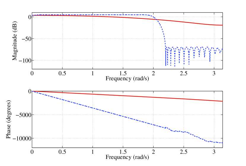
Since the conventional theory requires to perfectly cut off the frequency response beyond the frequency $2/3\pi$ (rad/s), the resulting filter shows a very sharp decay beyond this frequency. On the other hand, our filter shows much slower decay. To see this difference, we show in Fig.ย 10 the frequency responses of the error system $T_{ew}(\widetilde{{\mathcal{K}}},{\mathbf{M}})$ in Fig.ย 4.

Refer to caption
Figure 10. Frequency response: proposed (solid) and conventional (dots).

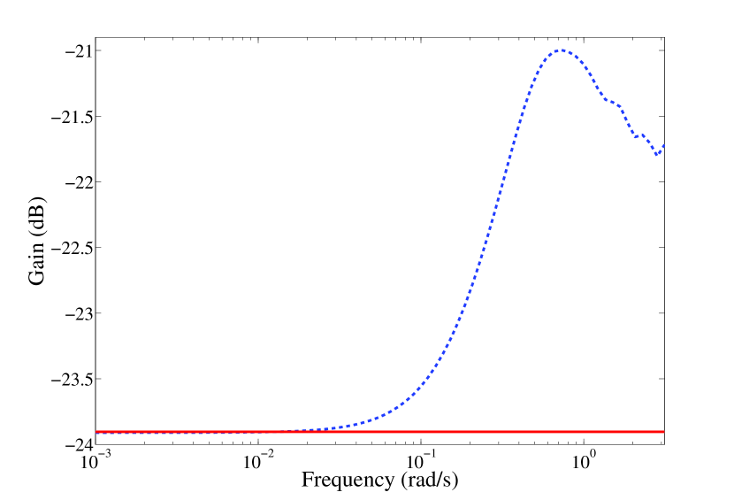
The conventional interpolation shows a large error in high frequency, while the sampled-data $H^{\infty}$ optimal interpolation shows a flat response.

To illustrate the difference between these frequency responses, we simulate interpolation of a rectangular wave. Figure 11 shows the time response.

Refer to caption
Figure 11. Time response: proposed (solid), conventional (dash), and input signal(dots).

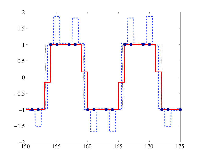
The conventional interpolation causes large ripples, while our interpolation shows a better response. This is because the rectangular wave has high frequency components around the edges, and our interpolation takes account of such frequency components. Figure 12 shows the absolute errors.

Refer to caption
Figure 12. Absolute Error in the time response in Fig.ย 11: proposed (solid) and conventional (dash).

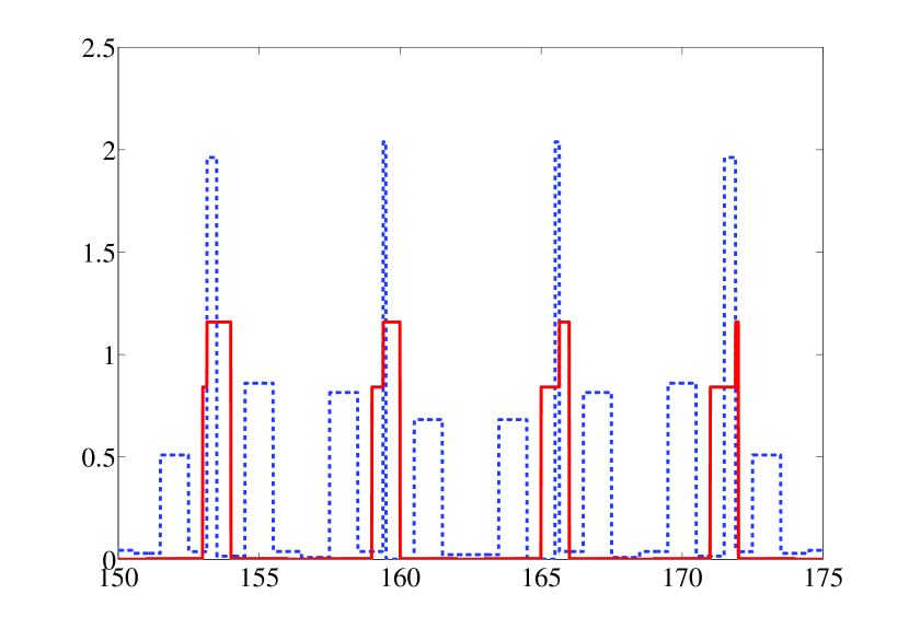
We can see that our response shows smaller errors than the conventional design.

5.2. Decimation Pattern Analysis

Here we find the optimal decimation patterns for given decimation ratio $M/N$. The sampling period is assumed to be $h=1$. The transfer function Fโ€‹(s)๐น๐‘ F(s) is given by (12). The reconstruction delay is set $L=M$ (the length of ${\mathbf{M}}$).

First, Let $M=4$ and $N=2$. In this case, the essential patterns are ${\mathbf{M}}=[1,1,0,0]$ and ${\mathbf{M}}=[1,0,1,0]$. Tableย 1 shows the optimal value $J({\mathbf{M}})$ defined in (11).

Table 1. Optimal value $J({\mathbf{M}})$ for $M=4$ and $N=2$
Decimation Pattern $J({\mathbf{M}})$
0.2293
${\mathbf{M}}=[1100]$, $[1001]$, $[0110]$, $[0011]$
0.1529
${\mathbf{M}}=[1010]$, $[0101]$

We can see the difference between the two patterns with the same decimation ratio. This result shows that the pattern ${\mathbf{M}}=[1,0,1,0]$ (or ${\mathbf{M}}=[0,1,0,1]$) is the better, which is equal to the uniform decimation $\downarrow\!2$.

We then consider when the segment length $M=5$. Tableย 2 shows the result. By this, the optimal value $J({\mathbf{M}})$ depends on the position of the zeros in ${\mathbf{M}}$, not depends on the number of the ones in ${\mathbf{M}}$. For example, although the pattern (F) retains more samples than the pattern (E), the optimal values are the same. This fact shows that a lower ratio of decimation (or compression) does not necessarily lead to a better performance. In other words, not only decimation ratio but also decimation pattern plays an important role in signal compression.

Table 2. Optimal value $J({\mathbf{M}})$ for $M=5$ and $N=1,2,3,4$
Pattern $J({\mathbf{M}})$ Pattern $J({\mathbf{M}})$
0.3813 0.2303
(A) (D)
0.3062 0.1536
(B) (E)
0.2303 0.1536
(C) (F)

Tableย 3 shows the optimal $J({\mathbf{M}})$ when $M=7$ and $N=4$, that is, the decimation ratio is $7/4$.

Table 3. Optimal value $J({\mathbf{M}})$ for $M=7$, $N=4$.
Decimation Pattern $J({\mathbf{M}})$
0.3089
(A)
(B)
0.2320
(C)
(D)
0.1547
(E)

In this case, there are 5 essential patterns (A) to (E). We can see that the best pattern is (E). We can also see that $J({\mathbf{M}})$ depends on the maximal number of the consecutive zeros in ${\mathbf{M}}$ (we here call this the consecutive number).

These results shows that the optimal value of $J({\mathbf{M}})$ depends on the consecutive number and not on the number of retained samples. By this observation, we can make a hypothesis that the optimal decimation pattern ${\mathbf{M}}$ is the pattern in which the zeros are the least consecutive. In other words, the most uniformly distributed pattern is the best. In view of this, the block decimation introduced in [8] cannot be optimal. Note that the hypothesis does not detract from the merit of nonuniform decimation; if the ratio $M/N$ is non integer, nonuniform decimation is inevitable.

6. Conclusion

We have proposed an interpolation method of nonuniform decimation for non-band-limited signals. To design the interpolation system, we adopt the $H^{\infty}$ norm of the error system. We have shown that the optimization can be efficiently executed by numerical computation. We have also considered designing decimation pattern with the $H^{\infty}$ optimal performance index. Design examples have shown the effectiveness of the present method. A theoretical proof for the hypothesis given in Subsection 5.2 remains an open question.

References

  • [1] T.ย Chen and B.ย Francis: Optimal Sampled-Data Control Systems,ย ย ย Springer, 1995.
  • [2] R.ย Klette and P.ย Zamperoni: Handbook of Image Processing Operators,ย ย ย John Wiley & Sons, 1996.
  • [3] Y.-P. Lin and P.ย P. Vaidyanathan: Periodically nonuniform sampling of bandpass signals, IEEE Trans. Circuits Syst. II, Vol.ย 45, No.ย 3, 1998.
  • [4] R.ย J. Marks II and S.ย Narayanan: Interpolation of discrete periodic nonuniform decimation using alias unraveling, Proc.ย of 2002 IEEE Int.ย Symp.ย Circuits Syst., pp. 281โ€“284, 2002.
  • [5] D.ย G. Meyer: A parametrization of stabilizing controllers for multirate sampled-data systems, IEEE Trans. Automat. Contr., Vol.ย 35, No.ย 2, pp.ย 233โ€“236, 1990.
  • [6] M.ย Nagahara and Y.ย Yamamoto: A new design for sample-rate converters, Proc.ย of 39th IEEE Conf.ย Decision and Control, pp. 4296โ€“4301, 2000.
  • [7] M.ย Nagahara, Y.ย Yamamoto, and P.ย P. Khargonekar: Stability of signal reconstruction filters via cardinal exponential splines, Proc.ย of 17th IFAC World Congress, pp. 1414โ€“1419, 2008.
  • [8] K.ย Nayebi, T.ย P. Barnwell III, and M.ย J.ย T. Smith: Nonuniform filter banks: A reconstruction and design theory, IEEE Trans. Signal Processing, Vol.ย 41, No.ย 3, pp. 1114โ€“1127, 1993.
  • [9] S.ย C. Park, M.ย K. Park, and M.ย G. Kang: Super-resolution image reconstruction: A technical overview, IEEE Signal Processing Mag., Vol.ย 20, No.ย 3, pp. 21โ€“36, 2003.
  • [10] T.ย Strohmer and J.ย Tanner: Fast reconstruction algorithms for periodic nonuniform sampling with applications to time-interleaved ADCs, Proc.ย of 2007 Int.ย Conf.ย Acoust., Speech, Signal Processing, Vol.ย 3, pp. 881โ€“884, 2007.
  • [11] M.ย Unser: Cardinal exponential splines: Part ii โ€” think analog, act digital, IEEE Trans. Signal Processing, Vol.ย 53, No.ย 4, pp. 1439โ€“1449, 2005.
  • [12] M.ย Unser and J.ย Zerubia: A generalized sampling theory without band-limiting constraints, IEEE Trans. Circuits Syst. II, Vol.ย 45, No.ย 8, pp. 959โ€“969, 1998.
  • [13] P.ย P. Vaidyanathan: Multirate Systems and Filter Banks,ย ย ย Prentice Hall, 1993.
  • [14] P.ย P. Vaidyanathan and V.ย C. Liu: Efficient reconstruction of band-limited sequences from nonuniformly decimated versions by use of polyphase filter banks, IEEE Trans. Acoust., Speech, Signal Processing, Vol.ย 38, No.ย 11, pp. 1927โ€“1936, 1990.
  • [15] L.ย Vandendorpe, P.ย Delogne, B.ย Maison, and L.ย Cuvelier: MMSE design of interpolation and downsampling FIR filters in the context of periodic nonuniform sampling, IEEE Trans. Signal Processing, Vol.ย 45, No.ย 5, 1997.
  • [16] Y.ย Yamamoto, B. D. O. Anderson, and M.ย Nagahara: Approximating sampled-data systems with applications to digital redesign, Proc.ย of 41st IEEE Conf.ย Decision and Control, pp. 3724โ€“3729, 2002.
  • [17] Y. Yamamoto, B. D. O. Anderson, M. Nagahara, and Y. Koyanagi: Optimizing FIR approximation for discrete-time IIR filters, IEEE Signal Processing Lett., Vol.ย 10, No.ย 9, pp.ย 273โ€“276, 2003.
  • [18] Y.ย Yamamoto, A.ย G. Madievski, and B.ย D.ย O. Anderson: Approximation of frequency response for sampled-data control systems, Automatica, Vol.ย 35, No.ย 4, pp. 729โ€“734, 1999.
  • [19] Y.ย Zimmels and L.ย G.ย Fel: Multinomial permutations on a circle, Math.ย Meth.ย Appl.ย Sci., Vol.ย 29, No.ย 17, pp.ย 2079โ€“2088, 2006.
  • [20] http:โ€‹/โ€‹/www-ics.acs.i.kyoto-u.ac.jp/~nagahara/nui/