$H^{\infty}$ Optimal Approximation for Causal Spline Interpolation

Abstract.

In this paper, we give a causal solution to the problem of spline interpolation using $H^{\infty}$ optimal approximation. Generally speaking, spline interpolation requires filtering the whole sampled data, the past and the future, to reconstruct the inter-sample values. This leads to non-causality of the filter, and this becomes a critical issue for real-time applications. Our objective here is to derive a causal system which approximates spline interpolation by $H^{\infty}$ optimization for the filter. The advantage of $H^{\infty}$ optimization is that it can address uncertainty in the input signals to be interpolated in design, and hence the optimized system has robustness property against signal uncertainty. We give a closed-form solution to the $H^{\infty}$ optimization in the case of the cubic splines. For higher-order splines, the optimal filter can be effectively solved by a numerical computation. We also show that the optimal FIR (Finite Impulse Response) filter can be designed by an LMI (Linear Matrix Inequality), which can also be effectively solved numerically. A design example is presented to illustrate the result.

1. Introduction

Splines are widely used in image processing due to their simple mathematical structure, in particular, linearity and low complexity in computation. Interpolation with these splines, called spline interpolation, provides smoothness, that is, the interpolated function can be continuous and several times differentiable. By these advantages, polynomial splines are very popular in image processing such as curve fitting [11], image interpolation (zooming) [9], rotation [19], compression [6], and super resolution [1].

Theoretically, spline interpolation provides perfect fitting for given sampled data when the original analog signal is in the spline space [10, 14, 15]. This ideal spline interpolant is however obtained by filtering the whole sampled data. This leads to non-causality of the interpolation process. Although this non-causality is not a restriction for image processing, spline interpolation cannot be used for real-time processing such as instrumentation or audio/speech processing. When spline interpolation is used in AD (Analog-to-Digital) and DA (Digital-to-Analog) converters [13], and when it is used in a feedback loop, the reconstruction delay degrades the stability and the performance of the system. In this case, the real-time processing is crucial.

For this non-causality problem, various approximation methods have been proposed to obtain a causal system which approximates the ideal (non-causal) spline interpolation, by the constrained least square design [18], the Kaiser window method [20], and the maximum order minimum support (MOMS) function method [3]. These methods are based on minimizing the squared approximation error in the time domain. This optimization can be generalized to $H^{2}$ optimization [24].

$H^{2}$ optimization minimizes the $\ell^{2}$ norm of the impulse response. Hence it works basically for this particular signal only, and its performance against other input signals is not a priori guaranteed. In other words, it can happen that the reconstruction error will be significantly large for other unknown signals. In real systems, input signals are unknown, or only partially known (e.g., the input signals contain their frequencies mostly within 1.5 rad/sec), and hence there are uncertainty in input signals. To model such uncertainty, we assume a certain class of input function spaces, and consider a neighborhood (e.g., a unit ball) of such a function space. We then consider that signal uncertainty as nominal signal plus unknown signals that belongs to such a ball. By controlling the induced norm of a pertinent operator, one can attenuate the response against such uncertainty, and this provides a contrasting viewpoint of robustness, not in a probabilistic sense, but in a deterministic treatment. This has the advantage of minimizing the worst-case errors in contrast to probabilist models. Robustness against such uncertainty is achieved by $H^{\infty}$ optimization [24] which aims at minimizing or maintaining the error level below a certain prescribed performance level against all input signals, and possess much higher robustness against lack of a priori knowledge about input signals to be processed.

$H^{\infty}$ optimization was first proposed and developed in control theory [23], and then applied to signal processing [5, 22, 7]. Since the $H^{\infty}$ norm gives the $\ell^{2}$-induced norm or the maximum energy gain, minimizing the $H^{\infty}$ norm of the error system gives the optimality for the worst case. This property leads to robustness of the system against uncertainty of the input signal. That is, the $H^{\infty}$ design guarantees an error level $\gamma$ for all $\ell^{2}$ signals. Moreover, the $H^{\infty}$ method can naturally take a frequency weight in the design. The weight can control the shape of the frequency response of the error system, according to given knowledge on the frequency characteristic of the input signals. From the computation viewpoint, the $H^{\infty}$ optimization can be executed numerically via the state-space formulation, and is easily done by standard softwares, as MATLAB.

We propose a new approximation method for causal spline interpolation by $H^{\infty}$ optimization. The design is formulated as obtaining the $H^{\infty}$-sub-optimal stable inverse filter of a system with unstable zeros. In particular, for the cubic spline (3rd order spline), the $H^{\infty}$ optimal filter can be obtained in a closed form. For a spline with arbitrary order, the $H^{\infty}$ sub-optimal IIR (Infinite Impulse Response) filter is easily obtained by numerical computation. Moreover, by confining the desired sub-optimal filter to be FIR (Finite Impulse Response), the optimization is reducible to an LMI (Linear Matrix Inequality), which can be effectively solved by, for example, standard MATLAB routines. A design example is presented to show effectiveness of our method.

The paper is organized as follows. In Section 2, we introduce spline interpolation. In Section 3, we formulate our problem by $H^{\infty}$ optimization, and derive the solution. Performance analysis of our spline interpolation system is discussed in Section 4. Section 5 shows a design example and Section 6 concludes our result.

Notation

Throughout this paper, we use the following notation.

${\mathbb{Z}}$, ${\mathbb{Z}}_{+}$:

: the sets of integers and non-negative integers, respectively.

${\mathbb{R}}$, ${\mathbb{R}}_{+}$:

: the sets of real numbers and non-negative real numbers, respectively.

$\mathbb{C}$:

the complex plane.

${\mathcal{D}}$:

the open unit disc in $\mathbb{C}$.

$\mathbf{C}^{N}$:

the set of continuous functions with continuous derivatives up to order $N$.

$P_{N}$:

the set of polynomial functions whose order is equal or less than $N$.

$S_{N}$:

the set of $\mathbf{C}^{N}$ functions whose restriction on $[n,n+1)$, $n\in{\mathbb{Z}}$ is in $P_{N}$, that is, on each interval $[n,n+1)$ the $S_{N}$ function is a polynomial whose order is equal or less than $N$.

$L^{2}(X)$:

the Lebesgue space consisting of all square integrable real functions on $X$. $L^{2}({\mathbb{R}}_{+})$ is abbreviated to $L^{2}$.

$\ell^{2}(X)$:

the set of all real-valued square summable sequences on $X$. $\ell^{2}({\mathbb{Z}}_{+})$ is abbreviated to $\ell^{2}$.

$\delta$:

the discrete-time impulse or the Kronecker delta, that is, $\delta(n)=1$, if $n=0$, and $0$, otherwise.

$\phi\ast\psi$:

convolution of a sequence $\{\phi(n)\}_{n\in{\mathbb{Z}}}$ and $\{\psi(n)\}_{n\in{\mathbb{Z}}}$, that is,

$$(\phi\ast\psi)(n)=\sum_{n\in{\mathbb{Z}}}\phi(n-k)\ast\psi(k),\quad n\in{\mathbb{Z}}.$$

$\sigma$, $\sigma^{-1}$:

the forward and backward shift operator, respectively. That is, for a sequence $\{x(n)\}_{n\in{\mathbb{Z}}}$, $(\sigma\ast x)(n)=x(n+1)$ and $(\sigma^{-1}\ast x)(n)=x(n-1)$.

$z$, $z^{-1}$:

the $Z$-transform of $\sigma$ and $\sigma^{-1}$, respectively. For a sequence $\{x(n)\}_{n\in{\mathbb{Z}}}$, the $Z$-transform $\hat{x}$ of $x$ is defined by

$$\hat{x}(z):=\sum_{n=-\infty}^{\infty}x(n)z^{-n}.$$

$A^{\top}$:

the transpose of a matrix $A$.

$I_{M}$, $0_{M\times N}$:

the $M\times M$ identity matrix and the $M\times N$ zero matrix, respectively.

2. Spline interpolation

We here discuss polynomial spline interpolation. In this paper, we consider the cardinal interpolation problem [10]:

Problem 1.

Given a sequence $\{x(n)\}_{n\in{\mathbb{Z}}}$, construct a function $y(t)$, $t\in{\mathbb{R}}$ satisfying the relation

$$y(n)=x(n),\quad n\in{\mathbb{Z}}.$$

Needless to say, this problem is ill-posed because there are infinitely many solutions. To obtain a unique solution, one should specify the space to which the original signal $\{x(t)\}_{t\in{\mathbb{R}}}$ belongs. Assume that the space is

$$V=\left\{x\in L^{2}({\mathbb{R}}):{\text{supp}}(\widehat{x})\subseteq[-\pi,\pi]\right\},$$

where $L^{2}({\mathbb{R}})$ is the Lebesgue space of all square integrable functions on ${\mathbb{R}}$, and $\widehat{x}$ is the Fourier transform of $x$. Then, we have the well known solution called cardinal sinc series [10, 14],

$$y(t)=\sum_{n\in{\mathbb{Z}}}x(n)\frac{\sin\pi(t-n)}{\pi(t-n)},\quad t\in{\mathbb{R}}.$$

That is, for any $x\in V$, we have $y(t)=x(t)$ for all $t\in{\mathbb{R}}$.

On the other hand, assume that the space is

$$S_{N}=\left\{x\in\mathbf{C}^{N}:x|_{[n,n+1)}\in P_{N},n\in{\mathbb{Z}}\right\},$$ (1)

where $\mathbf{C}^{N}$ is the set of continuous functions with continuous derivatives up to order $N$. Then the solution is given by [10],

$$y(t)=\sum_{n\in{\mathbb{Z}}}c(n)\phi(t-n),\quad t\in{\mathbb{R}},$$ (2)

where $\phi$ is the polynomial B-spline basis defined by [10, 15],

$$\begin{split}\phi(t)=(\underbrace{\beta^{0}\ast\cdots\ast\beta^{0}}_{N+1})(t),\quad\beta^{0}(t)=\begin{cases}1,&0\leq t\leq 1,\\ 0,&\text{otherwise,}\end{cases}\end{split}$$

where ‘$\ast$’ denotes convolution. Figure 1 shows the polynomial splines $\phi(t)$ of order $N=0,1,2,3$.

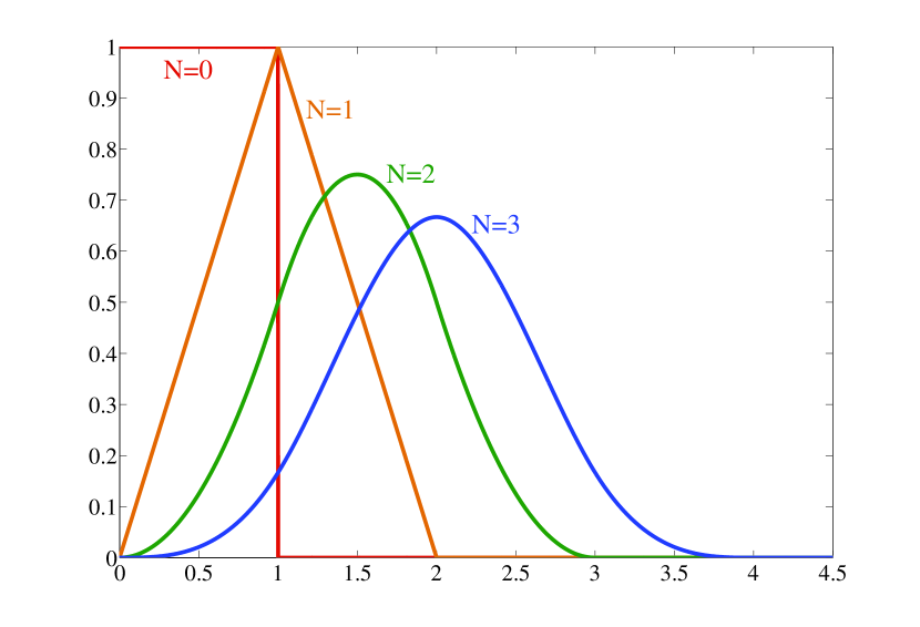
Figure 1. Polynomial spline of order $N=0,1,2,3$

In this formulation, the coefficients are given by the following convolution formula [15]:

$$c(n)=(\psi\ast x)(n),\quad n\in{\mathbb{Z}},$$ (3)

where $\psi$ is the direct B-spline filter satisfying $\psi\ast\phi=\delta$, or in $Z$-transform,

$$\psi(z)\phi(z)=1.$$ (4)

This is for the perfect reconstruction without any delay. If we allow a delay $d>0$ for reconstruction, the condition becomes $\psi\ast\phi=\sigma^{-d}$, where $\sigma^{-d}$ is the $d$-step delay, or the inverse $Z$-transform of $z^{-d}$, that is,

$$\psi(z)\phi(z)=z^{-d}.$$ (5)

3. Causal spline interpolation by $H^{\infty}$ optimization

3.1. Standard non-causal interpolation

Since the $N$th-order spline $\phi(t)$ is supported in $[0,N+1)$, the sampled signal $\phi(n)$ is represented as an FIR (finite impulse response) filter. For example, in the case of $N=3$ (cubic spline), we have

$$\phi(z)=\frac{1}{6}+\frac{2}{3}z^{-1}+\frac{1}{6}z^{-2}.$$ (6)

By (4), the desired filter $\psi(z)$ is given by the inverse $\psi=\phi^{-1}$ and it is seen that

$$\psi(z)=\frac{6}{z^{-2}+4z^{-1}+1}.$$

One of the poles of $\psi(z)$ lies out of the open unit disc $\mathcal{D}:=\{z\in\mathbb{C}:|z|<1\}$, and hence the filter $\psi(z)$ becomes unstable. The same can be said of the other $N$th-order splines [16]. A practical way to implement this filter is to decompose $\psi(z)$ into a cascade of causal and anti-causal filters [16]. In the case of the cubic spline, we first shift the impulse response of (6) as

$$z\phi(z)=\frac{1}{6}z+\frac{2}{3}+\frac{1}{6}z^{-1},$$

and then decompose $\psi(z)=[z\phi(z)]^{-1}$ as

$$\psi(z)=-\frac{6\alpha}{1-\alpha^{2}}\left(\frac{1}{1-\alpha z^{-1}}+\frac{1}{1-\alpha z}-1\right),$$ (7)

where $\alpha=-2+\sqrt{3}$. Since $|\alpha|<1$, this is a stable and non-causal IIR (infinite impulse response) filter. Figure 2 shows the impulse response of this non-causal filter.

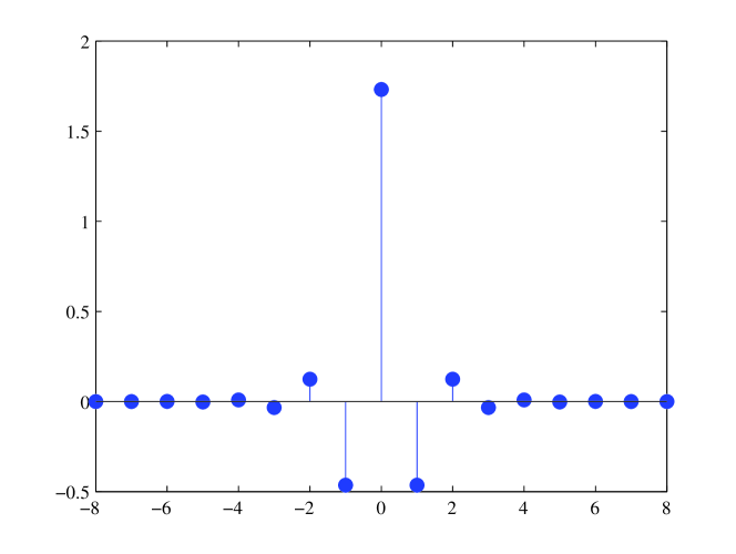
Figure 2. Impulse response of non-causal filter $\psi(z)=6/(z+4+z^{-1})$

3.2. Causal interpolation by $H^{\infty}$ optimization

In image processing, causality is often of secondary importance, and non-causal filters as above are used widely in that field, by suitably reversing the part of time axis as above. However, for real-time processing this is not quite appropriate, for example, in instrumentation or audio/speech processing. To process such a signal, it takes infinite time or at least time propotional to the length of the signal since the non-causal filter $\psi(z)$ in (7) has infinite taps. We propose a design of a causal filter $\psi(z)$ which approximates the condition (5) of delayed perfect reconstruction, allowing a (small) time delay. Our problem is the following:

Problem 2.

Given a stable transfer function $\phi(z)$, a stable weighting transfer function $w(z)$, and delay $d\geq 0$, find a causal and stable filter $\psi(z)$ which minimizes

$$\begin{split}J(\psi)&=\left\|\left\{z^{-d}-\psi(z)\phi(z)\right\}w(z)\right\|_{\infty}\\ &=\max_{\theta\in[0,2\pi)}\left|\left\{e^{-jd\theta}-\psi(e^{j\theta})\phi(e^{j\theta})\right\}w(e^{j\theta})\right|.\end{split}$$ (8)

This is a standard $H^{\infty}$ optimization problem, and it can be effectively solved by standard MATLAB routines (e.g., dhfsyn in MATLAB robust control toolbox [2]) by using the block diagram shown in Figure 3. The MATLAB code for solving Problem 2 is available in [25].

Figure 3. Block diagram for $H^{\infty}$ optimization

3.3. $H^{\infty}$ optimal cubic spline

The cubic spline ($N=3$) is widely used because of its simple structure; for example, the cubic spline is the lowest-order spline for which the knot-discontinuity is not visible to the human eye [8]. Moreover, the cubic spline has minimum curvature property [13], that is, the cubic spline minimizes

$$\int_{\mathbb{R}}\left|y^{\prime\prime}(t)\right|^{2}\mathrm{d}t,$$

the $L^{2}$ norm of the curvature of the interpolated signal $y(t)$ in (2). While the $H^{\infty}$ filter above can be effectively computed via various numerical methods, it is even possible to give a closed-form formula for the case of the cubic spline which is widely used in digital signal processing.

Assume $w(z)=1$ and define

$$E(z):=z^{-d}-\psi(z)\phi(z).$$

Substituting (6) into this equation, we have

$$E(z)=z^{-d}-\psi(z)\frac{(z-\alpha_{1})(z-\alpha_{2})}{6z^{2}},$$

$$\alpha_{1}:=-2-\sqrt{3},\quad\alpha_{2}:=-2+\sqrt{3}.$$

This equation gives

$$\psi(z)=\frac{6z^{2}(z^{-d}-E(z))}{(z-\alpha_{1})(z-\alpha_{2})}.$$

Since $|\alpha_{1}|>1$, the filter $\psi(z)$ may have a pole outside the open unit disc ${\mathcal{D}}$. It is easily shown that the filter $\psi(z)$ is stable (i.e., all poles of $\psi(z)$ lie in $\mathcal{D}$) if and only if

$$E(\alpha_{1})=\alpha_{1}^{-d}.$$ (9)

Then our problem is to find a stable $E(z)$ of minimum $H^{\infty}$ norm under the interpolation constraint (9). This is a Nevanlinna-Pick interpolation problem [21]. By the maximum modulus principle, we have

$$\|E\|_{\infty}=\sup_{|z|=1}|E(z)|=\sup_{|z|\geq 1}|E(z)|\geq|E(\alpha_{1})|=|\alpha_{1}^{-d}|.$$

The interpolating function of minimum $H^{\infty}$ norm is therefore the constant function $E(z)=\alpha_{1}^{-d}$. By this, we obtain the optimal $\psi(z)$ as follows:

$$\begin{split}\psi(z)&=\frac{6z^{2}}{(z-\alpha_{1})(z-\alpha_{2})}(z^{-d}-\alpha_{1}^{-d})\\ &=-\frac{6z^{2}}{\alpha_{1}^{d}z^{d}(z-\alpha_{2})}\sum_{k=0}^{d-1}\alpha_{1}^{d-1-k}z^{k}.\end{split}$$ (10)

We summarize the result as a proposition.

Proposition 1.

For given $d\geq 0$ and the cubic spline function $\phi(z)$ in (6), the $H^{\infty}$ optimal $\psi(z)$ which minimizes $J(\psi)=\|E\|_{\infty}$ is given by

$$\psi(z)=-\frac{6z^{2}}{\alpha_{1}^{d}z^{d}(z-\alpha_{2})}\sum_{k=0}^{d-1}\alpha_{1}^{d-1-k}z^{k},$$ (11)

and the optimal value $\min_{\psi}J(\psi)=|\alpha_{1}^{-d}|$.

Remark 1.

For higher-order splines (i.e., $N\geq 4$), the optimal filter can be obtained by the Nevanlinna algorithm [21]. A closed-form solution is however very complicated when $N\geq 4$. In that case, the numerical computation shown in 3.2 or 3.4 is available.

3.4. FIR filter design via LMI

The $H^{\infty}$-optimal filter is generally an IIR one. We here propose a design of the $H^{\infty}$-suboptimal FIR filter (with arbitrarily specified performance close to optimality). Assume that the direct filter $\psi(z)$ is FIR, that is,

$$\psi(z)=\sum_{m=0}^{M}a_{m}z^{-m}.$$

We here represent systems in a state space. By the state-space formalism, we can reduce the computation of $H^{\infty}$ optimization to a linear matrix inequality (LMI).

A state-space representation of the FIR filter $\psi(z)$ is given by

$$\begin{split}\psi(z)&=\left[\begin{array}[]{ccccc|c}0&1&0&\ldots&0&0\\ \vdots&\ddots&\ddots&\ddots&\vdots&\vdots\\ \vdots&&\ddots&\ddots&0&0\\ \vdots&&&\ddots&1&0\\ 0&\ldots&\ldots&\ldots&0&1\\ \hline\cr a_{M}&\ldots&\ldots&\ldots&a_{1}&a_{0}\end{array}\right](z)\\ &=:\left[\begin{array}[]{c|c}A_{\psi}&B_{\psi}\\ \hline\cr C_{\psi}({\boldsymbol{a}})&D_{\psi}({\boldsymbol{a}})\end{array}\right](z),\end{split}$$

where ${\boldsymbol{a}}:=\left[\begin{array}[]{cccc}a_{M}&\ldots&a_{1}&a_{0}\end{array}\right]^{\top}$, and we use the notation by Doyle [24]:

$$\left[\begin{array}[]{c|c}A&B\\ \hline\cr C&D\\ \end{array}\right](z):=C(zI-A)^{-1}B+D.$$

Note that the parameter vector ${\boldsymbol{a}}$ to be designed is linearly dependent only on the matrices $C_{\psi}({\boldsymbol{a}})$ and $D_{\psi}({\boldsymbol{a}})$, that is, $C_{\psi}({\boldsymbol{a}})={\boldsymbol{a}}^{\top}V_{C}$ and $D_{\psi}({\boldsymbol{a}})={\boldsymbol{a}}^{\top}V_{D}$, where

$$V_{C}=\left[\begin{array}[]{c}I_{M}\\ 0_{1\times M}\end{array}\right],\quad V_{D}=\left[\begin{array}[]{c}0_{M\times 1}\\ 1\end{array}\right].$$

Set state-space representations of $\phi(z)w(z)$ and $z^{-d}w(z)$ respectively by

$$\begin{split}\phi(z)w(z)&=:\left[\begin{array}[]{c|c}A_{\phi}&B_{\phi}\\ \hline\cr C_{\phi}&D_{\phi}\end{array}\right](z),\quad\\ z^{-d}w(z)&=:\left[\begin{array}[]{c|c}A_{d}&B_{d}\\ \hline\cr C_{d}&0\end{array}\right](z).\end{split}$$

Then, a state-space representation of the error system

$$E_{w}(z):=\left\{z^{-d}-\psi(z)\phi(z)\right\}w(z)$$

is given by

$$\begin{split}E_{w}(z)&=\left[\begin{array}[]{ccc|c}A_{\psi}&B_{\psi}C_{\phi}&0&-B_{\psi}D_{\phi}\\ 0&A_{\phi}&0&-B_{\phi}\\ 0&0&A_{d}&B_{d}\\ \hline\cr C_{\psi}({\boldsymbol{a}})&D_{\psi}({\boldsymbol{a}})C_{\phi}&C_{d}&-D_{\psi}({\boldsymbol{a}})D_{\phi}\end{array}\right](z)\\ &=:\left[\begin{array}[]{c|c}A&B\\ \hline\cr C({\boldsymbol{a}})&D({\boldsymbol{a}})\end{array}\right](z).\end{split}$$

By this, the parameter ${\boldsymbol{a}}$ to be designed is affinely dependent only on the matrices $C({\boldsymbol{a}})$ and $D({\boldsymbol{a}})$, that is,

$$\begin{split}C({\boldsymbol{a}})&={\boldsymbol{a}}^{\top}\begin{bmatrix}V_{C}&V_{D}C_{\phi}&0_{1\times d}\end{bmatrix}+\begin{bmatrix}0_{1\times(M+N-1)}&C_{d}\end{bmatrix},\\ D({\boldsymbol{a}})&=-{\boldsymbol{a}}^{\top}V_{D}D_{\phi},\end{split}$$

where $N$ is the order of the B-spline basis $\phi$. By using the bounded real lemma or Kalman-Yakubovic-Popov (KYP) lemma, we can describe our design problem as an LMI [22].

Proposition 2.

Let $\gamma$ be a positive number. Then the inequality $\|E_{w}(z)\|_{\infty}<\gamma$ holds if and only if there exist a positive definite matrix $P>0$ such that

$$\left[\begin{array}[]{ccc}A^{\top}PA-P&A^{\top}PB&C({\boldsymbol{a}})^{\top}\\ B^{\top}PA&-\gamma I+B^{\top}PB&D({\boldsymbol{a}})^{\top}\\ C({\boldsymbol{a}})&D({\boldsymbol{a}})&-\gamma I\end{array}\right]<0.$$ (12)

Remark 2.

In some applications, the error system $E_{w}(z)$ is required to have specified zeros $z_{i}\in\mathbb{C}$, $i=1,2,\ldots,L$. In particular, zero-bias constraint (i.e., $E_{w}(1)=0$ ) is used for perfect reconstruction of DC (direct current) signals [18]. In such cases, zeros of $E_{w}(z)$ can be set by

$$C({\boldsymbol{a}})(z_{i}I-A)^{-1}B+D({\boldsymbol{a}})=0,\quad i=1,2,\ldots,L.$$

These are linear matrix equations with respect to the design parameter ${\boldsymbol{a}}$. The LMI (12) combined with these linear constraints is also easily solvable via standard MATLAB routines.

Remark 3.

To obtain the optimal ${\boldsymbol{a}}$, minimize $\gamma$ subject to the LMI (12). This minimization is also easily executed by MATLAB. The MATLAB code for this optimization is available in [25].

4. Performance analysis

In the previous section, we have proposed the $H^{\infty}$ optimization design of the filter $\phi(z)$ which approximates the delayed perfect reconstruction condition (5). In this section, we analyze the overall performance of the interpolation system shown in Figure 4.

Figure 4. Signal Interpolation System

In Figure 4, $\mathcal{S}$ is the ideal sampler defined by

$$\mathcal{S}:\{x(t)\}_{t\in{\mathbb{R}}_{+}}\mapsto\{x(n)\}_{n\in{\mathbb{Z}}_{+}},$$

and $\mathcal{H}_{\phi}$ is a hold defined by

$$\mathcal{H}_{\phi}:\{c(n)\}_{n\in{\mathbb{Z}}_{+}}\mapsto\left\{\sum_{n=0}^{\infty}c(n)\phi(t-n)\right\}_{t\in{\mathbb{R}}_{+}}.$$

For simplicity, we set $w(z)=1$ in this section. Then we show that the approximation of the equation (5) is proper for decreasing the NSR (noise-to-signal ratio) of the interpolation system.

Proposition 3.

Assume that $\phi$ and $\psi$ are causal and stable. Let $x$ be in $S_{N}\cap L^{2}$ and $y$ be the reconstructed signal by the direct B-spline transform $\psi$, that is,

$$y(t)=\sum_{n=0}^{\infty}(\psi\ast x)(n)\phi(t-n),\quad t\in{\mathbb{R}}_{+}.$$

Then there exists a real number $\lambda>0$ which depends only on $\phi$ such that for any non-negative integer $d$,

$$\frac{\|x(\cdot-d)-y\|_{L^{2}}}{\|x\|_{L^{2}}}\leq\lambda J(\psi).$$

Proof. Since $x\in S_{N}$, there exists a sequence $\{c(n)\}_{n\in{\mathbb{Z}}_{+}}$ such that

$$x(t)=\sum_{n=0}^{\infty}c(n)\phi(t-n).$$

We define $c(n)=0$ for $n<0$. Then, for arbitrary fixed integer $d\geq 0$, we have

$$\begin{split}&x(t-d)-y(t)\\ &\quad=\sum_{n=0}^{\infty}\left\{c(n)\phi(t-d-n)-(\psi\ast x)(n)\phi(t-n)\right\}\\ &\quad=\sum_{n=0}^{\infty}\left\{c(n-d)-(\psi\ast x)(n)\right\}\phi(t-n)\\ &\quad=\sum_{n=0}^{\infty}\left\{c(n-d)-(\psi\ast\phi\ast c)(n)\right\}\phi(t-n)\\ &\quad=\sum_{n=0}^{\infty}\left\{(\sigma^{-d}-\psi\ast\phi)\ast c\right\}(n)\phi(t-n)\\ &\quad=\sum_{n=0}^{\infty}(e\ast c)(n)\phi(t-n),\end{split}$$

where $e:=\sigma^{-d}-\psi\ast\phi$. Then, since $\phi$ is a Riesz basis [12], there exist $a>0$ and $b>0$ such that for any $c\in\ell^{2}$,

$$a\|c\|_{\ell^{2}}\leq\left\|\sum_{n=0}^{\infty}c(n)\phi(t-n)\right\|_{L^{2}}\leq b\|c\|_{\ell^{2}}.$$

By using this inequality, we have

$$\begin{split}\|x(\cdot-d)-y\|_{L^{2}}&=\left\|\sum_{n=0}^{\infty}(e\ast c)(n)\phi(\cdot-n)\right\|_{L^{2}}\\ &\leq b\|e\ast c\|_{\ell^{2}}\\ &\leq b\|z^{-d}-\psi(z)\phi(z)\|_{\infty}\|c\|_{\ell^{2}}\\ &\leq\frac{b}{a}\|z^{-d}-\psi(z)\phi(z)\|_{\infty}\|x\|_{L^{2}}.\end{split}$$

Since $J(\psi)=\|z^{-d}-\psi(z)\phi(z)\|_{\infty}$, we have

$$\frac{\|x(\cdot-d)-y\|_{L^{2}}}{\|x\|_{L^{2}}}\leq\lambda J(\psi),$$

where $\lambda=b/a>0$, which depends only on $\phi$. $\Box$

We thus conclude that if the $H^{\infty}$ norm of the error system $z^{-d}-\phi(z)\psi(z)$ is adequately small, the NSR of the interpolator can be decreased, and hence $H^{\infty}$ optimization provides a good approximation of the ideal (i.e., non-causal) spline interpolation.

We next consider a relation between our causal approximation and the ideal noncausal interpolation. The following corollary to Proposition 3 guarantees that our approximation recovers the ideal interpolation (i.e., perfect fitting) when the delay $d$ goes to infinity.

Corollary 1.

Let $RH^{\infty}$ be the set of all real, stable and causal IIR filters. Then, for any $x\in S_{N}\cap L^{2}$ we have

$$\inf_{\psi\in RH^{\infty}}\frac{\|x(\cdot-d)-y\|_{L^{2}}}{\|x\|_{L^{2}}}\rightarrow 0,\quad\text{as }d\rightarrow\infty$$ (13)

Proof. Let $J_{\text{opt}}(d)$ be the optimal value of $J(\psi)$, that is,

$$J_{\text{opt}}(d):=\inf_{\psi\in RH^{\infty}}\|z^{-d}-\psi(z)\phi(z)\|_{\infty}.$$

Then we have [5],

$$\lim_{d\rightarrow\infty}J_{\text{opt}}(d)=0.$$

By this and Proposition 3, we have (13). $\Box$

The point of this proposition is that if we take sufficiently large delay $d$, the worst-case approximation error is sufficiently small.

5. Design Example

We here present a design example of causal spline interpolation. We consider the spline of order $N=3$ (cubic spline), take the reconstruction delay $d=3$, assume $w(z)=1$, and design the $H^{\infty}$ optimal IIR filter by (10) and an FIR one with prespecified degree of 5 taps using the linear matrix inequality (12). In the case of the cubic spline, the $H^{\infty}$ optimal IIR filter (10) with $d=3$ is given by

$$\psi(z)=\frac{-6z^{2}-6\alpha_{1}z-6\alpha_{1}^{2}}{\alpha_{1}^{3}z(z-\alpha_{2})},$$ (14)

where $\alpha_{1}=-2-\sqrt{3}$ and $\alpha_{2}=-2+\sqrt{3}$. Figure 5 shows the impulse response of this filter.

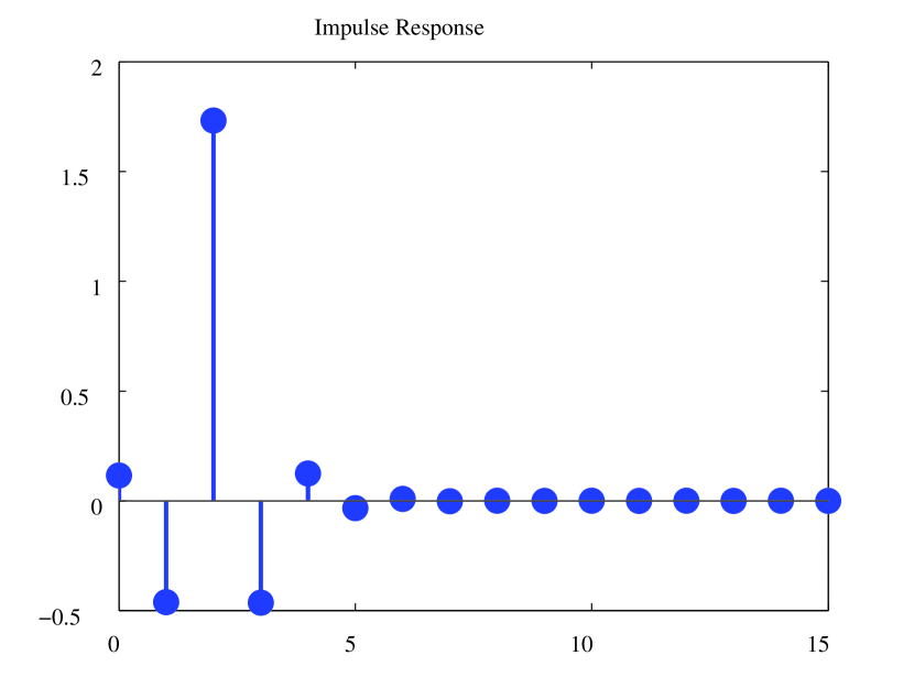
Figure 5. Impulse response of $H^{\infty}$ optimal IIR filter $\psi(z)$

For comparison, we also design a 5-tap FIR filter by the constrained least square design (CLSD) [18] and the Kaiser windowed approximation (KWA) [20]. Table 1 shows the coefficients of the $H^{\infty}$ optimal FIR filter, the filters by CLSD and by KWA.

Table 1. Coefficient $a_{k}$ of FIR filter $\psi(z)$

$k$	$H^{\infty}$ optimal	CLSD [18]	KWA [20]
0	0.1152359	0.0991561	0.06049527
1	-0.4614954	-0.4599156	-0.37739071
2	1.7307475	1.7215190	1.63379087
3	-0.4614951	-0.4599156	-0.37739071
4	0.1152352	0.0991561	0.06049527

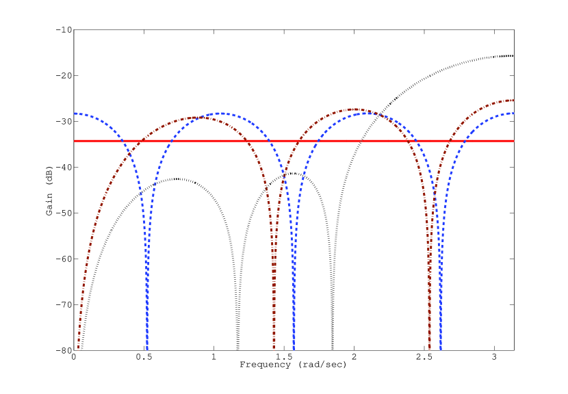
Figure 6. Magnitude plot of $E(z)$: $H^{\infty}$ optimal IIR (solid), $H^{\infty}$ optimal FIR (dash), CLSD [18] (dash-dots), and KWA [20] (dots).

Figure 6 shows the magnitude of the frequency response of the error system $E(z)=z^{-3}-\phi(z)\psi(z)$. From this figure, we see that the $H^{\infty}$ optimal IIR filter given by (14) has the allpass characteristic. The $H^{\infty}$ optimal FIR filter shows almost the same characteristic as the CLSD filter except at the zero frequency. This is because CLSD aims at exact inversion for DC signals. At the price of that, the CLSD filter exhibits larger errors in the high frequency range. The KWA filter shows the same nature. Table 2 shows the $H^{\infty}$ norm of the error system $E(z)$.

Table 2. $H^{\infty}$ norm of $E(z)$

Method	$\|E\|_{\infty}$	$\|E\|_{\infty}$ in dB
$H^{\infty}$ optimal IIR	0.019238	-34.3168
$H^{\infty}$ optimal FIR	0.038597	-28.2689
CLSD [18]	0.053446	-25.4417
KWA [20]	0.16348	-15.7307

By Figure 6 and Table 2, we can see that the $H^{\infty}$ optimal IIR filter is superior to CLSD by about 9 dB and KWA by about 19 dB at the worst case frequencies. In general, the purpose of $H^{\infty}$ design is to minimize the error in the worst case. This means that the $H^{\infty}$ design is against uncertainties in input signals, and this is an advantage of the $H^{\infty}$ design. While CLSD may perform better when the inputs can be predicted with certainty (e.g., the inputs are all DC signals), the $H^{\infty}$ design (worst case optimization) performs better when we do not have much information on the frequency characteristic of input signals. To see this robustness property of the $H^{\infty}$ method, we simulate spline interpolation by $H^{\infty}$ method and CLSD. The original analog signal is set to be the rectangular wave with the frequency 1 (rad/sec) filtered by the 8-th order Butterworth lowpass filter with the cut-off frequency 1.5 (rad/sec).

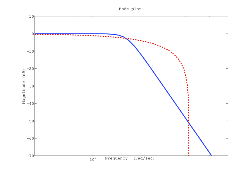
Figure 7. Bode magnitude plot of 8-th order Butterworth lowpass filter (solid) and weighting function $w(z)=(1+z^{-1})/2$.

Figure 7 shows the Bode magnitude plot of this lowpass filter, and Figure 8 shows the analog signal filtered by the Butterworth filter and its sampled-data. Note that this input signal is not exactly in the spline space $S_{N}$ defined in (1). This situation assumes that we have a priori knowledge on the input analog signal that the signal contains frequencies mostly in $[0,1.5]$ (rad/sec).

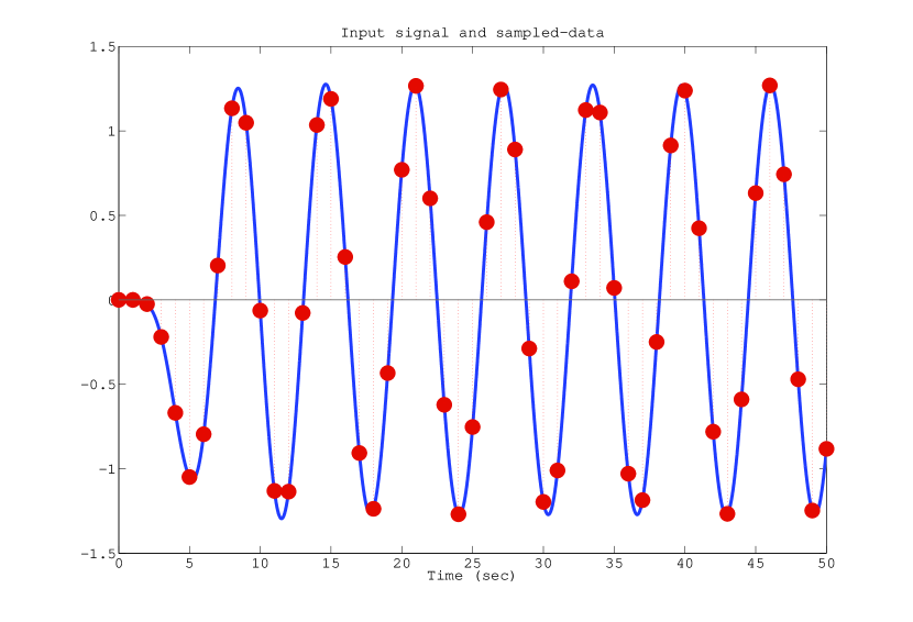
Figure 8. The original analog signal and its sampled-data

To bring this knowledge into our design, we adopt the following frequency weight:

$$w(z)=\frac{1}{2}(1+z^{-1}).$$

The Bode magnitude plot of $w(z)$ is shown in Figure 7. With this weight, we design 5-tap FIR filter by the LMI in Proposition 2. Figure 9 shows the reconstruction errors of the spline interpolation by this FIR filter, the $H^{\infty}$ optimal IIR filter given by (14), and the CLSD filter given in Table 1. Note that the errors in Figure 9 do not vanish at the sampling instants since the original signal $x(t)$ does not in the spline space $S_{N}$. The local minima in the errors are points at which the original signal and the reconstructed one cross. The $L^{2}$ norms of these errors are 1.9181 (CLSD), 1.2289 (unweighted $H^{\infty}$ optimal), and 0.7993 (weighted $H^{\infty}$ optimal). The weighted $H^{\infty}$ optimal FIR filter shows the best performance since this is designed with a priori knowledge on the signal frequency distribution. On the other hand, the CLSD filter is designed to achieve perfect fit for DC signals, but does not take other signals into account.

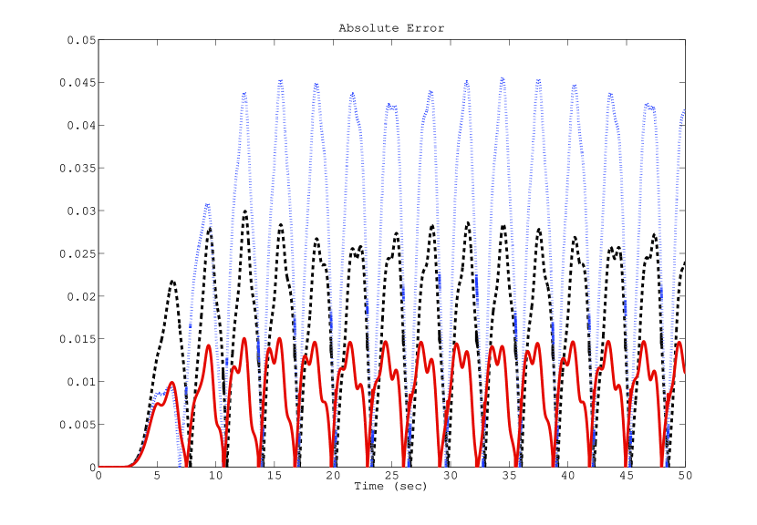
Figure 9. Reconstruction error by weighted $H^{\infty}$ optimal FIR (solid), unweighted $H^{\infty}$ optimal IIR (dash), and CLSD [18] (dots).

As a result it exhibits larger errors for unexpected signals as shown in Figure 6.

There is also a design method for causal spline interpolation, the maximum order minimum support (MOMS) function method by Blu et al. [3]. In contrast to the methods examined in this section, the MOMS method optimizes the base functions. To investigate robustness of the MOMS method by using the $H^{\infty}$ norm and to compare it with our method, the optimality should be measured in sampled-data $H^{\infty}$ norm [4]. This is a theme for future study.

6. Conclusion

In this paper, we have proposed a design of causal interpolation with polynomial splines. The design is formulated as an $H^{\infty}$ optimization problem. In the case of the cubic spline, the optimal solution is given in a closed form. Higher-order optimal filters can effectively be solved by using MATLAB. We have also shown that the $H^{\infty}$ optimal FIR filter can be designed by an LMI. A design example have been shown to illustrate the result.

A future topic is the $H^{\infty}$ design when $d$ is not an integer, and also the order of the spline is fractional [17]. This can be formulated by $H^{\infty}$ optimization for non-rational transfer functions (or infinite-dimensional systems).

References

- [1] L. Baboulaz and P. L. Dragotti, Exact feature extraction using finite rate of innovation principles with an application to image super-resolution, IEEE Trans. Image Processing, vol. 18, no. 2, pp. 281–298, 2009.
- [2] G. Balas, R. Chiang, A. Packard and M. Safonov, Robust Control Toolbox Version 3, The MathWorks, 2005.
- [3] T. Blu, P. Thévenaz and M. Unser, High-quality causal interpolation for online unidimensional signal processing, Proc. of the 12th EUSIPCO, pp. 1417–1420, 2004.
- [4] T. Chen and B. A. Francis, Optimal Sampled-Data Control Systems, Springer, 1995.
- [5] T. Chen and B. A. Francis, Design of multirate filter banks by optimization, IEEE Trans. Signal Processing, vol. 43, no. 12, pp. 2822–2830, 1995.
- [6] L. Demaret, N. Dyn, and A. Iske, Image compression by linear splines over adaptive triangulations, Signal Processing, vol. 86, pp. 1604–1616, 2006.
- [7] B. Hassibi, A. T. Erdogan, and T. Kailath, MIMO linear equalization with an criterion, IEEE Trans. Signal Processing, vol. 54, no. 2, pp. 499–511, 2006.
- [8] T. Hastie, R. Tibshirani, and J. Friedman, The Elements of Statistical Learning, Springer, 2001.
- [9] H. Hou and H. C. Andrews, Cubic splines for image interpolation and digital filtering, IEEE Trans. Acoust., Speech, Signal Processing, vol. 26, no. 6, pp. 508–517, 1978.
- [10] I. J. Schoenberg, On spline interpolation at all integer points of the real axis, Delange-Pisot-Poitou. Theorie des nombres, vol. 9, no. 1, pp. 1–18, 1967.
- [11] B. W. Silverman, Some aspects of the spline smoothing approach to non-parametric regression curve fitting, Journal of the Royal Statistical Society, Series B, vol. 47, no. 1, pp. 1–52, 1985.
- [12] G. Strang and T. Nguyen, Wavelets and Filter Banks, Wellesley-Cambridge Press, 1996.
- [13] M. Unser, Splines: A perfect fit for signal and image processing, IEEE Signal Processing Magazine, Vol. 16, No. 6, pp. 22–38, 1999.
- [14] M. Unser, Sampling — 50 years after Shannon, Proceedings of the IEEE, vol. 88, no. 4, pp. 569–587, 2000.
- [15] M. Unser, A. Aldroubi and M. Eden, B-Spline signal processing: Part-I — Theory, IEEE Trans. Signal Processing, vol. 41, no. 2, pp. 821–833, 1993.
- [16] M. Unser, A. Aldroubi and M. Eden, B-Spline signal processing: Part-II — Efficient design and applications, IEEE Trans. Signal Processing, vol. 41, no. 2, pp. 834–848, 1993.
- [17] M. Unser and T. Blu, Fractional splines and wavelets, SIAM Rev., vol. 42, no. 1, pp. 43–67, 2000.
- [18] M. Unser and M. Eden, FIR approximations of inverse filters and perfect reconstruction filter banks, Signal Processing, vol. 36, pp. 163–174, 1994.
- [19] M. Unser, P. Thévenaz, and L. Yaroslavsky, Convolution-based interpolation for fast, high-quality rotation of images, IEEE Trans. Image Processing, vol. 4, no. 10, pp. 1371–1381, 1995.
- [20] B. Vrcelj and P. P. Vaidyanathan, Efficient implementation of all-digital interpolation, IEEE Trans. Image Processing, vol. 10, no. 11, pp. 1639–1646, 2001.
- [21] J. L. Walsh, Interpolation and Approximation by Rational Functions in the Complex Domain, 5th ed., American Mathematical Society, 1969.
- [22] Y. Yamamoto, B. D. O. Anderson, M. Nagahara and Y. Koyanagi, Optimizing FIR approximation for discrete-time IIR filters, IEEE Signal Processing Lett., vol. 10, no. 9, pp. 273–276, 2003.
- [23] G. Zames, Feedback and optimal sensitivity: model reference transformations, multiplicative seminorms and approximate inverses, IEEE Trans. Autom. Control, vol. 26, pp. 301–320, 1981.
- [24] K. Zhou, J. C. Doyle and K. Glover, Robust and Optimal Control, Prentice Hall, 1995.
- [25] http://www-ics.acs.i.kyoto-u.ac.jp/∼nagahara/cs/