Precision Measurements of Temperature and Chemical Potential of Quantum Gases

Abstract

We investigate the sensitivity with which the temperature and the chemical potential characterizing quantum gases can be measured. We calculate the corresponding quantum Fisher information matrices for both fermionic and bosonic gases. For the latter, particular attention is devoted to the situation close to the Bose-Einstein condensation transition, which we examine not only for the standard scenario in three dimensions, but also for generalized condensation in lower dimensions, where the bosons condense in a subspace of Hilbert space instead of a unique ground state, as well as condensation at fixed volume or fixed pressure. We show that Bose Einstein condensation can lead to sub-shot noise sensitivity for the measurement of the chemical potential. We also examine the influence of interactions on the sensitivity in three different models, and show that mean-field and contact interactions deteriorate the sensitivity but only slightly for experimentally accessible weak interactions.

I Introduction

The use of gases for measurements of temperature and pressure has a long history, going back at least as far as Galileo Galilei in the 16th century, who built a thermoscope based on a glass pipe filled with air and sealed with a water surface. Variations in temperature show up as variations of the level of the water, as depending on the contraction of the air water gets sucked up to different levels Benedict84 . Still today, gas thermometry plays an important role for the calibration of other thermometers, even though a lot of effort has to be spent to compensate for many effects of real working substances Schooley90 . A high precision solid state thermometer for temperatures spanning four orders of magnitude based on the noise properties of an electron gas was developed by Spietz et al. Spietz03 . Shot-noise thermometry of an electron gas was also applied recently to quantum Hall edge states Levkivskyi and Sukhorukov (2012).

The chemical potential is, besides temperature, the only other independent parameter that characterizes ideal quantum gases, and one may legitimately ask how sensitively both parameters can be measured in principle. For charged gases, such as the electron gas responsible for electrical conductance in a metal or semi-conductor, the chemical potential is directly linked to voltage. More precisely, without current flow, the voltage drop between two parts of a sample is given by the difference between the chemical potentials divided by the electron charge, $V=(\mu_{2}-\mu_{1})/e$, such that the precision of a measurement of the chemical potential translates directly into the precision of voltage measurement Madelung08 . Voltage measurements on the other hand are at the basis of a huge variety of modern sensors, such that knowing the ultimate precision with which chemical potentials can be measured is of fundamental importance. For instance, voltage measurements can be employed in magnetometry in the presence of Hall effects or magnetoresistances, as an alternative to other metrological schemes Savukov2005 ; Fang2013 ; Loretz2013 ; Aiello2013 ; Steinke ; Eto ; Waxman ; Puentes .

Establishing the ultimate bounds on sensitivity of measurements is one of the major goals of parameter estimation theory. This theoretical frame work was developed in classical statistical analysis Cramér (1946), and later generalized to the quantum world Holevo ; Helstrom ; Braunstein and Caves (1994). It leads to the (quantum) Cramér-Rao bound that establishes that under suitable regularity conditions and for unbiased estimators the best sensitivity with which a parameter $x$ can be measured is given by the inverse of the (quantum) Fisher information. In classical statistical analysis, the classical Fisher information characterizes the probability distribution of the measurement results $A_{i}$ of the measured quantity $A$ (which may be different from $x$) given the parameter $x$. The corresponding bound is optimized over all estimator functions. In the quantum world, all statistical information is coded in the quantum state (density matrix) of the system characterized by the parameter $x$, and the quantum Cramér-Rao bound is obtained from the classical Cramér-Rao bound by additionally optimizing over all possible positive operator-valued measure (POVM) measurements. For unbiased estimators the bound is tight. As a result, it represents the best sensitivity with which a parameter can be measured, no matter what the measurement strategy, data analysis, feedback schemes etc.

In the quantum physics community interest has recently arisen in the question whether quantum mechanical effects may be used for enabling or improving temperature measurements Stace (2010); Ruostekoski et al. (2009); Sabin et al. (2013). In Stace (2010) it was shown that for any thermalizing thermometer with extensive internal energy the sensitivity scales as $1/\sqrt{N}$, corresponding to a linear scaling of the quantum Fisher information with $N$. This scaling is called shot-noise limit or standard quantum limit (SQL). On the other hand, it is well-known for the measurement of other quantities that using quantum effects one can beat in principle the SQL. Examples include the use of squeezed states Caves (1981) (which allow one to change the prefactor of the linear scaling of the quantum Fisher information with $N$, a strategy implemented in Advanced-LIGO), or entangled states Giovannetti et al. (2004, 2006, 2011), which can enable reaching the so-called Heisenberg limit (HL) characterized by a Fisher information that scales as $N^{2}$. A popular entangled state is the NOON state Boto et al. (2000). It was shown in Stace (2010) that the principles of interferometric quantum-enhanced metrology can be applied to the measurement of temperature, allowing one at least in principle to achieve HL scaling. In several other systems the sensitivity of quantum mechanical interference to thermal noise was already used for thermometry Brunelli et al. (2011); Slodi\vcka et al. (2012), but no attempts were made for establishing the ultimate sensitivity of such an approach.

Few experiments using entangled states have surpassed the SQL, and all experiments have been limited to small values of $N$, due to the extreme sensitivity of such states to decoherence. Indeed it has become clear that the smallest amount of Markovian decoherence leads back to the SQL Huelga et al. (1997); Kolodynski10 ; Escher2011 ; Alipour2013 , limiting the method to short time analyses Benatti2013-2 or niche applications Gross2010 ; Riedel2010 ; Wolfgramm et al. (2012). On the other hand, while an entangled state of distinguishable particles is needed for beating the SQL in interferometric metrology, a HL-like scaling can be reached by feeding interferometers with unentangled states of identical particles that cannot be distinguished by any degree of freedom Holland1993 ; Benatti2010 ; Benatti2011 ; Argentieri2011 ; Benatti2013 . Another strategy is the use of interactions between the $N$ particles Luis (2004, 2007); Napolitano et al. (2011). With $k$-body interactions one may even surpass the HL, but interactions between all particles are required, which makes such models unphysical for large particle numbers due to the resulting non-extensive character of the total energy. In Braun and Martin (2011) a method of “coherent averaging” was proposed for reaching the HL, in which the $N$ constituents interact with a common “quantum bus” which is then read out. The quantum bus can even be an environment of which one has no full control, leading to the possibility of using collective decoherence effects for precision measurements Braun and Martin .

In the present paper, we shall discuss the scaling of the Fisher matrix characterizing measurements of both temperature and chemical potential of ideal quantum gases with the average number of particles, as well as of three different models of interacting particles, which will establish the ultimate sensitivity with which these parameters can be measured. We pay particular attention to the influence of the Bose-Einstein condensation (BEC) phase transition in bosonic gases. Indeed, it is well known that phase transitions can lead to enhanced susceptibilities, as is witnessed by large fluctuations Huang , and, closely related, to large quantum Fisher information. Discontinuities in the quantum Fisher information were proposed before as a tool for detecting phase transitions in the absence of knowledge of an order parameter Zanardi06 . We will see that indeed the onset of BEC can improve the sensitivity of a measurement of the chemical potential beyond the shot-noise limit. We carefully analyse several scenarios of BEC: the standard case of fixed density in the thermodynamic limit, the case of cooling at fixed volume, the case of isobaric cooling, as well as generalized BEC in lower dimensions, where condensation occurs in a subspace of Hilbert space, instead of only the ground state. We also examine the influence of interactions on the sensititivy in the framework of three different models, and show that interactions can be detrimental for the sensitivity with which the chemical potential can be measured.

The paper is organized as follows. In sections II and III preliminary discussions respectively on quantum metrology and quantum gases are presented. Our results, based on these preliminary notions, are reported in section IV for gases in the continuum approximation, in section V for BEC, and in section VI for bosonic interactiong gases. Conclusions are discussed in section VII, and some technical details in the appendices.

II Metrology with quantum gases

We start by introducing the formalism of parameter estimation in the context of quantum gases. Consider the hamiltonian $H$ and the total number of particles is described by the operator

$$N=\sum_{k}a_{k}^{\dagger}a_{k},$$ (1)

where $a_{k}^{\dagger}$ and $a_{k}$ are the creation and annihilation operators of the $k$-th mode. In condensed matter systems, the hamiltonian and the total number of particles commute with each other, and the common eigenvectors are $|N,E_{N}\rangle$ with particle number eigenvalues $N$ and hamiltonian eigenvalues $E_{N}$. The grand canonical thermal state is

$$\rho_{\beta,\mu}=\frac{e^{-\beta(H-\mu N)}}{Z_{G}}=\sum_{N,E_{N}}\rho_{\beta,\mu}^{(N,E_{N})}|N,E_{N}\rangle\langle N,E_{N}|,\qquad\rho_{\beta,\mu}^{(N,E_{N})}=\frac{e^{-\beta(E_{N}-\mu N)}}{Z_{G}}$$ (2)

where we have defined the grand canonical partition function $Z_{G}=\sum_{N,E_{N}}\rho_{\beta,\mu}^{(N,E_{N})}$.

In statistical mechanics, the inverse temperature $\beta$ and the chemical potential $\mu$ are the Lagrange multipliers of the average energy and the average total number of particle respectively. These two latter quantities fix $(\beta,\mu)$. Therefore, one way of estimating $(\beta,\mu)$ is through measuring the average energy and the number of particles. We will discuss how this is related to the best sensitivity for the estimation of $(\beta,\mu)$.

Quantum estimation theory Helstrom ; Holevo provides a bound for the covariance matrix of the parameter estimators. The ingredients are the symmetric logarithmic derivatives with respect to the parameters $\lambda_{1}=\beta$, $\lambda_{2}=\mu$

$$L_{\lambda_{j}}=\sum_{N,E_{N}}\frac{\partial_{\lambda_{j}}\rho_{\beta,\mu}^{(N,E_{N})}}{\rho_{\beta,\mu}^{(N,E_{N})}}|N,E_{N}\rangle\langle N,E_{N}|=\begin{cases}\mu N-H-\langle\mu N-H\rangle&\mbox{if }j=1\\ \beta\left(N-\langle N\rangle\right)&\mbox{if }j=2\end{cases},$$ (3)

and the quantum Fisher matrix has entries

$$F_{\lambda_{j},\lambda_{l}}=\frac{1}{2}{\rm tr}\left(\rho\{L_{\lambda_{j}},L_{\lambda_{l}}\}\right)=\sum_{N,E_{N}}\frac{(\partial_{\lambda_{j}}\rho_{\beta,\mu}^{(N,E_{N})})(\partial_{\lambda_{l}}\rho_{\beta,\mu}^{(N,E_{N})})}{\rho_{\beta,\mu}^{(N,E_{N})}}.$$ (4)

where $\{,\}$ denotes the anti commutator. The covariance matrix of any estimator of $\lambda$ is bounded by the quantum Cramér-Rao bound,

$$\begin{pmatrix}\displaystyle{\rm var}(\beta)&{\rm cov}(\beta,\mu)\\ \displaystyle{\rm cov}(\beta,\mu)&{\rm var}(\mu)\end{pmatrix}\geqslant F^{-1}=\begin{pmatrix}\displaystyle\frac{F_{\mu,\mu}}{F_{\mu,\mu}F_{\beta,\beta}-F_{\mu,\beta}^{2}}&\displaystyle\frac{F_{\mu,\beta}}{F_{\mu,\beta}^{2}-F_{\mu,\mu}F_{\beta,\beta}}\\ \displaystyle\frac{F_{\mu,\beta}}{F_{\mu,\beta}^{2}-F_{\mu,\mu}F_{\beta,\beta}}&\displaystyle\frac{F_{\beta,\beta}}{F_{\mu,\mu}F_{\beta,\beta}-F_{\mu,\beta}^{2}}\end{pmatrix},$$ (5)

where ${\rm var}$ and ${\rm cov}$ are the variances and the covariance of the estimation problem, and $A\geqslant B$ means that $A-B$ is a semi-positive definite matrix.

If one parameter, say $\beta$ ($\mu$), is known the inverse of the diagonal entry $F_{\mu,\mu}$ ($F_{\beta,\beta}$) is the best sensitivity for the estimation of $\mu$ ($\beta$). A non-diagonal Fisher matrix, i.e. $F_{\mu,\beta}\neq 0$, means that estimation of $\beta$ and $\mu$ are correlated. Thus, the diagonal entries of the inverse Fisher matrix $F^{-1}$ are the optimal sensitivities of each parameter in a joint measurement, and the off-diagonal term is the corresponding covariance.

Denoting with $\Delta^{2}$ and ${\rm Cov}$ respectively the variance and the covariance in the grand canonical state, the Fisher matrix explicitly reads

$$F_{\mu,\mu}=\beta^{2}\Delta^{2}N,$$ (6)

$$F_{\beta,\beta}=\Delta^{2}(\mu N-H),$$ (7)

$$F_{\mu,\beta}=F_{\beta,\mu}=\beta\,{\rm Cov}(N,\mu N-H),$$ (8)

The latter equations can be computed by the standard relations

$$\Delta^{2}N=\frac{1}{\beta^{2}}\frac{\partial^{2}}{\partial\mu^{2}}\ln Z_{G}=\frac{1}{\beta}\frac{\partial}{\partial\mu}\langle N\rangle,$$ (9)

$$\Delta^{2}(\mu N-H)=\frac{\partial^{2}}{\partial\beta^{2}}\ln Z_{G}=\frac{\partial}{\partial\beta}\langle\mu N-H\rangle,$$ (10)

$${\rm Cov}(N,\nu N-H)=\frac{\partial}{\partial\beta}\frac{1}{\beta}\frac{\partial}{\partial\mu}\ln Z_{G}=\frac{\partial}{\partial\beta}\langle N\rangle,$$ (11)

The optimal measurement is a projective measurement onto the eigenstates of its symmetric logarithmic derivatives Helstrom ; Holevo . For the grand canonical thermal states considered here, the symmetric logarithmic derivatives commute with each other. Hence, the two parameters can be simultaneously measured, contrary to the general case of multivariate quantum metrology. Our problem is a very special case of quantum estimation where only the eigenvalues of the state depend on the parameters $(\beta,\mu)$, and the estimation problem becomes a classical problem in the representation of the Fock basis (31).

For a temperature measurement which is known to be difficult, different approaches have been proposed. One is based on the measurement of a spin gradient between two domains of a spin mixture separated by a magnetic field gradient Weld2009 . In Leanhardt2013 , where a temperature of 500 $p$K was reached, temperature was calibrated to the BEC transition temperature by measuring trap frequency and average particle number. Zhou and Ho proposed the use of local particle number fluctuations which are related to temperature through a generalized dissipation fluctuation theorem Zhou2011 . Temperature measurements based on fluctuations of the total particle number were realized in Muller2010 ; Sanner2010 . Our results show that the measurement of the particle number fluctuations is optimal for the estimation of chemical potential. Particle counting has been implemented for fermionic Muller2010 ; Sanner2010 and bosonic Greiner2001 ; Esteve2006 ; Bouchoule2011 ; Armijo2011 gases, but, up to our knowledge, measurement of the chemical potential based on this technique has not been implemented yet.

Some general remarks are in order. The variance of the number of particles is directly connected to the thermodynamic stability, through the isothermal compressibility $\kappa_{T}$ Huang , which measures how the system responds to variations of the pressure:

$$\kappa_{T}=-\frac{1}{V}\left(\frac{\partial V}{\partial P}\right)_{T}=\frac{\beta\Delta^{2}N}{\varrho\,\langle N\rangle}.$$ (12)

Hence, any superlinear scaling of the Fisher information $F_{\mu,\mu}$ implies thermodynamical instability via (6), i.e. the compressibility grows with the number of particles, diverges in the thermodynamic limit Huang , and ceases to be an intensive quantity. The thermodynamic instability of superlinear particle number fluctuations in the grand canonical state has been used for claiming that the inappropriate application of the grand canonical ensemble may give rise to unphysical results Yukalov2005 . But the grand canonical thermal is a physically meaningful state for the following reasons: Firstly, the grand canonical state naturally arises as the equilibrium state when particles can be exchanged with the thermal bath Huang ; Reichl . Secondly, it has been argued that the unique correct definition of the chemical potential for finite systems is provided by the grand canonical state, even if there are other inequivalent definitions converging to the same quantity in the thermodynamic limit Kaplan2006 . Finally, superlinear fluctuations can be stabilized and observed within mesoscopic sizes Greiner2001 ; Esteve2006 ; Bouchoule2011 ; Armijo2011 . For these reasons we will base our analysis on the grand-canonical ensemble.

II.1 Optimal measurements

We now derive the joint measurement of the chemical potential and the inverse temperature that attains the quantum Cramér-Rao bound (5). As we mentioned, the two symmetric logarithmic derivatives commute with each other. This allows the unusual situation where the two parameters $(\beta,\mu)$ can be measured simultaneously. In this case, applying the transformation which diagonalizes the matrix $F^{-1}$ to the inequality (5), we find two uncorrelated estimations, i.e. with vanishing covariance, of linear combinations of the parameters $(\beta,\mu)$. At this aim, it is convenient to consider dimensionless parameters which can be summed without issues about physical dimensions. The dimensionless parameters are $(\bar{\beta}=\beta/\beta_{0},\bar{\mu}=\mu/\mu_{0})$, where $\beta_{0}$ and $\mu_{0}$ are constant values. Examples for the case of fixed volume are $\mu_{0}=\beta_{0}^{-1}=2\pi^{2}\hslash^{2}/(mV_{d}^{2/d})$ for homogeneous gases and $\mu_{0}=\beta_{0}^{-1}=\hslash\Omega_{d}$ for harmonically trapped gases; if the density is fixed, one can choose $\mu_{0}=\beta_{0}^{-1}=2\pi^{2}\hslash^{2}\rho^{2/d}/m$ for homogeneous gases and $\mu_{0}=\beta_{0}^{-1}=\hslash\tilde{\rho}^{1/d}$ for harmonically trapped gases. The quantum Cramér-Rao bound for the dimensionless parameters is

$$\begin{pmatrix}\displaystyle{\rm var}(\bar{\beta})&{\rm cov}(\bar{\beta},\bar{\mu})\\ \displaystyle{\rm cov}(\bar{\beta},\bar{\mu})&{\rm var}(\bar{\mu})\end{pmatrix}\geqslant\begin{pmatrix}\displaystyle\frac{F_{\bar{\mu},\bar{\mu}}}{F_{\bar{\mu},\bar{\mu}}F_{\bar{\beta},\bar{\beta}}-F_{\bar{\mu},\bar{\beta}}^{2}}&\displaystyle\frac{F_{\bar{\mu},\bar{\beta}}}{F_{\bar{\mu},\bar{\beta}}^{2}-F_{\bar{\mu},\bar{\mu}}F_{\bar{\beta},\bar{\beta}}}\\ \displaystyle\frac{F_{\bar{\mu},\bar{\beta}}}{F_{\bar{\mu},\bar{\beta}}^{2}-F_{\bar{\mu},\bar{\mu}}F_{\bar{\beta},\bar{\beta}}}&\displaystyle\frac{F_{\bar{\beta},\bar{\beta}}}{F_{\bar{\mu},\bar{\mu}}F_{\bar{\beta},\bar{\beta}}-F_{\bar{\mu},\bar{\beta}}^{2}}\end{pmatrix},$$ (13)

with

$$F_{\bar{\beta},\bar{\beta}}=\beta_{0}^{2}F_{\beta,\beta},\qquad F_{\bar{\mu},\bar{\mu}}=\mu_{0}^{2}F_{\mu,\mu},\qquad F_{\bar{\beta},\bar{\mu}}=\beta_{0}\mu_{0}F_{\beta,\mu}.$$ (14)

The right-hand-side of the inequality (13) is diagonalized by the following orthogonal matrix

$$R=\begin{pmatrix}\displaystyle\frac{F_{\bar{\beta},\bar{\beta}}-F_{\bar{\mu},\bar{\mu}}-\sqrt{4F_{\bar{\beta},\bar{\mu}}^{2}+(F_{\bar{\beta},\bar{\beta}}-F_{\bar{\mu},\bar{\mu}})^{2}}}{\sqrt{4F_{\bar{\beta},\bar{\mu}}^{2}+\left(F_{\bar{\beta},\bar{\beta}}-F_{\bar{\mu},\bar{\mu}}-\sqrt{4F_{\bar{\beta},\bar{\mu}}^{2}+(F_{\bar{\beta},\bar{\beta}}-F_{\bar{\mu},\bar{\mu}})^{2}}\right)^{2}}}&\displaystyle\frac{2F_{\bar{\beta},\bar{\mu}}}{\sqrt{4F_{\bar{\beta},\bar{\mu}}^{2}+\left(F_{\bar{\beta},\bar{\beta}}-F_{\bar{\mu},\bar{\mu}}-\sqrt{4F_{\bar{\beta},\bar{\mu}}^{2}+(F_{\bar{\beta},\bar{\beta}}-F_{\bar{\mu},\bar{\mu}})^{2}}\right)^{2}}}\\ \displaystyle\frac{F_{\bar{\beta},\bar{\beta}}-F_{\bar{\mu},\bar{\mu}}+\sqrt{4F_{\bar{\beta},\bar{\mu}}^{2}+(F_{\bar{\mu},\bar{\mu}}-F_{\bar{\beta},\bar{\beta}})^{2}}}{\sqrt{4F_{\bar{\beta},\bar{\mu}}^{2}+\left(F_{\bar{\beta},\bar{\beta}}-F_{\bar{\mu},\bar{\mu}}+\sqrt{4F_{\bar{\beta},\bar{\mu}}^{2}+(F_{\bar{\beta},\bar{\beta}}-F_{\bar{\mu},\bar{\mu}})^{2}}\right)^{2}}}&\displaystyle\frac{2F_{\bar{\beta},\bar{\mu}}}{\sqrt{4F_{\bar{\beta},\bar{\mu}}^{2}+\left(F_{\bar{\beta},\bar{\beta}}-F_{\bar{\mu},\bar{\mu}}+\sqrt{4F_{\bar{\beta},\bar{\mu}}^{2}+(F_{\bar{\beta},\bar{\beta}}-F_{\bar{\mu},\bar{\mu}})^{2}}\right)^{2}}}\\ \end{pmatrix}.$$ (15)

The quantum Cramér-Rao bound (13) is then transformed into

$$\begin{pmatrix}\displaystyle{\rm var}(\bar{\lambda}_{1})&{\rm cov}(\bar{\lambda}_{1},\bar{\lambda}_{2})\\ \displaystyle{\rm cov}(\bar{\lambda}_{1},\bar{\lambda}_{2})&{\rm var}(\bar{\lambda}_{2})\end{pmatrix}=R\begin{pmatrix}\displaystyle{\rm var}(\bar{\beta})&{\rm cov}(\bar{\beta},\bar{\mu})\\ \displaystyle{\rm cov}(\bar{\beta},\bar{\mu})&{\rm var}(\bar{\mu})\end{pmatrix}R^{T}\geqslant\begin{pmatrix}\displaystyle F_{\bar{\lambda}_{1}}^{-1}&0\\ 0&\displaystyle F_{\bar{\lambda}_{2}}^{-1}\end{pmatrix},$$

with

$$\begin{pmatrix}\displaystyle\bar{\lambda}_{1}\\ \displaystyle\bar{\lambda}_{2}\end{pmatrix}=R\begin{pmatrix}\displaystyle\bar{\beta}\\ \displaystyle\bar{\mu}\end{pmatrix},\qquad F_{\bar{\lambda}_{j}}=\frac{1}{2}\left(F_{\bar{\beta},\bar{\beta}}+F_{\bar{\mu},\bar{\mu}}+(-1)^{j}\sqrt{4F_{\bar{\beta},\bar{\mu}}^{2}+(F_{\bar{\beta},\bar{\beta}}-F_{\bar{\mu},\bar{\mu}})^{2}}\right).$$ (16)

The symmetric logarithmic derivatives with respect to the parameters $\bar{\lambda}_{1,2}$ are

$$L_{\bar{\lambda}_{j}}=\sum_{N,E_{N}}\frac{\partial_{\bar{\lambda}_{j}}\rho_{\beta,\mu}^{(N,E_{N})}}{\rho_{\beta,\mu}^{(N,E_{N})}}|N,E_{N}\rangle\langle N,E_{N}|,$$ (17)

and explicitely

$$\begin{pmatrix}L_{\bar{\lambda}_{1}}\\ L_{\bar{\lambda}_{2}}\end{pmatrix}=R\begin{pmatrix}\beta_{0}&0\\ 0&\mu_{0}\end{pmatrix}\begin{pmatrix}L_{\beta}\\ L_{\mu}\end{pmatrix}=R\begin{pmatrix}\beta_{0}&0\\ 0&\mu_{0}\end{pmatrix}\begin{pmatrix}\mu N-H-\langle\mu N-H\rangle\\ \beta\left(N-\langle N\rangle\right)\end{pmatrix}.$$ (18)

According to quantum estimation theory Holevo ; Helstrom , the optimal estimation is then given by measuring the following observables

$$\begin{pmatrix}O_{\bar{\lambda}_{1}}\\ O_{\bar{\lambda}_{2}}\end{pmatrix}=\begin{pmatrix}\displaystyle\bar{\lambda}_{1}\mathbb{1}+\frac{L_{\bar{\lambda}_{1}}}{F_{\bar{\lambda}_{1}}}\\ \displaystyle\bar{\lambda}_{2}\mathbb{1}+\frac{L_{\bar{\lambda}_{2}}}{F_{\bar{\lambda}_{2}}}\end{pmatrix}=R\begin{pmatrix}\beta_{0}&0\\ 0&\mu_{0}\end{pmatrix}\begin{pmatrix}\displaystyle\frac{\beta}{\beta_{0}^{2}}\mathbb{1}+\frac{\mu N-H-\langle\mu N-H\rangle}{F_{\bar{\lambda}_{1}}}\\ \displaystyle\frac{\mu}{\mu_{0}^{2}}\mathbb{1}+\frac{\beta\left(N-\langle N\rangle\right)}{F_{\bar{\lambda}_{2}}}\end{pmatrix}.$$ (19)

For the single parameter estimation of $\beta$ or $\mu$, when the other parameter in known, the optimal estimations are given respectively by the measurement of following observables

$$O_{\beta} = \beta\mathbb{1}+\frac{L_{\beta}}{F_{\beta,\beta}}=\beta\mathbb{1}+\frac{\mu N-H-\langle\mu N-H\rangle}{\Delta^{2}(\mu N-H)},$$ (20)

$$O_{\mu} = \mu\mathbb{1}+\frac{L_{\mu}}{F_{\mu,\mu}}=\mu\mathbb{1}+\frac{N-\langle N\rangle}{\beta\Delta^{2}N}.$$ (21)

It is straightforwad to show that the above estimators are unbiased and attain the quantum Cramér-Rao bound (II.1):

$$\langle O_{\bar{\lambda}_{j}}\rangle=\bar{\lambda}_{j},\qquad\Delta^{2}O_{\bar{\lambda}_{j}}=\frac{1}{F_{\bar{\lambda}_{j}}},\qquad{\rm Cov}(O_{\bar{\lambda}_{1}},O_{\bar{\lambda}_{2}})=0,$$ (22)

$$\langle O_{\beta}\rangle=\beta,\qquad\Delta^{2}O_{\beta}=\frac{1}{F_{\beta,\beta}},$$ (23)

$$\langle O_{\mu}\rangle=\mu,\qquad\Delta^{2}O_{\mu}=\frac{1}{F_{\mu,\mu}}.$$ (24)

This optimal joint estimation can be realized e.g. by measuring the energy and the number of particles. In general, in quantum parameter estimation the optimal measurement depends of the parameters to be estimated, and thus is called local estimation. Interestingly, the optimal sensitivities for single parameter estimation of $\mu$ and $\beta$, when the other parameter is known, are achieved by a global estimation, in the sense that the optimal measurement can be implemented with an operator that does not depend on the parameter to be estimated. The optimal estimators themself do depend on the parameters to be estimated, but that prior knowledge is only needed on the level of the data analysis, not for the choice of the measurement itself. This unusual situation is reminiscent once more of the situation in classical estimation theory, where the measurement is fixed from the beginning, and can be tracked back to the exponential form of the density matrix as function of $\beta(H-\mu N)$, which makes that the logarithmic derivatives only depend on these operators, but not anymore on the corresponding parameter.

Another joint optimal estimation can be derived from the consideration that our estimation problem reduces to a classical problem in the joint eigenbasis of $H$ and of $N$. Consequently, the quantum Fisher information is the classical Fisher information of the probability distribution $\rho_{\beta,\mu}^{(N,E_{N})}$. It is known that the maximum likelihood estimator is asymptotically biased and optimal, in the sense of achieving the classical Cramér-Rao bound, in the limit of infinitely many measurements Helstrom ; Holevo . The Cramér-Rao bound for $M$ measurements reads

$$\begin{pmatrix}\displaystyle{\rm var}(\beta)&{\rm cov}(\beta,\mu)\\ \displaystyle{\rm cov}(\beta,\mu)&{\rm var}(\mu)\end{pmatrix}\geqslant(MF)^{-1}.$$ (25)

Consider the outcomes of particle number and energy measurements $\{N^{(i)},E^{(i)}_{N^{(i)}}\}_{i=1,\dots,M}$. The maximum likelihood esestimation consists in maximizing the average logarithmic likelihood ${\cal L}=\frac{1}{M}\ln\prod_{i}\rho_{\beta,\mu}^{(N^{(i)},E^{(i)}_{N^{(i)}})}$ with respect to the parameters to be estimated. This maximization problem is equivalent to impose vanishing derivatives

$$\begin{cases}\displaystyle\frac{\partial{\cal L}}{\partial\beta}=\frac{1}{M}\sum_{i=1}^{M}\left(\mu N^{(i)}-E^{(j)}_{N^{(i)}}\right)-\langle\mu N-H\rangle=0,\\ \displaystyle\frac{\partial{\cal L}}{\partial\mu}=\frac{\beta}{M}\sum_{i=1}^{M}N^{(i)}-\beta\langle N\rangle=0,\end{cases}$$ (26)

provided a negative Hessian matrix

$$\left.\begin{pmatrix}\displaystyle\frac{\partial^{2}{\cal L}}{\partial\beta^{2}}&\displaystyle\frac{\partial^{2}{\cal L}}{\partial\beta\partial\mu}\\ \displaystyle\frac{\partial^{2}{\cal L}}{\partial\beta\partial\mu}&\displaystyle\frac{\partial^{2}{\cal L}}{\partial\mu^{2}}\end{pmatrix}\right|_{\frac{\partial{\cal L}}{\partial\beta}=0,\frac{\partial{\cal L}}{\partial\mu}=0}=\begin{pmatrix}F_{\beta,\beta}&F_{\beta,\mu}\\ F_{\beta,\mu}&F_{\mu,\mu}\end{pmatrix}.$$ (27)

Equations (26) imply that the maximum likelihood estimator consists in finding the parameters $(\beta,\mu)$ for which the experimental averages $\frac{1}{M}\sum_{i=1}^{M}N^{(i)}$ and $\frac{1}{M}\sum_{i=1}^{M}E^{(i)}_{N^{(i)}}$ equal the theoretical quantities $\langle N\rangle$ and $\langle H\rangle$ respectively. The advantage of this estimator is that it does not require the a priori knowledge of the parameters $(\beta,\mu)$ even in the data analysis, although this property as well as the optimality hold true only in the limit $M\to\infty$.

Interestingly, the maximum likelihood estimator of single parameters, e.g. inverting $\frac{1}{M}\sum_{i=1}^{M}(\mu N^{(i)}-E^{(i)}_{N^{(i)}})=\langle\mu N-H\rangle$ for $\beta$ or $\frac{1}{M}\sum_{i=1}^{M}N^{(i)}=\langle N\rangle$ for $\mu$, achieves the Cramér-Rao bound (25) for any finite $M$. Indeed, $\langle N\rangle$ and $\langle\mu N-H\rangle$ are estimated from a finite sample of i.i.d. couples $(N^{(i)},E^{(i)}_{N^{(i)}})$ by $\frac{1}{M}\sum_{i=1}^{M}N^{(i)}$ and $\frac{1}{M}\sum_{i=1}^{M}(\mu N^{(i)}-E^{(i)}_{N^{(i)}})$ with standard deviations $\langle(\frac{1}{M}\sum_{i=1}^{M}N^{(i)}-\langle N\rangle)^{2}\rangle=\frac{1}{M}\Delta^{2}N$ and $\langle(\frac{1}{M}\sum_{i=1}^{M}(\mu N^{(i)}-E^{(i)}_{N^{(i)}})-\langle\mu N-H\rangle)^{2}\rangle=\frac{1}{M}\Delta^{2}(\mu-H)$ respectively. The variance of the estimation of $\mu$ ($\beta$) can be computed through simple laws of error propagation from the measurement of $\langle N\rangle$ ($\langle\mu N-H\rangle$):

$${\rm var}(\mu) = \left(\frac{\partial\mu}{\partial\langle N\rangle}\right)^{2}\frac{\Delta^{2}N}{M}=\frac{1}{M\beta^{2}\Delta^{2}N},$$ (28)

$${\rm var}(\beta) = \left(\frac{\partial\beta}{\partial\langle\mu N-H\rangle}\right)^{2}\frac{\Delta^{2}(\mu N-H)}{M}=\frac{1}{M\Delta^{2}(\mu N-H)}.$$ (29)

II.2 Ideal gases

We now focus on ideal gases of fermions or bosons. The hamiltonian in second quantization is

$$H=\sum_{k}\varepsilon_{k}a_{k}^{\dagger}a_{k},$$ (30)

where $\varepsilon_{k}$ is the energy of a single particle filling the $k$-th mode. The eigenvectors of both the hamiltonian and the total number of particles are the following Fock states

$$|\{n_{k}\}\rangle=\prod_{k}\frac{(a_{k}^{\dagger})^{n_{k}}}{\sqrt{n_{k}!}}|0\rangle=\bigotimes_{k}|n_{k}\rangle,$$ (31)

where $|0\rangle=\bigotimes_{k}|0_{k}\rangle$ is the vacuum, and we have used the tensor decomposition in terms of the single mode Fock states $|n_{k}\rangle=(a_{k}^{\dagger})^{n_{k}}/\sqrt{n_{k}!}|0_{k}\rangle$. The grand canonical thermal state is

$$\rho_{\beta,\mu}=\frac{e^{-\beta(H-\mu N)}}{Z_{G}}=\bigotimes_{k}\sum_{n_{k}}\rho_{\beta,\mu}^{(n_{k})}|n_{k}\rangle\langle n_{k}|,\qquad\rho_{\beta,\mu}^{(n_{k})}=\frac{e^{-\beta n_{k}(\varepsilon_{k}-\mu)}}{Z_{k}}$$ (32)

where we have defined the grand canonical partition function $Z_{G}=\prod_{k}Z_{k}$

$$Z_{k}=\begin{cases}1+e^{-\beta(\varepsilon_{k}-\mu)}&\mbox{for fermions}\\ \displaystyle\frac{1}{1-e^{-\beta(\varepsilon_{k}-\mu)}}&\mbox{for bosons}\end{cases}.$$ (33)

The sums over $n_{k}$ run from zero to one for fermions and from zero to infinity for bosons.

The average total number of particles and the average energy are, respectively,

$$\langle N\rangle=\sum_{k}\frac{1}{e^{\beta(\varepsilon_{k}-\mu)}\pm 1},$$ (34)

$$\langle H\rangle=\sum_{k}\frac{\varepsilon_{k}}{e^{\beta(\varepsilon_{k}-\mu)}\pm 1},$$ (35)

where the plus signs hold for fermions and the minus signs for bosons.

The symmetric logarithmic derivatives with respect to the parameters $\lambda_{1}=\beta$, $\lambda_{2}=\mu$ are

$$L_{\lambda_{j}}=\bigotimes_{k}\sum_{n_{k}}\left(\sum_{k^{\prime}}\frac{\partial_{\lambda_{j}}\rho_{\beta,\mu}^{(n_{k^{\prime}})}}{\rho_{\beta,\mu}^{(n_{k^{\prime}})}}\right)|n_{k}\rangle\langle n_{k}|=\begin{cases}\mu N-H-\langle\mu N-H\rangle&\mbox{if }j=1\\ \beta\left(N-\langle N\rangle\right)&\mbox{if }j=2\end{cases},$$ (36)

and the quantum Fisher matrix $F=[F_{\lambda_{j},\lambda_{l}}]$ with entries

$$F_{\lambda_{j},\lambda_{l}}=\frac{1}{2}{\rm tr}\left(\rho\{L_{\lambda_{j}},L_{\lambda_{l}}\}\right)=\sum_{k}\sum_{n_{k}}\frac{(\partial_{\lambda_{j}}\rho_{\beta,\mu}^{(n_{k})})(\partial_{\lambda_{l}}\rho_{\beta,\mu}^{(n_{k})})}{\rho_{\beta,\mu}^{(n_{k})}},$$ (37)

namely

$$F_{\mu,\mu}=\beta^{2}\Delta^{2}N=\beta^{2}\sum_{k}\frac{e^{\beta(\varepsilon_{k}-\mu)}}{(e^{\beta(\varepsilon_{k}-\mu)}\pm 1)^{2}},$$ (38)

$$F_{\beta,\beta}=\Delta^{2}(\mu N-H)=\sum_{k}(\mu-\varepsilon_{k})^{2}\frac{e^{\beta(\varepsilon_{k}-\mu)}}{(e^{\beta(\varepsilon_{k}-\mu)}\pm 1)^{2}},$$ (39)

$$F_{\mu,\beta}=F_{\beta,\mu}=\beta\,{\rm Cov}(N,\mu N-H)=\beta\sum_{k}(\mu-\varepsilon_{k})\frac{e^{\beta(\varepsilon_{k}-\mu)}}{(e^{\beta(\varepsilon_{k}-\mu)}\pm 1)^{2}},$$ (40)

where the plus signs hold for fermions and the minus signs hold for bosons.

The tensor product in the grand canonical state (32), the tensor product in the symmetric logarithmic derivatives (36), and the sum over the modes in the entries of the Fisher matrix (37) witness the lack of correlations in the mode representation Zanardi2001 ; Narnhofer2004 ; Barnum2004 ; Barnum2005 ; Benatti2012-1 ; Benatti2012-2 . The estimation of $(\beta,\mu)$ looks like a classical problem, but the classical scaling of the Fisher information may no longer hold, because the number of particles is not fixed. For instance, since the state (32) is separable with respect to the modes, standard arguments imply that the Fisher information scales linearly with the number of modes, as the sum in (37) suggests. However, this scaling does not correspond to a linear scaling in the average number of particles. Indeed, the state (32) is not in the convex hull of products of single-particle density matrices, because of the symmetrization or anti-symmetrization of the Hilbert space. Therefore, the estimation of $(\beta,\mu)$ with ideal quantum gases can be viewed as an abstract classical estimation problem with a fluctuating number of particles. We will show that this estimation is characterized by superlinear scalings of the Fisher matrix, which cannot result from the same estimation performed with classical gases.

III Bosonic and fermionic gases

In this section, we present the basic physical quantities of quantum gases, that will be employed later in the discussion of estimating $(\beta,\mu)$ within several settings. We focus on non-condensed bosonic and fermionic ideal gases in $d$ dimensions spatially confined ($=1,2,3$) either by a box with flat potential and periodic boundary conditions or by a harmonic potential. Bose-Einstein condensation shall be discussed in section V.

III.1 Homogeneous ideal gases

Homogeneous ideal gases in $d$ ($=1,2,3$) dimensions are confined in a parallelepiped shaped box of volume $V_{d}$, where $V_{1}=L_{x}$, $V_{2}=L_{x}L_{y}$, and $V_{3}=L_{x}L_{y}L_{z}$ with periodic boundary conditions. The single particle energies are $\varepsilon_{k}=(k_{x}^{2}+k_{y}^{2}+k_{z}^{2})/(2m)$ with $k_{x,y,z}=\frac{2\pi\hslash}{L_{x,y,z}}n_{x,y,z}$, and $n_{x,y,z}$ running over all the integers. In the limit of large volume $L_{x,y,z}\to\infty$, the vector $\mathbf{k}$ is approximated by a continuous variable $\mathbf{p}$, and the sum over the modes by an integral

$$\sum_{\mathbf{k}}=\frac{V_{d}}{(2\pi\hslash)^{d}}\int_{0}^{\infty}d^{d}\mathbf{p}.$$ (41)

This replacement is exactly the definition of the Riemann integral for infinity volumes $V_{d}$, since the energy spacings are vanishingly small, and is a good approximation at large but finite size. However, the continuum approximation breaks down when bosonic gases approach the phase transition to Bose-Einstein condensation Huang ; PethickSmith ; PitaevkiiStringari from high temperatures.

The average total number of particles and the average energy are, respectively,

$$\langle N\rangle_{d}^{\rm hom} = \begin{cases}\displaystyle-\frac{V_{d}}{\lambda_{T}^{d}}\,{\rm Li}_{\frac{d}{2}}(-e^{\beta\mu})&\mbox{for femions}\\ \displaystyle\frac{V_{d}}{\lambda_{T}^{d}}\,{\rm Li}_{\frac{d}{2}}(e^{\beta\mu})&\mbox{for bosons}\end{cases},$$ (42)

$$\langle H\rangle_{d}^{\rm hom} = \begin{cases}\displaystyle-\displaystyle\frac{dV_{d}}{2\beta\lambda_{T}^{d}}\,{\rm Li}_{\frac{d}{2}+1}(-e^{\beta\mu})&\mbox{for femions}\\ \displaystyle\frac{dV_{d}}{2\beta\lambda_{T}^{d}}\,{\rm Li}_{\frac{d}{2}+1}(e^{\beta\mu})&\mbox{for bosons}\end{cases},$$ (43)

where $\lambda_{T}=\sqrt{2\pi\hslash^{2}\beta/m}$ is the thermal wavelength and ${\rm Li}_{\alpha}(z)=\sum_{k=1}^{\infty}z^{k}/k^{\alpha}$ is the polylogarithm Wood1992 . The entries of the Fisher matrix can be calculated using (38-40), relations (9-11), and the property of the polylogarithm $z\frac{\partial{\rm Li}_{\alpha}(z)}{\partial z}={\rm Li}_{\alpha-1}(z)$. The final results are

$$(F_{d}^{\rm hom})_{\mu,\mu}=\begin{cases}\displaystyle-\frac{\beta^{2}V_{d}}{\lambda_{T}^{d}}{\rm Li}_{\frac{d}{2}-1}(-e^{\beta\mu})&\mbox{for fermions}\\ \displaystyle\frac{\beta^{2}V_{d}}{\lambda_{T}^{d}}{\rm Li}_{\frac{d}{2}-1}(e^{\beta\mu})&\mbox{for bosons}\end{cases},$$ (44)

$$(F_{d}^{\rm hom})_{\beta,\beta}=\begin{cases}\displaystyle\frac{V_{d}}{\beta^{2}\lambda_{T}^{d}}\left(-\beta^{2}\mu^{2}{\rm Li}_{\frac{d}{2}-1}(-e^{\beta\mu})+d\beta\mu{\rm Li}_{\frac{d}{2}}(-e^{\beta\mu})-\frac{d^{2}+2d}{4}{\rm Li}_{\frac{d}{2}+1}(-e^{\beta\mu})\right)&\mbox{for fermions}\\ \displaystyle\frac{V_{d}}{\beta^{2}\lambda_{T}^{d}}\left(\beta^{2}\mu^{2}{\rm Li}_{\frac{d}{2}-1}(e^{\beta\mu})-d\beta\mu{\rm Li}_{\frac{d}{2}}(e^{\beta\mu})+\frac{d^{2}+2d}{4}{\rm Li}_{\frac{d}{2}+1}(e^{\beta\mu})\right)&\mbox{for bosons}\end{cases},$$ (45)

$$(F_{d}^{\rm hom})_{\mu,\beta}=\begin{cases}\displaystyle\frac{V_{d}}{\lambda_{T}^{d}}\left(-\beta\mu{\rm Li}_{\frac{d}{2}-1}(-e^{\beta\mu})+\frac{d}{2}{\rm Li}_{\frac{d}{2}}(-e^{\beta\mu})\right)&\mbox{for fermions}\\ \displaystyle\frac{V_{d}}{\lambda_{T}^{d}}\left(\beta\mu{\rm Li}_{\frac{d}{2}-1}(e^{\beta\mu})-\frac{d}{2}{\rm Li}_{\frac{d}{2}}(e^{\beta\mu})\right)&\mbox{for bosons}\end{cases}.$$ (46)

Notice that the two-dimensional case can be a bit simplified, realizing that ${\rm Li}_{1}(z)=-\ln(1-z)$. For example,

$$\langle N\rangle_{2}^{\rm hom}=\begin{cases}\displaystyle\frac{L_{x}L_{y}}{\lambda_{T}^{d}}\ln(1+e^{\beta\mu})&\mbox{for femions}\\ \displaystyle-\frac{L_{x}L_{y}}{\lambda_{T}^{d}}\ln(1-e^{\beta\mu})&\mbox{for bosons}\end{cases},$$ (47)

and, for instance, the Fisher information relative to the chemical potential can be explicitly written as a function of the average number of particles

$$(F_{2}^{\rm hom})_{\mu,\mu}=\begin{cases}\displaystyle\frac{\beta^{2}L_{x}L_{y}}{\lambda_{T}^{2}}\frac{1}{1+e^{-\beta\mu}}=\frac{\beta^{2}L_{x}L_{y}}{\lambda_{T}^{2}}\left(1-e^{-\lambda_{T}^{2}\frac{\langle N\rangle_{2}^{\rm hom}}{L_{x}L_{y}}}\right)&\mbox{for fermions}\\ \displaystyle\frac{\beta^{2}L_{x}L_{y}}{\lambda_{T}^{2}}\frac{1}{e^{-\beta\mu}-1}=\frac{\beta^{2}L_{x}L_{y}}{\lambda_{T}^{2}}\left(e^{\lambda_{T}^{2}\frac{\langle N\rangle_{2}^{\rm hom}}{L_{x}L_{y}}}-1\right)&\mbox{for bosons}\end{cases}.$$ (48)

In the next sections we shall discuss these general formulas in different regimes. In particular we will elucidate limitations and implications of the apparent exponential scaling in (48).

III.2 Harmonically trapped ideal gases

Now we discuss ideal gases confined in a harmonic potential in $d$ ($=1,2,3$) dimensions, with frequencies $\omega_{x,y,z}$ in the three directions. The single particles energies are $\varepsilon_{k}=\hslash(\omega_{x}n_{x}+\omega_{y}n_{y}+\omega_{z}n_{z})$, with integers $n_{x,y,z}\geqslant 0$. We define the geometric average of the frequencies, $\Omega_{1}=\omega_{x}$, $\Omega_{2}=\sqrt{\omega_{x}\omega_{y}}$, and $\Omega_{3}=(\omega_{x}\omega_{y}\omega_{z})^{1/3}$. For small frequencies $\omega_{x,y,z}$, the vector $\mathbf{n}$ can be approximated by a continuous variable $\mathbf{x}$ and the sum over the modes becomes an integral

$$\sum_{\mathbf{n}}=\frac{1}{(\hslash\Omega_{d})^{d}}\int_{0}^{\infty}d^{d}\mathbf{x}.$$ (49)

As for homogeneous gases, the continuum limit is the exact definition of the Riemann integral for a vanishing confinement volume $\omega_{x,y,z}\to 0$. It is a good approximation at large but finite size, and breaks when Bose-Einstein condensation occurs deGroot1950 ; Mullin1997 ; PethickSmith . Bose-Einstein condensation will be discussed in the next section. The average total number of particles and the average energy are respectively

$$\langle N\rangle_{d}^{\rm harm} = \begin{cases}\displaystyle-\frac{{\rm Li}_{d}(-e^{\beta\mu})}{(\beta\hslash\Omega_{d})^{d}}&\mbox{for fermions}\\ \displaystyle\frac{{\rm Li}_{d}(e^{\beta\mu})}{(\beta\hslash\Omega_{d})^{d}}&\mbox{for bosons}\end{cases},$$ (50)

$$\langle H\rangle_{d}^{\rm harm} = \begin{cases}\displaystyle-\frac{d\,{\rm Li}_{d+1}(-e^{\beta\mu})}{\beta^{d+1}(\hslash\Omega_{d})^{d}}&\mbox{for femions}\\ \displaystyle\frac{d\,{\rm Li}_{d+1}(e^{\beta\mu})}{\beta^{d+1}(\hslash\Omega_{d})^{d}}&\mbox{for bosons}\end{cases}.$$ (51)

The entries of the Fisher matrix can be calculated similarly to the homogeneous gases, resulting in

$$(F_{d}^{\rm harm})_{\mu,\mu}=\begin{cases}\displaystyle-\frac{{\rm Li}_{d-1}(-e^{\beta\mu})}{\beta^{d-2}(\hslash\Omega_{d})^{d}}&\mbox{for fermions}\\ \displaystyle\frac{{\rm Li}_{d-1}(e^{\beta\mu})}{\beta^{d-2}(\hslash\Omega_{d})^{d}}&\mbox{for bosons}\end{cases},$$ (52)

$$(F_{d}^{\rm harm})_{\beta,\beta}=\begin{cases}\displaystyle\frac{1}{\beta^{d+2}(\hslash\Omega_{d})^{d}}\left(-\beta^{2}\mu^{2}{\rm Li}_{d-1}(-e^{\beta\mu})+2d\beta\mu{\rm Li}_{d}(-e^{\beta\mu})-(d^{2}+d){\rm Li}_{d+1}(-e^{\beta\mu})\right)&\mbox{for fermions}\\ \displaystyle\frac{1}{\beta^{d+2}(\hslash\Omega_{d})^{d}}\left(\beta^{2}\mu^{2}{\rm Li}_{d-1}(e^{\beta\mu})-2d\beta\mu{\rm Li}_{d}(e^{\beta\mu})+(d^{2}+d){\rm Li}_{d+1}(e^{\beta\mu})\right)&\mbox{for bosons}\end{cases},$$ (53)

$$(F_{d}^{\rm harm})_{\mu,\beta}=\begin{cases}\displaystyle\frac{1}{(\beta\hslash\Omega_{d})^{d}}\left(-\beta\mu{\rm Li}_{d-1}(-e^{\beta\mu})+d{\rm Li}_{d}(-e^{\beta\mu})\right)&\mbox{for fermions}\\ \displaystyle\frac{1}{(\beta\hslash\Omega_{d})^{d}}\left(\beta\mu{\rm Li}_{d-1}(e^{\beta\mu})-d{\rm Li}_{d}(e^{\beta\mu})\right)&\mbox{for bosons}\end{cases}.$$ (54)

For one-dimensional gases, the average number of particles and the Fisher information $(F_{1}^{\rm harm})_{\mu,\mu}$ can be written as elementary functions, by means of ${\rm Li}_{1}(z)=-\ln(1-z)$. Thus, we can explicitly write the dependence of the Fisher matrix on $\langle N\rangle_{1}^{\rm harm}$: for instance

$$\langle N\rangle_{1}^{\rm harm}=\begin{cases}\displaystyle\frac{\ln(1+e^{\beta\mu})}{\beta\hslash\omega_{x}}&\mbox{for fermions}\\ \displaystyle-\frac{\ln(1-e^{\beta\mu})}{\beta\hslash\omega_{x}}&\mbox{for bosons}\end{cases},$$ (55)

$$(F_{1}^{\rm harm})_{\mu,\mu}=\begin{cases}\displaystyle\frac{\beta}{\hslash\omega_{x}}\frac{1}{1+e^{-\beta\mu}}=\frac{\beta}{\hslash\omega_{x}}\left(1-e^{-\beta\hslash\omega_{x}\langle N\rangle_{1}^{\rm harm}}\right)&\mbox{for fermions}\\ \displaystyle\frac{\beta}{\hslash\omega_{x}}\frac{1}{e^{-\beta\mu}-1}=\frac{\beta}{\hslash\omega_{x}}\left(e^{\beta\hslash\omega_{x}\langle N\rangle_{1}^{\rm harm}}-1\right)&\mbox{for bosons}\end{cases}.$$ (56)

As for homogeneous gases, the general formulas for the Fisher matrix shall be discussed in the next sections within different physical regimes.

IV Fisher matrix in the continuum approximation

In this section we describe the sensitivity of the estimation of $(\beta,\mu)$ for quantum gases. In statistical mechanics, the thermodynamic limit is usually considered, meaning an infinite number of particles and an infinite confinement volume such that the density is fixed. We shall discuss how the Fisher matrix scales with the average number of particles, approaching the thermodynamical limit.

A different assumption is to fix the confinement volume, rather than the density, which is natural in mesoscopic systems, such as in experiments with atomic gases, as reported in Gorlitz2001 ; Greiner2001 ; Esteve2006 ; vanAmerongen2008 ; vanAmerongen2008-2 ; Bouchoule2011 ; Armijo2011 . In particular, when a gas is confined in one or two dimensions with strong confinements in the remaining directions, the number of particles is limited Gorlitz2001 but still large ($\sim 10^{4},10^{5}$) for quantum metrological applications. Moreover, the above mentioned experiments were performed with finite confinement volumes which provide high particle densities. In this framework, all the results are formally the same as in the thermodynamic limit. The only difference is that the density appears not just as a prefactor but enters in the scalings, as it is proportional to the number of particles.

IV.1 Homogeneous ideal gases

The thermodynamic limit of homogeneous gases is defined as $\langle N\rangle_{d}^{\rm hom}\to\infty$ and $L_{x,y,z}\to\infty$ with $\varrho=\langle N\rangle_{d}^{\rm hom}/V_{d}$ finite. All the quantities (42,43,44,45,46) are linear in the volume. Therefore, all the entries of the Fisher matrix scale linearly with $\langle N\rangle_{d}^{\rm hom}$. In order to discuss the prefactors $(F_{d}^{\rm hom})_{\#,\#}/\langle N\rangle$, we recall that there are no restrictions for $\mu\in[-\infty,\infty]$ and $\beta\in[0,\infty]$ for fermions, while for bosons in the non-condensed phase $\mu\in[-\infty,0)$ and $\beta$ is larger than the critical inverse temperature. The polylogarithms involved are bounded for all finite values of their argument, except ${\rm Li}_{\alpha}(z)$ with ${\rm Re}(\alpha)<1$ that diverges for $z=1$. Thus, the prefactors $(F_{d}^{\rm hom})_{\#,\#}/\langle N\rangle_{d}^{\rm hom}$ are finite almost always but for some exceptional points that we are going to discuss.

Classical limit

First we show that in the classical limit, i.e. high temperature and low density implying $e^{\beta\mu}\ll 1$, the shot-noise regime typical of classical statistics is recovered. With the help of the asymptotics ${\rm Li}_{\alpha}(z)\simeq z$ for all $\alpha$ and $|z|\ll 1$, we easily compute statistical averages and the Fisher matrix in the classical limit:

$$\langle N\rangle_{d}^{\rm hom}\simeq\frac{V_{d}}{\lambda_{T}^{d}}e^{\beta\mu},\qquad\langle H\rangle_{d}^{\rm hom}\simeq\frac{dV_{d}}{2\beta\lambda_{T}^{d}}e^{\beta\mu},\qquad(F_{d}^{\rm hom})_{\mu,\mu}\simeq\beta^{2}\langle N\rangle_{d}^{\rm hom},$$ (57)

$$(F_{d}^{\rm hom})_{\beta,\beta}\simeq\langle N\rangle_{d}^{\rm hom}\left(\mu^{2}-d\frac{\mu}{\beta}+\frac{d^{2}+2d}{4\beta^{2}}\right),\qquad(F_{d}^{\rm hom})_{\mu,\beta}\simeq\langle N\rangle_{d}^{\rm hom}\left(\beta\mu-\frac{d}{2}\right).$$ (58)

The entries of the Fisher matrix scale linearly with the average number of particles, and are exactly the same as those of homogeneous classical gases derived in appendix A.

The polylogarithms in the Fisher matrix continuously and monotonically increase when $e^{\beta\mu}$ increases, i.e. going away from the classical limit. If the polylogarithms are bounded, the corresponding change in the Fisher matrix, and thus in the sensitivity of the measurements, is only a numerical prefactor that does not modify the scaling with the average number of particles. In the following, we discuss limits where the Fisher matrix deviates from the shot-noise typical of the classical limit.

Low temperatures: fermionic gases

The small temperature limit of fermionic gases, $\beta\to\infty$ and $\mu\to E_{F}$ where $E_{F}$ is the Fermi energy, together with the property ${\rm Li}_{\alpha}(-e^{x})=-x^{\alpha}/\Gamma(\alpha+1)-\pi^{2}x^{\alpha-2}/(6\Gamma[\alpha-1])+{\cal O}(x^{\alpha-4})$ for $Re(x)\gg 1$ Wood1992 , provides the following Fisher matrix:

$$(F_{d}^{\rm hom})_{\mu,\mu}\simeq\frac{d\beta}{2\mu}\langle N\rangle_{d}^{\rm hom},\qquad(F_{d}^{\rm hom})_{\beta,\beta}\simeq\frac{d\pi^{2}}{6\beta^{3}\mu}\langle N\rangle_{d}^{\rm hom},\qquad(F_{d}^{\rm hom})_{\mu,\beta}\simeq\frac{(2-d)d\pi^{2}}{12\beta^{2}\mu^{2}}\langle N\rangle_{d}^{\rm hom}.$$ (59)

Hence, the temperature can be measured only with a very bad sensitivity which is bounded by the inverse of the Fisher information $(F_{d}^{\rm hom})_{\beta,\beta}$, according to the Cramér-Rao bound (5). The Fisher information per particle $(F_{d}^{\rm hom})_{\beta,\beta}/\langle N\rangle_{d}^{\rm hom}$ vanishes as $T^{3}$ and the relative error of the optimal estimation $1/(\beta\sqrt{(F_{d}^{\rm hom})_{\beta,\beta}})\leqslant\sqrt{\rm var(\beta)}/\beta=\Delta T/T$ diverges as $1/\sqrt{T}$ for $T\to 0$. In spite of this limit for arbitrary small temperatures, the best relative error $1/(\beta\sqrt{(F_{d}^{\rm hom})_{\beta,\beta}})$ is small for experimentally relevant settings, as shown as a function of the temperature and the size in figures 1 and 2 for three-dimensional homogeneous gases of ⁶Li atoms. These values fit the small temperature (59) (classical (57,58)) scaling for large (small) temperatures and sizes, and bound the relative errors of actual thermometry experiments: the optimal relative errors are one order of magnitude smaller than those obtained in experiments with similar physical settings Muller2010 ; Sanner2010 . It is noticeable that the best relative error in the classical limit is much smaller than that in the quantum regime for very small temperatures. However, quantum effects at those temperature cannot be neglected, and the consideration of classical gases is just an academic problem.

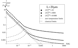
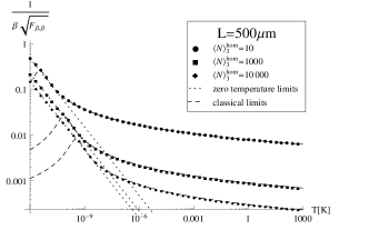
Figure 1: Log-log-plot of the optimal relative error $1/(\beta\sqrt{(F_{d}^{\rm hom})_{\beta,\beta}})$ for a homogenous gas of ⁶Li atoms in three dimensions as function of temperature: $L=20\mu$m (left) and $L=500\mu$m (right); and $\langle N\rangle_{3}^{\rm hom}=10$ (circles), $\langle N\rangle_{3}^{\rm hom}=1000$ (squares), and $\langle N\rangle_{3}^{\rm hom}=10000$ (diamonds). Dotted (dashed) lines are the corresponding small temperature limits (59) (classical limits (57,58)). For a given temperature, we computed the chemical potential inverting the equation of state (42) with the Netown’s method, then we used this result in (45) and plotted the corresponding values of $1/(\beta\sqrt{(F_{d}^{\rm hom})_{\beta,\beta}})$.

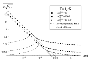
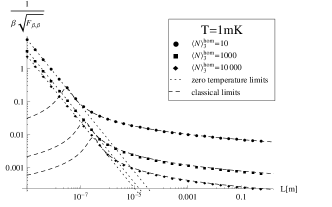
Figure 2: Log-log plot of the optimal relative error $1/(\beta\sqrt{(F_{d}^{\rm hom})_{\beta,\beta}})$ for a homogenous gas of ⁶Li atoms in three dimensions: $T=1$pK (up, left), $T=1$nK (up, right), $T=1\mu$K (down, left), and $T=1$mK (down, right); and $\langle N\rangle_{3}^{\rm hom}=10$ (circles), $\langle N\rangle_{3}^{\rm hom}=1000$ (squares), and $\langle N\rangle_{3}^{\rm hom}=10000$ (diamonds). Dotted (dashed) lines are the corresponding small temperature limits (59) (classical limits (57,58)). For a given $L$, we computed the chemical potential inverting the equation of state (42) with the Netown’s method, then we used this result in (45) and plotted the corresponding values of $1/(\beta\sqrt{(F_{d}^{\rm hom})_{\beta,\beta}})$.

On the other hand, the chemical potential can be measured with almost no error due to the divergence of $(F_{d}^{\rm hom})_{\mu,\mu}/\langle N\rangle_{d}^{\rm hom}$ as $1/T$ for small $T$. If the temperature is exactly zero, all the fermions are frozen in the lowest energies up to the Fermi energy. The smallest change in the chemical potential equals the spacing between the Fermi energy and the next excited state, keeping the temperature fixed. The state consequently changes into an orthogonal state with a different number of particles. This non-smooth change is in contrast with the assumptions upon which the standard quantum Cramér-Rao bound (5) is based, and requires the generalization to non-differentiable models Tsuda2005 . However, this gives an intuition for the divergence of $(F_{d}^{\rm hom})_{\mu,\mu}/\langle N\rangle_{d}^{\rm hom}$ in the regime of small temperatures. In this context, remember that temperature and chemical potential can be jointly measured. We discuss the zero temperature case in more detail in appendix B.

Low temperatures: bosonic gases

In the low-temperature bosonic case (but above the condensation temperature), some of the polylogarithms diverge as ${\rm Li}_{\alpha}(e^{x})=\Gamma(1-\alpha)(-x)^{\alpha-1}+{\cal O}(1)$ for $x\to 0$ and ${\rm Re}(\alpha)<1$. Thus, the prefactors $(F_{d}^{\rm hom})_{\beta,\beta}/\langle N\rangle_{d}^{\rm hom}$ and $(F_{d}^{\rm hom})_{\mu,\beta}/\langle N\rangle_{d}^{\rm hom}$ are finite or zero for all values of the fugacity $e^{\beta\mu}$ in $[0,1]$, while $(F_{d}^{\rm hom})_{\mu,\mu}/\langle N\rangle_{d}^{\rm hom}$ diverges when the fugacity approaches one, namely its value at the critical temperature Huang ; PethickSmith ; PitaevkiiStringari , implying a very precise measurement of the chemical potential. These divergences are ruled by the way the chemical potential approaches zero. In this limit, we derive upper bounds for the Fisher information $(F_{d}^{\rm hom})_{\mu,\mu}$ and the corresponding scaling with $\langle N\rangle_{d}^{\rm hom}$. Since the polylogarithms are continuous functions, the Fisher information $(F_{d}^{\rm hom})_{\mu,\mu}$ assumes all values between (57) in the classical limit and the following bounds (up to inequality (69)) which are saturated at the onset of the BEC.

The value of the chemical potential is constrained by two conditions. The first one is implied by the application of the continuum approximation (41). Indeed, approximating the sum with the integral is valid only for very small momentum spacings, namely small $2\pi\hslash/L_{x,y,z}$, which is the quantity that becomes infinitesimal in the continuum limit. Since $\beta\mu$ is always subtracted from $\beta\varepsilon_{k}$, the validity of the continuum approximation requires that $-\beta\mu$ cannot be smaller than the energy spacing, i.e.

$$-\beta\mu\geqslant\frac{\beta(2\pi\hslash)^{2}}{2mV_{d}^{\frac{2}{d}}}=\frac{\lambda_{T}^{2}\varrho^{\frac{2}{d}}}{(\langle N\rangle_{d}^{\rm hom})^{\frac{2}{d}}},$$ (60)

for homogeneous gases. If at low temperatures (60) is violated one should set $-\beta\mu=0$ in all thermodynamical quantities which do not diverge under this replacement in the continuum approximation. For thermodynamical quantities that would diverge when setting $-\beta\mu=0$ one has to estimate the exact sums over the modes without the continuum approximation, in order to carefully estimate their scaling with the average number of particles.

A second bound is given by the occupation of the ground state:

$$\langle a_{0}^{\dagger}a_{0}\rangle=\frac{1}{e^{-\beta\mu}-1}\leqslant\langle N\rangle_{d}^{\rm hom}\Rightarrow-\beta\mu\geqslant\ln\left(1+\frac{1}{\langle N\rangle_{d}^{\rm hom}}\right)\simeq\frac{1}{\langle N\rangle_{d}^{\rm hom}}.$$ (61)

In three dimensions, the continuum approximation through (60) bounds the Fisher information to

$$(F_{3}^{\rm hom})_{\mu,\mu}\lesssim\frac{\beta^{2}}{\lambda_{T}^{4}\varrho^{\frac{4}{3}}}(\langle N\rangle_{3}^{\rm hom})^{\frac{4}{3}}\simeq\frac{\beta^{2}}{\zeta\left(\frac{3}{2}\right)^{\frac{4}{3}}}(\langle N\rangle_{3}^{\rm hom})^{\frac{4}{3}},$$ (62)

where the last inequality follows from $\lambda_{T}^{3}\rho\simeq\zeta(3/2)$ for small chemical potentials. Smaller chemical potentials, $\ln(1+1/\langle N\rangle_{3}^{\rm hom})\leqslant-\beta\mu\leqslant o(\langle N\rangle_{3}^{\rm hom})^{-2/3}$, are practically zero in the continuum approximation and $(F_{3}^{\rm hom})_{\mu,\mu}$ diverges. From the computation of the discrete sums in this regime, the leading contribution yields

$$(F_{3}^{\rm hom})_{\mu,\mu}\simeq\frac{1}{\mu^{2}}+\frac{\beta^{2}V_{3}^{\frac{4}{3}}}{\pi^{2}\lambda_{T}^{4}}\sum_{(n_{x},n_{y},n_{z})\neq(0,0,0)}\frac{1}{(n_{x}^{2}+n_{y}^{2}+n_{z}^{2})^{2}}\simeq\frac{1}{\mu^{2}}+\frac{16.5\beta^{2}}{\pi^{2}\lambda_{T}^{4}\varrho^{\frac{4}{3}}}(\langle N\rangle_{3}^{\rm hom})^{\frac{4}{3}}\simeq\frac{1}{\mu^{2}}+\frac{16.5\,\beta^{2}}{\pi^{2}\zeta\left(\frac{3}{2}\right)^{\frac{4}{3}}}(\langle N\rangle_{3}^{\rm hom})^{\frac{4}{3}}$$ (63)

for isotropic gases Giorgini1998 ; PitaevkiiStringari , in agreement with the limiting scaling in the continuum approximation, and where the constant $16.5$ was estimated from numerical summation ranging from -256 to 256. The last inequality follows from $\lambda_{T}^{3}\rho\simeq\zeta(3/2)$ for small chemical potentials.

In one and two dimensions, the finiteness of the density $\varrho$ implies the finiteness of the chemical potential $\mu\neq 0$, and thus the finiteness of the prefactors $(F_{1,2}^{\rm hom})_{\mu,\mu}/\langle N\rangle_{1,2}^{\rm hom}$. However, $(F_{1,2}^{\rm hom})_{\mu,\mu}$ exhibits a superlinear scaling with the average number of particles if the volume is fixed rather than the density; similarly, allowing large densities $\varrho$ gives large prefactors $(F_{1,2}^{\rm hom})_{\mu,\mu}/\langle N\rangle_{1,2}^{\rm hom}$. For the two-dimensional case, the explicit dependence of this prefactor is given by (47,48). The conditions (60) and (61) give the same scaling for the chemical potential, which constraints the density, using the estimation of (47) for small chemical potentials: $\lambda_{T}^{2}\varrho\lesssim\ln\langle N\rangle_{2}^{\rm hom}$. The resulting Fisher information is

$$(F_{2}^{\rm hom})_{\mu,\mu}\simeq\beta^{2}\langle N\rangle_{2}^{\rm hom}\frac{e^{\lambda_{T}^{2}\varrho}}{\lambda_{T}^{2}\varrho}\lesssim\beta^{2}\frac{(\langle N\rangle_{2}^{\rm hom})^{2}}{\log\langle N\rangle_{2}^{\rm hom}}.$$ (64)

For extremely high densities in $d=2$ ($\lambda_{T}^{2}\varrho>1$), the condition (60) is more stringent than (61). Both the average number of particles and $(F_{2}^{\rm hom})_{\mu,\mu}$ diverge at zero chemical potentials. For isotropic gases with intermediate chemical potentials between (60) and (61), the dominant contributions of the discrete sums are

$$\langle N\rangle_{2}^{\rm hom} \simeq -\frac{1}{\beta\mu}+\frac{V_{2}}{\pi\lambda_{T}^{2}}\sum_{\begin{subarray}{c}n_{x},n_{y}=0\\ (n_{x},n_{y})\neq(0,0)\end{subarray}}^{{\cal O}\left(\frac{V_{2}}{\pi\lambda_{T}^{2}}\right)}\frac{1}{n_{x}^{2}+n_{y}^{2}}\simeq-\frac{1}{\beta\mu}+\frac{V_{2}}{2\lambda_{T}^{2}}\ln\left(\frac{V_{2}}{\pi\lambda_{T}^{2}}\right),$$ (65)

$$(F_{2}^{\rm hom})_{\mu,\mu} \simeq \frac{1}{\mu^{2}}+\frac{\beta^{2}V_{2}^{2}}{\pi^{2}\lambda_{T}^{4}}\sum_{(n_{x},n_{y})\neq(0,0)}\frac{1}{(n_{x}^{2}+n_{y}^{2})^{2}}\simeq\frac{1}{\mu^{2}}+\frac{6.03\,\beta^{2}}{\pi^{2}\lambda_{T}^{4}\varrho^{2}}(\langle N\rangle_{2}^{\rm hom})^{2}\lesssim\frac{1}{\mu^{2}}+\frac{6.03\,\beta^{2}}{\pi^{2}}\frac{(\langle N\rangle_{2}^{\rm hom})^{2}}{\ln^{2}\langle N\rangle_{2}^{\rm hom}},$$ (66)

where the last inequality holds under the condition $\lambda_{T}^{2}\varrho\gtrsim\ln\langle N\rangle_{2}^{\rm hom}$, opposite to that in the continuum approximation.

In one dimension and at not too large densities $\lambda_{T}\varrho\lesssim\sqrt{\langle N\rangle_{1}^{\rm hom}}$, the continuum approximation gives a more stringent constraint (60) than the physical requirement (61). In the continuum approximation, the limit of large density and $\mu$ close to zero, together with the above bound of the density, give

$$(F_{1}^{\rm hom})_{\mu,\mu}\simeq\frac{\beta^{2}}{2\pi}\lambda_{T}^{2}\varrho^{2}\langle N\rangle_{1}^{\rm hom}\lesssim\frac{\beta^{2}}{2\pi}(\langle N\rangle_{1}^{\rm hom})^{2}.$$ (67)

For higher densities $\lambda_{T}\varrho\gtrsim\sqrt{\langle N\rangle_{1}^{\rm hom}}$, there is an intermediate regime between (60) and (61), where the chemical potential should be set to zero for a consistent application of the continuum approximation. However, since both the average number of particles and $(F_{1}^{\rm hom})_{\mu,\mu}$ diverge at zero chemical potentials, they are estimated by the dominant contributions of the respective discrete sums:

$$\langle N\rangle_{1}^{\rm hom} \simeq -\frac{1}{\beta\mu}+\frac{L_{x}^{2}}{\pi\lambda_{T}^{2}}\sum_{n_{x}=1}^{\infty}\frac{1}{n_{x}^{2}}=-\frac{1}{\beta\mu}+\frac{\pi L_{x}^{2}}{6\lambda_{T}^{2}},$$ (68)

$$(F_{1}^{\rm hom})_{\mu,\mu} \simeq \frac{1}{\mu^{2}}+\frac{\beta^{2}L_{x}^{4}}{\pi^{2}\lambda_{T}^{4}}\sum_{n_{x}=1}^{\infty}\frac{1}{n_{x}^{4}}=\frac{1}{\mu^{2}}+\frac{\pi^{2}\beta^{2}}{90\lambda_{T}^{4}\rho^{4}}(\langle N\rangle_{1}^{\rm hom})^{4}\lesssim\frac{1}{\mu^{2}}+\frac{\pi^{2}\beta^{2}}{90}(\langle N\rangle_{1}^{\rm hom})^{2},$$ (69)

where the last inequality comes from the above high density condition $\lambda_{T}\varrho\gtrsim\sqrt{\langle N\rangle_{1}^{\rm hom}}$.

In Fig. 3, we plot the upper bounds (62,64,67) of the Fisher information $(F_{d}^{\rm hom})_{\mu,\mu}$ within the continuum approximation versus the average number of particles in double logarithmic scale. Since the slope represents the exponent of the dependence of $(F_{d}^{\rm hom})_{\mu,\mu}$ on $\langle N\rangle_{d}^{\rm hom}$, we notice that decreasing the dimensionality, the sensitivity of the chemical potential increases. We compare the curves with the linear scaling (shot-noise) reproduced by the classical limit and the zero temperature case where all the particles occupy the ground state (see section V).

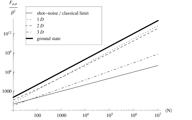
Figure 3: Log-log plot of the upper bounds of the rescaled Fisher information $(F_{d}^{\rm hom})_{\mu,\mu}/\beta^{2}$ for homogenous Bose gas above the condensation temperature against the average number of particles within the continuum approximation in three dimensions (dotdashed line) (62), two dimensions (dashed line) (64), and one dimension (dotted line) (67). The continuous line is the shot-noise reproduced by the classical gas, eq.(57). The thick line is the Fisher information if all particles are in the ground state, namely the zero temperature case, eq.(81).

IV.2 Harmonically trapped ideal gases

For gases confined in a harmonic potential, the thermodynamic limit is defined as $\langle N\rangle_{d}^{\rm harm}\to\infty$ and $\omega_{x,y,z}\to 0$. In order to have a finite density either the quantity $\langle N\rangle_{d}^{\rm harm}\Omega_{d}^{d}$ Mullin1997 ; Mullin2012 or $\langle N\rangle_{d}^{\rm harm}\Omega_{d}^{\frac{d}{2}}$ Beau2010 is fixed. This choice affects the thermodynamics of the gas, such as the phase transition towards a Bose-Einstein condensate Beau2010 ; Mullin2012 . We follow the physical arguments presented in Mullin1997 ; Mullin2012 and define $\tilde{\varrho}\equiv\langle N\rangle_{d}^{\rm harm}\Omega_{d}^{d}$. Since all the quantities (50,51,52,53,54) are proportional to $\Omega_{d}^{-d}$, the entries of the Fisher matrix scale linearly with $\langle N\rangle_{d}^{\rm harm}$. As before, $\mu\in[-\infty,\infty]$ and $\beta\in[0,\infty]$ for fermions, while $\mu\in[-\infty,0)$ and $\beta$ is larger than the critical inverse temperature for bosons in the non-condensed phase. With the above mentioned properties of the polylogarithms, we can study when the prefactors $(F_{d}^{\rm harm})_{\#,\#}/\langle N\rangle_{d}^{\rm harm}$ diverge.

Classical limit

In the classical limit, i.e. $e^{\beta\mu}\ll 1$, the statistical averages and the Fisher matrix are

$$\langle N\rangle_{d}^{\rm harm}\simeq\frac{e^{\beta\mu}}{(\beta\hslash\Omega_{d})^{d}},\qquad\langle H\rangle_{d}^{\rm harm}\simeq\frac{d\,e^{\beta\mu}}{\beta^{d+1}(\hslash\Omega_{d})^{d}},\qquad(F_{d}^{\rm harm})_{\mu,\mu}\simeq\beta^{2}\langle N\rangle_{d}^{\rm harm},$$ (70)

$$(F_{d}^{\rm harm})_{\beta,\beta}\simeq\langle N\rangle_{d}^{\rm hom}\left(\mu^{2}-2d\frac{\mu}{\beta}+\frac{d^{2}+2d}{\beta^{2}}\right),\qquad(F_{d}^{\rm harm})_{\mu,\beta}\simeq\langle N\rangle_{d}^{\rm harm}(\beta\mu-d).$$ (71)

The entries of the Fisher matrix scale linearly with the average number of particles, and equal those of classical gases derived in the appendix A.

As for the homogenous gases, we now investigate physical regimes where the Fisher matrix overcomes the linear scaling with $\langle N\rangle_{d}^{\rm harm}$, which characterizes the classical limit.

Low temperatures: fermionic gases

At small temperatures $\beta\to\infty$, the chemical potential of fermionic gases is close to the Fermi energy $\mu\to E_{F}$, and

$$(F_{d}^{\rm harm})_{\mu,\mu}\simeq\frac{d\beta}{\mu}\langle N\rangle_{d}^{\rm harm},\qquad(F_{d}^{\rm harm})_{\beta,\beta}\simeq\frac{d\pi^{2}}{3\beta^{3}\mu}\langle N\rangle_{d}^{\rm harm},\qquad(F_{d}^{\rm harm})_{\mu,\beta}\simeq\frac{(1-d)d\pi^{2}}{3\beta^{2}\mu^{2}}\langle N\rangle_{d}^{\rm harm}.$$ (72)

As for homogeneous gases, the sensitivity of a temperature measurement is very bad, whereas the chemical potential can be measured with infinitely high sensitivity. The interpretation of the divergence of $(F_{d}^{\rm harm})_{\mu,\mu}$ is the same as for homogeneous fermionic gases: at zero temperature, all the fermions are frozen in the lowest energies up to the Fermi energy, the smallest change of the chemical potential is the spacing between the Fermi energy and the next excited state, and the state suddenly changes into an orthogonal state with a different number of particles. Quantum estimation theory for non-differentiable models Tsuda2005 needs to be applied when the temperature is exactly zero, as discussed in the appendix B.

Low temperatures: bosonic gases

For bosonic gases at low temperature, (but above the condensation temperature), the prefactors $(F_{d}^{\rm harm})_{\beta,\beta}/\langle N\rangle_{d}^{\rm harm}$ and $(F_{d}^{\rm harm})_{\mu,\beta}/\langle N\rangle_{d}^{\rm harm}$ are always finite or zero. However, $(F_{d}^{\rm harm})_{\mu,\mu}/\langle N\rangle_{d}^{\rm harm}$ can diverge when the temperature approaches the critical temperature deGroot1950 ; Mullin1997 ; PethickSmith , corresponding to $\mu\to 0$. This stems from the divergence of the polylogarithms already mentioned for bosonic homogeneous gases. Also for harmonic gases, we derive upper bounds of the scaling of $(F_{d}^{\rm harm})_{\mu,\mu}/\langle N\rangle_{d}^{\rm harm}$ with respect to $\langle N\rangle_{d}^{\rm harm}$, which are saturated at the onset of BEC. The Fisher information $(F_{d}^{\rm harm})_{\mu,\mu}$ varies continuously between its classical limit (70) and the following bounds, due to the continuity of the polylogarithms.

As for the homogeneous gases, the chemical potential is bounded by the energy spacing in the continuum approximation, i.e.

$$-\beta\mu\geqslant\beta\hslash\Omega_{d}=\beta\hslash\left(\frac{\tilde{\varrho}}{\langle N\rangle_{d}^{\rm harm}}\right)^{1/d},$$ (73)

for isotropic confinements. The other bound is given by the occupation of the ground state, i.e.

$$\langle a_{0}^{\dagger}a_{0}\rangle=\frac{1}{e^{-\beta\mu}-1}\leqslant\langle N\rangle_{d}^{\rm harm}\Rightarrow-\beta\mu\geqslant\ln\left(1+\frac{1}{\langle N\rangle_{d}^{\rm harm}}\right)\simeq\frac{1}{\langle N\rangle_{d}^{\rm harm}}.$$ (74)

Therefore, for $\ln(1+1/\langle N\rangle_{2}^{\rm harm})\leqslant-\beta\mu\leqslant o(\langle N\rangle_{2}^{\rm harm})^{-1/d}$, the continuum approximation can break and the discrete sums must be computed, as discussed for the homogeneous gases.

In three dimensions, both $\langle N\rangle_{3}^{\rm harm}$ and $(F_{3}^{\rm harm})_{\mu,\mu}$ remain finite, and for small chemical potentials

$$(F_{3}^{\rm harm})_{\mu,\mu}\simeq\frac{\pi^{2}\beta^{2}}{6\zeta(3)}\langle N\rangle_{3}^{\rm harm}.$$ (75)

In two dimensions, the Fisher information relative to the chemical potential diverges as $(F_{2}^{\rm harm})_{\mu,\mu}/\langle N\rangle_{2}^{\rm harm}\simeq-\frac{6}{\pi^{2}}\beta^{2}\ln(-\beta\mu)$. The condition (73) from the continuum approximation yields

$$(F_{2}^{\rm harm})_{\mu,\mu}\lesssim\frac{3\beta^{2}}{\pi^{2}}\langle N\rangle_{2}^{\rm harm}\ln\langle N\rangle_{2}^{\rm harm}.$$ (76)

Chemical potentials that go to zero faster than (73) for large $\langle N\rangle_{2}^{\rm harm}$ vanish in the continuum approximation, and $(F_{2}^{\rm harm})_{\mu,\mu}$ diverges. The dominant contributions of the discrete sum is

$$(F_{2}^{\rm harm})_{\mu,\mu}\simeq\frac{1}{\mu^{2}}+\frac{1}{\hslash^{2}\Omega_{2}^{2}}\sum_{\begin{subarray}{c}n_{x},n_{y}=0\\ (n_{x},n_{y})\neq(0,0)\end{subarray}}^{{\cal O}\left(\frac{1}{\beta\hslash\Omega_{2}}\right)}\frac{1}{(n_{x}+n_{y})^{2}}=\frac{1}{\mu^{2}}+\frac{\langle N\rangle_{2}^{\rm harm}}{2\hslash^{2}\tilde{\varrho}}\ln\left(\frac{\langle N\rangle_{2}^{\rm harm}}{\beta^{2}\hslash^{2}\tilde{\varrho}}\right).$$ (77)

In one dimension the finiteness of $\tilde{\varrho}$ prevents the chemical potential to vanish. Moreover, the constraints (73) and (74) give the same scaling for the chemical potential. These scaldings together with the estimation of (55) for small chemical potentials imply the following bound for the density: $\beta\hslash\tilde{\varrho}\lesssim\ln\langle N\rangle_{1}^{\rm harm}$. For large $\tilde{\varrho}$ the explicit equations (55,56) imply

$$(F_{1}^{\rm harm})_{\mu,\mu}\simeq\beta\langle N\rangle_{1}^{\rm harm}\frac{e^{\beta\hslash\tilde{\varrho}}}{\hslash\tilde{\varrho}}\lesssim\beta^{2}\frac{(\langle N\rangle_{2}^{\rm harm})^{2}}{\log\langle N\rangle_{1}^{\rm harm}}..$$ (78)

For extremely high densities, there is a remarkable intermediate regime between (60) and (61), where the discrete sums must be evaluated. The dominant contributions of $\langle N\rangle_{1}^{\rm harm}$ and $(F_{1}^{\rm harm})_{\mu,\mu}$ are

$$\langle N\rangle_{1}^{\rm harm} \simeq -\frac{1}{\beta\mu}+\frac{1}{\beta\hslash\omega_{x}}\sum_{n_{x}=1}^{{\cal O}\left(\frac{1}{\beta\hslash\omega_{x}}\right)}\frac{1}{n_{x}}\simeq-\frac{1}{\beta\mu}+\frac{1}{\beta\hslash\omega_{x}}\ln\left(\frac{1}{\beta\hslash\omega_{x}}\right),$$ (79)

$$(F_{1}^{\rm harm})_{\mu,\mu} \simeq \frac{1}{\mu^{2}}+\frac{1}{\hslash^{2}\omega_{x}^{2}}\sum_{n_{x}\geqslant 1}\frac{1}{n_{x}^{2}}=\frac{1}{\mu^{2}}+\frac{\pi^{2}}{6\hslash^{2}\tilde{\varrho}^{2}}\left(\langle N\rangle_{1}^{\rm harm}\right)^{2}\lesssim\frac{1}{\mu^{2}}+\frac{\pi^{2}\beta^{2}}{6}\frac{\left(\langle N\rangle_{1}^{\rm harm}\right)^{2}}{\ln^{2}\langle N\rangle_{1}^{\rm harm}},$$ (80)

where the last inequality holds for densities larger than those in the continuum approximation, $\beta\hslash\tilde{\varrho}\gtrsim\ln\langle N\rangle_{1}^{\rm harm}$.

In Fig. 4, we plot the upper bounds (75,76,78) of the Fisher information $(F_{d}^{\rm harm})_{\mu,\mu}$ versus $\langle N\rangle_{d}^{\rm harm}$ within the continuum approximation in double logarithmic scale. As, for homogeneous gases, we see that the smaller the dimensionality, the better the sensitivity of the chemical potential. The curves are compared with the classical limit that exibits shot-noise, i.e. a linear scaling, and the zero temperature case where all the particles occupy the ground state. Figs. 3 and 4 show that harmonic gases exhibit worse sensitivities than homogeneous gases with the same dimension, in accordance with the scalings in the formulas.

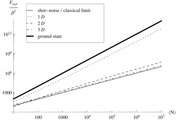
Figure 4: Upper bounds of the rescaled Fisher information $(F_{d}^{\rm harm})_{\mu,\mu}/\beta^{2}$ for harmonically trapped bosons above the condensation temperature against the average number of particles in double logarithmic scale within the continuum approximation in three dimensions (dotdashed line) (75), two dimensions (dashed line) (76), and one dimension (dotted line) (78). The continuous line is the shot-noise reproduced by the classical gas. The thick line is the Fisher information if all particles are in the ground state, i.e. the zero temperature case.

V Fisher matrix in the presence of Bose-Einstein condensation

Bosonic gases experience a phase transition towards Bose-Einstein condensation. This occurs when a macroscopic number of particles occupy a vanishingly small number of states. These states are either the only ground state in the case of normal Bose-Einstein condensation, or a band of states for the so-called generalized Bose-Einstein condensation.

The conventional approach to the Bose-Einstein condensation Huang ; PethickSmith ; PitaevkiiStringari ; Reichl consists in finding the maximum average number of particles within the continuum limit, i.e. substituting the sum over the modes with an integral. If the actual number of particles is larger, the continuum limit breaks, and the sum over the modes has to be replaced by the corresponding integral plus a singular measure. The latter is a delta-like measure that singles out the contribution of a zero measure subset of states. This describes the emergence of the Bose-Einstein condensate above the critical density $\varrho_{c}=\max_{\mu}\varrho$ ($\tilde{\varrho}_{c}=\max_{\mu}\tilde{\varrho}$) or equivalently below the critical temperature $T_{c}$ defined by the relation $\varrho(T_{c})=\varrho_{c}$ ($\tilde{\varrho}(T_{c})=\tilde{\varrho}_{c}$).

Now, we discuss the sensitivity in the estimation of $(\beta,\mu)$ in the presence of different kinds of Bose-Einstein condensations.

V.1 Normal Bose-Einstein condensation

If the density is finite, homogeneous ideal gases with isotropic confinement ($L_{x}=L_{y}=L_{z}$) exhibit a normal Bose-Einstein condensation only in three dimensions, with critical temperature $T_{c}=\frac{2\pi\hslash^{2}}{k_{B}m}\left(\frac{\varrho}{\zeta(3/2)}\right)^{2/3}$ and fraction of condensate $f=1-(T/T_{c})^{3/2}$ Huang ; PethickSmith ; PitaevkiiStringari ; Reichl . Harmonically trapped ideal gases with the same trap frequency in each direction ($\omega_{x}=\omega_{y}=\omega_{z}$) undergo Bose-Einstein condensation in $d=2,3$ dimensions, with critical temperatures $T_{c}=\frac{\hslash}{k_{B}}\left(\frac{\tilde{\varrho}}{\zeta(d)}\right)^{1/d}$ and fraction of condensate $f=1-(T/T_{c})^{d}$ Mullin1997 . We now focus on the condensed phase of these gases.

Below the critical temperature $T<T_{c}$ the chemical potential is very small at finite size, $-\beta\mu={\cal O}(1/\langle N\rangle)$, and the contribution of the ground state must be singled out in the sums. The average number of particles below the critical temperature is $\langle N\rangle=\langle N_{0}\rangle+\langle N_{\rm ex}\rangle$, where $N_{0}=a_{0}^{\dagger}a_{0}$ is the number of particles in the ground state, $\langle N_{0}\rangle=(e^{-\beta\mu}-1)^{-1}=f\langle N\rangle$, $N_{\rm ex}=N-N_{0}$ is the number of particles in the excited states, and $\langle N_{\rm ex}\rangle$ is given by (42) or (50) within the continuum approximation. The estimation of $\langle N_{0}\rangle$ at small chemical potentials gives the evaluation of the chemical potential itself $-\beta\mu\simeq 1/(f\langle N\rangle)$. Since the modes are independent in the grand canonical state, the variance of the total number of particles is $\Delta^{2}N=\Delta^{2}N_{0}+\Delta^{2}N_{\rm ex}$, where $\Delta^{2}N_{0}$ is the variance of the number of particles condensed in the ground state and $\Delta^{2}N_{\rm ex}$ is the variance of the number of particles in the excited states. The computation at small but finite $\mu$, that is at finite size, gives $\Delta^{2}N_{0}=e^{\beta\mu}(1-e^{\beta\mu})^{-2}=\langle N_{0}\rangle+\langle N_{0}\rangle^{2}$. The scaling of the chemical potential violates the conditions (60,73), thus $\Delta^{2}N_{\rm ex}$ must be evaluated at zero chemical potential and via the computation of the discrete sum if its continuum approximation diverges at $\mu=0$. The leading contribution is the same as (63), (75) or (77) without the term $1/\mu^{2}$ and divided by $\beta^{2}$. On the other hand, applying the theory of spontaneous symmetry breaking, one finds that $\Delta^{2}N_{0}=0$, the mode operators of the ground states being replaced by numbers through the Bogolioubov shift Yukalov2005 .

This apparent ambiguity is sorted out by noticing that the symmetry breaking approach can be applied only in the thermodynamic limit. In this limit, the grand canonical thermal state without symmetry breaking is thermodynamically unstable because the isotermal compressibility (12) diverges. Thus, the gas splits up into two phases, one consisting of all particles in the ground state without particle number fluctuations while the other is the non-condensed phase where statistical averages equal those for the excited states. However, the grand canonical thermal state can be considered at finite size, even if its instability grows with the number of particles as argued after equation (12). Moreover, the Bogoliubov shift is not always a good approximation of exact physical behaviours Gaul2013 .

The computation of the particle number variance straightforwardly gives the Fisher information of the chemical potential via (38). If the symmetry breaking approach is considered, the variance $\Delta^{2}N$ and the Fisher information reduce to that of the non-condensed phase, namely (63), (75) or (77) without the term $1/\mu^{2}$. In particular, the Fisher information scales superlinearly with the number of particles for the three-dimensional homogeneous gas and the two-dimensional harmonically trapped gas. If the grand canonical thermal state without the symmetry breaking is considered, the Fisher information $F_{\mu\mu}$ is increased by the superlinear contribution due to the ground state,

$$\beta^{2}\Delta^{2}N_{0}=\beta^{2}\left(f\langle N\rangle+f^{2}\langle N\rangle^{2}\right).$$ (81)

Equation (81) follows directly from the proportionality relation between the Fisher information and the variance of the total number of particles (38), and from the above considerations on the variance. This quadratic scaling dominates over the contribution of the excited states, and also the three-dimensional harmonically trapped gas exhibits sub-shot-noise.

The contributions of the ground state to the other entries of the Fisher matrix do not scale superlinearly in the condensed phase: the ground state contribution to $F_{\beta,\beta}$ is $\beta^{-2}$, and the contribution to $F_{\mu,\beta}$ is $(\beta\mu)^{-1}=-f\langle N\rangle$. Even if the presence of the BEC does not increase the sensitivity of the temperature estimation beyond the shot-noise, it is worthwhile to compute such sensitivity in the spirit of a recent experiment Leanhardt2013 . In this experiment, a harmonically trapped three-dimensional gas of ²³Na atoms has been prepared below the condensation critical temperature, and the lowest measured temperature was $450\pm 80$pK. Since even in the condensed phase the ground state contribution to $F_{\beta,\beta}$ does not dominate, $F_{\beta,\beta}$ is always represented by the thermal averages (45,53) taken at $\beta\mu=0$. These considerations give the following Fisher information for the homogeneous and harmonic gases in the condensed phase:

$$(F_{d})_{\beta,\beta}^{\rm hom}=\frac{(d^{2}+2d)\zeta\left(\frac{d}{2}+2\right)m^{\frac{d}{2}}V_{d}}{2^{2+\frac{d}{2}}\pi^{\frac{d}{2}}\hslash^{d}\beta^{2+\frac{d}{2}}},\qquad(F_{d})_{\beta,\beta}^{\rm harm}=\frac{(d+d^{2})\zeta(d+1)}{\hslash^{d}\beta^{d+2}\Omega_{d}^{d}}.$$ (82)

First, we observe that the Fisher information given by (82) decreases with decreasing temperature the faster the larger the dimension. Thus, lower dimensions provide better sensitivities for low temperature thermometry. Remember that there is a condensed phase at non-zero temperature only in two and three dimensions for the hamonically trapped gas, and only in three dimensions for the homogeneous gas. Interestingly, equations (82) also provide the leading order of the expansion around zero temperature for bosonic gases where there is no phase transition, i.e. no condensed phase at non-zero temperature. In order to show this, one can invert the equation of state (42,50) to find the function $\mu(\beta)$, plug it into (45,53), and then perform a single limit $\beta\to\infty$ using the properties of polylogarithms Wood1992 . The inversion of the equation of state can be done analytically for the two-dimensional homogeneous gas (47) and the one-dimensional harmonically trapped gas (55), due to the simple analytical form, while for the one-dimensional homogeneous gas it can be done in the limit of small chemical potential with ${\rm Li}_{\alpha}(-e^{x})=-x^{\alpha}/\Gamma(\alpha+1)-\pi^{2}x^{\alpha-2}/(6\Gamma[\alpha-1])+{\cal O}(x^{\alpha-4})$ for $Re(x)\gg 1$ Wood1992 . Intuitively, the fugacity $e^{\beta\mu}$ and the density (42,50) are infinitesimal in the limit $\beta\to\infty$, approaching rather the classical limit than the small temperature limit, unless $\mu\to 0$ such that $\beta\mu\to 0$. This indicates why equations (80) are the leading order of the small temperature limit in the absence of phase transition, even if they were derived taking $\mu\to 0$ before $\beta\to\infty$.

The above $F_{\beta,\beta}$ can be used to derive a lower bound for the relative error of the temperature estimation. Note that, in the limit $T\to 0$, the relative error of the optimal estimation $1/(\beta\sqrt{(F_{d})_{\beta,\beta}})\leqslant\sqrt{\rm var(\beta)}/\beta=\Delta T/T$ diverges as $1/T^{d/4}$ for homogeneous gases and $1/T^{d/2}$ for harmonic gases. However, the optimal relative error is small in actual experiments: for instance, in the case of the experiment Leanhardt2013 , i.e. $\omega_{x}=2\pi(0.65\pm 0.05)$Hz, $\omega_{y}=2\pi(1.2\pm 0.1)$Hz, $\omega_{z}=2\pi(1.81\pm 0.05)$Hz, and $T=450$pK, we get $1/(\beta\sqrt{(F_{3}^{\rm harm})_{\beta\beta}})\simeq 0.011$. Our bound is one order of magnitude smaller than the experimental error $80/450\simeq 0.18$, suggesting that the realized sensitivity can be improved.

V.2 Normal Bose-Einstein condensation under isobaric cooling

A different behaviour of bosonic gases occurs when the temperature is lowered at constant pressure, instead of constant volume, in ideal homogeneous bosonic gases in two dimensions with vanishing boundary conditions Gunther1974 : $\varepsilon_{k}=(k_{x}^{2}+k_{y}^{2})/(2m)$, with $k_{x,y}=\frac{\pi}{L}n_{x,y}$ and $n_{x,y}=1,2,3,\dots\,\,$. Under isobaric cooling, the density diverges, and all the dependences on the volume must be carefully considered. This explains why this kind of Bose-Einstein condensation depends on the boundary conditions, because boundary conditions affect the scaling of the ground state energy with respect to the volume Gunther1974 . In this example, a transition towards a normal Bose-Einstein condensation takes place at temperature $T_{c}=\sqrt{\frac{12\hslash P}{\pi mk_{B}}}$. Equations (42,43,44,45,46) hold above the critical temperature. The volume is sub-extensive when it approaches $T_{c}$ from above or below $T_{c}$ (i.e. the volume scales sublinearly with the number of particles), and the density diverges. A divergent particle density is a known mechanism to overcome no-go theorems Penrose1956 ; Hohenberg1967 ; Krueger1967 ; Chester1968 ; Girardeau1969 ; Chester1969 for Bose-Einstein condensation in low dimensions Sonin1969 ; Rehr1970 ; Mullin1997 ; Mullin2000 . Approaching the critical temperature, the density is $\varrho=\langle N\rangle/V_{2}\simeq-\sqrt{\frac{3mP}{\pi^{3}\hslash^{2}}}\ln(T/T_{c}-1)$, as computed in Gunther1974 . Hence $F_{\mu,\mu}$ scales superlinearly with $\langle N\rangle$ as in equation (64), but not $F_{\beta,\beta}\simeq\frac{\pi^{2}}{3\beta^{2}\lambda_{T}^{2}\varrho}\langle N\rangle$ and $F_{\mu,\beta}\simeq\langle N\rangle\left(1-\frac{1}{\lambda_{T}^{2}\varrho}\right)$.

Below the critical temperature we need to single out the contribution of the ground state in the sums. This contribution to $F_{\mu,\mu}$ is $\beta\Delta^{2}N_{0}=\beta^{2}(\langle N_{0}\rangle+\langle N_{0}\rangle^{2})$ which would imply a quadratic scaling in the Fisher information. However, applying the theory of spontaneous symmetry breaking, the variance $\Delta^{2}N_{0}$ vanishes because the number of particles in the condensate is approximated with a number. Moreover, the contribution of the excited states comes from the continuum approximation of the non-condensed gas. However, the integral in $F_{\mu,\mu}$ diverges , and we need to compute the discrete sum, whose leading order comes from the behaviour of small momenta. This contribution is the same as (66) without the term $1/\mu^{2}$, and scales as $V_{2}^{2}$. Since below the critical temperature the non-extensive scaling of the volume is $V_{2}={\cal O}(\sqrt{\langle N\rangle})$, the previous Fisher information scales linearly in the average number of particles. However, at the edge of the transition $\langle N\rangle={\cal O}(V_{2}\ln V_{2})$, thus the Fisher information scales more than linearly with the average number of particles $F_{\mu,\mu}/\langle N\rangle={\cal O}(V_{2}/\ln V_{2})$.

As pointed out before, $F_{\beta,\beta}$ and $F_{\mu,\beta}$ scale at most linearly with the average number of particles both in the ground state contribution and in the excited state contribution within the continuum approximation.

V.3 Generalized Bose-Einstein condensation and dimensional confinement

A different kind of condensation, called generalized Bose-Einstein condensation, occurs when a band of states of zero measure is macroscopically occupied, rather than only the ground state. Examples are ideal gases confined in anisotropic homogeneous or harmonic potentials. If the confinement is much stronger in some directions, the contributions of the excited energy levels in the less confined directions dominate below the critical temperature. In other words, the condensation occurs only in the ground state of the more confined directions, and an effective lower dimensional gas is realized. A hierarchy of condensations is possible: from a three-dimensional gas to a two or one dimensional gas, and from a two dimensional gas to a one dimensional gas. Generalized Bose-Einstein condensation has been studied both at finite size and in the thermodynamic limit focusing on the mathematical structure and general properties of quantum gases Girardeau1960 ; Girardeau1965 ; Casimir1968 ; Krueger1968 ; Rehr1970 ; vandenBerg1982 ; vandenBerg1983 ; vandenBerg1986 ; Ketterle1996 ; vanDruten1997 ; Mullin1997 ; Zobay2004 ; Beau2010 ; Mullin2012 , in connection with liquid helium in thin films Osborne1949 ; Mills1964 ; Khorana1964 ; Goble1966 , magnetic flux of superconducting rings Sonin1969 , and gravito-optical traps Wallis1996 . Experimental realizations with trapped atoms have been reported in Gorlitz2001 ; Greiner2001 ; Esteve2006 ; vanAmerongen2008 ; vanAmerongen2008-2 ; Bouchoule2011 ; Armijo2011 . We shall discuss estimation sensitivity of $(\beta,\mu)$ in the presence of condensation into lower dimensional gases. The scheme is the following: first prepare a three-dimensional gas in the grand canonical thermal state with a fixed density, then lower the temperature until the onset of the generalized condensation. Afterwards, the gas can be employed for the estimation with sensitivity given by the Fisher matrix.

For the sake of concreteness, we consider an ideal homogeneous gas confined in a slab, namely a box of dimension $L_{x}\times L_{y}\times L_{z}$ with $L_{x,y}\gg L_{z}$, where condensation in a two-dimensional gas occurs Osborne1949 ; Goble1966 ; Krueger1968 ; Sonin1969 ; vanDruten1997 ; Beau2010 . This system is also analytically convenient because the average number of particles and the Fisher information relative to the chemical potential of the two-dimensional homogeneous gas have simple expressions (47,48). Note also the formal similarity with the ideal gas confined in a cigar-like harmonic potential Ketterle1996 ; Mullin1997 ; vanDruten1997 ; Beau2010 ; Mullin2012 , because both the two-dimensional ideal gas in a box potential and the one-dimensional ideal gas in a harmonic potential have a constant density of states.

The critical density and the critical temperature of the three-dimensional gas are respectively $\varrho_{c}^{\rm 3D}=\zeta(3/2)/\lambda_{T}^{3}=\varrho\,(T/T_{c}^{\rm 3D})^{3/2}$ and $T_{c}^{\rm 3D}=\frac{2\pi\hslash^{2}}{k_{B}m}\left(\frac{\varrho}{\zeta(3/2)}\right)^{2/3}$. If $\varrho>\varrho_{c}^{\rm 3D}$ and $T<T_{c}^{\rm 3D}$, a number of particles $f\langle N\rangle$, with $f=1-(T/T_{c}^{\rm 3D})^{3/2}$, condenses in a small part of the modes. Since $L_{x,y}\gg L_{z}$, the occupancies $(e^{\beta(\varepsilon_{k}-\mu)}-1)^{-1}$ of the energy levels with $n_{z}\neq 0$ are negligible compared to the others, below the critical temperature. The remaining modes form a two-dimensional gas consisting of energy levels with $n_{z}=0$, and the number of particles confined there is given by (42), namely $\langle N\rangle_{2}^{\rm hom}\simeq-\frac{L_{x}L_{y}}{\lambda_{T}^{2}}\ln(\beta|\mu|)$ for small $\beta|\mu|$. If these states constitute the condensate then $\langle N\rangle_{2}^{\rm hom}=f\varrho\,L_{x}L_{y}L_{z}$ and $\beta|\mu|\simeq e^{-f\varrho\lambda_{T}^{2}L_{z}}$. Moreover, in order for the occupancies of the modes with $n_{z}=0$ to contribute with a singular measure in the continuum limit, the chemical potential should satisfy $\beta\varepsilon_{(k_{x},k_{y},0)}\leqslant|\beta\mu|\simeq e^{-f\varrho\lambda_{T}^{2}L_{z}}\ll\beta\varepsilon_{(0,0,k_{z}\neq 0)}$. This implies that $L_{x}=L_{y}\geqslant\gamma e^{\alpha L_{z}}$ for some constant $\alpha$ independent of $L_{z}$ and some function $\gamma(L_{z})$ that does not suppress the exponential scaling with $L_{z}$.

In order to find the behaviour of $\gamma$ in the thermodynamic limit, we now compare the chemical potential with the first excited energy in the transversal directions, $x$ and $y$, i.e. $\varepsilon_{(1,0,0)}=\pi\lambda_{T}^{2}/(\beta L_{x}^{2})$. The number of particles in the two-dimensional condensate $\langle N\rangle_{2}^{\rm hom}$ grows when $\beta|\mu|$ decreases, and is estimated in the deep two-dimensional condensate phase by its value at $\beta|\mu|\simeq\beta\varepsilon_{(1,0,0)}$. The latter is the condition for the possible onset of a second condensation in the ground state alone where the energy of all the excited states is neglible compared to the energy scale $\beta|\mu|$. If $L_{x}=L_{y}\ll\gamma e^{\alpha L_{z}}$, the gas directly condenses in the ground state without the intermediate two-dimensional condensate, and indeed $\beta|\mu|\simeq\beta\varepsilon_{(1,0,0)}$ implies $\langle N\rangle_{2}^{\rm hom}/V_{3}\ll 2\alpha/\lambda_{T}^{2}-\ln(\pi\lambda_{T}^{2}/\gamma^{2})/(\lambda_{T}^{2}L_{z})$. This evaluation for the two-dimensional occupation is compatible with the absence of a two-dimensional condensate, i.e. $\langle N\rangle_{2}^{\rm hom}\ll 1$, provided $(\ln\gamma/\lambda_{T})/L_{z}\to 0$ when $L_{z}\to\infty$. In the opposite limit $L_{x}=L_{y}\gg\gamma e^{\alpha L_{z}}$, $\langle N\rangle_{2}^{\rm hom}/V_{3}\gg 2\alpha/\lambda_{T}^{2}-\ln(\pi\lambda_{T}^{2}/\gamma^{2})/(\lambda_{T}^{2}L_{z})$ implies that the number of particles in the two-dimensional condensate grows indefinitely with decreasing $\beta|\mu|$. In the absence of a saturation, there is no further condensation towards the ground state. Such saturation occurs if $L_{x}=L_{y}=\gamma e^{\alpha L_{z}}$: $\langle N\rangle_{2}^{\rm hom}/V_{3}\simeq 2\alpha/\lambda_{T}^{2}-\ln(\pi\lambda_{T}^{2}/\gamma^{2})/(\lambda_{T}^{2}L_{z})\to 2\alpha/\lambda_{T}^{2}$ in the thermodynamic limit. Thus, there is a second critical density $\varrho_{c}^{\rm 2D}=\varrho_{c}^{\rm 3D}+2\alpha/\lambda_{T}^{2}$: when the density approaches $\varrho_{c}^{\rm 2D}$ the chemical potential scales as $\beta|\mu|\simeq e^{-2\alpha L_{z}}$, whereas if $\varrho>\varrho_{c}^{\rm 2D}$ a second condensation with a macroscopic fraction of particles in the ground state occurs and the chemical potential scales as the inverse of the three-dimensional volume.

One can also derive the temperature $T_{c}^{\rm 2D}$ below which the occupation of the ground state dominates over the other modes of the two-dimensional gas, at finite size. This temperature is found by imposing that the density equals the second critical density: $\rho(T_{c}^{\rm 2D})=\rho_{c}^{\rm 2D}$, equivalent to $\zeta(3/2)\lambda_{T_{c}^{\rm 2D}}^{-3}+2\alpha\lambda_{T_{c}^{\rm 2D}}^{-2}=\rho$, where $\lambda_{T_{c}^{\rm 2D}}$ is the thermal wavelength evaluated at the second critical temperature Beau2010 . As mentioned above, a two-dimensional gas does not condense in the ground state if the usual thermodynamic limit is considered, with the density fixed and finite. The reason of such a condensation here is that the number of particles in the two-dimensional gas is proportional to the total number of particles of the original three-dimensional gas, thus to the three-dimensional volume, and the two-dimensional density $\langle N\rangle_{2}^{\rm hom}/(L_{x}L_{y})=g\varrho L_{z}$ diverges in the thermodynamic limit. We will see that this is also the reason for a superlinear scaling of the Fisher information as soon as a condensation in a two-dimensional gas occurs.

We focus on the temperature regime $T_{c}^{\rm 2D}\leqslant T\leqslant T_{c}^{\rm 3D}$, where the number of particles in the two-dimensional gas is $\langle N\rangle_{2}^{\rm hom}=\langle N\rangle-\rho_{c}^{\rm 3D}V_{3}=f\langle N\rangle$. The macroscopic occupation of a vanishingly small number of modes, namely the two-dimensional gas, below the first critical temperature cannot be described by the continuum approximation of the eigenenergies. Thus, the contributions of the condensate must be singled out from the integral (41) in the thermodynamic averages. For instance, the average number of particles is Beau2010 ; Mullin2012

$$\langle N\rangle=\langle N\rangle_{2}^{\rm hom}+\langle N\rangle_{3}^{\rm hom}=\frac{V_{3}}{\lambda_{T}^{2}L_{z}}\ln(1-e^{\beta\mu})+\frac{V_{3}}{\lambda_{T}^{3}}\,{\rm Li}_{\frac{3}{2}}(e^{\beta\mu})=f\varrho V_{3}+\frac{1}{\lambda_{T}^{3}}\,{\rm Li}_{\frac{3}{2}}(e^{\beta\mu})$$ (83)

Similarly, the entries of the Fisher matrix are the sum of three- and two-dimensional contributions: at the leading orders for large $L_{z}$,

$$F_{\mu,\mu} = (F_{2}^{\rm hom})_{\mu,\mu}+(F_{3}^{\rm hom})_{\mu,\mu}=\frac{\beta^{2}L_{x}L_{y}}{\lambda_{T}^{2}}\left(e^{f\varrho\lambda_{T}^{2}L_{z}}-1\right)+\frac{\beta^{2}V_{3}}{\lambda_{T}^{3}}{\rm Li}_{\frac{1}{2}}(e^{\beta\mu}),$$ (84)

$$F_{\beta,\beta} = (F_{2}^{\rm hom})_{\beta,\beta}+(F_{3}^{\rm hom})_{\beta,\beta}$$ (85)

$$\simeq \frac{L_{x}L_{y}}{3\beta^{2}\lambda_{T}^{2}}\left(\pi^{2}-3e^{-f\varrho\lambda_{T}^{2}L_{z}}\right)+\frac{V_{3}}{\beta^{2}\lambda_{T}^{3}}\left(\beta^{2}\mu^{2}{\rm Li}_{\frac{1}{2}}(e^{\beta\mu})-3\beta\mu{\rm Li}_{\frac{3}{2}}(e^{\beta\mu})+\frac{15}{4}{\rm Li}_{\frac{5}{2}}(e^{\beta\mu})\right),$$

$$F_{\mu,\beta} = (F_{2}^{\rm hom})_{\mu,\beta}+(F_{3}^{\rm hom})_{\mu,\beta}\simeq\frac{L_{x}L_{y}}{\lambda_{T}^{2}}\left(-1+\frac{e^{-f\varrho\lambda_{T}^{2}L_{z}}}{2}\right)-f\varrho\,V_{3}+\frac{V_{3}}{\lambda_{T}^{3}}\left(\beta\mu{\rm Li}_{\frac{1}{2}}(e^{\beta\mu})-\frac{3}{2}{\rm Li}_{\frac{3}{2}}(e^{\beta\mu})\right).$$ (86)

The entries $F_{\beta,\beta}$ and $F_{\mu,\beta}$ are linear in the volume, thus in the average number of particles $\langle N\rangle$. On the other hand

$$\frac{F_{\mu,\mu}}{\langle N\rangle}=\frac{\beta^{2}}{\varrho\lambda_{T}^{2}L_{z}}\left(e^{f\varrho\lambda_{T}^{2}L_{z}}-1\right)+\frac{\beta^{2}}{\varrho\lambda_{T}^{3}}{\rm Li}_{\frac{1}{2}}(e^{\beta\mu}).$$ (87)

The two contributions, coming respectively from the two-dimensional condensate and the three-dimensional bulk, diverge as $L_{z}\to\infty$. To see the divergence of the contribution from the three-dimensional cloud, we recall that the chemical potential between the two critical temperatures satisfies $\beta|\mu|\simeq e^{-f\varrho\lambda_{T}^{2}L_{z}}$. This value is larger than the minimum energy spacing, that is $\beta(2\pi\hslash)^{2}/(2m\gamma^{2}e^{2\alpha L_{z}})$, thus the continuum approximation still holds in analogy to the discussion of the bound (41). Therefore, for small chemical potentials the approximation ${\rm Li}_{1/2}(e^{\beta\mu})=\sqrt{\pi/(\beta|\mu|)}+{\cal O}(1)$ implies that the last term of $F_{\mu,\mu}/\langle N\rangle$ behaves as $\frac{\sqrt{\pi}\beta^{2}}{\varrho\lambda_{T}^{3}}\,e^{f\varrho\lambda_{T}^{2}L_{z}/2}$.

In particular, if $L_{x}=L_{y}=\gamma e^{\alpha L_{z}}$, then $\gamma^{2}L_{z}e^{2\alpha L_{z}}=V_{3}=\langle N\rangle/\varrho$ and $2\alpha L_{z}\simeq\ln(V_{3}/\ell^{3})$, for large $L_{z}/\ell$ where $\ell$ is a characteristic length, e.g. $\ell=\lambda_{T}$ or $\ell=1/\alpha$. Thus,

$$\frac{F_{\mu,\mu}}{\langle N\rangle}=\frac{2\alpha\beta^{2}}{\varrho\lambda_{T}^{2}\ln\frac{\langle N\rangle}{\varrho\,\ell^{3}}}\left(\left(\frac{\langle N\rangle}{\varrho\,\ell^{3}}\right)^{\frac{f\varrho\lambda_{T}^{2}}{2\alpha}}-1\right)+\frac{\sqrt{\pi}\beta^{2}}{\varrho\lambda_{T}^{3}}\left(\frac{\langle N\rangle}{\varrho\,\ell^{3}}\right)^{\frac{f\varrho\lambda_{T}^{2}}{4\alpha}}.$$ (88)

Fig. 5 is the log-log plot of the Fisher information in equation (88) against the average number of particles at different temperatures between the two critical temperatures. The slopes show inceasing superlinear scalings comprised between the classical limit exhibiting a linear scaling and the zero temperature case, i.e. all particles in the ground state. Below the second critical temperature, a macroscopic number of particles $\langle N_{0}\rangle$ occupy the ground state. The contribution of this second BEC must be singled out from statistical averages. As discussed in section V.1, its contribution to the Fisher information $F_{\mu,\mu}$ is $\beta^{2}(\langle N_{0}\rangle+\langle N_{0}\rangle^{2})$. Thus, a quadratic scaling emerges with an increasing weight when temperature decreases.

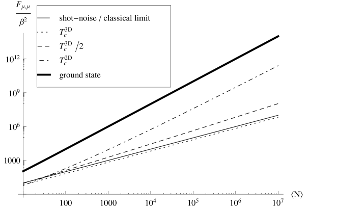
Figure 5: Double logarithmic plot of the rescaled Fisher information $F_{\mu,\mu}/\beta^{2}$ of an ideal bose gas versus the average number of particles of a gas of ⁸⁷Rb atoms in a slab with exponential anisotropy $L_{x,y}\sim\gamma e^{\alpha L_{z}}$. The curves refer to different temperatures: classical limit (continuous line, linear in $\langle N\rangle$), first critical temperature $T_{c}^{\rm 3D}=100$nK (dotted line), $T_{c}^{\rm 3D}/2$ (dashed line), second critical temperature $T_{c}^{\rm 2D}=20$nK (dotdashed line), zero temperature (thick continuous line, quadratic in $\langle N\rangle$ (see eq.(81))). The two critical temperatures are uniquely determined by $\rho=13\cdot 10^{12}$cm^-3 and $\alpha=10\mu$m^-1. Furthermore, $\ell=\lambda_{T}$.

We emphasize that the one-dimensional ideal gas trapped in a harmonic potential has mathematically similar properties as the two dimensional ideal gas in an infinite square potential. In particular, a three-dimensional harmonically trapped gas with frequencies $\omega_{x,y,z}$ in the three directions can be confined to the $x$ direction if $\omega_{x}\ll\omega_{y,z}$, as studied in Ketterle1996 ; Mullin1997 ; vanDruten1997 ; Beau2010 ; Mullin2012 . The equations for the average number of particles and the Fisher matrix in the condensed phase are the sum of three- and one-dimensional contributions, similarly to the above discussed case of homogeneous gas. For instance,

$$\frac{F_{\mu,\mu}}{\langle N\rangle}=\frac{\beta\omega_{y}\omega_{z}}{\tilde{\varrho}\hslash}\left(e^{\frac{\hslash\beta\tilde{\varrho}}{\omega_{y}\omega_{z}}}-1\right)+\frac{{\rm Li}_{2}(e^{\beta\mu})}{\tilde{\varrho}\beta\hslash^{3}},$$ (89)

which diverges in the thermodynamic limit. Notice that now the contribution from the three-dimensional harmonically trapped gas ${\rm Li}_{2}(e^{\beta\mu})$ is always bounded, unlike the analogous contribution in the case of the square potential.

VI Fisher matrix with interacting Bose gases

In this section we discuss how the interactions modify the aforementioned superlinear scaling of the Fisher information $F_{\mu,\mu}$. It is already known that small interactions can wipe out the superlinear scaling of $F_{\mu,\mu}$, for the three-dimensional homogeneous gas below the critical temperature Huang ; Yukalov2005 . We now consider three models of interactions which have different effects on the Fisher information. The first model describes harmonic interactions which preserve the superlinear scalings discussed above. Then, we discuss mean field interactions for which a complete analytic solution can be computed, resulting in the suppression of the superlinear scaling of the Fisher information unless the interaction strength is very small. Finally, we consider contact interactions which do not allow a general analytic computation but can be treated perturbatively for small interactions. This regime, that is experimentally accessible Armijo2011 , is characterized by only small deviations from sub-shot-noise. In the latter two models, there is a tradeoff between the smallness of the interaction and the strength of the sub-shot-noise: the stronger the gain over the shot-noise, the weaker the interaction must be in order to preserve sub-shot-noise.

VI.1 Harmonic interactions

A simple model for interacting systems is given by harmonic interactions Madelung08 . Consider for the moment the interacting hamiltonian at the level of first quantization, e.g.

$$H_{\rm 1st}=\sum_{j}\left(\frac{{\bf p}_{j}^{2}}{2m}+\frac{m\omega^{2}{\bf r}_{j}^{2}}{2}\right)+\sum_{j,l}\gamma({\bf r}_{j}-{\bf r}_{l})^{2},$$ (90)

where ${\bf p}_{j}$ and ${\bf r}_{j}$ are respectively the momentum and the position of the $j$-th particle. The hamiltonian is a quadratic form in the variables $\{{\bf p}_{j},{\bf r}_{j}\}_{j}$. Therefore, via a rotation in the phase-space $(\tilde{\bf p}_{1},\tilde{\bf r}_{1},\tilde{\bf p}_{2},\tilde{\bf r}_{2},\dots)=R({\bf p}_{1},{\bf r}_{1},{\bf p}_{2},{\bf r}_{2},\dots)$ where $R$ is an orthogonal matrix, the hamiltonian can be recast into a non-interacting-like hamiltonian $\tilde{H}_{\rm 1st}=\sum_{j}\left(\frac{\tilde{\bf p}_{j}^{2}}{2\tilde{m}}+\frac{\tilde{m}\tilde{\omega}^{2}\tilde{\bf r}_{j}^{2}}{2}\right)$. Moving to the second quantization, we have a problem formally similar to that of an ideal gas in a harmonic potential, discussed in the previous sections. The interactions in this model are hidden in the phase-space rotation which maps single particle operators and modes into collective operators and modes. Thus, the above considerations on harmonically trapped gases apply with the substitution $\omega_{x,y,z}\to\tilde{\omega}_{x,y,z}$.

VI.2 Mean field interaction

Here, we focus on the Bose gas with mean field interaction, also known as imperfect Bose gas. The hamiltonian is $H=H_{0}+\lambda N^{2}/(2V_{d})$, where $H_{0}$ is the hamiltonian of the ideal gas as in (30), $N$ is the total number operator (1), $V_{d}$ is the volume, and $\lambda$ is the interaction strength. $\lambda$ is positive for repulsive interactions, that always take place at small distances. This statistical model has been solved in vandenBerg1984 , for a general class of non-interacting hamiltonians independently of the dimensionality. The grand canonical thermodynamic potential, i.e. the pressure, is:

$$p_{\lambda}=\frac{1}{V_{d}\beta}\ln Z_{G}^{(\lambda)}=\frac{(\mu-\alpha(\mu))^{2}}{2\lambda}+p_{0}(\alpha(\mu)),$$ (91)

where $Z_{G}^{(\lambda)}$ is the grand canonical partition function of the mean field model, $p_{0}=\lim_{\lambda\to 0}p_{\lambda}$ is the pressure of the non interacting gas, $\alpha(\mu)$ is zero if $\mu\geqslant\lambda\rho_{c}$ and is the unique solution of $\alpha+\lambda\,\partial_{\alpha}p_{0}(\alpha)=\mu$ if $\mu<\lambda\rho_{c}$, and $\rho_{c}$ if the critical density which coincides with that of the non-interacting hamiltonian. From the thermodynamic potential we can compute all the statistical averages, for instance

$$\langle N\rangle_{\lambda} = \frac{1}{\beta}\frac{\partial}{\partial\mu}\ln Z_{G}^{(\lambda)}=\frac{V_{d}}{\lambda}(\mu-\alpha(\mu)),$$ (92)

$$\Delta^{2}_{\lambda}N = \frac{1}{\beta^{2}}\frac{\partial^{2}}{\partial\mu^{2}}\ln Z_{G}^{(\lambda)}=\frac{V_{d}}{\beta}\frac{\partial^{2}_{\alpha}p_{0}(\alpha)}{1+\lambda\,\partial^{2}_{\alpha}p_{0}(\alpha)}=\frac{V_{d}\Delta^{2}_{0}N}{V_{d}+\lambda\beta\Delta^{2}_{0}N},$$ (93)

$$F_{\mu,\mu}^{(\lambda)} = \beta^{2}\Delta^{2}_{\lambda}N=\frac{V_{d}\beta F_{\mu,\mu}^{(0)}}{V_{d}\beta+\lambda F_{\mu,\mu}^{(0)}}.$$ (94)

From these computations, we learn that the imperfect Bose gas has the same critical density as the ideal gas with the same non-interacting hamiltonian. In particular, there is the same hierarchy of condensation mentioned in the previous section: a three-dimensional gas condenses into a two-dimensional gas which may condense in the unique ground state. However, the thermodynamic properties differ from those of the ideal gas. For instance, the Fisher information $F_{\mu,\mu}^{(\lambda)}$ always scales at most linearly with the volume, for finite interaction strengths. Indeed, even if $F_{\mu,\mu}^{(0)}$ scales superlinearly with the average number of particles, then $F_{\mu,\mu}^{(\lambda)}\simeq V_{d}\beta/\lambda$, i.e. is simply extensive due to the proportionality of the volume $V_{d}$ to the total particle number, unless $\lambda\ll V_{d}\beta/F_{\mu,\mu}^{(0)}$. This happens both in the three-dimensional bulk and in the lower dimensional condensate.

If the ideal system exhibits a superlinear scaling of the Fisher information, the bound $\lambda\ll V_{d}\beta/F_{\mu,\mu}^{(0)}$ goes to zero for infinite size. In this limit, the superlinear scaling disappears for any coupling constant, but at finite size there are values of $\lambda$ which do not destroy the sub-shot-noise.

VI.3 Contact interaction

From a theoretical perspective, the study of Bose-Einstein condensation in statistical mechanics becomes a highly non-trivial problem in the presence of interactions, see Zagrebnov2001 for a review. In particular, the condensation is driven not only by the decreasing of temperature but also by the presence of interactions. This implies the coexistence of different condensates and a complex structure of the states occupied in the condensed phases, without a clear extension of the generalized Bose-Einstein condensation in lower dimensional gases. On the other hand, a kinematic approach was investigated to prove dimensional confinement Olshanii1998 , later implemented in mesoscopic systems Gorlitz2001 ; Greiner2001 ; Esteve2006 ; vanAmerongen2008 ; vanAmerongen2008-2 ; Bouchoule2011 ; Armijo2011 . This approach consists in proving that the scattering amplitudes of a three-dimensional bosonic gas with contact interactions and a strong harmonic confinement in two transverse dimensions correspond to those of an effective one-dimensional gas, if the incident wave is frozen in the transverse ground state and its longitudinal kinetic energy is smaller than the energy spacing of the transverse potential. The effective one dimensional gas is described by the Yang-Yang model which was formally solve in Yang1968 .

The hamiltonian of the model is

$$H=\sum_{k}\frac{k^{2}}{2m}a_{k}^{\dagger}a_{k}+\frac{c}{2L_{x}}\sum_{k_{1},k_{2},q}a_{k_{1}-q}^{\dagger}a_{k_{2}+q}^{\dagger}a_{k_{2}}a_{k_{1}},$$ (95)

and its statistical properties are relevant in a number of experiments that realize this system Gorlitz2001 ; Esteve2006 ; vanAmerongen2008 ; vanAmerongen2008-2 ; Bouchoule2011 ; Armijo2011 . The peculiarity of this statistical model is that the excitations at infinite interaction strength behave as non-interacting fermions, while of course they are single-particle bosonic modes for vanishing interactions. It is desirable for applications to know the Fisher matrix in the presence of contact interaction.

The formal computation of statistical averages involves the solution of two coupled nonlinear integral equations, which can be solved only numerically. Nevertheless, some analytical results were derived, such as the second order coherence function $g^{(2)}$ in different regimes perturbatively for weak and strong interactions Deuar2009 . Thus, we focus on the Fisher information of the chemical potential $F_{\mu,\mu}$ which shows sub-shot-noise in the limit of zero interaction and for high densities or fixed volumes (67). Given the second order coherence function, we can compute the variance of the total number of particles, and then the Fisher information $F_{\mu,\mu}$ (6). The relation between the second order coherence function and the total number variance is reported in (115) and proved in appendix C.

Different regimes are parametrized by the two dimensionless quantities, $\gamma=\frac{2\pi\beta c}{\lambda_{T}^{2}\varrho}$ and $\tau=\frac{4\pi}{\lambda_{T}^{2}\varrho^{2}}$. The $g^{(2)}$ function for strong interactions, $\gamma\gg 1$, exhibits the typical fermionic anti-bunching behaviour, namely $0\leqslant g^{(2)}\leqslant 1$ Deuar2009 . This property causes a reduction in the variance $\Delta^{2}N$, and thus of $F_{\mu,\mu}$, with respect to the shot-noise, as is clear from equation (115). On the other hand, bunching $g^{(2)}>1$, typical of non-interacting bosons, is responsible of a superlinear scaling of $\Delta^{2}N$ and $F_{\mu,\mu}$ with $\langle N\rangle$. The quantum degenerate gas with small interactions, $\sqrt{\gamma}\ll\tau\ll 1$, is close to the ideal bosonic gas. Therefore, the $g^{(2)}$ function was derived in Deuar2009 within perturbation theory in the coupling constant $c$:

$$g^{(2)}(r)=1+\left(1-\frac{4\gamma}{\tau^{2}}\left(1+\varrho\tau r\right)\right)e^{-\varrho\tau r}.$$ (96)

Plugging this formula into equation (115), we get the Fisher information

$$F_{\mu,\mu} = \beta^{2}\langle N\rangle+\frac{\beta^{2}\lambda_{T}^{2}\varrho^{2}}{2\pi}\langle N\rangle-\frac{\beta^{2}\lambda_{T}^{4}\varrho^{4}}{8\pi^{2}}\left(1-e^{-\frac{4\pi}{\lambda_{T}^{2}\varrho^{2}}\langle N\rangle}\right)$$ (97)

$$+c\left(\frac{3\beta^{3}\lambda_{T}^{6}\varrho^{7}}{16\pi^{3}}\left(1-e^{-\frac{4\pi}{\lambda_{T}^{2}\varrho^{2}}\langle N\rangle}\right)-\frac{\beta^{3}\lambda_{T}^{4}\varrho^{5}}{4\pi^{2}}\langle N\rangle\left(2+e^{-\frac{4\pi}{\lambda_{T}^{2}\varrho^{2}}\langle N\rangle}\right)\right).$$

The condition $\sqrt{\gamma}\ll\tau$ is equivalent to $c\ll\frac{8\pi}{\beta\lambda_{T}^{2}\varrho^{3}}$, and $\tau\ll 1$ reads $\lambda_{T}^{2}\varrho^{2}\gg 4\pi$. Notice that the Fisher information $F_{\mu,\mu}$ scales linearly with $\langle N\rangle$, if the density $\varrho=\langle N\rangle/L_{x}$ is fixed. Instead, if the size $L_{x}$ is fixed, superlinear scaling emerges.

Let us consider the first line of (97), that is the Fisher information of the ideal gas. The second contribution in the first line of (97), $\frac{\beta^{2}\lambda_{T}^{2}}{2\pi L_{x}^{2}}\langle N\rangle^{3}$, is exactly the Fisher information already found for the one-dimensional ideal gas with small chemical potentials, hence large number of particles. It could seem that the third contribution in the first line of (97) scales quartically with $\langle N\rangle$, for fixed $L_{x}$, and thus dominates. This is impossible, since this contribution is negative and the Fisher information is non-negative by definition. However, condition (61) and equation (42) for small chemical potentials imply $\lambda_{T}^{2}\varrho^{2}\lesssim\pi\langle N\rangle$. Thus, for very large numbers of particles $\langle N\rangle\gg\frac{\lambda_{T}^{2}\varrho^{2}}{4\pi}\gg 1$, and the absolute value of the third term is therefore much smaller than the second one.

Now we consider the second line of (97), namely the corrections to the ideal gas due to small interactions. These contributions are linear in $\langle N\rangle$ if the density is fixed, but they scale superlinearly if the size $L_{x}$ is fixed. The last term in (97) dominates for $\langle N\rangle\gg\frac{\lambda_{T}^{2}\varrho^{2}}{4\pi}\gg 1$, and the leading order of the correction due to the interactions is negative, and its absolute value is much smaller than the leading order without interactions:

$$-c\,\frac{\beta^{3}\lambda_{T}^{4}}{2\pi^{2}L_{x}^{5}}\langle N\rangle^{6}\ll-\frac{4\beta^{2}\lambda_{T}^{2}}{\pi L_{x}^{2}}\langle N\rangle^{3}.$$ (98)

The inequality is a consequence of the condition $\sqrt{\gamma}\ll\tau\Leftrightarrow c\ll\frac{8\pi}{\beta\lambda_{T}^{2}\varrho^{3}}$. Since the corrections to the Fisher information are negative, interactions counteract the sub-shot-noise. However, the corrections are much smaller that the Fisher information without interactions. Hence, the sub-shot-noise of one-dimensional homogeneous ideal gases is robust against the detrimental effect of small contact interactions $c\ll\frac{8\pi}{\beta\lambda_{T}^{2}\varrho^{3}}$. Sub-shot-noise can be observed at fixed volume or high density. This condition reduces the range of admissible coupling constants. Moreover, the condition $\tau\ll 1$ implies $\lambda_{T}^{2}\varrho^{2}\ll 4\pi$, thus $c\ll 2/\beta$. It is also interesting that the bound $\frac{8\pi}{\beta\lambda_{T}^{2}\varrho^{3}}$ increases with the temperature. Although (97) is the first perturbative order, a superlinear scaling of the particle fluctuations, thus of the Fisher information, was experimentally observed at fixed volume even beyond the condition $\sqrt{\gamma}\ll\tau$ Armijo2011 .

In Fig. 6, we plot the perturbative formula (97) at different interaction strengths in double logarithmic scale. The sudden drop in the curves is a signature of the failure of the perturbative expansion, where additional terms are required. First, we notice that decreasing the interaction, the superlinear regime is observed for larger average number of particles. Moreover, we considered ⁸⁷Rb atoms confined in a fixed size $L_{x}=4.5\,\mu$m at temperature $T=510\,$nK. These are the parameters of a recent experiment where superlinear particle number fluctuations were observed even beyond the perturbative regime close to the non-interacting case Armijo2011 . Our results are in agreement with the experimental data, considering that the Fisher information of the chemical potential is proportional to the particle number fluctuations, and taking into account the experimental sensitivity of the camera and the depletion of particles in the transversal excited states as explained in the article Armijo2011 . Furthermore, this experiment implies that it is possible to check the quantum sensitivity for the estimation of the chemical potential in one-dimensional interacting gases.

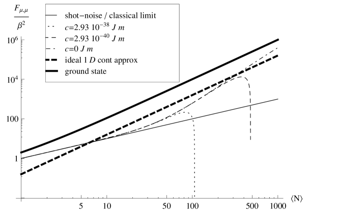
Figure 6: Log-log plot of the rescaled Fisher information $F_{\mu,\mu}/\beta^{2}$ in the perturbative regime (97) against the average number of particles. The results are for a gas of ⁸⁷Rb atoms confined in $L_{x}=4.5\,\mu$m at $T=510\,$nK and interaction strength $c=2.93\cdot 10^{-40}$ J m (dotted line), $c=2.93\cdot 10^{-38}$ J m (dashed line), and $c=0$ (dotdashed line). The continuous line is the shot-noise resulting from the classical limit, the thick dashed line is the best scaling achievable within the continuum approximation (67), and the thick line is the Fisher information if all particles are in the ground state, i.e. the zero temperature case.

VII Conclusions

In summary, we have given a detailed investigation of the sensitivity with which temperature and chemical potential of quantum gases can be measured. This was done by calculating the Quantum Fisher information matrix first for ideal fermionic and bosonic gases, and then examining three different models of interacting gases. In agreement with previously known results we have shown that the best sensitivity of temperature measurements of ideal quantum gases shows SQL-like scaling with the number of particles, both for fermionic and bosonic gases, and irrespective of whether or not the latter are close to the condensation transition. As function of temperature, the relative error diverges as $1/\sqrt{T}$ for homogeneous and harmonically trapped fermionic gases, as $1/T^{d/4}$ for homogenesous BECs, and as $1/T^{d/2}$ for harmonically trapped BECs. This demonstrates that in addition of the impossibility of reaching absolute zero temperature according to the third law of thermodynamics, it also becomes increasingly difficult to measure how close to absolute zero temperature one is. The relative uncertainty increases more rapidly for bosons than for fermions at small temperatures and dimensions larger than one, reflecting the bunching behavior of the bosons.

The sensitivity for measurements of the chemical potential, which has immediate applications to the ultimate precision of voltage measurements in electrical conductors, has a richer behaviour. While for fermions the SQL, corresponding to a linear scaling of the quantum Fisher information with the particle number $N$, cannot be surpassed, bosonic gases allow in principle enhanced sensitivity beyond the SQL. We have shown this in different scenarios: standard isochoric BEC; isobaric BEC; and generalized BEC in 2D or 1D samples, where a hierarchy of condensation transitions can arise, with condensation first taking place in a subspace of Hilbert space. The superlinear scaling of the Fisher information relative to the chemical potential originates in the macroscopic occupation and the consequent bunching induced fluctuations in the occupation of the eigenstates of the BEC. Furthermore, the superlinear scaling never beats the fluctuations at $T=0$ that scale quadratically with $N$. These results are not modified in a simple model of harmonic interactions. However, in a model of mean-field interactions the super-linear scaling of the quantum Fisher information is destroyed, unless the interactions are very small. Small contact interactions, treated in perturbation theory, lead to small corrections of the super-linear scaling of the quantum Fisher information in one-dimensional quantum degenerate gas, and indicate that the chemical potential of bosons can indeed be measured with sub-SQL sensitivity.

We stress that the two parameters can be jointly estimated. This is an unusual feature of quantum multivariate estimation, and stems from the fact that our problem can be recast as a classical statistical problem in the representation of eigenstates of the energy and the particle number. The optimal joint estimation consists in measuring $\mu N-H$ and $N$, while the optimal single parameter estimation of temperature (chemical potential) can be achieved via the measurement of $\mu N-H$ ($N$). The number of particles is measured with absorption imaging in a number of experiments Muller2010 ; Sanner2010 ; Armijo2011 , while the temperature estimation and the corresponding optimal measurement of $\mu N-H$ is hard to implement. The experimental observation of particle number fluctuations in the light of the present analysis opens the possibility for future realizations of quantum sensors based on the measurement of the chemical potential. Furthermore, superlinear sensitivities can be achieved by different physical systems, such as dipolar BEC where superpoissonian particle number fluctuations have been numerically computed Bisset2013 .

Acknowledgement U.M. acknowledges funding by Centre national de la recherche scientifique, by Deutsche Forschungsgemeinschaft, and by Evaluierter Fonds der Albert Ludwigs-Universitaet Freiburg.

Appendix A Classical gases and quantum gases of distinguishable particles

In this appendix, we derive the Fisher matrix for classical ideal gases and quantum ideal gases of distinguishable particles. The latter case is equivalent to the former: once the grand canonical thermal state of the quantum gas is written in its eigenbasis in first quantization, the computation of the partition function and all the statistical averages is same as the for the classical gas. Indeed, distinguishable particles fulfill the Maxwell-Boltzmann counting and they both suffer from the Gibbs’ paradox. Thus, we shall discuss only classical gases.

The hamiltonian of $N$ particles of an ideal gas is the sum of single particles hamiltonians $H=\sum_{j=1}^{N}H_{j}$, where $H_{j}$ is the hamiltonian of the $j$-th particle. Consider a gas of identical classical particles, $H_{j}=H_{1}$ for all $j$. The grand canonical partition function is

$$Z_{G}=\sum_{N=0}^{\infty}\frac{(e^{\beta\mu}Z_{c})^{N}}{N!}=e^{e^{\beta\mu}Z_{C}},$$ (99)

where $Z_{C}=\sum_{H_{1}}e^{-\beta H_{1}}$ is the canonical partition function of the single particle problem, and the factor $N!$ is the cure to the Gibbs’ paradox Huang ; Reichl . This factor arises naturally in the classical limit of quantum gases, i.e. for high temperature and low density equivalent to $e^{\beta\mu}\ll 1$ Huang . Define the single particle mean energy $\langle H_{1}\rangle=-\partial\ln Z_{C}/\partial\beta$ and its variance $\Delta^{2}H_{1}=\partial^{2}\ln Z_{C}/\partial\beta^{2}$. From the partition function, we compute the average number of particles, the average total energy, and the Fisher matrix:

$$\langle N\rangle=e^{\beta\mu}Z_{C},\qquad\langle H\rangle=\langle N\rangle(\langle H_{1}\rangle-\mu),$$ (100)

$$F_{\mu,\mu}=\beta^{2}\Delta^{2}N=\beta^{2}\langle N\rangle,$$ (101)

$$F_{\beta,\beta}=\Delta^{2}(\mu N-H)=\langle N\rangle((\mu-\langle H_{1}\rangle)^{2}+\Delta^{2}H_{1}),$$ (102)

$$F_{\mu,\beta}=F_{\beta,\mu}=\beta\,{\rm Cov}(N,\mu N-H)=\beta\langle N\rangle(\mu-\langle H_{1}\rangle).$$ (103)

Notice that the entries of the Fisher matrix scale lineraly with the average number of particles, in accordance with the shot-noise.

For the homogeneous gas in $d$ dimensions, the single particle hamiltonian is $H_{1}=\frac{p^{2}}{2m}$ which gives $Z_{C}=V_{d}(2\pi m/\beta)^{d/2}$, $\langle H_{1}\rangle=d/(2\beta)$, and $\Delta^{2}H_{1}=d/(2\beta^{2})$. For the $d$-dimensional gas in a harmonic potential, the single particle hamiltonian is $H_{1}=\frac{p^{2}}{2m}+\frac{1}{2}m\omega^{2}x^{2}$ which gives $Z_{C}=(2\pi m/\beta)^{d/2}$, $\langle H_{1}\rangle=d/\beta$, and $\Delta^{2}H_{1}=d/\beta^{2}$. For quantum gases of distinguishable particles all with the same single particle hamiltonian, one has to consider the sum over the eigenvalues of $H_{1}$ in $Z_{C}$. The computations provide prefactors depending on $\hslash$, which do not affect statistical averages with respect to classical gases.

Appendix B Estimation problem for ideal fermionic gases at zero temperatures

One of the assumptions for the validity of the quantum Cramér-Rao bound is the differentiability of the density matrix, as is evident from the formula of the Fisher matrix (4). If this assumption is not met, the quantum Cramér-Rao bound is generalized by the quantum Hammerseley-Chapman-Robbins-Kshirsagar bound Tsuda2005 . The Fermi-Dirac distribution involved in the grand canonical thermal state (32) is the step function at zero temperature. This means that all the particles occupy the eigenstates of the hamiltonian with energy smaller than the chemical potential. At zero temperature the chemical potential is changed only if an additional particle occupies the first empty eigenstate. Thus, the smallest change of the chemical potential is the energy difference between the two eigenstates, and the new thermal state is orthogonal to the original one. This implies a non-continuous change of the density matrix, and the state is not differentiable with respect to the chemical potential.

We now consider the estimation of the chemical potential, following the theory for non-differentiable models. Since the temperature should be set to zero, in order to have a non-differentiable thermal state, we focus on the single parameter estimation of the chemical potential. The starting point is to define a finite change of the chemical potential, say $\delta$, and the finite ratio

$$\Delta_{\delta}\rho_{\beta,\mu}=\frac{\rho_{\beta,\mu+\delta}-\rho_{\beta,\mu}}{\delta}.$$ (104)

This ratio plays the role played by the derivative in the Fisher matrix. The symmetric logarithmic derivatives are generalized by the operators $L_{\mu,\delta}$, defined by

$$\Delta_{\delta}\rho_{\beta,\mu}=\frac{1}{2}\{\rho_{\beta,\mu},L_{\mu,\delta}\},$$ (105)

and the Fisher information is replaced by the following quantity

$$J_{\mu,\delta}={\rm tr}(\rho_{\beta,\mu}L_{\mu,\delta}^{2})={\rm tr}(\Delta_{\delta}\rho_{\beta,\mu}L_{\mu,\delta}).$$ (106)

Finally, the quantum Hammerseley-Chapman-Robbins-Kshirsagar bound reads

$${\rm var}(\mu)\geqslant\frac{1}{J_{\mu,\delta}},$$ (107)

that corresponds to the quantum Cramér-Rao bound if $\delta\to 0$ and the density matrix is differentiable. The inequality (107) is sharp, and the measurement that provides an estimation of $\mu$ with the minimum uncertainty is a projective measurement on the eigenbasis of $L_{\mu,\delta}$, i.e. a measurement of the energy and the number of particles.

If the Fermi energy is degenerate, the thermal state at zero temperature $\rho_{\beta=\infty,\mu}$ is an equally weighted mixture of several pure states. Denote $g$ its degeneracy. The explicit computation in the eigenbasis of the thermal state gives the following result

$$J_{\mu,\delta}=\frac{g}{\delta^{2}}.$$ (108)

At T=0, if the chemical potential is directly tuned, the smallest change $\delta$ is the energy spacing. The finite parallelepiped-shaped quantization volumes of homogeneous two- and three-dimensional gases discussed here break the rotational symmetry. This has some consequences on the energy spacing. Consider isotropic volumes $L_{x}=L_{y}=L_{z}=L$ and Fermi momentum almost parallel to one quantization axis or plane, i.e. only few excitations in at least one direction, say $n_{x}\sim{\cal O}(1)$. The distance between the corresponding Fermi energy and the nearest level is ${\cal O}\left(\frac{\hslash^{2}}{mV_{d}^{2/d}}\right)$. On the other hand, if the Fermi energy is characterized by momenta with large wave numbers $n_{x}\sim n_{y}\sim n_{z}\sim{\cal O}(\eta L)$ with some constant $\eta$, the spacing to the next enery level is ${\cal O}\left(\frac{\hslash^{2}\eta}{mV_{d}^{1/d}}\right)$. These two different scalings give two different regimes for the sensitivity: $J_{\mu,\delta}\sim{\cal O}\left(\frac{gm^{2}}{\hslash^{4}\varrho^{\frac{4}{d}}}(\langle N\rangle_{d}^{\rm hom})^{\frac{4}{d}}\right)$ and $J_{\mu,\delta}\sim{\cal O}\left(\frac{gm^{2}}{\hslash^{4}\eta^{2}\varrho^{\frac{2}{d}}}(\langle N\rangle_{d}^{\rm hom})^{\frac{2}{d}}\right)$ respectively, where only the first scaling is superlinear when the density is finite and $d>1$. Notice that the Fermi energies which provide the faster scaling of the sensitivity are rare, because only a few wave number satisfy $n_{x}\sim{\cal O}(1)$.

This difference originates in the above mentioned break of the rotational symmetry which splits some energy levels. Indeed, if the quantization volume is finite and spherical, the eigenenergies $\frac{p^{2}}{2m}$ depend only on one quantum number, i.e. the quantized modulus of the momentum $p$ which scales with the finite radius of the box as $p\sim{\cal O}(\hslash/R)={\cal O}(\hslash/V_{d}^{1/d})$ Messiah . Thus, given the modulus of the Fermi momentum $k_{F}$, the energy spacing and the sensitivity are

$$\delta\sim{\cal O}\left(\frac{\hslash k_{F}}{mV_{d}^{\frac{1}{d}}}\right),\qquad J_{\mu,\delta}\sim{\cal O}\left(\frac{gm^{2}}{\hslash^{2}k_{F}^{2}\varrho^{\frac{2}{d}}}(\langle N\rangle_{d}^{\rm hom})^{\frac{2}{d}}\right).$$ (109)

If the density $\varrho=\langle N\rangle_{d}^{\rm hom}/V_{d}$ is fixed, the scaling of $J_{\mu,\delta}$ with the average number of particles is sub-linear in three dimensions, linear in two dimensions and superlinear in one dimension. Note that the square and the spherical quantization volume coincide in one dimension, and thus only the result (109) applies. For harmonically trapped isotropic gases,

$$\delta=\hslash\Omega_{d},\qquad J_{\mu,\delta}=\frac{g}{\hslash^{2}\tilde{\varrho}^{\frac{2}{d}}}(\langle N\rangle_{d}^{\rm harm})^{\frac{2}{d}}.$$ (110)

If the density $\tilde{\varrho}=\langle N\rangle_{d}^{\rm harm}\Omega_{d}^{d}$ is fixed, $J_{\mu,\delta}$ has the same scaling as in (109).

The absence of superlinear scaling in more than one dimension can be understood with the presence of high degeneracy in the energy eigenspaces which becomes continuous in the limit of infinite volume. Indeed, the energy depends only on the modulus of $\bf p$ in (41) or of $\bf x$ in (49). Therefore, when the chemical potential is changed, the new particles or holes are spread on the entire eigenspace. Since the optimal measurement is a projective measurement onto the Fock states, i.e. eigenstates of the total number of particles, the continuous degeneracy of the Fermi surface in two and three dimensions makes the measurement more difficult than in one dimension with a two-fold degeneracy. To further investigate the role of the continuous degeneracy, consider anisotropies that break this degeneracy. We now focus on gases in an anisotropic harmonic potential, for the simplicity of the linear energy spacing, with frequencies $\omega_{x}=\omega/\alpha_{x}$, $\omega_{y}=\omega/\alpha_{y}$, $\omega_{z}=\omega/\alpha_{z}$, finite $\omega$, and $\alpha_{x}>\alpha_{y}\geqslant\alpha_{z}$. The typical energy spacing and the corresponding sensitivity for large anisoptropies $\alpha_{x}\gg\alpha_{y,z}$ are given by

$$\delta=\hslash\frac{\omega_{x}}{\alpha_{x}},\qquad J_{\mu,\delta}=\frac{g\alpha_{x}^{2}}{\hslash^{2}\omega^{2}}.$$ (111)

If $\alpha_{x}=\alpha_{y}^{n}=\alpha_{z}^{n}$, the density is $\tilde{\varrho}=\langle N\rangle_{3}^{\rm harm}\omega^{3}\alpha_{x}^{-1-2/n}$, and the inverse sensitivity

$$J_{\mu,\delta}=\frac{g\,\omega^{4\frac{n-1}{n+2}}}{\hslash^{2}\tilde{\varrho}^{\frac{2n}{n+2}}}(\langle N\rangle_{3}^{\rm harm})^{\frac{2n}{n+2}}$$ (112)

scales superlinearly with the average number of particles for $n>2$. The fastest possible scaling is quadratic and achieved for $n\to\infty$.

A different situation occurs if one tunes a continuous parameter, e.g. the voltage or any potential, that leads to jumps of the chemical potential. In this case, $\delta$ can be arbitrary small, for instance one can increase the voltage by an arbitrary small amount $\delta$, until the overall change of the total chemical potential equals the energy spacing. At this point, the density matrix suddenly changes into an orthogonal state, so that the change in the chemical potential is detected with high accuracy.

Appendix C Second order coherence function and the variance of the particle number

In this appendix, we prove the relation between the second order coherence function and the variance of the particle number for homogeneous one-dimensional gases. Consider the field operator $\Psi^{\dagger}(x)$, namely the creation operator of a particles localized in position $x$. Field operators of bosonic particles satisfy commutation relations $[\Psi(x),\Psi^{\dagger}(x^{\prime})]=\delta(x-x^{\prime})$, while fermionic field operators satisfy anti-commutation relations $\{\Psi(x),\Psi^{\dagger}(x^{\prime})\}=\delta(x-x^{\prime})$. The second order coherence function is defined as

$$g^{(2)}(x,x^{\prime})=\frac{\langle\Psi^{\dagger}(x)\Psi^{\dagger}(x^{\prime})\Psi(x^{\prime})\Psi(x)\rangle}{\langle\Psi^{\dagger}(x)\Psi(x)\rangle\langle\Psi^{\dagger}(x^{\prime})\Psi(x^{\prime})\rangle}.$$ (113)

The total number operator is $N=\int dx\Psi^{\dagger}(x)\Psi(x)$. Therefore, with the help of the (anti)commutation relations, the variance of the total number of particles can be written as

$$\Delta^{2}N = \int dxdx^{\prime}\left(\langle\Psi^{\dagger}(x)\Psi(x)\Psi^{\dagger}(x^{\prime})\Psi(x^{\prime})\rangle-\langle\Psi^{\dagger}(x)\Psi(x)\rangle\langle\Psi^{\dagger}(x^{\prime})\Psi(x^{\prime})\rangle\right)$$ (114)

$$= \langle N\rangle+\int dxdx^{\prime}\langle\Psi^{\dagger}(x)\Psi(x)\rangle\langle\Psi^{\dagger}(x^{\prime})\Psi(x^{\prime})\rangle\left(g^{(2)}(x,x^{\prime})-1\right).$$

The result is the same for bosons and fermions because two exchanges of field operators are required. The hamiltonian of homogeneous gases commutes with the total momentum, and statistical averages depend only on relative distances. Thus, $g^{(2)}(x,x^{\prime})=g^{(2)}(|x-x^{\prime}|)$ and $\langle\Psi^{\dagger}(x)\Psi(x)\rangle=\int dx^{\prime}\langle\Psi^{\dagger}(x^{\prime})\Psi(x^{\prime})\rangle/L_{x}=\varrho$. Exploiting these properties and the change of variables $(x,x^{\prime})\to(r=x-x^{\prime},R=(x+x^{\prime})/2)$ in the previous integral, we get

$$\Delta^{2}N=\langle N\rangle+2\varrho^{2}\int_{0}^{L_{x}}dr(L_{x}-r)\left(g^{(2)}(r)-1\right).$$ (115)

Notice that this equation differs form that presented in Yukalov2005 , which gives the leading contribution for large $L_{x}$.

References

- (1) Robert P. Benedict, Fundamentals of Temperature, Pressure and Flow Measurements, John Wiley & Sons, Inc.; 3rd edition (July 1984)
- (2) J. F. Schooley, NBS/NIST Gas Thermometry From 0 to 660 degree Celsius, J. Res. Natl. Inst. Stand. Technol. 95, 255 (1990)
- (3) L. Spietz, K. W. Lehnert, I. Siddiqi, and R. J. Schoelkopf, Science 300, 1929 (2003)
- Levkivskyi and Sukhorukov (2012) I. P. Levkivskyi and E. V. Sukhorukov Phys. Rev. Lett. 109, 246806 (2012)
- (5) O. Madelung, Introduction to Solid-State Theory, Springer Series in Solid-State Sciences, Springer Berlin Heidelberg (October 10, 2008)
- (6) I. M. Savukov, S. J. Seltzer, M. V. Romalis, K. L. Sauer, Phys. Rev. Lett. 95, 063004 (2005)
- (7) K. Fang et al., Phys. Rev. Lett. 110, 130802 (2013)
- (8) M. Loretz, T. Rosskopf, C. L. Degen, Phys. Rev. Lett. 110, 017602 (2013)
- (9) C. D. Aiello, M. Hirose, P. Cappellaro, Nat. Commun. 4, 1416 (2013)
- (10) S. K. Steinke, S. Singh, P. Meystre, K. C. Schwab, M. Vengalattore, Quantum back-action in spinor condensate magnetometry, arXiv:1211.2870
- (11) Y. Eto et al., Spin-Echo-Based Magnetometry with Spinor Bose-Einstein Condensates, arXiv:1306.1011
- (12) A. Waxman et al., Diamond Magnetometry of Superconducting Thin Films, arXiv:1308.2689
- (13) G. Puentes, G. Waldherr, P. Neumann, J. Wrachtrup, Frequency Multiplexed Magnetometry via Compressive Sensing, arXiv:1308.4349
- Cramér (1946) H. Cramér, Mathematical Methods of Statistics (Princeton University Press, Princeton, NJ, 1946)
- Braunstein and Caves (1994) S. L. Braunstein and C. M. Caves, Phys. Rev. Lett. 72, 3439 (1994)
- Stace (2010) T. M. Stace eprint arXiv:1006.1447v1 (2010)
- Ruostekoski et al. (2009) J. Ruostekoski, C. J. Foot, and A. B. Deb, Phys. Rev. Lett. 103, 170404 (2009)
- Sabin et al. (2013) C. Sabín, A. White, L. Hackermuller, and I. Fuentes, eprint arXiv:1303.6208.
- Caves (1981) C. M. Caves, Phys. Rev. D 23, 1693 (1981)
- Giovannetti et al. (2004) V. Giovannetti, S. Lloyd, and L. Maccone, 306, 1330 (2004)
- Giovannetti et al. (2006) V. Giovannetti, S. Lloyd, and L. Maccone, Phys. Rev. Lett. 96, 010401 (2006)
- Giovannetti et al. (2011) V. Giovannetti, S. Lloyd, and L. Maccone, Nat Photon 5, 222 (2011)
- Boto et al. (2000) A. N. Boto, P. Kok, D. S. Abrams, S. L. Braunstein, C. P. Williams, and J. P. Dowling, Phys. Rev. Lett. 85, 2733 (2000)
- (24) M. J. Holland, K. Burnett, Phys. Rev. Lett. 71, 1355 (1993)
- (25) F. Benatti, R. Floreanini, U. Marzolino, Ann. Phys. 325, 924 (2010)
- (26) F. Benatti, R. Floreanini, U. Marzolino, J. Phys. B 44, 091001 (2011)
- (27) G. Argentieri, F. Benatti, R. Floreanini, U. Marzolino, Int. J. Quant. Inf. 9, 1745 (2011)
- (28) F. Benatti, D. Braun, Phys. Rev. A 87, 012340 (2013)
- Brunelli et al. (2011) M. Brunelli, S. Olivares, and M. G. A. Paris, Phys. Rev. A 84, 032105 (2011)
- Slodi\vcka et al. (2012) L. Slodička, G. Hétet, N. Röck, S. Gerber, P. Schindler, M. Kumph, M. Hennrich, and R. Blatt, Phys. Rev. A 85, 043401 (2012)
- Huelga et al. (1997) S. F. Huelga, C. Macchiavello, T. Pellizzari, A. K. Ekert, M. B. Plenio, and J. I. Cirac, Phys. Rev. Lett. 79, 3865 (1997)
- (32) J. Kołodyński and R. Demkowicz-Dobrzánski, Phys. Rev. A 82, 053804 (2010)
- (33) B. M. Escher, R. L. de Matos Filho, L. Davidovich, Nat. Phys. 7, 406 (2011)
- (34) S. Alipour, M. Mehboudi, A. T. Rezakhani, Dissipative quantum metrology in manybody system of identical particles, arXiv:1302.1115 (2013)
- (35) F. Benatti, S. Alipour, A. T. Rezakhani, Quantum Metrology in Open Systems: A Dissipative Quantum Cramer-Rao Bound, arXiv:1308.5359 (2013)
- (36) C. Gross, and T. Zibold, and E. Nicklas, and J. Esteve, and M. K. Oberthaler, Nature 464, 1165 (2010).
- (37) M. F. Riedel, P. Böhi, Y. Li, T. W. Hänsch, A. Sinatra, and P. Treutlein, Nature 464, 1170 (2010).
- Wolfgramm et al. (2012) F. Wolfgramm, C. Vitelli, F. A. Beduini, N. Godbout, and M. W. Mitchell, Nature Photonics 7, 28 (2013)
- Luis (2004) A. Luis, Phys. Lett. A 329, 8 (2004)
- Luis (2007) A. Luis, Phys. Rev. A 76, 035801 (2007)
- Napolitano et al. (2011) M. Napolitano, M. Koschorreck, B. Dubost, N. Behbood, R. J. Sewell, and M. W. Mitchell, Nature 471, 486 (2011)
- Braun and Martin (2011) D. Braun and J. Martin, Nat Commun 2, 223 (2011)
- (43) D. Braun and J. Martin, eprint arXiv:0902.1213v2.
- (44) P. Zanardi and N. Paunković, Phys. Rev. E 74, 031123 (2006)
- (45) C. W. Helstrom, Quantum Detection and Estimation Theory, Academic Press, New York (1976)
- (46) A. S. Holevo, Probabilistic and Statistical Aspect of Quantum Theory, North-Holland, Amsterdam (1982)
- (47) P. Zanardi, Phys. Rev. Lett. 87, 077901 (2001)
- (48) H. Narnhofer, Phys. Lett. A 310, 423 (2004)
- (49) H. Barnum, E. Knill, G. Ortiz, R. Somma, L. Viola, Phys. Rev. Lett. 92, 107902 (2004)
- (50) H. Barnum, G. Ortiz, R. Somma, L. Viola, Int. J. Theor. Phys. 44, 2127 (2005)
- (51) F. Benatti, R. Floreanini, U. Marzolino, Ann. Phys. 327, 1304 (2012)
- (52) F. Benatti, R. Floreanini, U. Marzolino, Phys. Rev. A 85, 042329 (2012)
- (53) V. I. Yukalov, Phys. Rev. E 72, 066119 (2005)
- (54) T. A. Kaplan, J. Stat. Phys. 122, 1237 (2006)
- (55) C. J. Pethick, H. Smith. Bose-Einstein Condensation in Dilute Gases, Cambridge University Press (2002)
- (56) L. Pitaevskii, S. Stringari. Bose-Einstein Condensation, Oxford University Press (2003)
- (57) K. Huang. Statistical mechanics 2nd ed, John Wiley & Sons, Inc. (1987)
- (58) D. C. Wood. The computation of polylogarithm Technical Report 15-92, University of Kent, Computing Laboratory, University of Kent, Canterbury, UK, June 1992.
- (59) Y. Tsuda, K. Matsumoto, J. Phys. A 38, 1593 (2005)
- (60) L. E. Reichl. A Modern Course in Statistical Physics 2nd ed, John Wiley & Sons, Inc. (1998)
- (61) S. Giorgini, L. P. Pitaevskii, S. Stringari, Phys. Rev. Lett. 80, 5040 (1998)
- (62) S. R. de Groot, G. J. Hooymann, C. A. ten Seldam, Proc. R. Soc. Lond. A 203, 266 (1950)
- (63) C. Gaul, J. Schiefele, arXiv:1305.4120 (2013)
- (64) D. M. Weld, P. Medley, H. Miyake, D. Hucul, D. E. Pritchard, W. Ketterle, Phys. Rev. Lett. 103, 245301 (2009)
- (65) T. Müller, B. Zimmermann, J. Meineke, J.-P. Brantut, T. Esslinger, H. Moritz, Phys. Rev. Lett. 105, 040401 (2010)
- (66) C. Sanner, E. J. Su, A. Keshet, R. Gommers, Y. Shin, W. Huang, W. Ketterle, Phys. Rev. Lett. 105, 040402 (2010)
- (67) Q. Zhou, T.-L. Ho, Phys. Rev. Lett. 106, 225301 (2011)
- (68) A. E. Leanhardt, T. A. Pasquini, M. Saba, A. Schirotzek, Y. Shin, D. Kielpinski, D. E. Pritchard, W. Ketterle, Science 301, 1513 (2013)
- (69) L. Gunther, Y. Imry, D. J. Bergman, J. Stat. Phys. 10, 299 (1974)
- (70) O. Penrose, L. Onsager, Phys. Rev. 104, 576 (1956)
- (71) P. C. Hohenberg, Phys. Rev. 158, 383 (1967)
- (72) D. A. Krueger, Phys. Rev. Lett. 19, 563 (1967)
- (73) C. V. Chester, in Lectures in Theoretical Physics ed. K. T. Mahanthappa, Gordon and Breach, Science Publishers, Inc., New York (1968), Vol. 11B, p. 253
- (74) M. Girardeau, J. Math. Phys. 10, 993 (1969)
- (75) G. V. Chester, M. F. Fisher, N. D. Mermin, Phys. Rev. 185, 760 (1969)
- (76) E. A. Sonin, Sov. Phys. JETP 29, 520 (1969)
- (77) J. J. Rehr, N. D. Mermin, Phys. Rev. B 1, 3160 (1970)
- (78) W. J. Mullin, J. Low Temp. Phys. 106, 615 (1997)
- (79) W. J. Mullin, M. Holzmann, F. Laloë, J. Low Temp. Phys. 121, 263 (2000)
- (80) M. Girardeau, J. Math. Phys. 1, 516 (1960)
- (81) M. Girardeau, J. Math. Phys. 6, 1083 (1965)
- (82) H. B. G. Casimir, in Fundamental problems in statistical mechanics II, edited by E. G. D. Cohen (1968), pp. 188
- (83) D. A. Krueger, Phys. Rev. 172, 211 (1968)
- (84) M. van den Berg, J. T. Lewis, Physics A 110, 550 (1982)
- (85) M. van den Berg, J. Stat. Phys. 31, 623 (1983)
- (86) M. van den Berg, J. T. Lewis, J. V. Pulé, Helv. Phys. Acta 59, 1271 (1986)
- (87) W. Ketterle, N. J. van Druten, Phys. Rev. A 54, 656 (1996)
- (88) N. J. van Druten, W. Ketterle, Phys. Rev. Lett. 79, 549 (1997)
- (89) O. Zobay, B. M. Garraway, Phys. Rev. A 69, 023605 (2004)
- (90) M. Beau, V. A. Zagrebnov, Condens. Matter Phys. 13, 23003 (2010)
- (91) W. J. Mullin, A. R. Sakhel, J. Low Temp. Phys. 166, 125 (2012)
- (92) M. F. M. Osborne, Phys. Rev. 76, 396 (1949)
- (93) D. L. Mills, Phys. Rev. 134, A306 (1964)
- (94) B. M. Khorana, Phys. Rev. 138, A35 (1964)
- (95) D. F. Goble, L. E. H. Trainor, Can. J. Phys 44, 27 (1966)
- (96) H. Wallis, Quantum Semiclass. Opt. 8, 727 (1996)
- (97) A. Görlitz et al., Phys. Rev. Lett. 87, 130402 (2001)
- (98) M. Greiner, I. Bloch, O. Mandel, T. W. Hänsch, T. Esslinger, Phys. Rev. Lett. 87, 160405 (2001)
- (99) J. Esteve, J.-B. Trebbia, T. Schumm, A. Aspect, C. I. Westbrook, I. Bouchoule, Phys. Rev. Lett. 96, 130403 (2006)
- (100) A. H. van Amerongen, J. J. P. van Es, P. Wicke, K. V. Kheruntsyan, N. J. van Druten, Phys. Rev. Lett. 100, 090402 (2008)
- (101) A. H. van Amerongen, Ann. Phys. Fr. 33, 1 (2008)
- (102) I. Bouchoule, N. J. van Druten, C. I. Westbrook, Atom Chips and One-Dimensional Bose Gases, in Atom Chips (eds J. Reichel and V. Vuletić), Wiley-VCH Verlag GmbH & Co. KGaA, Weinheim, Germany (2011) doi: 10.1002/9783527633357.ch11
- (103) J. Armijo, T. Jacqmin, K. Kheruntsyan, I. Bouchoule, Phys. Rev. A 83, 021605(R) (2011)
- (104) M. van den Berg, J. T. Lewis, P. de Smedt, J. Stat. Phys. 37, 697 (1984) Notice the typo in equation (2.19) of this reference: one in the grand canonical thermodynamic potential has been replaced by . However, it is clear from the proof, e.g. see equations (4.4,4.9) in the reference, that our equation (91) is the correct formula.
- (105) V. A. Zagrebnov, J.-B. Bru, Phys. Rep. 350, 291 (2001)
- (106) M. Olshanii, Phys. Rev Lett. 81, 938 (1998)
- (107) C. N. Yang, C. P. Yang, J. Math. Phys. 10, 1115 (1968)
- (108) P. Deuar, A. G. Sykes, D. M. Gangardt, M. J. Davis, P. D. Drummond, K. V. Kheruntsyan, Phys. Rev. A 79, 043619 (2009)
- (109) R. N. Bisset, P. B. Blackie, arXiv:1304.3605 (2013)
- (110) A. Messiah, Quantum mechanics, Dover Publications, Incorporated (1999)