On the mass assembly of low-mass galaxies in hydrodynamical simulations of structure formation

Abstract

Cosmological hydrodynamical simulations are studied in order to analyse generic trends for the stellar, baryonic and halo mass assembly of low-mass galaxies ($\mbox{$M_{*}$}\mathchar 13358\relax 3\times 10^{10}\mbox{$M_{\odot}$}$) as a function of their present halo mass, in the context of the $\Lambda$CDM scenario and common subgrid physics schemes. We obtain that smaller galaxies exhibit higher specific star formation rates and higher gas fractions. Although these trends are in rough agreement with observations, the absolute values of these quantities tend to be lower than observed ones since $z\sim 2$. The simulated galaxy stellar mass fraction increases with halo mass, consistently with semi-empirical inferences. However, the predicted correlation between them shows negligible variations up to high $z$, while these inferences seem to indicate some evolution. The hot gas mass in $z=0$ halos is higher than the central galaxy mass by a factor of $\sim 1-1.5$ and this factor increases up to $\sim 5-7$ at $z\sim 2$ for the smallest galaxies. The stellar, baryonic and halo evolutionary tracks of simulated galaxies show that smaller galaxies tend to delay their baryonic and stellar mass assembly with respect to the halo one. The Supernova feedback treatment included in this model plays a key role on this behaviour albeit the trend is still weaker than the one inferred from observations. At $z>2$, the overall properties of simulated galaxies are not in large disagreement with those derived from observations.

1 Introduction

The hierarchical $\Lambda$ Cold Dark Matter ($\Lambda$CDM) scenario offers a solid theoretical framework for studying galaxy formation and evolution. According to this scenario, the larger CDM virialized structures (halos) tend to assemble systematically later than smaller ones (upsizing). Galaxies are formed from the gas trapped into the gravitational potential of these growing CDM structures. Do the assembly of baryons and stars in galaxies follow the same trend of their host halos? How do compare the predicted mass assembly histories with empirical inferences?

There are increasing pieces of evidence that the specific star formation rates (sSFR = SFR/$M_{*}$, where $M_{*}$ is the stellar mass) of observed low-mass galaxies are very high up to redshifts $z\sim 1-2$. In addition, the sSFR typically increases for less massive galaxies (’downsizing in sSFR’; e.g., Bauer et al., 2005; Feulner et al., 2005; Salim et al., 2007; Noeske et al., 2007; Damen et al., 2009; Fontanot et al., 2009; Kajisawa et al., 2010; Karim et al., 2011; Bauer et al., 2011; Wuyts et al., 2011). These results suggest that, in general, small galaxies tend to delay their stellar mass assembly presenting also a late onset of SF (see e.g., Noeske et al., 2007; Bouché et al., 2010; Firmani, Avila-Reese & Rodríguez-Puebla, 2010).

The relation between $M_{*}$ and the virial mass ($M_{\rm vir}$) of the (sub)halos have been studied widely in the local Universe by direct observational works (e.g., Mandelbaum et al., 2006; More et al., 2011, and more references therein) and also, by applying methods that statistically connect the observed galaxy population to that of the $\Lambda$CDM (sub)halos (semi-empirical approach; e.g., Vale & Ostriker, 2004; Kravtsov et al., 2004; Yang, Mo & van den Bosch, 2003; Conroy, Wechsler & Kravtsov, 2006; Guo et al., 2010; Rodríguez-Puebla, Avila-Reese & Drory, 2013, and more references therein). According to these studies, the stellar mass fraction of galaxies ($\mbox{$F_{*}$}\equiv\mbox{$M_{*}$}/\mbox{$M_{\rm vir}$}$) is much smaller than the universal baryonic fraction ($\mbox{$F_{b,U}$}\equiv\Omega_{b}/\Omega_{m}$) and $F_{*}$ significantly decreases for less massive systems. The baryonic fraction $\mbox{$F_{b}$}\equiv\mbox{$M_{b}$}/\mbox{$M_{\rm vir}$}$ ($\mbox{$M_{b}$}=\mbox{$M_{*}$}+\mbox{$M_{g}$}$, where $M_{g}$ is the cold gas mass), seems to follow a similar behaviour, though the decrease is less dramatic (e.g., Baldry, Glazebrook & Driver, 2008; Rodríguez-Puebla et al., 2011; Papastergis et al., 2012).

The semi-empirical approach has been extended to higher redshifts in order to obtain the evolution of the $M_{*}$–$M_{\rm vir}$ relation (e.g., Conroy & Wechsler, 2009; Wang & Jing, 2010; Behroozi et al. 2010,2012; Moster et al. 2010,2013; Wake et al., 2011; Leauthaud et al., 2012; Yang et al., 2012). By connecting the $M_{*}$–$M_{\rm vir}$ relation obtained at different redshifts (isochrones) to the predicted mass aggregation histories (MAHs) of the halos, average evolutionary tracks for the stellar mass growth as a function of $M_{*}$ can be derived (Zheng, Coil & Zehavi, 2007; Conroy & Wechsler, 2009; Firmani & Avila-Reese, 2010; Yang et al., 2012; Behroozi, Wechsler & Conroy, 2013; Moster, Naab & White, 2013). According to Firmani & Avila-Reese (2010, hereafter FA10), the evolutionary tracks of $M_{*}$ corresponding to $M_{*}$($z=0$)$\mathchar 13358\relax 3\times 10^{10}$ $M_{\odot}$ grow faster (at least since $z\sim 1-2$) than their halo MAHs. Furthermore, the difference between the evolutionary histories of $M_{*}$ and $M_{\rm vir}$ systematically increases for less-massive systems (’downsizing’ vs ’upsizing’, see e.g., Fig. 4 in FA10), evidencing again the delay in the stellar mass assembly of smaller galaxies. In addition, at $\mbox{$M_{*}$}\approx 3\times 10^{10}$ $M_{\odot}$ there seems to be a transition from the local population of blue, star-forming galaxies to the red, quenched population (e.g., Kauffmann et al., 2003; Weinmann et al., 2006). In this work, we focus the study on galaxies with $\mbox{$M_{*}$}\mathchar 13358\relax 3\times 10^{10}$ $M_{\odot}$, and we will refer to them generically as ”low-mass or sub-Milky Way (MW) galaxies”. For larger (mainly red and passive) galaxies, other manifestations of downsizing can be present (see e.g., Fontanot et al., 2009; Avila-Reese & Firmani, 2011), which are not discussed here as they are out of the scope of the present work.

1.1 Models and simulations of low-mass galaxies in the $\Lambda$CDM scenario

By using evolutionary models for isolated disc galaxies, including self-regulated SF and strong supernova (SN)-driven galaxy outflows, Firmani, Avila-Reese & Rodríguez-Puebla (2010, see also Dutton & van den Bosch 2010) have shown that it is possible to reproduce the sSFRs of MW-sized galaxies at different $z$ as well as the local $F_{*}$-$M_{\rm vir}$ relation. However, as the galaxy mass decreases, the sSFR systematically deviates towards smaller values than observational inferences, and the $F_{*}$–$M_{\rm vir}$ relation at higher $z$ do not agree any more with semi-empirical inferences (see also FA10).

Regarding semi-analitic models (SAMs), it was found that small galaxies, both central and satellites, are too old, red, passive, and exhibit high stellar mass fractions than what observations suggest (e.g., Somerville et al., 2008; Fontanot et al., 2009; Santini et al., 2009; Liu et al., 2010; Guo et al., 2011; Zehavi, Patiri & Zheng, 2012). These findings are related to the above-mentioned problem of the stellar mass buildup of low–mass galaxies in $\Lambda$CDM models: these galaxies seem to assemble their $M_{*}$ earlier than what current observations imply (see Avila-Reese & Firmani, 2011 and Weinmann et al., 2012, for a discussion and more references).

With respect to cosmological N-body/hydrodynamical simulations, strong stellar-driven outflows at low masses are also necessary to approximate the low-mass end of the galaxy stellar mass function (GSMF) to the observed one (or to attain low $F_{*}$ values that decrease towards lower masses; for recent results, see e.g., Kereš et al., 2009; Oppenheimer et al., 2010; Davé, Oppenheimer & Finlator, 2011; Weinmann et al., 2012). However, reproducing the GSMF and its evolution remains yet a challenge for numerical simulations, because of resolution limitations and uncertainties in the subgrid processes (but see Puchwein & Springel, 2012). In general, simulations still show a deficit of young (star-forming) low-mass galaxies at $z=0$, and a strong decay of the cosmic SFR history since $z\sim 2$ for the low-mass galaxy population (e.g., Kobayashi, Springel & White, 2007).

In order to attain high resolution, the ”zooming” technique of re-simulating a few individual galaxies with higher resolution is commonly used. The dynamical and structural properties of low-mass ”zoomed” galaxies presented in most of recent numerical works are already in reasonable agreement with observations. This success seems to be partially due to the combination of a higher spatial resolution and improvements in the treatment of the sub-grid physics with respect to older simulations, in particular the inclusion of efficient SN-driven outflows. However, as discussed in Avila-Reese et al. (2011, see also Colín et al. 2010), re-simulations of a few galaxies with $\mbox{$M_{\rm vir}$}<4\times 10^{11}$ $M_{\odot}$ show that systems with lower masses tend to have systematically very low sSFRs and too high $F_{*}$ with respect to observations. Previous works that also analysed re-simulations of a few individual galaxies (Governato et al., 2007, 2010; Piontek & Steinmetz, 2011; Sawala et al., 2011), seem to imply similar conclusions (but see Brook et al., 2012; Munshi et al., 2013, who argue that the comparison can be improved by measuring galaxy properties in simulations by using ’artificial’ observations and photometric techniques similar to those applied in observational works).

Upon the understanding that the apparent problem of too early stellar mass assembly is generic rather than associated to a particular implementation of the current models of subgrid physics, it is relevant to investigate the general stellar and baryonic mass assembly of a whole population of (mostly sub-MW) galaxies. In this way, in spite of the lower resolution, global correlations and evolutionary trends can be obtained from a given cosmological simulation, with the advantage of studying objects that are not a priori selected and by implementing the same subgrid prescriptions at all scales.

By using SPH simulations with an efficient implementation of the sub-grid physics (Scannapieco et al., 2006, 2008), in this work we will study the stellar, baryonic, and dark mass assembly histories of a whole population of simulated sub-MW galaxies. In this way, we will be able to explore both the assembly of individual galaxies and the features of different observed relations as a function of redshift. de Rossi, Tissera & Pedrosa (2010) and De Rossi, Tissera & Pedrosa (2012), have already shown that the stellar and baryonic Tully-Fisher relations for these cosmological-box simulated galaxies agree well with observations in the local Universe.

Our aim is to discuss about the results of this numerical simulation as a generic prediction of the assembly histories of low-mass galaxies/halos in the context of current models and simulations of galaxy evolution within the $\Lambda$CDM cosmology, and to analyse these results in the light of observations. It is worth mentioning that new treatments for the subgrid physics of the model used here have been presented recently by Aumer et al. (2013). However, as mentioned, we do not attempt to discuss about the details of the particular implementation adopted in our work but to analyse the general trends which are preserved and shared with other current simulations.

The simulations are described in Section 2. In Section 3, different relations between the properties of galaxies (e.g. sSFR–$M_{*}$, $F_{*}$–$M_{\rm vir}$, $F_{b}$–$M_{*}$ relations) are presented at different redshifts up to $z=2$, and compared with observational inferences. Results at very high redshifts are analysed in Section 3.4 by using a higher-resolution run available only at $z\geq 2$. In Section 4, we analyse the stellar, baryonic, and halo mass assembly histories as a function of present-day halo mass. In particular, results from a parametric model of mass growth constrained to fit the empirical sSFR–$M_{*}$ and $F_{*}$–$M_{\rm vir}$ relations at different redshifts (described in the Appendix) are compared with the simulated trends. In Section 5, we discuss the main effects of local and global SN-driven feedback, and analyse possible avenues to tackle the problem of too early stellar mass assembly. Finally, our conclusions are given in Section 6.

2 The simulations

The simulations were run by using a version of the code GADGET-3, which is an updated version of GADGET-2 optimized for massive parallel simulations of highly inhomogeneous systems (Springel & Hernquist, 2003; Springel, 2005). This version of GADGET-3 includes models for metal-dependant radiative cooling, stochastic star formation, chemical enrichment (Scannapieco et al., 2005), a multiphase model for the interstellar medium (ISM) and a SN-feedback scheme (Scannapieco et al., 2006).

The chemical evolution model used in this code was developed by Mosconi et al. (2001) and adapted later on by Scannapieco et al. (2005) for GADGET-2. This model considers the enrichment by Type II (SNII) and Type Ia (SNIa) Supernovae following the chemical yield prescriptions of Woosley & Weaver (1995) and Thielemann, Nomoto & Hashimoto (1993), respectively. It is assumed that each SN event releases $0.7\times 10^{51}$ erg, which is distributed in a fraction of $\epsilon_{c}=0.5$ to the cold particles and $\epsilon_{h}=0.5$ to the hot particles of the multiphase ISM (see below). The time-delay for the ejection of material in SNIa is randomly selected within $[0.1,1]$ Gyr. For SNII, we assume a life-time of $\approx 10^{6}$yr.

The multiphase model improves the description of the ISM as it allows the coexistence of diffuse and dense gas phases (Scannapieco et al., 2006, 2008). In this model, each gas particle defines its cold and hot phases by applying local entropy criteria, which will allow the particle to decouple hydrodynamically from particular low entropy ones if they are not part of a shock front. The SN feedback and multiphase models work together at the time a cold gas particle, which can build up a SN energy reservoir, decides when to thermalise this energy into the ISM. Again the decisions are made on particle-particle basis and following physically motivated criteria as explained in detail by Scannapieco et al. (2006). This allows the released SN thermal energy to play a role in the local properties of the ISM as well as to drive hydrodynamic large-scale movements (outflows). Furthermore, our SN feedback scheme does not include parameters that would depend on the global properties of the given galaxy (e.g., the total mass, size, etc.) thus making it suitable for cosmological simulations where systems with different masses have formed in a complex way.

In this work, we analysed a whole population of galaxies taken from a cubic box of a comoving 14.3 Mpc side length, representing a typical field region of a $\Lambda$CDM Universe with $\Omega_{m}=0.3,\Omega_{\Lambda}=0.7,\Omega_{b}=0.045$, a normalisation of the power spectrum of ${\sigma}_{8}=0.9$ and $H_{0}=100\,h$ km s${}^{-1}{\rm Mpc}^{-1}$ with $h=0.7$. The simulation was run using $2\times 230^{3}$ particles (s230), leading to a mass resolution of $8.4\times 10^{6}\ M_{\odot}$ and $1.3\times 10^{6}\ M_{\odot}$ for the dark matter and (initial) gas components, respectively. To check numerical effects and to follow the galaxy assembly at high redshifts with reasonable resolution, we use a simulation with $2\times 320^{3}$ particles (s320), corresponding to a mass resolution of $3.1\times 10^{6}\ M_{\odot}$ and $4.9\times 10^{5}\ M_{\odot}$ for the dark matter and (initial) gas particles, respectively. Due to high computational costs, s320 was stopped at $z\approx 2$. These simulations are part of the Fenix project which aims at studying the chemo-dynamical evolution of galaxies (Tissera et al., in prep.).

We identified virialized structures by employing a standard friends-of-friends technique, while the substructures were then individualized by applying the SUBFIND algorithm of Springel et al. (2001). We constructed our main sample by using only the central galaxy in each dark matter halo. However, when necessary, we also analysed the trends for the subsample of satellites. In order to diminish resolution issues, for s230, we restricted our study to systems with $M_{\rm vir}\mathchar 13350\relax 10^{10.3}M_{\odot}$, corresponding to a total number of particles of $N_{\rm sub}>2000$ in the central galaxies. In the case of satellites, we also considered systems with $N_{\rm sub}>2000$. In our simulated box, we have, for instance, 214 + 46 and 187 + 22 central/satellite galaxies at $z=0$ and $z=2$, respectively, obeying this criterion. However, to construct the MAHs of galaxies, we considered all the progenitors identified by the SUBFIND algorithm ($N_{\rm sub}>20$).

The main properties of galactic systems were estimated at the baryonic radius ($R_{\rm bar}$), defined as the one which encloses 83 per cent of the baryonic mass of the galaxy systems. For each galaxy, we estimated its $M_{*}$, $M_{g}$, $M_{b}$, and SFR. Taking into account that observational SFR tracers are sensitive typically to $\sim 30-100$ Myr periods, the simulated SFR is defined as the increment in stars during a time period of 100 Myr in order to obtain average SFR values in cases when the SF is too bursty during a given epoch. For each halo, we also calculated the virial radius, $R_{\rm vir}$, according to the spherical overdensity criteria (Bryan & Norman, 1998) and obtained $M_{\rm vir}$. We also determined the total stellar ($M_{*}^{\rm vir}$), gas ($M_{g}^{\rm vir}$), and baryonic ($M_{b}^{\rm vir}$) masses enclosed by $R_{\rm vir}$.

As our simulated box corresponds to an average field region of the Universe, there are neither clusters nor very massive galaxies. The most massive halos have $\mbox{$M_{\rm vir}$}\approx 2-3\ \times\ 10^{12}$ $M_{\odot}$. This is worth noting because these simulations do not include treatments for taking into account the effects of active galactic nuclei (AGN) feedback, which starts to be relevant for halos more massive than $\mbox{$M_{\rm vir}$}\sim 10^{12}$ $M_{\odot}$ (e.g., Kobayashi, Springel & White, 2007; Khalatyan et al., 2008). For the masses studied here, the AGNs are expected to be weak or absent, both from the theoretical and observational sides.

For more details about the simulated galaxy catalogue, see de Rossi, Tissera & Pedrosa (2010) and De Rossi, Tissera & Pedrosa (2012). In these works, several structural and dynamical properties of the simulated galaxies and their correlations are presented and discussed. These properties and correlations are consistent with those of observed local galaxies.

3 Analysis of the galaxy population at different redshifts

In this Section, we analyse several correlations between the properties of simulated galaxies at different cosmic epochs and compare these results with observations.

Our main analysis focus on redshifts up to $z=2$ because, at higher $z$, the number of galaxies resolved with $N_{\rm sub}>2000$ is already low and the observations become also highly incomplete for the low masses analysed in this paper. Nevertheless, in §§3.4 we take advantage of the higher resolution s320 (available only at $z\geq 2$) to analyse simulated trends at very high redshifts. s320 was ran by using the same cosmological parameters and settings as s230.

3.1 sSFR as a function of mass

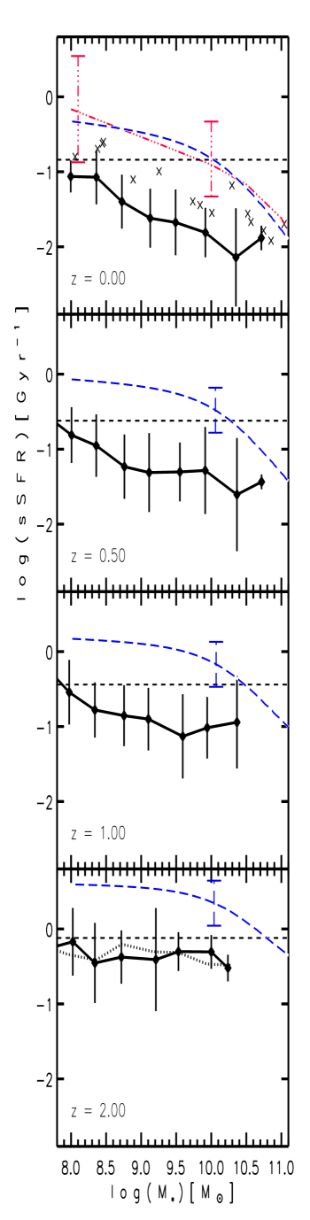
Figure 1: sSFR versus $M_{*}$ for s230 at $z=0,0.5,1$ and $2$. The mean relation and $1\sigma$ population scatter are shown with black solid lines. The horizontal short-dashed lines indicate the sSFR at the given epoch corresponding to the case of constant SFR: galaxies much above (much below) these lines are in a current active (passive) SF phase. The blue dashed curves correspond to results of an evolutionary toy model constrained to fit the empirical sSFR-$M_{*}$ and $F_{*}$–$M_{\rm vir}$ relations (see Appendix). At $z=0$, a fit to the observational results of Salim et al. (2007) and its scatter is shown with a red triple-dot-dashed curve. The crosses depict a subsample of galaxies with high sSFRs in more agreement with observations (see Section 3.3 for a detailed discussion). The black dotted line at $z=2$ denotes the results obtained by using the s320 simulation.

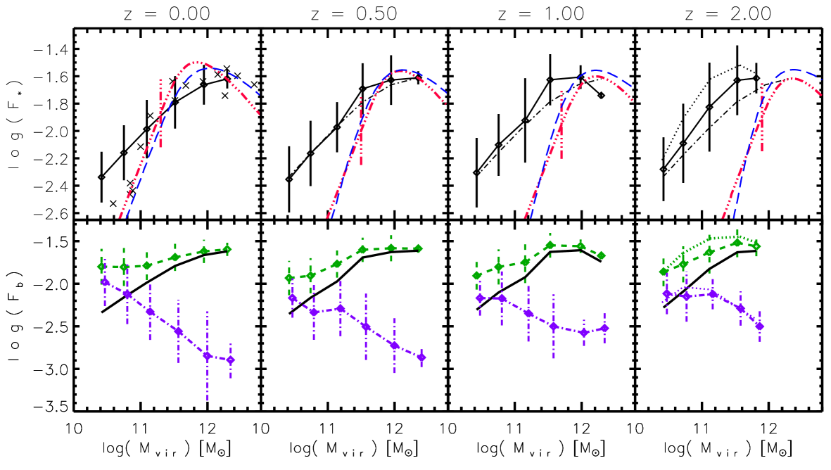
Figure 2: Upper panels: $F_{*}$ versus $M_{\rm vir}$ for s230. The mean relation and $1\sigma$ population scatter are shown at $z=0,0.5,1$ and $2$ (black solid lines). Results at $z=0$ are reproduced at higher $z$ for comparison (dot-dashed lines). The red triple-dot-dashed curves represent semi-empirical inferences and their $1\sigma$ uncertainty, while the blue dashed curves (shown also in Fig. 1) correspond to the toy model constrained to fit the empirical sSFR-$M_{*}$ and $F_{*}$–$M_{\rm vir}$ relations (see Appendix). The crosses depict the same high-sSFR galaxies showed in Fig. 1. Bottom panels: Mean $F_{b}$–$M_{\rm vir}$ (green dashed lines) and $F_{g}$–$M_{\rm vir}$ (violet dot-dashed lines) relations together with the corresponding standard deviations. For comparison, the $F_{*}$–$M_{\rm vir}$ curves are reproduced also in bottom panels (black solid curves). At $z=2$, the dotted lines in each panel represent the results obtained for $F_{*}$ (black, upper panel), $F_{b}$ (green, lower panel) and $F_{g}$ (violet, lower panel) by using the high resolution s320 simulation.

Figure 1 shows the sSFR of simulated galaxies averaged in bins of log$M_{*}$ versus the averaged log$M_{*}$ value of each bin. Vertical lines depict the standard deviation around the mean in each mass bin for the whole sample. The horizontal short-dashed line in each panel shows the sSFR that a galaxy would have if it had formed its stellar component at a constant SFR; in this case sSFR $\equiv$ SFR/$M_{*}$= 1/[(1 – R)($t_{H}$($z$) – 1 Gyr)], where $R=0.45$ is the assumed average gas return factor due to stellar mass loss, $t_{H}$ is the cosmic time, and 1 Gyr is subtracted to take into account the onset of galaxy formation.

In Fig. 1, the following trends can be appreciated: (a) simulated galaxies exhibit a tight relation between sSFR and $M_{*}$ at all epochs (the standard deviation is $\approx 0.3$ dex at $z=0$ and it does not increase significantly at higher $z$ for any of the mass bins); (b) the sSFR tends to decrease with $M_{*}$ in such a way that the relation becomes flatter at higher $z$ (by performing a linear fit in the log-log plane, the slope obtained for the relation is $\approx-0.40,-0.28,-0.20,$ and $-0.06$ at $z=0$, 0.5, 1.0 and 2.0, respectively); (c) the mean sSFRs of simulated galaxies are lower than those corresponding to the case of constant SFR since $z\sim 2$ (horizontal short-dashed lines; for $z>2$, galaxies tend to have a sSFR close to the case of constant SFR) being this difference larger for more-massive systems as $z$ decreases; (d) the average overall sSFR of the simulated galaxy population decreases significantly as $z$ decreases, roughly by a factor of $\sim 10-15$ from $z=2$ to $z=0$; the cosmic SFR in the entire box decreases by factor of $\sim 8$ during the same period.

We separate spheroid-dominated from disc-dominated galaxies by defining the latter as those systems with more than 75% of their gas component on a rotationally supported disc structure by using the condition $\sigma/V<1$ to select them. For more details, see de Rossi, Tissera & Pedrosa (2010) and De Rossi, Tissera & Pedrosa (2012). All the other systems are considered to be spheroid-dominated. We did not find a significant difference between the mean sSFR-$M_{*}$ relations of both groups. We have also separated central galaxies from satellites, and found that satellites exhibit a wider distribution of sSFRs than central systems. If any, the former systems have slightly larger sSFRs than the latter at a given $M_{*}$ for $z\mathchar 13358\relax 1$. The fraction of satellite galaxies in our simulation is actually small (0.21, 0.14, 0.13, and 0.12 at $z=0.0$, 0.5, 1.0 and 2.0, respectively), so that they hardly contribute to the mean sSFR-$M_{*}$ relation. The number of small satellites is determined by numerical resolution.

The blue dashed curves in Fig. 1 denote fittings to observations derived from a parametric toy model (for a compilation of observations and their comparison with these fits, see Fig. 11 in the Appendix). Simulated galaxies exhibit lower mean sSFRs than those derived from observations, being the difference larger as $z$ decreases . Moreover, most of simulated galaxies present sSFRs below the line associated to a constant SFR (black short-dashed lines). The deviations from the case of constant SFR increase with stellar mass and decrease with redshift, suggesting that the active phases of SF in simulated galaxies took place early, $z>1$. Nevertheless, as noted before, the simulations seem to be able to reproduce qualitatively the observed increase of sSFR for less-massive systems at low redshifts (downsizing in sSFR) and are also able to predict the flattening of the sSFR–$M_{*}$ correlation at higher redshifts. We will see that our SF and SN-feedback scheme in a multi-phase ISM plays a crucial role on generating these trends.

3.2 Stellar and baryonic mass fractions

In Figure 2, we can appreciate the dependences of $F_{*}$ (upper panels), $F_{b}$ and a similar defined fraction for the gas-phase, $\mbox{$F_{g}$}\equiv\mbox{$M_{g}$}/\mbox{$M_{\rm vir}$}$ (bottom panels) on $M_{\rm vir}$. Results are shown for the same four redshifts represented in Fig. 1.

The main trends obtained for $F_{*}$ (upper panels) can be summarised as follows: (a) $F_{*}$ systematically increases with $M_{\rm vir}$ at all available $z$, though, for our most massive galaxies, evidence of reaching a maximum at $\mbox{$M_{\rm vir}$}\sim 10^{12}$ $M_{\odot}$ is seen; (b) even at this maximum, the mean values of $F_{*}$ are not larger than $0.025$; (c) at $\mbox{$M_{\rm vir}$}\mathchar 13358\relax 10^{11}$ $M_{\odot}$, the $F_{*}$–$M_{\rm vir}$ correlation does not evolve significantly since $z\sim 2$ (roughly $\mbox{$F_{*}$}\propto M_{\rm vir}^{0.45}$) while, at $\mbox{$M_{\rm vir}$}\mathchar 13350\relax 10^{11}$ $M_{\odot}$, it becomes slightly steeper as $z$ increases; and (d) the scatter around the $F_{*}$–$M_{\rm vir}$ correlation is $\approx 0.2-0.3$ dex at $z=0$, increasing towards higher $z$.

The red triple-dot-dashed curves in the upper panels show the average $F_{*}$–$M_{\rm vir}$ correlations inferred by matching the observed GSMFs to the halo/subhalo mass functions. As described in FA10, results were obtained by parametrising a continuous function according to the data reported in Behroozi, Conroy & Wechsler (2010) in the separate redshift ranges $0\mathchar 13358\relax z\mathchar 13358\relax 1$ and $1\mathchar 13358\relax z\mathchar 13358\relax 4$. The error bar in each panel depicts an estimate of the uncertainties, which are mainly dominated by the systematic uncertainty in the determination of $M_{*}$ (Behroozi, Conroy & Wechsler, 2010). We can appreciate that the slope of the semi-empirical $F_{*}$–$M_{\rm vir}$ relation tends to be steeper than the simulated one since $z\sim 2$. In particular, simulated results at $z=0$ are close to those associated to the semi-empirical constraints at $\mbox{$M_{\rm vir}$}\mathchar 13350\relax 10^{11}$ $M_{\odot}$, deviating towards greater $F_{*}$ at the low-mass end of the relation. Note, however, that the latter differences should be smaller if the semi-empirical approach used a halo mass function derived from simulations that include baryons (see the footnote). Regarding the evolution with redshift, the semi-empirically inferred relation shifts systematically towards larger $M_{\rm vir}$ as $z$ increases, while the simulated relation exhibit negligible variations since $z\sim 2$. We do not find significant differences between the $F_{*}$–$M_{\rm vir}$ correlations associated to disc-dominated and spheroid-dominated systems.

In the bottom panels of Fig. 2, we analyse the evolution of $F_{b}$ and $F_{g}$. As $M_{\rm vir}$ decreases, $F_{b}$ significantly increases with respect to $F_{*}$, indicating the presence of higher gas fractions in the case of less-massive galaxies. As a result, the predicted $F_{b}$–$M_{\rm vir}$ correlations are much flatter than the $F_{*}$–$M_{\rm vir}$ ones, specially at lower $z$ (in the bottom panels, the $F_{*}$–$M_{\rm vir}$ correlations are reproduced again with black solid curves for comparison). $F_{b}$ reaches the maximum values in the case of most massive halos ($\sim 2\times 10^{12}$ $M_{\odot}$), with $\mbox{$F_{b}$}\approx 0.025-0.030$. The latter values are much smaller than the universal baryon fraction ($F_{b,U}$=0.15, for the cosmology adopted here), suggesting that significant outflow events may have affected these systems (see also de Rossi, Tissera & Pedrosa, 2010). Note that we consider the whole (cold + hot) gas component in our analysis. Nevertheless, for most simulated galaxies, more than 90% of the gas mass inside $R_{\rm bar}$ is cold ($T<15000$ K). The fraction of gas in the hot phase does not attain more than $\sim 20\%$ of $F_{g}$ for any of the systems, with the greater values associated only to most massive galaxies at $z=0$.

Regarding the evolution of the $F_{g}$–$M_{\rm vir}$ correlation (violet dotted-dashed lines), we can appreciate that since $z\sim 2$: for halos with $\mbox{$M_{\rm vir}$}\mathchar 13350\relax 5\times 10^{10}$ $M_{\odot}$, $F_{g}$ decreases with time, while for less massive halos, it systematically increases. At $\mbox{$M_{\rm vir}$}\sim 5\times 10^{10}$ $M_{\odot}$, $<\mbox{$F_{g}$}>\approx<\mbox{$F_{*}$}>\approx 0.008$ (i.e. $\mbox{$M_{g}$}/\mbox{$M_{*}$}\sim 1$). The increase of $F_{g}$ in the case of low-mass galaxies suggests that they have lower star formation efficiencies.

Finally, in Fig. 3, we analyse the galaxy gas mass fraction ($\mbox{$f_{g}$}\equiv\mbox{$M_{g}$}/\mbox{$M_{b}$}$) as a function of $M_{*}$ at $z=0,1$, and 2. Though the scatter is large, the simulations are able to reproduce at all epochs the observed trend of decreasing $f_{g}$ with $M_{*}$. The relation becomes slightly steeper as $z$ decreases in such a way that less-massive galaxies exhibit higher $f_{g}$ towards $z\sim 0$. Fig. 3 also shows results from a generalized analytical fit to the observed cold $f_{g}$-$M_{*}$ relation (Stewart et al., 2009). We see that, at a given $M_{*}$, observed (cold) gas fractions tend to be higher than those obtained for simulated galaxies, where most of the gas is actually in the cold phase. This is consistent with the fact that the sSFRs of the simulated systems are lower than observed ones (Fig. 1): simulated galaxies seem to have less cold gas available to fuel SF and more significant stellar mass fractions than observed galaxies.

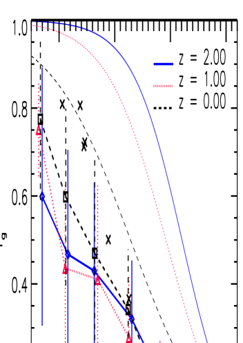
Figure 3: Average galaxy gas fraction vs $M_{*}$ at $z=2,1,0$ (blue solid, red dotted and black dashed lines, respectively). The error bars depict the $1\sigma$ population scatter. The dotted curves without error bars correspond to analytical fits to observations given in Stewart et al. (2009). Crosses denote results for the same galaxies with high-sSFR shown in Fig. 1.

3.3 Simulated galaxies in agreement with observations

In Fig. 1, we present the $\sim 7\%$ of galaxies with the highest sSFRs at $z=0$, which have gas fractions similar to those reported by observers. All these galaxies have sSFRs within the $1\sigma$ scatter associated to observations along almost three orders of magnitude in $M_{*}$, though slightly below the average observed values. The $F_{*}$–$M_{\rm vir}$ and $f_{g}$–$M_{*}$ relations for these galaxies at $z=0$ are also in general agreement with observations (Figs. 2 and 3, respectively). Therefore, our simulations were able to produce at least 15 galaxies that are within the scatters of the observational correlations studied here, while actually the average relations of the whole population significantly deviate from observed ones. Taken into account that these 15 systems are above the $1.5\sigma$ of the simulated distribution, these findings shows the relevance of studying the behaviour of the whole population in order to draw generic conclusions about average correlations of galaxies. Nevertheless, it is encouraging that simulations can generate some systems which have similar properties to observed galaxies in the Local universe.

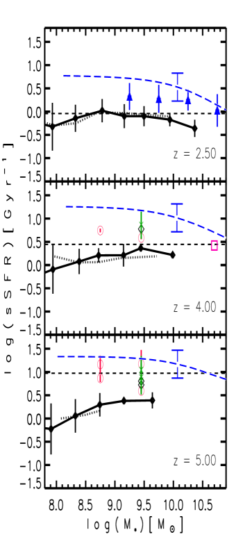
Figure 4: sSFR versus $M_{*}$ for the high-resolution s320 simulation at $z=2.5,4.0$ and $5$. See Fig. 1 for results at lower redshifts. The mean relation and $1\sigma$ population scatter are shown with black solid lines. The dotted lines show results in the case of s230 for comparison. The horizontal short-dashed lines indicate the sSFR at the given epoch corresponding to the case of constant SFR. Results from different observational works are shown: Bauer et al. (2011, blue triangles), Stark et al. (2013, green crosses), Gonzalez et al. (2012, red circles), Bouwens et al. (2012, black diamonds) and Daddi et al. (2009, pink square). The last three set of data correspond to star-forming galaxies. The blue dashed curves correspond to results of the evolutionary toy model (see Appendix).

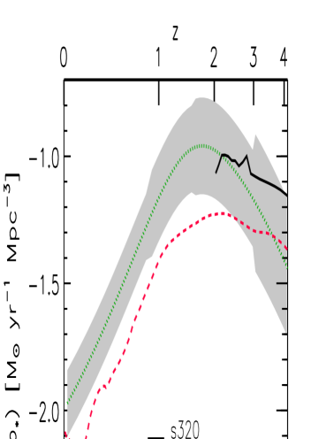
Figure 5: Cosmic SFR evolution for s230 (red dashed line) and s320 (black solid line; available only at $z\geq 2$). The green dotted line and shaded area depict the mean relation and standard deviations corresponding to a fit to compiled observations given in Behroozi, Wechsler & Conroy (2013).

3.4 Simulated galaxies at very high redshifts

In the case of s230, a significant fraction of galaxies have $N_{\rm sub}<2000$ at $z>2$. Instead, for s320 (available at $z\geq 2$), galaxies are yet well resolved since $z\sim 5-6$. Therefore, we employed the latter simulation for exploring the overall evolutionary trends of galaxies at very high redshifts and compared the results with the scarce available observational data (at $z>2$, most of observational studies are complete only for $\mbox{$M_{*}$}>5\times 10^{9}$ $M_{\odot}$).

Fig. 4 shows the sSFR as a function of $M_{*}$ at $z=2.5,4.0$ and 5.0 (see Fig. 1 for comparing these findings with results at lower redshifts). The black solid lines with error bars denote the mean relation and standard deviations corresponding to simulated galaxies in s320. Results obtained by using the s230 run are shown with dotted lines for comparison. The dashed horizontal lines indicate the case of constant SFR history ($R=0.30$ has been used for these early times). Findings from different observational works are also shown: Bauer et al. (2011, blue triangles), Stark et al. (2013, green crosses), Gonzalez et al. (2012, red circles), Bouwens et al. (2012, black diamonds) and Daddi et al. (2009, pink square). The last three set of data correspond to star-forming galaxies. We can see that, along the mass range where simulations and observations can be compared, the former are somewhat below the latter.

Figure 5 shows the cosmic SFR history in our simulated box for s320 (black solid line) as well as for s230 (red dashed line). The green dotted line and shaded area depict the mean relation and standard deviations corresponding to a compilation of observations given in Behroozi, Wechsler & Conroy (2013). The peak of the cosmic SFR is attained at $z\sim 2$, both in s320 and s230. Results from the high-resolution s320 run are in rough agreement with observations since $z\sim 5$ up to $z=2$. At higher $z$, the simulated cosmic SFR tends to be larger than what observations suggest, indicating that the gas is efficiently transformed into stars at very early times. However, the percentage of stellar mass assembled in this short time period is small with respect to the mass assembled at later epochs.

Finally, as the $M_{*}$–$M_{\rm vir}$ relations are poorly observationally constrained at high $z$, we present here the number density (per unit of comoving volume) of galaxies with log($M_{*}$/$M_{\odot}$)$=9.5\pm 0.25$ ($N_{\rm 9.5}$, black solid line in Fig. 6) as a function of $z$. Note that these galaxies have the largest masses in our box at these early epochs. A few observational studies were able to determine galaxy abundances down to these masses at high $z$. We plot some of such abundances in Fig. 6, using in all cases $h=0.7$. The simulated $N_{\rm 9.5}$ follows the same trend with z than observations, though with larger values. This is consistent with the high simulated $F_{*}$ obtained for the s230 run at $z\sim 1-2$ with respect to the semi-empirical determinations (Fig. 2). The fact that the number density of the largest simulated galaxies is already close to that derived from observations at these high $z$ indicates that the trend of assembling stellar mass earlier than empirical inferences is systematically stronger for smaller systems.

After the submission of this paper, a similar analysis was performed at $z\geq 2$ by using a cosmological hydrodynamical simulation in a box of $114^{3}$ Mpc³ side-lenght (Kannan et al., 2013). The simulated volume used by these authors is larger than the corresponding to s320 but the resolution is much lower. In spite of these differences, the trend and evolution predicted for the sSFR–$M_{*}$ relation, the GSMF and the cosmic SFR history are consistent with those reported here at $2\leq z\leq 5$, at least in the mass range where comparison is possible. We note that, at $z>2.5$, $N_{\rm 9.5}$ tends to be slightly lower in the the case of Kannan et al. (2013) than what the s320 run suggests (by $\sim 0.2-0.3$ dex), being these differences smaller when using the s230 run. However, at $1\times 10^{11}\mbox{$M_{\odot}$}<\mbox{$M_{\rm vir}$}\ <3\times 10^{11}$ $M_{\odot}$, their stellar mass fractions are lower than the ones obtained here by $\approx 0.7$ and $\approx 0.5$ dex at $z=2$ and $z=4$, respectively. These differences may be partially caused by the lower GSMF and $N_{\rm 9.5}$ abundances reported by Kannan et al. (2013), but it is also important to consider that the virial masses of our halos become smaller at higher $z$, than those measured in pure dark matter large simulations, showing a delay in their mass assembly (see also the upper panel of Fig. 7). The latter trend could be due to an environmental effect associated to our smaller volume. In spite of these issues, we find that the main evolutionary features of our low-mass galaxies at $z\geq 2$ are similar to those reported in Kannan et al. (2013).

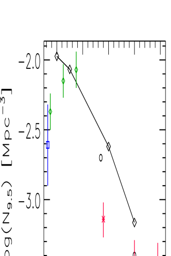
Figure 6: Number density (per unit of comoving volume) of galaxies with masses log($M_{*}$/$M_{\odot}$)$=9.5\pm 0.25$ as a function of redshift for s320 (black solid line). Observational measures are also shown: Marchesini et al. (2009, blue square), Mortlock et al. (2011, green diamonds), González et al. (2011, red asterisks), and Lee et al. (2012, black circles).

4 The mass assembly histories of galaxies and their halos

In this Section, we analyse the evolution of individual simulated systems selected from s230 according to their present-day mass with the aim of exploring their assembly histories since $z=2$. We focus only on those central galaxies with $\mbox{$M_{\rm vir}$}\ \mathchar 13350\relax 10^{10.3}M_{\odot}$ at $z=0$ ($N_{\rm sub}>2000$) and follow the evolution of their main progenitors back in time. In order to determine reliable evolutionary trends, when reconstructing the evolutionary histories, we consider that all the substructures identified in the simulated box ($N_{\rm sub}\geq 20$) are plausible progenitors.

4.1 Galaxy vs halo mass assembly

In the left panels of Fig. 7, we can appreciate the average virial halo, galaxy stellar, and galaxy baryonic MAHs for four different subsamples of galaxies defined at $z=0$ according to their log($M_{\rm vir}$/$M_{\odot}$): $<10.5,10.5-11.0,11.0-11.5,$ and $\geq 11.5$. The error bars correspond to the standard deviations associated to each subsample at a given $z$. To avoid overplotting, the means and error bars are slightly shifted along the horizontal axis and the error bars are not shown at all epochs. The right panels portray the same information but the MAHs were normalized to the corresponding present-day masses in order to get more insight into the shape of the evolutionary tracks and its dependence on mass. For the sake of clarity, only the lowest and highest mass bins are shown in right panels (galaxies in the other bins exhibit an intermediate behaviour).

In the upper panels, for comparison, we also show the mean halo MAHs from the Millennium simulations as fitted by Fakhouri, Ma & Boylan-Kolchin (2010, dotted lines) and corresponding to the present-day masses shown for our simulations. We obtain a general good agreement taking into account that our box is much smaller than those of the Millennium simulations and that those simulations include only collisionless (dark) matter. Systematic differences can be appreciated at $z>1$, implying a slightly later mass assembly in s230 than in the case of the Millennium simulations. These differences are more pronounced for smaller masses, which suffer more dramatic SN-driven outflows, specially at earlier epochs. Although with a large scatter, for both the Millennium simulations and s230, more massive systems tend to assemble their virial masses typically later than the less massive ones (hierarchical mass assembly or upsizing). However, in the case of s230, this trend is weaker, mainly due to the later assembly of simulated low-mass systems. For instance, for the smallest mass bin at $\log(\mbox{$M_{\rm vir}$}/\mbox{$M_{\odot}$})<10.5$, the redshift at which $M_{\rm vir}$ attains 50% of its present-day value is $z_{\rm h,1/2}\approx 1.35$ (ranging from $z\approx 0.75$ to 1.81 for the 1$\sigma$ population), while at $\log(\mbox{$M_{\rm vir}$}/\mbox{$M_{\odot}$})\geq 11.5$, $z_{\rm h,1/2}\approx 1.16$ (ranging from $z\approx 0.80$ to 1.60 for the 1$\sigma$ population).

The solid lines in the middle panels show the average galaxy stellar MAHs. The slight upsizing trend with mass for the halo MAHs is reversed to a downsizing trend in the case of the stellar MAHs: galaxies in less massive halos assemble their present-day $M_{*}$ slightly later than those in more massive ones, though the scatter is large. This trend can be better appreciated in the case of the normalized stellar MAHs ($M_{*}$($z$)/$M_{*}$($z=0$)). For the same two extreme ranges of virial masses mentioned above, $\log(\mbox{$M_{\rm vir}$}/\mbox{$M_{\odot}$})<10.5$ and $\log(\mbox{$M_{\rm vir}$}/\mbox{$M_{\odot}$})\geq 11.5$, the redshifts at which $M_{*}$ attains 50% of its present-day value are $z_{\rm s,1/2}\approx 0.80$ (ranging from $z\approx 0.4$ to 1.4 for the 1$\sigma$ population) and $z_{\rm s,1/2}\approx 1.30$ (ranging from $z\approx 0.8$ to 1.7 for the 1$\sigma$ population), respectively. Hence, simulations seem to be successful in predicting the observed downsizing trend for $M_{*}$, albeit the tendency is weak.

Figure 7: Average halo (top panels), galaxy stellar (middle panels), and galaxy baryonic (bottom panels) mass aggregation histories for four $\log(\mbox{$M_{\rm vir}$}/M_{\odot})$ bins defined at $z=0$ (solid lines): $<10.5$ (red diamonds), $10.5-11$ (black triangles), $11-11.5$ (pink squares) and $\geq 11.5$ (blue crosses). In the left panels, the average value of the progenitor mass at a given redshift is calculated for each bin. In the right panels, the averages in each bin are calculated considering the mass of each galaxy at a given redshift normalized to its final value at $z=0$. For the sake of clarity, only the lowest and highest mass bins are shown in right panels (galaxies in the other bins exhibit an intermediate behaviour). Error bars represent $1\sigma$ population scatter. In the case of the halo MAHs, the dotted lines show the results derived from eq. (2) of Fakhouri, Ma & Boylan-Kolchin (2010). In the case of the stellar and baryonic components, together with the evolution of galaxy masses inside $R_{\rm bar}$, the corresponding evolution of masses inside the whole halo, up to $R_{\rm vir}$, are also plotted (short-dashed curves). The dotted curves in the medium left panel corresponds to inferences from a toy parametric model constrained to fit observations (see Sect. 4.4 and Appendix) and are associated to the same four mass bins used for the simulations, with $\log(\mbox{$M_{\rm vir}$}/M_{\odot})$ increasing from the lower to the upper dotted curve.

The galaxy baryonic MAHs do not differ significantly from stellar ones (lower panels of Fig. 7). The downsizing trend obtained for $M_{*}$ can be also appreciated in the case of $M_{b}$. However, differences in the absolute values are evident: while for the least massive systems, $M_{b}$ is significantly larger than $M_{*}$ at all available $z$ (roughly a factor of $\sim 3$), for the most massive ones, $M_{b}$ is only slightly larger than $M_{*}$, being this difference somewhat larger at higher redshifts. The mentioned trends are explicitly seen in Fig. 8, where the mean evolution of $f_{g}$ is plotted for our simulated galaxies grouped according to their present-day halo masses. As expected, less massive galaxies exhibit high percentages of gas at all epochs while in the case of larger systems, $f_{g}$ significantly decreases towards $z\sim 0$.

4.2 Assembly of stars and gas inside virialized halos

We can appreciate the MAHs for the whole stellar and baryonic components inside $R_{\rm vir}$ in the middle and lower panels of Fig. 7, respectively (dashed lines). In the case of $M_{*}^{\rm vir}$, the mass fraction outside the central galaxy can be found in satellite galaxies and also in an extended stellar halo. For massive halos, this fraction is small and it slightly increases with $z$ from $\approx 20\%$ at $z\sim 0$ to $\approx 35\%$ at $z>2$. In the case of smaller halos, the stellar component outside central galaxies was significant at high $z$, decreasing towards lower $z$.

Regarding the whole baryonic component, $M_{b}^{\rm vir}$ seems to be significantly larger than the baryonic mass contained inside central galaxies at all epochs. These differences are higher in the case of less massive systems, in particular at high $z$. These results imply the presence of significant fractions of gas in simulated halos, with the greater percentages obtained for smaller systems and at higher $z$ (see also de Rossi, Tissera & Pedrosa, 2010). The MAHs represented by the evolutionary tracks of $M_{b}^{\rm vir}/M_{b}^{\rm vir}(z=0)$ (lower right panel) are quite diverse (large error bars) specially for small halos, where there is a significant interplay between gas (re)accretion and feedback-driven outflows. It is clear that $M_{b}^{\rm vir}$ in some small halos decreases towards $z\sim 0$, probably due to strong outflows (de Rossi, Tissera & Pedrosa, 2010). On average, the MAHs associated to $M_{b}^{\rm vir}$ seem to follow qualitatively the upsizing trend of the halo MAHs. However, less massive systems tend to assemble $M_{b}^{\rm vir}$ earlier than the corresponding $M_{\rm vir}$. These trends are probably caused by a very efficient SN feedback that avoids late gas capture by the galaxy and promotes gas ejection from the halos. Nevertheless, our findings suggest that a significant amount of gas resides inside these halos, probably supported by thermal pressure (hot-gas phase). Part of this gas may cool later leading to an increase of the SFR in the galaxy.

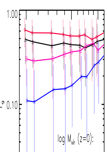
Figure 8: Evolution of the average gas fraction of simulated galaxies grouped into the same four halo mass bins defined at $z=0$ and shown in Fig. 7. Error bars represent the $1\sigma$ population scatter.

4.3 Evolution of the stellar and baryonic mass fractions

The evolution of the average $F_{*}$ and $F_{b}$ (solid lines) can be appreciated in Fig. 9 in the left and right panels, respectively. As in previous figures, the mean relations for four mass bins are shown, with the error bars denoting the associated standard deviations. In both panels, the short-dashed lines show the results obtained for the stellar ($F_{*}^{\rm vir}$) and baryonic ($F_{b}^{\rm vir}$) mass fractions measured inside $R_{\rm vir}$ (instead of $R_{\rm bar}$).

As can be seen, at all epochs, $F_{*}$ is systematically lower in galaxies formed in present-day low-mass halos than in galaxies formed in more massive halos. In fact, the evolution of $F_{*}$, though with a large scatter, is such that for low-mass galaxies, $F_{*}$ decreases towards higher $z$, while for more massive galaxies, $F_{*}$ does not change significantly up to $z\sim 2$ (for the most massive galaxies, $F_{*}$ can be a bit larger at higher $z$). These findings suggest that for massive galaxies ($\mbox{$M_{*}$}>10^{10}\mbox{$M_{\odot}$}$), $M_{*}$ tends to assemble at a similar rate than $M_{\rm vir}$, while for less-massive galaxies, $M_{*}$ assembles later than $M_{\rm vir}$. Regarding $F_{*}^{\rm vir}$ (dashed lines), we did not obtain systematic variations with $z$ for any of the considered mass bins, suggesting that the total stellar and dark matter components tend to increase at a similar rate inside $R_{\rm vir}$.

In the case of galaxies in massive halos, the evolutionary tracks of $F_{b}$ (right panel of Fig. 9, pink and blue curves) follow closely those obtained for $F_{*}$. For less massive halos, as noted before (see Figs. 3 and 8), the gas-phase tends to dominate the baryonic component of simulated galaxies, being $\mbox{$F_{b}$}>\mbox{$F_{*}$}$. In particular, for galaxies in the lowest-mass bins, $F_{b}$ is not only much higher than $F_{*}$ but it increases slightly faster than $F_{*}$ since $z\sim 1$, probably evidencing the re-infall of gas ejected from the systems at early times.

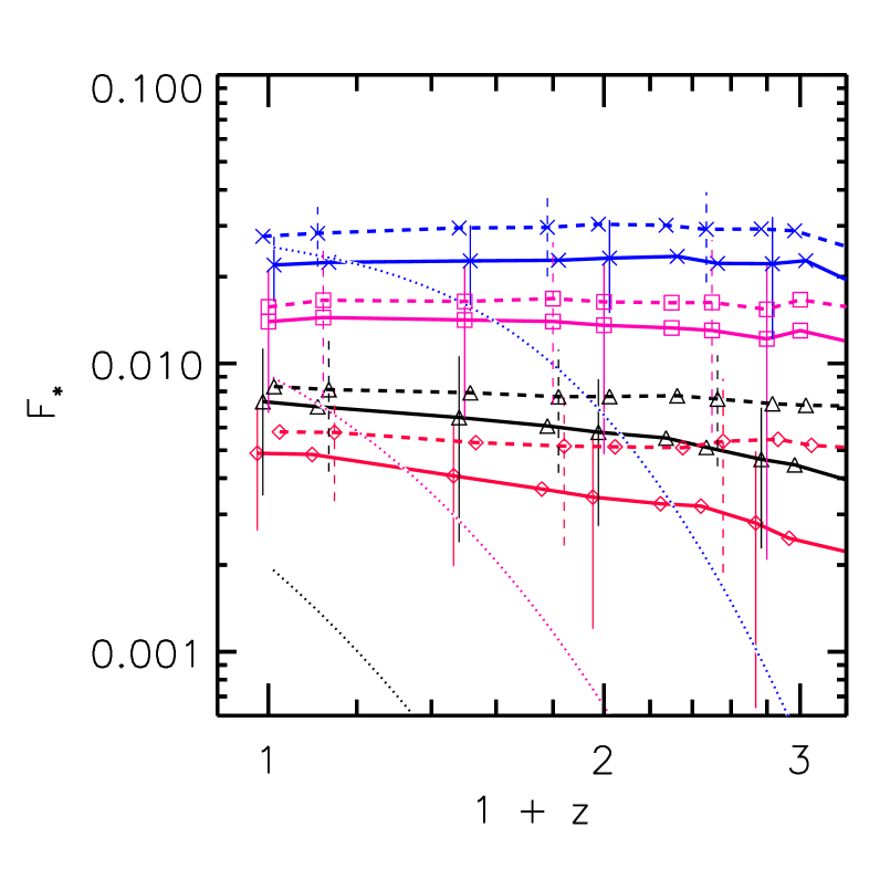
Figure 9: Evolution of the average galaxy stellar (left panel) and baryonic (right panel) mass fractions (solid lines) grouped into the same four halo mass bins defined at $z=0$ and shown in Fig. 7. Error bars represent the $1\sigma$ population scatter. The stellar and baryonic fractions obtained by considering the whole mass enclosed inside $R_{\rm vir}$ ($F_{*}^{\rm vir}$ and $F_{b}^{\rm vir}$, respectively) are represented with short-dashed lines. In the left panel, the dotted curves depict the inferences derived from the toy parametric model constrained to fit observations (see Sect. 4.4 and Appendix) and are associated to the same four mass bins used for the simulations, with $\log(\mbox{$M_{\rm vir}$}/M_{\odot})$ increasing from the lower to the upper dotted curve.

Regarding $F_{b}^{\rm vir}$, we do not detect systematically variations with $z$, on average. Therefore, the baryonic content inside $R_{\rm vir}$ follows roughly the MAH of the halo (specially in the case of the most massive bin), as discussed before. In fact, since a similar trend was also obtained for $F_{*}^{\rm vir}$, the different components (gas, stars and dark matter) inside $R_{\rm vir}$ seem to increase at the same rate in these simulations, at least since $z\sim 2$. On the other hand, the percentage of baryons (mainly gas) in the halos is of the order or larger than the baryonic fraction contained in the central galaxies. At $z=0$, for instance, the average $F_{b}^{\rm vir}$ is $\sim 2-2.5$ times larger than $F_{b}$ in the whole simulated mass range. Hence, outside the central galaxies there is, on average, an amount of mass similar or up to $\sim 1.5$ times the baryonic mass of these galaxies. In the case of the stellar component, $F_{*}^{\rm vir}$ is only up to $\sim 1.2$ times larger than $F_{*}$. Thus, most of the baryonic matter outside central galaxies is actually in the gas-phase. At higher redshifts, the differences between $F_{b}$ and $F_{b}^{\rm vir}$ increase for less-massive galaxies. At $z=3$, for example, galaxies residing in the lowest-mass present-day halos had $\sim 7$ times more baryons outside the galaxy than within it, being most of these baryons part of the hot-gas component.

Figure 10 summarises the evolution of $F_{*}$, $F_{*}^{\rm vir}$, $F_{b}$ and $F_{b}^{\rm vir}$ as a function of the present-day halo mass. In this case, the individual mass fractions were normalized to their present-day values before averaging over the different mass bins so that, the patterns associated to the different evolutionary histories can be more easily compared.

Results for $F_{*}$ are presented in the upper left panel. Although the scatter is large, the stellar MAH of galaxies is clearly dependent on $M_{\rm vir}$: as the mass of galaxies decreases, the stellar component tend to assembles later than the halo. For the smallest systems, $F_{*}$ increases, on average, by a factor of $\sim 2$ since $z\sim 2$ to $z\sim 0$, while for the largest ones, $F_{*}$ does not change significantly or slightly decreases with time in some cases. Hence, for more massive systems, the stellar MAHs seem to follow closely the MAHs of the halos. In the lower left panel, we can appreciate the evolution of $F_{*}^{\rm vir}$. As can be seen, for the whole component inside $R_{\rm vir}$, the patterns associated to the mean evolution of the stellar-to-halo mass ratio are approximately scale-independent, exhibiting also no significant evolution since $z\sim 2$.

According to the right panels of Fig. 10, the baryonic-to-halo MAHs of galaxies seem to be dependent on scale but with a much larger scatter than the one obtained for the stellar-to-halo MAHs. For the smallest systems, the average $F_{b}$ increases by less than a factor of $\sim 2$ since $z\sim 2$ while for the largest ones, $F_{b}$ does not change significantly or slightly decreases with time. In the case of $F_{b}^{\rm vir}$, though with a large scatter, its evolutionary history seems to show an opposite trend to the one obtained for $F_{*}$ or $F_{b}$: for galaxies with lower $M_{\rm vir}$, $F_{b}^{\rm vir}$ tends to exhibit a more significant decrease with time. These findings suggest that in these simulations, many low-mass halos tend to lose baryons with time, but we have seen that there is also a non-negligible percentage of low-mass systems that do not experience significant outflows and/or re-accrete baryons lately.

Figure 10: Evolution of the same stellar (left panels) and baryonic (right panels) mass fractions shown in Fig. 9 but normalized to their present-day values in such a way that the patterns of the mass-dependent evolutionary tracks can be more easily compared. Error bars show the corresponding standard deviations. The upper panels show results for galaxy masses enclosed by $R_{\rm bar}$, while lower panels correspond to total masses inside $R_{\rm vir}$. The averages were derived considering the mass fraction of each galaxy at a given $z$ normalized to its value at $z=0$. In the upper left panel, the dotted curves indicate the inferences from the toy parametric model constrained to fit observations (see Sect. 4.4 and Appendix) and are associated to the same four mass bins used for the simulations, with $\log(\mbox{$M_{\rm vir}$}/M_{\odot})$ increasing from the lower to the upper dotted curve.

4.4 Comparison with empirical inferences

With the aim of comparing the average MAHs derived from simulations and empirical inferences, we use a simple toy parametric model of the average halo and stellar mass growth constrained by observations (González-Samaniego & Avila-Reese, 2012, see the Appendix for a more detailed description). In this toy model, the average evolution of $M_{*}$ inside the growing halos describes, by construction, the empirical sSFR–$M_{*}$ and $F_{*}$–$M_{\rm vir}$ mean relations at different redshifts, which can be considered isochrones of the evolutionary tracks. As discussed in the Appendix, the increase of $M_{*}$ is driven mainly by in-situ SF but, in order to obtain agreement with the empirical relations, a small contribution of ex-situ stellar mass acquisition (dry mergers) is necessary for high masses. It is worth noting that this toy model does not attempt to include physical prescriptions for the evolution of baryons; it is just constrained to reproduce observations. Similar approaches were presented previously in the literature (FA10, Conroy & Wechsler, 2009; Leitner, 2012) and, in all cases, the most general trends are consistent to the ones derived from our toy model. Furthermore, these trends are in good agreement, at the masses and redshifts when a comparison is possible, with archaeological inferences (see the Appendix). In Sec. 3, the results of this toy model were used as descriptions of observations and compared with the predictions of our numerical simulation. In this section, we will extend this comparison to the average MAHs of galaxies.

As shown before, in the left middle panel of Fig. 7, we can appreciate the toy model tracks associated to $M_{*}$ (dotted lines) for galaxies with present-day log($M_{\rm vir}$/$M_{\odot}$) = 10.30, 10.75, 11.25, and 11.75 (from bottom to top), which are representative of the mass bins used in the simulations. As the mass decreases, the stellar MAHs of simulated galaxies exhibit more significant deviations from the toy model tracks. As anticipated, in the simulations, $M_{*}$ tends to assemble earlier than what the toy model indicates, being the difference systematically larger for lower masses. Regarding the halo mass assembly, the toy model is based on the mass aggregation rates given in Fakhouri, Ma & Boylan-Kolchin (2010), which are shown with dotted curves in the upper panels of Fig. 7.

It should be noted that the toy model is constrained by observations only above $\sim 10^{9}$ $M_{\odot}$ and the lowest-mass tracks are actually extrapolations. Studies of the past SF history of relatively isolated nearby dwarf galaxies by means of color-magnitude diagrams obtained with the Hubble Space Telescope (HST) show that low-mass systems (specially below $\sim 10^{8}$ $M_{\odot}$) typically assembled most of their stars at $z>1-2$ (Weisz et al., 2011). The present-day sSFR of these field dwarfs seems to be lower than the extrapolation to lower masses of the trends in Salim et al. (2007, Fig. 1). On the other hand, studies based on UV analysis, assign systematically higher SFRs to dwarf galaxies, in better agreement with Salim et al. (2007, e.g., , ). Above $\sim 10^{8}$ $M_{\odot}$, as the mass decreases, the stellar mass assembly is systematically delayed. On the contrary, below $\sim 10^{8}$ $M_{\odot}$, this trend seems to be interrupted, with the stellar component of small galaxies commonly assembling very early (Leitner, 2012). Therefore, the evolutionary tracks inferred with our toy model should be taken with caution at $M_{*}$ below $10^{8}$ $M_{\odot}$ (lowest dotted line in Figs. 7, 9, and 10).

In the left panels of Figs. 9 and 10, we can appreciate that the evolution of $F_{*}$ inferred with the toy model deviates from the one predicted by the simulations. As the mass decreases, the toy model suggests a more significant delay in the stellar mass assembly with respect to the halo one. For galaxies in halos with present-day masses of $\sim 10^{12}$ $M_{\odot}$, the stellar mass fractions associated to the toy model decrease $\sim 3$ times more towards $z\sim 1$ than what simulations suggest, while this difference increases roughly up to 20 times for galaxies in halos of $3-10\,\times 10^{10}$ $M_{\odot}$ (compare the corresponding dotted and solid curves in Fig. 10). Part of this discrepancy is caused by the different halo MAHs associated to the toy model and the simulations: the simulated $M_{\rm vir}$ decays faster with $z$ than the dark matter MAHs given in Fakhouri, Ma & Boylan-Kolchin (2010, see Fig. 7).

The delay in the stellar mass assembly of smaller galaxies could also depend on the observational data used to constrain the toy model. In particular, Yang et al. (2012) have recently reported new inferences regarding the evolution of the $M_{*}$–$M_{\rm vir}$ relation: for one of the cases analysed by those authors at low masses, at a given $M_{\rm vir}$, $M_{*}$ decreases faster than what the $M_{*}$($M_{\rm vir}$,$z$) function given by FA10 implies. In our toy model, the tracks that would fit the $M_{*}$($M_{\rm vir}$,$z$) function reported by Yang et al. (2012) lead to steep sSFR–$M_{*}$ relations at low masses. Thus, the delay in the $M_{*}$ growth of smaller galaxies could be even more dramatic than what we have discussed here. On the other hand, Behroozi, Wechsler & Conroy (2013) obtained new constraints on the $M_{*}$($M_{\rm vir}$,$z$) function. According to the latter work, the $M_{*}$($M_{\rm vir}$,$z$) function does not change significantly with $z$ in such a way that for smaller galaxies, the stellar mass growth is shallower than what we have inferred here, leading to a better agreement with our simulations but yet with differences.

Finally, although the trend is weak, it is encouraging that the SN feedback model used in this work is able to reverse the upsizing trend of the halo MAHs to a downsizing trend in the case of stellar MAHs. In the next section, we discuss about possible additional physical prescriptions that could be implemented in the simulations to tackle the issue of the early stellar mass assembly and obtain a better agreement with empirical inferences.

5 Discussion

As we mentioned in Sec. 1, this work does not attempt to analyse in detail the particular predictions of the subgrid model implemented in these simulations. We aim mainly to discuss about the general trends which are shared with other numerical works based on current models and simulations of structure formation. As discussed before, recent results obtained by re-simulating selected objects at high resolution (see Sec. 1) lead to reasonable consistency with observations. Although the resolution of our simulations is lower than in those studies, both approaches predict similar trends in general, with the advantage that our simulated sample include a larger number of systems. Hence, we are able to analyse statistically the evolutionary histories of galaxies covering a more significant dynamical range. Exhaustive explorations of different subgrid schemes and physical parameters were carried out recently in the literature, showing how the properties and evolution of simulated galaxies may change according to the subgrid assumptions (e.g., Saitoh et al., 2008; Colín et al., 2010; Davé, Oppenheimer & Finlator, 2011; Faucher-Giguère, Kereš & Ma, 2011; Hummels & Bryan, 2012; McCarthy et al., 2012; Scannapieco et al., 2012). The simulation analysed here is actually part of such studies, having been its subgrid physics and parameters chosen to produce nearly realistic galaxies in what regards global structural and dynamical properties (de Rossi, Tissera & Pedrosa, 2010; De Rossi, Tissera & Pedrosa, 2012).

5.1 Subgrid physics in the simulations

The modelisation of SF-driven outflows is crucial for reproducing the flattening of the GSMF at the low-mass end or, similarly, for predicting the decrease of $F_{*}$ for lower $M_{\rm vir}$. For example, Oppenheimer et al. (2010) showed how the GSMF changes according to different feedback models implemented in their TreeSPH GADGET-2 simulations. In all these models, the feedback is directly related to the SFR and is included as a kinetic energy added to gas particles. These particles are temporarily hydrodynamically decoupled in order to provide a low resistance avenue for SN feedback to escape out of the galaxy. Oppenheimer et al. (2010) found that the gas ejected and lately re-accreted by the galactic systems is a key mode of galaxy growth. If the gas acquired by the galaxies through this mode is artificially suppressed, then the (unrealistic) GSMFs obtained at $z=0$ are similar in spite that the feedback models are different. But, when taking into account the re-accreted gas, then the GSMF depends sensitively on it.

Oppenheimer et al. (2010) reported that a better agreement with the observed GSMF is obtained when rather than an ”energy-driven” wind, a ”momentum-driven” wind is introduced (Murray, Quataert & Thompson, 2005). However, the re-accretion mode is mass-dependent, increasing its efficiency as the mass increases (for massive galaxies, a local fountain effect is obtained). The parameters of the momentum-driven winds can be tuned to reproduce roughly the low- and intermediate-mass regions of the GSMF due to the late ($z\mathchar 13358\relax 2$) differential gas re-accretion. However, at the high-mass end, too massive galaxies are obtained because of the fast re-accretion exhibited during the evolutionary history of these galaxies.

These results are similar to those obtained by Firmani, Avila-Reese & Rodríguez-Puebla (2010) by means of disc galaxy evolutionary models in the context of the $\Lambda$CDM scenario. They showed that the $F_{*}$–$M_{\rm vir}$ relation (associated to the GSMF) at low and intermediate masses can be reproduced by the models when efficient momentum-driven outflows and differential re-accretion depending on the infall rate (environment) are included. However, the models in this case show a sSFR that increases with $M_{*}$, being close to present-day observations at intermediate masses ($\mbox{$M_{*}$}\sim 3-6\times 10^{10}$ $M_{\odot}$), but systematically lower than observations for lower $M_{*}$. This behaviour can be explained by the early mass loss and the decreasing efficiency of gas re-accretion for lower masses. The latter result has been also found by Davé, Oppenheimer & Finlator (2011), who used TreeSPH numerical simulations similar to those of Oppenheimer et al. (2010). These authors show that an outflow model following scales expected for momentum-driven winds broadly matches the observed galaxy evolution around $M^{\star}$ since $z=3$ to 0, but it fails at higher and lower masses.

The SN-driven feedback model implemented in our simulation is physically more self-consistent than those based on kinetic energy input and temporary hydrodynamical decoupling in the sense that the model is tied to a multi-phase treatment of the gas components in the ISM. Note that the energy injected by SNe to the gas particles is thermal and it depends on the thermodynamic properties of the particles. This energy can promote particles from the cold/dense phase to the hot/diffuse phase, influencing thus the SFR.

The SN feedback modelled in this way has therefore a relevant influence both locally, affecting the gas properties and the SFR, and globally, producing pressure-driven large-scale gas and metals outflows. The latter effect is the one that produces the flattening of the GSMF at the low-mass end or the decrease of $F_{*}$ for lower $M_{\rm vir}$ (see above). Note that this effect can also produce a systematic decrease of the sSFR at late epochs for lower masses because smaller galaxies lose more efficiently their gas and are less susceptible to re-accrete it lately (Firmani, Avila-Reese & Rodríguez-Puebla, 2010; Davé, Oppenheimer & Finlator, 2011). In this context, it is relevant to remark that in our simulation, the present-day sSFR does not decrease towards lower $M_{*}$ (Fig. 1), on the contrary, it increases with a slope close to observations. This success is due to the local effects of our thermal feedback model: a significant fraction of the left-over gas in small galaxies is maintained in a hot phase in the disc and halo, being able to cool lately and produce a sustained SF activity. According to Fig. 3, as the mass of simulated galaxies decreases, higher gas fractions are obtained. In addition, the large amounts of gas in the halos of small galaxies tend to decrease with time contributing to the increase of the galaxy stellar and gas mass fractions (see Fig. 9). For the largest galaxies, the gas in the halo does not exhibit significant variations with time.

All these findings are consistent with the presence of two different thermodynamic regimes in these simulations as described in detail by de Rossi, Tissera & Pedrosa (2010). In the case of smaller galaxies, the virial temperatures are lower and, therefore, SN heating is more efficient at promoting gas from the cold to the hot phase. However, the cooling times of these systems are shorter than the dynamical times and the hot gas can return to the cold phase on short time-scales. Therefore, for low-mass galaxies, SN feedback leads to a self-regulated cycle of heating and cooling strongly influencing the SF activity of these systems. In the case of massive galaxies, the hot phase is established at a higher temperature and, hence, SN heating cannot generate an efficient transition of the gas from the cold to the hot phase; meanwhile, the cold gas remains available for SF. In addition, the cooling times for larger galaxies get longer compared to the dynamical times and the hot gas is able to remain in the hot phase during longer time-scales. Hence, SN feedback is not efficient at regulating the SF in massive galaxies. As shown by de Rossi, Tissera & Pedrosa (2010), in this model, this transition from an efficient to an inefficient cooling regime for the hot-gas phase produces a bend of the stellar Tully-Fisher Relation in good agreement with observations.

In spite of this partial success, in Sec. 3 and 4.4, we have seen that the sSFR–$M_{*}$ and $F_{*}$–$M_{\rm vir}$ correlations, and the MAHs of the low-mass simulated galaxies still exhibit discrepancies with some observational inferences. Although in our simulation the upsizing trend of dark matter seems to be reverted to a downsizing trend in the case of stellar mass, this behaviour is still weaker than what observations suggest. In the next section, we discuss about different possibilities to tackle these issues.

5.2 What should be improved?

Would the increase of the feedback model efficiency help to solve the above-mentioned issues? The parameters of our feedback model were constrained to reproduce properties of MW sized galaxies (Scannapieco et al., 2008), being the typical outflow velocities generated in simulated galaxies consistent with observational inferences (Scannapieco et al., 2006, 2008). The fraction of SN energy and metals injected into the cold phase, $\epsilon_{c}=0.5$, could hardly be increased. As discussed in Sawala et al. (2011), for dwarf galaxies, this efficiency should be decreased in order to be consistent with the observed mass–metallicity relation. Moreover, the feedback-driven outflows seem to be very efficient in our simulation: halos that today are smaller than $\mbox{$M_{\rm vir}$}\sim 10^{11}$ $M_{\odot}$ have inside them only around 25% of the universal baryon fraction since $z\sim 2$, while the largest halos in our simulation ($\mbox{$M_{\rm vir}$}>3\times 10^{11}$ $M_{\odot}$) have also small baryonic fractions ($\approx 35-40$% of the universal one, see Fig 9).

In fact, the comparison with observational inferences shows that besides the increase of the ejected mass for smaller galaxies, a delay in the SF process is also necessary. A more complete treatment including multiple feedback processes on different scales could work in this direction. For instance, in addition to the SN wind shock heating, Hopkins, Quataert & Murray (2012) considered also the momentum deposition from radiation pressure, SNe, stellar winds, the photoheating of HII regions, and other processes. These authors show that the effects of all these feedback processes affect in different ways the galactic winds as well as the properties of the simulated galaxies, depending on their masses and SF regimes. On the other hand, Puchwein & Springel (2012) claim that by tuning appropriately the energy-driven kinetic feedback in their SPH simulations, the observed $F_{*}$–$M_{*}$ and sSFR–$M_{*}$ relations, and other properties could be reproduced. The key ingredients in their feedback model are the assumptions that the wind velocity depends on the galaxy potential well and that the loading factor is proportional to this velocity.

During the refereeing of this paper, a preprint by Aumer et al. (2013) appeared, where the authors discuss some improvements on the Scannapieco et al. (2008) subgrid physics used here. In the new proposed scheme, the effects of radiation pressure from massive young stars on the ISM are included, helping to reproduce disc galaxies with small bulges, sizes, star formation rates, among other properties, in global agreement with observations at $z=0-3$. For higher $z$, higher star formation efficiencies are still present, suggesting the need for new physical processes to be included.

Another avenue of exploration in simulations is related to the SF process. For example, Krumholz & Dekel (2012) and Kuhlen et al. (2012) have proposed that the formation of molecular gas, $H_{2}$, in galaxies could be delayed in low-mass/low-surface brightness galaxies because they have lower metallicities at earlier epochs. Only after a threshold metallicity and gas surface density are fulfilled, neutral hydrogen transforms efficiently into $H_{2}$ in the high-density, cold regions, being the smaller galaxies subject to this process at lower redshifts.

A recent SPH cosmological simulation of a dwarf galaxy that includes an explicit method for tracking the non-equilibrium abundance of $H_{2}$, shows that the dwarf has a larger gas fraction and higher SFR at later times than the simulation without the $H_{2}$ treatment (Christensen et al., 2012).

Finally, as discussed before, our results seem not to be significantly affected by resolution issues. When comparing results derived from s230 with those obtained for the higher-resolution simulation s320 (available only at $z\geq 2$), similar trends were found. In Figs. 1 and 2, the dotted lines at $z=2$ indicate the trends obtained by using s320. We can appreciate that the relations associated to s230 and s320 are very close. Galaxies in s320 seem to have been slightly more efficient in assembling their stellar component than systems in s230 but the differences are not significant. Even at higher redshifts ($z>2$), the trends exhibited by s230 remain very similar to those obtained for s320, though the small aforementiononed differences seem to be more evident at these $z$ (see Fig. 4). Regarding the cosmic SFR histories of both runs (Fig. 5), we see that, in general, s230 and s320 lead to similar trends exhibiting also no significant differences. These findings are consistent with the results of de Rossi, Tissera & Pedrosa (2010), who found that the dynamical properties of galaxies in s230 seem to be robust against numerical artefacts (the reader is referred to that paper for more details).

6 Conclusions

A whole population of low-mass galaxies was simulated with the aim of studying their stellar, baryonic, and dark halo mass assembly in the context of a $\Lambda$CDM cosmology and current SF and feedback models. The box of a comoving 14.3 Mpc side-length represents an average (field) region of the universe. Only galaxies resolved with more than $N_{\rm sub}=2000$ particles ($\mbox{$M_{\rm vir}$}\mathchar 13350\relax 10^{10.3}$ $M_{\odot}$) were analysed. The (rare) most massive halos in the simulated volume have masses of $\mbox{$M_{\rm vir}$}\approx 1-3\times 10^{12}$ $M_{\odot}$. The simulations were performed by using the SPH GADGET-3 code with a multiphase model for the ISM and a thermal SN feedback scheme. Since our simulation reproduces a whole population of galaxies, we were able to statistically study their properties at different epochs, as well as average evolutionary trends that reveal how the population was assembled. Most of the simulated systems in the box correspond to central galaxies. In order to explore very high redshifts, a higher-resolution run with the same initial conditions but available only at $z\geq 2$ was used.

Our main conclusions can be summarised as follows:

$\bullet$ In the simulations, the sSFR tends to increase as $M_{*}$ decreases (downsizing in sSFR) but, at very high $z$, this relation becomes flat and even inverts its slope at certain early epochs. The simulated and observational trends generally agree, though the simulated sSFRs tend to be lower than those observed, specially at low redshifts. In addition, most of the simulated galaxies exhibit sSFRs lower than the corresponding to a SFR which was constant in the past. Hence, simulated galaxies seem to be already (since $z\sim 1$) in a passive regime of mass growth due to SF, specially at greater masses. We do not find significant differences between the sSFR–$M_{*}$ relations of central and satellite systems.

$\bullet$ At all analysed redshifts, $F_{*}$ significantly decreases towards lower $M_{\rm vir}$, while $F_{b}$ also exhibit a similar behaviour but in a shallower way, specially towards $z\sim 0$. This behaviour is caused by the higher $F_{g}$ obtained for small galaxies since early epochs. For larger systems, on the other hand, $F_{g}$ decreases with time. At $\mbox{$M_{\rm vir}$}\sim 10^{12}$ $M_{\odot}$, $<\mbox{$F_{*}$}>\approx 0.022-0.025$ and $<\mbox{$F_{b}$}>\approx 0.025-0.028$ since very high redshifts, being much lower than the universal baryon mass fraction. At $z\sim 0$, halos with masses $\mathchar 13350\relax 10^{11}$ $M_{\odot}$ exhibit similar values of $F_{*}$ than those derived from empirical inferences. In the case of less-massive halos, simulated galaxies show slightly larger values of $F_{*}$ than the associated to these inferences. Regarding the evolution of the $F_{*}$–$M_{\rm vir}$ relation, significant differences are obtained between simulations and empirical inferences at low masses. According to these inferences, at a given $M_{\rm vir}$, $F_{*}$ tends to decrease as $z$ increases, while for simulated galaxies, the $F_{*}$–$M_{\rm vir}$ relation does not exhibit significant variations since $z\sim 2$, evidencing an earlier stellar mass assembly in the case of simulations.

$\bullet$ At $z>2$, the most massive galaxies ($\mbox{$M_{*}$}\mathchar 13350\relax 3-5\times 10^{9}$ $M_{\odot}$) in the high-resolution counterpart of our simulations were compared with available observational data for these masses. Their sSFRs are close to observations, though on average, the latter tend to exhibit higher values even at $z\sim 5$. The number density of simulated galaxies with masses between log($M_{*}$/$M_{\odot}$)$\approx 9.25$ and 9.75 is somewhat higher than some observational determinations, while the cosmic SFR history roughly agrees with observations up to $z\sim 4$.

$\bullet$ In the most massive present-day halos, the average galaxy stellar mass only slightly increases since $z\sim 2$, while in smaller halos, the late mass growth develops faster. Although with a large scatter, the upsizing (hierarchical) trend of halo assembly seems to be (moderately) reverted to a downsizing trend in $M_{*}$. A similar behaviour applies to the baryonic MAHs of galaxies. According to these findings, smaller galaxies exhibit a more significant delay of their active baryonic and stellar mass growth with respect to the halo MAH. On the other hand, regardless of the mass, the total stellar and baryonic mass inside the virial radius show similar assembly histories to the ones obtained for the corresponding halos. In particular, at $z=0$, the baryonic mass inside the halos (mostly in the hot-gas phase) is a factor of $\sim 1.5$ greater than the mass contained in the associated galaxies. At $z=2$, this factor increases to $\sim 7$ for the lowest-mass systems.

$\bullet$ The stellar mass assembly inside growing $\Lambda$CDM halos inferred with a simple toy model constrained to reproduce the empirical sSFR($\mbox{$M_{*}$},z$) and $M_{*}$($\mbox{$M_{\rm vir}$},z$) relations, shows a downsizing trend. These stellar mass tracks evolve faster at late times than those obtained in our simulations, even for galaxies in present-day halos with $\mbox{$M_{\rm vir}$}\sim 10^{12}$ $M_{\odot}$. Despite that in the simulations, smaller systems tend to delay their stellar mass assembly with respect to the halo assembly, these trends are still weaker than those implied by current observational studies of low-mass galaxies ($10^{9}\mathchar 13358\relax\mbox{$M_{*}$}/\mbox{$M_{\odot}$}\mathchar 13358\relax 3\times 10^{10}$).

In conclusion, we have found that for our simulated galaxy population, less-massive systems exhibit a more significant delay of their active stellar mass growth with respect to the halo mass assembly (downsizing in sSFR). However, this trend is still weaker than what empirical inferences suggest. The multiphase ISM and thermal SN-driven feedback model implemented in these simulations help to produce the downsizing in sSFR but there is little room for a more efficient (local and global) SN-driven feedback to improve the agreement with observations. Other feedback processes (radiation pressure due to massive stars, stellar winds, HII photoionization, etc.) could work in this direction. The weak delay in the active SF process for smaller galaxies could be also suggesting the need for the inclusion of additional subgrid SF physics or other processes related to the formation of $H_{2}$. Finally, it is worth mentioning that, at $z\sim 0$, the observational inferences regarding the stellar mass fractions and mass assembly histories for galaxies smaller than $\mbox{$M_{*}$}\sim 5\times 10^{9}$ $M_{\odot}$ are yet controversial. Theoretical works as the present one could serve as a guide for these observational studies.

Appendix: A parametric toy model constrained by observations

Figure 11: Average sSFR vs $M_{*}$ for all (star forming and passive) observed galaxies at four different epochs (lines and symbols, the references are given inside the panels). At $z=0$, the fit given in Salim et al. (2007) for star-forming galaxies is also shown with a grey line (dotted lines depict the standard deviation). As can be appreciated, at low masses, most of the galaxies are actually star-forming. The solid curves correspond to the isochrones of our parametric evolutionary toy model, constrained just to fit the empirical sSFR–$M_{*}$ and $M_{*}$–$M_{\rm vir}$ relations at different epochs. For the fits to the latter relation, see Fig. 2.

In the following, we give a brief description of the parametric toy model of galaxy mass growth constrained by the sSFR($M_{*}$,$z$) and $M_{*}$($M_{\rm vir}$,$z$) empirical relations. This model was used for comparisons with our simulations in Sec. 3 and 4.

We start by assuming that the baryonic infall rate is initially driven by the dark matter halo aggregation rate: $\dot{M}_{b}(z)=F_{b,U}\times\dot{M}_{\rm vir}(z)$, where $F_{b,U}=0.15$ is the universal baryonic fraction, and $\dot{M}_{\rm vir}(z)$ is the average halo mass aggregation rate. The fits to the results of the Millennium Simulation, given in Fakhouri, Ma & Boylan-Kolchin (2010) as a function of mass and $z$, are used here for deriving $\dot{M}_{\rm vir}(z)$. We define the galaxy SFR as a function of $M_{\rm vir}$ and $z$ as:

$$SFR(\mbox{$M_{\rm vir}$},z)\equiv\dot{M}_{b}\times\mathcal{T}(\mbox{$M_{\rm vir}$},z)\times\epsilon(z),$$ (1)

where $\mathcal{T}(\mbox{$M_{\rm vir}$},z)$ is associated to the shape of the SF efficiency function and $\epsilon(z)$ gives its normalization at each epoch. The SF efficiency function encodes all the highly complex astrophysical mechanisms that affect the stellar mass assembly in galaxies. We assume that it affects in a different way galaxies of different masses: for low-mass galaxies, the UV background and the stellar-driven feedback produce a reduction of the SF; for high masses, the long cooling times for the gas and the strong AGN-driven feedback diminish the SF in galaxies, too. Therefore, we assume that $\mathcal{T}(\mbox{$M_{\rm vir}$},z)$ is a double power (bell-shaped) function:

$$\mathcal{T}(\mbox{$M_{\rm vir}$},z)=\frac{2\mathcal{T}_{0}}{\left[\left(\frac{\mbox{$M_{\rm vir}$}}{M_{1}}\right)^{-\alpha}+\left(\frac{\mbox{$M_{\rm vir}$}}{M_{1}}\right)^{\beta}\right]},$$ (2)

normalized in such a way that $\mathcal{T}(M_{\rm max},z)=1$, where $M_{\rm max}$ is the mass at which the function has its maximum, and is related to the other parameters by $M_{\rm max}=(\alpha/\beta)^{1/(\alpha+\beta)}M_{1}$. Therefore, $\mathcal{T}$ has 3 independent parameters once normalized to 1 at the maximum. We allow the parameters $\alpha$, $\beta$, and $M_{\rm max}$ to change with time as linear functions of log($1+z$), ($1+z$), and $\propto c_{1}+c_{2}(1+z)^{\gamma}$, respectively.

In the following, we assume that $M_{*}$ actually grows by in-situ and ex-situ modes; the latter represents the accretion of stars formed outside (mergers):

$$\Delta\mbox{$M_{*}$}=SFR\times\Delta t\times(1-R)+\Delta M_{\rm ex}(\mbox{$M_{\rm vir}$},z),$$ (3)

where $R=0.45$ is the average recycling factor due to stellar mass loss. We assume that SFR is constant over a period of $\Delta t=0.1$ Gyr. The ex-situ mode is parametrized by a function such that it increases with $M_{\rm vir}$ and time since $z\sim 2$. The functionalities we have introduced for the evolution of $\alpha$, $\beta$, $M_{\rm max}$, and $M_{\rm ex}(\mbox{$M_{\rm vir}$},z)$ are based on very general theoretical and observational arguments. All the parameters associated to the SF efficiency and ex-situ growth functions are constrained to reproduce both the sSFR($M_{*}$) and $M_{*}$($M_{\rm vir}$) empirical relations at different epochs (isochrones). A detailed analysis of the constrained SF efficiency as a function of $M_{\rm vir}$ and $z$ is presented in González-Samaniego et al. (in prep.). An important feature of this function is that the highest efficiencies at all epochs (since $z=4$) correspond to halos of masses $\approx 0.8-1\times 10^{12}$ $M_{\odot}$. For larger masses, the efficiency decreases with mass, more and more as $z\rightarrow 0$; for much smaller masses, the efficiency decreases for lower masses, more and more as $z$ increases.

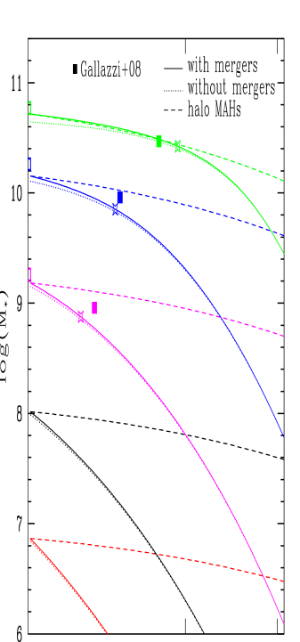
Figure 12: Average stellar mass assembly tracks inferred by means of our evolutionary parametric toy model constrained by observations (solid curves). Dotted curves show the component of these tracks due to in-situ SF. The dashed curves depict the corresponding halo MAHs renormalized in each case in order that $M_{\rm vir}$($z=0$) = $M_{*}$($z=0$). For smaller masses, the delay of the stellar mass growth with respect to the halo growth increases. Open stars correspond to the $z$ at which half of the $M_{*}$ was assembled. This characteristic $z$ estimated for SDSS galaxies by means of the archeological approach (Gallazzi et al., 2008) is shown with solid squares for three samples of galaxies, each one with an average present-day $M_{*}$ indicated by the open squares.

In Figs. 11 and 2, we plot the sSFR vs $M_{*}$ and $F_{*}$ vs $M_{\rm vir}$ isochrones obtained with this model at four epochs (blue dashed curves), respectively. The observational data related to the total sSFR -$M_{*}$ relation that we have used are taken from: Salim et al. (2007) for SDSS/GALEX galaxies at $z\approx 0$; Bell et al. (2007) for COMBO-17 galaxies at redshift bins centred at $z\sim 0.5$ and $z\sim 1$; Karim et al. (2011) for galaxies in the COSMOS field (instead of averages in mass bins, a 1.4 GHz (VLA) image stacking analysis was performed; in this case, we plot the fits to the data given in the paper); and Bauer et al. (2011) for a stellar mass-selected sample of galaxies from the GOODS NICMOS survey (their $1.5<z<2$ redshift bin is used; the data in their next bin, $2.0<z<2.5$, are actually very similar). We have converted all the samples to a Chabrier (2003) IMF. In the literature, there are many other determinations of the sSFR-$M_{*}$ relation at different epochs (see the Introduction for references) but most of them refer only to star-forming galaxies. Actually, at masses below a few $10^{10}$ $M_{*}$, the great majority of galaxies are blue/star forming, while at larger masses, the majority are red/passive galaxies. At $z>3$, even these massive galaxies can be blue/star forming. Therefore, we take care that our toy model agrees with the few available observational estimates of the sSFR-$M_{*}$ relation at high $z$ (see Fig. 4).

Regarding the empirical $F_{*}$–$M_{\rm vir}$ relations, we have used the continuous function (red triple-dot-dashed curves in Fig. 2) proposed in FA10 at $z=0-4$ for describing the abundance matching results of Behroozi, Conroy & Wechsler (2010) at two different redshift ranges: $0<z\mathchar 13358\relax 1$ and $1\mathchar 13358\relax z<4$. At the low-mass side, the decrease with $z$ of the $F_{*}$($M_{\rm vir}$,$z$) function used in FA10 is faster than the one obtained by Behroozi et al. (2010, 2012) at $0<z\mathchar 13358\relax 1$, but slower than what is reported in Yang et al. (2012).

In Fig. 12, five stellar mass growth histories obtained with this model are plotted. Solid lines depict the total (in-situ + ex-situ) mass growths, while dotted lines correspond only to the in-situ SF mode. As is seen, the ex-situ (dry merger) mode is moderately significant only for the most massive galaxy models. For present-day masses of $\mbox{$M_{*}$}\approx 5\times 10^{10}$ $M_{\odot}$, mergers contributed with the $\approx 17\%$ to the total stellar mass assembly since $z=2$. Along each track, we plot also the $z$ where half of the present-day $M_{*}$ has been attained (open stars). This characteristic redshift has been also inferred by means of stellar population synthesis models (archaeological approach) and determined for a large sample of SDSS galaxies in Gallazzi et al. (2008). Their results for three average present-day masses (open squares), close to our three most massive models, are represented in Fig. 12 with solid squares. The agreement of this quantity between our models and the archaeological inferences is encouraging. We also plot for each of our model tracks their corresponding mean halo MAHs (dashed lines) but shifted down vertically in each case in order that $\mbox{$M_{\rm vir}$}($z=0$)=\mbox{$M_{*}$}($z=0$)$. In this way, it is possible to compare the shapes of the $M_{*}$ and $M_{\rm vir}$ growth histories for each model. As the mass decreases, the delay of the active phase of stellar mass growth with respect to the halo one is more significant. The four MAHs for the lower stellar masses in Fig. 12, as well as the corresponding histories associated to $M_{*}$/$M_{\rm vir}$, were reproduced in Figs. 7, 9, and 10, in order to compare them with the results obtained in the simulations (Sec. 4.4).

References

- Aumer et al. (2013) Aumer M., White S., Naab T., Scannapieco C., 2013, ArXiv e-prints
- Avila-Reese et al. (2011) Avila-Reese V., Colín P., González-Samaniego A., Valenzuela O., Firmani C., Velázquez H., Ceverino D., 2011, ApJ, 736, 134
- Avila-Reese & Firmani (2011) Avila-Reese V., Firmani C., 2011, in RevMexAA Conference Series, Vol. 40, pp. 27–35
- Baldry, Glazebrook & Driver (2008) Baldry I. K., Glazebrook K., Driver S. P., 2008, MNRAS, 388, 945
- Bauer et al. (2011) Bauer A. E., Conselice C. J., Pérez-González P. G., Grützbauch R., Bluck A. F. L., Buitrago F., Mortlock A., 2011, MNRAS, 417, 289
- Bauer et al. (2005) Bauer A. E., Drory N., Hill G. J., Feulner G., 2005, ApJ, 621, L89
- Behroozi, Conroy & Wechsler (2010) Behroozi P. S., Conroy C., Wechsler R. H., 2010, ApJ, 717, 379
- Behroozi, Wechsler & Conroy (2013) Behroozi P. S., Wechsler R. H., Conroy C., 2013, ApJ, 770, 57
- Bell et al. (2007) Bell E. F., Zheng X. Z., Papovich C., Borch A., Wolf C., Meisenheimer K., 2007, ApJ, 663, 834
- Bouché et al. (2010) Bouché N. et al., 2010, ApJ, 718, 1001
- Bouwens et al. (2012) Bouwens R. J. et al., 2012, ApJ, 754, 83
- Brook et al. (2012) Brook C. B., Stinson G., Gibson B. K., Wadsley J., Quinn T., 2012, MNRAS, 424, 1275
- Bryan & Norman (1998) Bryan G. L., Norman M. L., 1998, ApJ, 495, 80
- Chabrier (2003) Chabrier G., 2003, PASP, 115, 763
- Christensen et al. (2012) Christensen C., Quinn T., Governato F., Stilp A., Shen S., Wadsley J., 2012, MNRAS, 425, 3058
- Colín et al. (2010) Colín P., Avila-Reese V., Vázquez-Semadeni E., Valenzuela O., Ceverino D., 2010, ApJ, 713, 535
- Conroy & Wechsler (2009) Conroy C., Wechsler R. H., 2009, ApJ, 696, 620
- Conroy, Wechsler & Kravtsov (2006) Conroy C., Wechsler R. H., Kravtsov A. V., 2006, ApJ, 647, 201
- Daddi et al. (2009) Daddi E. et al., 2009, ApJ, 694, 1517
- Damen et al. (2009) Damen M., Labbé I., Franx M., van Dokkum P. G., Taylor E. N., Gawiser E. J., 2009, ApJ, 690, 937
- Davé, Oppenheimer & Finlator (2011) Davé R., Oppenheimer B. D., Finlator K., 2011, MNRAS, 415, 11
- de Rossi, Tissera & Pedrosa (2010) de Rossi M. E., Tissera P. B., Pedrosa S. E., 2010, A&A, 519, A89+
- De Rossi, Tissera & Pedrosa (2012) De Rossi M. E., Tissera P. B., Pedrosa S. E., 2012, A&A, 546, A52
- Fakhouri, Ma & Boylan-Kolchin (2010) Fakhouri O., Ma C.-P., Boylan-Kolchin M., 2010, MNRAS, 406, 2267
- Faucher-Giguère, Kereš & Ma (2011) Faucher-Giguère C.-A., Kereš D., Ma C.-P., 2011, MNRAS, 417, 2982
- Feulner et al. (2005) Feulner G., Gabasch A., Salvato M., Drory N., Hopp U., Bender R., 2005, ApJ, 633, L9
- Firmani & Avila-Reese (2010) Firmani C., Avila-Reese V., 2010, ApJ, 723, 755
- Firmani, Avila-Reese & Rodríguez-Puebla (2010) Firmani C., Avila-Reese V., Rodríguez-Puebla A., 2010, MNRAS, 404, 1100
- Fontanot et al. (2009) Fontanot F., De Lucia G., Monaco P., Somerville R. S., Santini P., 2009, MNRAS, 397, 1776
- Gallazzi et al. (2008) Gallazzi A., Brinchmann J., Charlot S., White S. D. M., 2008, MNRAS, 383, 1439
- Gonzalez et al. (2012) Gonzalez V., Bouwens R., llingworth G., Labbe I., Oesch P., Franx M., Magee D., 2012, ArXiv e-prints
- González et al. (2011) González V., Labbé I., Bouwens R. J., Illingworth G., Franx M., Kriek M., 2011, ApJ, 735, L34
- González-Samaniego & Avila-Reese (2012) González-Samaniego A., Avila-Reese V., 2012, ”From the First Structures to the Universe Today”; eds. M.E. De Rossi, S.E. Pedrosa, L.J. Pellizza; AAA Workshop Series, in press
- Governato et al. (2010) Governato F. et al., 2010, Nature, 463, 203
- Governato et al. (2007) Governato F., Willman B., Mayer L., Brooks A., Stinson G., Valenzuela O., Wadsley J., Quinn T., 2007, MNRAS, 374, 1479
- Guo et al. (2011) Guo Q. et al., 2011, MNRAS, 413, 101
- Guo et al. (2010) Guo Q., White S., Li C., Boylan-Kolchin M., 2010, MNRAS, 404, 1111
- Hopkins, Quataert & Murray (2012) Hopkins P. F., Quataert E., Murray N., 2012, MNRAS, 421, 3522
- Huang et al. (2012) Huang S., Haynes M. P., Giovanelli R., Brinchmann J., Stierwalt S., Neff S. G., 2012, AJ, 143, 133
- Hummels & Bryan (2012) Hummels C. B., Bryan G. L., 2012, ApJ, 749, 140
- Kajisawa et al. (2010) Kajisawa M., Ichikawa T., Yamada T., Uchimoto Y. K., Yoshikawa T., Akiyama M., Onodera M., 2010, ApJ, 723, 129
- Kannan et al. (2013) Kannan R., Stinson G. S., Macciò A. V., Brook C., Weinmann S. M., Wadsley J., Couchman H. M. P., 2013, ArXiv e-prints
- Karim et al. (2011) Karim A. et al., 2011, ApJ, 730, 61
- Kauffmann et al. (2003) Kauffmann G. et al., 2003, MNRAS, 341, 33
- Kereš et al. (2009) Kereš D., Katz N., Davé R., Fardal M., Weinberg D. H., 2009, MNRAS, 396, 2332
- Khalatyan et al. (2008) Khalatyan A., Cattaneo A., Schramm M., Gottlöber S., Steinmetz M., Wisotzki L., 2008, MNRAS, 387, 13
- Kobayashi, Springel & White (2007) Kobayashi C., Springel V., White S. D. M., 2007, MNRAS, 376, 1465
- Kravtsov et al. (2004) Kravtsov A. V., Berlind A. A., Wechsler R. H., Klypin A. A., Gottlöber S., Allgood B., Primack J. R., 2004, ApJ, 609, 35
- Krumholz & Dekel (2012) Krumholz M. R., Dekel A., 2012, ApJ, 753, 16
- Kuhlen et al. (2012) Kuhlen M., Krumholz M. R., Madau P., Smith B. D., Wise J., 2012, ApJ, 749, 36
- Leauthaud et al. (2012) Leauthaud A. et al., 2012, ApJ, 744, 159
- Lee et al. (2011) Lee J. C. et al., 2011, ApJS, 192, 6
- Lee et al. (2012) Lee K.-S. et al., 2012, ApJ, 752, 66
- Leitner (2012) Leitner S. N., 2012, ApJ, 745, 149
- Liu et al. (2010) Liu L., Yang X., Mo H. J., van den Bosch F. C., Springel V., 2010, ApJ, 712, 734
- Mandelbaum et al. (2006) Mandelbaum R., Seljak U., Kauffmann G., Hirata C. M., Brinkmann J., 2006, MNRAS, 368, 715
- Marchesini et al. (2009) Marchesini D., van Dokkum P. G., Förster Schreiber N. M., Franx M., Labbé I., Wuyts S., 2009, ApJ, 701, 1765
- McCarthy et al. (2012) McCarthy I. G., Schaye J., Font A. S., Theuns T., Frenk C. S., Crain R. A., Dalla Vecchia C., 2012, MNRAS, 427, 379
- More et al. (2011) More S., van den Bosch F. C., Cacciato M., Skibba R., Mo H. J., Yang X., 2011, MNRAS, 410, 210
- Mortlock et al. (2011) Mortlock A., Conselice C. J., Bluck A. F. L., Bauer A. E., Grützbauch R., Buitrago F., Ownsworth J., 2011, MNRAS, 413, 2845
- Mosconi et al. (2001) Mosconi M. B., Tissera P. B., Lambas D. G., Cora S. A., 2001, MNRAS, 325, 34
- Moster, Naab & White (2013) Moster B. P., Naab T., White S. D. M., 2013, MNRAS, 428, 3121
- Munshi et al. (2013) Munshi F. et al., 2013, ApJ, 766, 56
- Murray, Quataert & Thompson (2005) Murray N., Quataert E., Thompson T. A., 2005, ApJ, 618, 569
- Noeske et al. (2007) Noeske K. G. et al., 2007, ApJ, 660, L47
- Oppenheimer et al. (2010) Oppenheimer B. D., Davé R., Kereš D., Fardal M., Katz N., Kollmeier J. A., Weinberg D. H., 2010, MNRAS, 406, 2325
- Papastergis et al. (2012) Papastergis E., Cattaneo A., Huang S., Giovanelli R., Haynes M. P., 2012, ApJ, 759, 138
- Piontek & Steinmetz (2011) Piontek F., Steinmetz M., 2011, MNRAS, 410, 2625
- Puchwein & Springel (2012) Puchwein E., Springel V., 2012, MNRAS, 199
- Rodríguez-Puebla, Avila-Reese & Drory (2013) Rodríguez-Puebla A., Avila-Reese V., Drory N., 2013, ApJ, 767, 92
- Rodríguez-Puebla et al. (2011) Rodríguez-Puebla A., Avila-Reese V., Firmani C., Colín P., 2011, RevMexAA, 47, 235
- Saitoh et al. (2008) Saitoh T. R., Daisaka H., Kokubo E., Makino J., Okamoto T., Tomisaka K., Wada K., Yoshida N., 2008, PASJ, 60, 667
- Salim et al. (2007) Salim S. et al., 2007, ApJS, 173, 267
- Santini et al. (2009) Santini P. et al., 2009, A&A, 504, 751
- Sawala et al. (2011) Sawala T., Guo Q., Scannapieco C., Jenkins A., White S., 2011, MNRAS, 413, 659
- Scannapieco et al. (2005) Scannapieco C., Tissera P. B., White S. D. M., Springel V., 2005, MNRAS, 364, 552
- Scannapieco et al. (2006) Scannapieco C., Tissera P. B., White S. D. M., Springel V., 2006, MNRAS, 371, 1125
- Scannapieco et al. (2008) Scannapieco C., Tissera P. B., White S. D. M., Springel V., 2008, MNRAS, 389, 1137
- Scannapieco et al. (2012) Scannapieco C. et al., 2012, MNRAS, 423, 1726
- Somerville et al. (2008) Somerville R. S. et al., 2008, ApJ, 672, 776
- Springel (2005) Springel V., 2005, MNRAS, 364, 1105
- Springel & Hernquist (2003) Springel V., Hernquist L., 2003, MNRAS, 339, 289
- Springel et al. (2001) Springel V., White S. D. M., Tormen G., Kauffmann G., 2001, MNRAS, 328, 726
- Stark et al. (2013) Stark D. P., Schenker M. A., Ellis R., Robertson B., McLure R., Dunlop J., 2013, ApJ, 763, 129
- Stewart et al. (2009) Stewart K. R., Bullock J. S., Wechsler R. H., Maller A. H., 2009, ApJ, 702, 307
- Thielemann, Nomoto & Hashimoto (1993) Thielemann F.-K., Nomoto K., Hashimoto M., 1993, in Origin and Evolution of the Elements, Prantzos N., Vangioni-Flam E., Casse M., eds., pp. 297–309
- Vale & Ostriker (2004) Vale A., Ostriker J. P., 2004, MNRAS, 353, 189
- Wake et al. (2011) Wake D. A. et al., 2011, ApJ, 728, 46
- Wang & Jing (2010) Wang L., Jing Y. P., 2010, MNRAS, 402, 1796
- Weinmann et al. (2012) Weinmann S. M., Pasquali A., Oppenheimer B. D., Finlator K., Mendel J. T., Crain R. A., Macciò A. V., 2012, MNRAS, 426, 2797
- Weinmann et al. (2006) Weinmann S. M., van den Bosch F. C., Yang X., Mo H. J., 2006, MNRAS, 366, 2
- Weisz et al. (2011) Weisz D. R. et al., 2011, ApJ, 739, 5
- Woosley & Weaver (1995) Woosley S. E., Weaver T. A., 1995, ApJS, 101, 181
- Wuyts et al. (2011) Wuyts S. et al., 2011, ApJ, 738, 106
- Yang, Mo & van den Bosch (2003) Yang X., Mo H. J., van den Bosch F. C., 2003, MNRAS, 339, 1057
- Yang et al. (2012) Yang X., Mo H. J., van den Bosch F. C., Zhang Y., Han J., 2012, ApJ, 752, 41
- Zehavi, Patiri & Zheng (2012) Zehavi I., Patiri S., Zheng Z., 2012, ApJ, 746, 145
- Zheng, Coil & Zehavi (2007) Zheng Z., Coil A. L., Zehavi I., 2007, ApJ, 667, 760