Spitzer, Gaia, and the Potential of the Milky Way

Abstract

Near-future data from ESA’s Gaia mission will provide precise, full phase-space information for hundreds of millions of stars out to heliocentric distances of $\sim$10 kpc. This “horizon” for full phase-space measurements is imposed by the Gaia parallax errors degrading to worse than 10%, and could be significantly extended by an accurate distance indicator. Recent work has demonstrated how Spitzer observations of RR Lyrae stars can be used to make distance estimates accurate to 2%, effectively extending the Gaia, precise-data horizon by a factor of ten in distance and a factor of 1000 in volume. This Letter presents one approach to exploit data of such accuracy to measure the Galactic potential using small samples of stars associated with debris from satellite destruction. The method is tested with synthetic observations of 100 stars from the end point of a simulation of satellite destruction: the shape, orientation, and depth of the potential used in the simulation are recovered to within a few percent. The success of this simple test with such a small sample in a single debris stream suggests that constraints from multiple streams could be combined to examine the Galaxy’s dark matter halo in even more detail — a truly unique opportunity that is enabled by the combination of Spitzer and Gaia with our intimate perspective on our own Galaxy.

1. Introduction

The existence of vast halos of unseen dark matter surrounding each galaxy has long been proposed to explain the surprisingly large motions of the baryonic matter that we can see (e.g., Rubin & Ford, 1970). Dark-matter-only simulations of structure formation lead us to expect that these dark matter halos should have density distributions that are described by a universal radial profile (Navarro et al., 1996) with a variety of triaxial shapes (Jing & Suto, 2002). The inclusion of baryons in the simulations tends to soften the triaxiality of the dark matter in the inner regions of the halo (e.g., as the disk forms, Bailin et al., 2005) and can alter the radial profile through a combination of adiabatic contraction and energetic feedback (e.g. Pontzen & Governato, 2012). Hence, measurements of the shape, orientation, radial profile, and extent of dark matter halos provides information about the formation of these vast structures, as well as the messy baryonic processes that continue to shape them.

The Milky Way is the best candidate for such a detailed study of a dark matter halo since we can resolve large samples of stellar tracers. Thousands of blue horizontal branch stars selected from the Sloan Digital Sky Survey (SDSS) have been used to probe the Milky Way mass out to tens of kpc (SDSS, see Deason et al., 2012a; Kafle et al., 2012), and estimates with combined tracers extend to 150kpc (Deason et al., 2012b).

This approach assumes that the tracers represent a random sampling of phase-mixed orbits drawn from a smooth distribution function, however large area surveys have revealed the existence of large-scale spatial inhomogeneities in the form of giant stellar streams (Newberg et al., 2002; Majewski et al., 2003; Belokurov et al., 2006), demonstrating that a significant fraction of the stellar halo is neither randomly sampled nor is fully phase-mixed.

A complimentary approach to measuring the mass distribution is to instead take advantage of the non-random nature of the Galaxy’s stellar distribution and utilize the knowledge that stars in streams were once all part of the same object. Such approaches can require orders of magnitude fewer tracers than a randomly sampled population to achieve comparable accuracy. One method is to simply fit orbits to observations of streams (e.g., Koposov et al., 2010). However, the assumption that debris traces a single orbit is actually incorrect (see Johnston, 1998; Helmi & White, 1999) and changes in orbital properties along debris streams can lead to systematic biases in measurements of the Galactic potential (Eyre & Binney, 2009; Varghese et al., 2011). Sanders & Binney (2013a) recently demonstrated that this bias is equally problematic for the very thinnest, coldest streams, whose observed properties may be indistinguishable from those of the parent orbit (e.g. such as the globular cluster, GD1 — see Koposov et al., 2010), as for the much more extended and hotter streams (e.g. such as debris from the Sagittarius dwarf galaxy — see Majewski et al., 2003) where offsets from a single orbit are clearly apparent.

One way to address these biases is to run self-consistent N-body simulations of satellite destruction in a variety of potentials with the aim of simultaneously constraining both the properties of the satellite and the Milky Way. Many studies of the Sagittarius debris system (hereafter Sgr) have adopted this approach, with the most recent work attempting to place constraints on the triaxiality and orientation of the dark matter halo (Law & Majewski, 2010).

The promise of near-future data sets including full phase-space information has also inspired other approaches. Binney (2008) and Peñarrubia et al. (2012) demonstrate that the distribution of energy and entropy in debris, respectively, will be minimized only for a correct assumption of the form of the Galactic potential. Sanders & Binney (2013b) examine the distribution of debris in action-angle co-ordinates and show that stars stripped from the same disrupted object must lie along a single line in angle-frequency space, providing a constraint that can be used as a potential measure.

In this Letter we re-examine and update a complimentary approach to using tidal debris as a potential measure (originally proposed by Johnston et al., 1999b) in the context of current and near-future observational capabilities, and apply it to a simulation of the Sgr debris system. In Section 2 we outline the observational prospects and Sgr properties that motivated this re-examination. In Section 3 we present the updated potential measure and test it with synthetic observations of simulated Sgr debris. In Section 4 we highlight the advantages and shortcomings of this method. We conclude in Section 5.

2. Context and motivation

The method presented in Section 3 takes advantage of three distinct developments: (i) the demonstration of a technique for deriving distances to individual RR Lyrae stars with 2% accuracies (Section 2.1); (ii) the prospect of proper motion measurements of the same stars with $\sim$10 $\mu$as/yr precision (Section 2.2); and (iii) the tracing of debris associated with Sgr around the entire Galaxy (Section 2.3)

2.1. Spitzer and 2% distance errors to RR Lyrae in the halo

There is a long tradition for using RR Lyrae stars in the Galaxy to study structure (e.g. Shapley, 1918), substructure (e.g. Sesar et al., 2010), and distances to satellite galaxies (e.g. Clementini et al., 2003). However, studies of RR Lyrae at optical wavelengths are limited by both metallicity effects on the intrinsic brightness of these stars and variable extinction along the line of sight. Moreover, systematic differences between instruments make it difficult to tie observations across the sky to a common scale.

At longer wavelengths, RR Lyrae promise tighter constraints on distances. Madore & Freedman (2012) have recently shown, using five stars with trigonometric parallaxes measured by Hubble (Benedict et al., 2011), that the dispersion in the mid-IR Period-Luminosity (PL) relation (first mapped by Longmore et al., 1986) at wavelengths measurable by NASA’s Spitzer mission is $\sim$0.03 mag. This implies that it is possible to use Spitzer to determine distances that are good to $2\%$ for individual RR Lyrae stars out to $\sim$60 kpc (Spitzer’s limit for detecting and measuring RR Lyrae). For comparison, distance measurements of Blue Horizontal Branch stars typically achieve $\sim$10-15% uncertainties (if appropriate color measurements are available, e.g., Deason et al., 2012b).

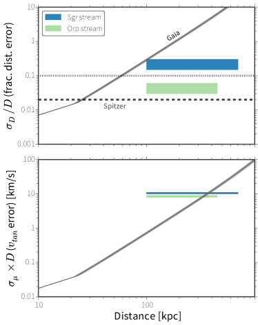
Figure 1.— Expected Gaia distance and tangential velocity errors as a function of heliocentric distance for RR Lyrae stars. Errors are a function of color and magnitude of the source, and hence the metallicity: each line is computed by Monte Carlo sampling from the empirical metallicity distribution of the Galactic halo from Ivezić et al. (2008). Parallax distance errors from Gaia are larger than the line-of-sight size of both Sgr and Orphan (Orp), but photometric distance errors are comparable to the the Sgr scale (assuming 10% errors, dotted line). Bottom panel shows that the Gaia tangential velocity errors are smaller than the internal velocity dispersion of nearer regions of both Sgr and Orp.

2.2. Gaia and the age of astrometry

The Gaia satellite (Perryman et al., 2001) is an astrometric mission which aims to measure the positions of billions of stars with 10-100 $\mu$as accuracies. Combined with expected proper motion accuracies, this will enable full six-dimensional phase-space maps of the Galaxy with $<$10% distance errors for heliocentric distances of up to $\sim$6 kpc for RR Lyrae stars.

Figure 1 shows the Gaia end-of-mission distance and tangential velocity error estimates for RR Lyrae. Within 2 kpc, Gaia will measure distances to these stars with better than 2% accuracy — RR Lyrae in this volume can be used to test and calibrate the Spitzer PL relation described above. Beyond the 2 kpc threshold, the mid-IR PL relation for RR Lyrae will provide better distance measurements.

The combination of Spitzer and Gaia data will extend the “horizon” of where precise, six-dimensional phase-space maps of the Galaxy are possible from $<$10 kpc to 60 kpc. This enormous increase in volume will greatly refine data on debris systems in the halo.

2.3. The Sagittarius debris system

Sgr was discovered serendipitously during a radial velocity survey of the Galactic bulge (Ibata et al., 1994). Signatures of extensive stellar streams associated with Sgr have since been mapped across the sky in carbon stars (Totten & Irwin, 1998), M giants selected from 2MASS (Majewski et al., 2003), main sequence turnoff stars from SDSS (Belokurov et al., 2006), and RR Lyrae in the Catalina Sky Survey (Drake et al., 2013).

Sgr stream data has inspired a rich set of models (e.g., Johnston et al., 1999a; Fellhauer et al., 2006). Most recently, Law & Majewski (2010, hereafter LM10) combined all the (then) current data on the Sgr debris to constrain both a model of its evolution and the potential in which it orbits. (Note that new observational work by Belokurov et al. (2013) suggest that the trailing tail of Sgr debris does not match the LM10 model.) Figure 2 shows particle positions from the final time-step of the LM10 N-body simulation of dwarf satellite disruption along the expected Sgr orbit in the best-fitting Milky Way halo model. The simulation was run in a three-component potential, with a triaxial, logarithmic halo model of the form

$$\Phi_{halo}=v_{halo}^{2}\ln(C_{1}x^{2}+C_{2}y^{2}+C_{3}xy+(z/q_{z})^{2}+R_{c}^{2})$$ (1)

where $C_{1}$, $C_{2}$, and $C_{3}$ are combinations of the $x$ and $y$ axis ratios ($q_{1}$, $q_{2}$) and orientation of the halo with respect to the baryonic disk ($\phi$):

$$C_{1} =\frac{\cos^{2}\phi}{q_{1}^{2}}+\frac{\sin^{2}\phi}{q_{2}^{2}}$$ (2)

$$C_{2} =\frac{\sin^{2}\phi}{q_{1}^{2}}+\frac{\cos^{2}\phi}{q_{2}^{2}}$$ (3)

$$C_{3} =2\sin\phi\cos\phi\left(q_{1}^{-2}-q_{2}^{-2}\right).$$ (4)

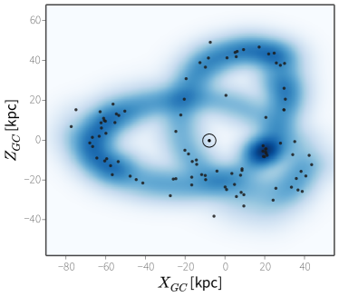
Figure 2.— Particle density (blue) of the first leading and trailing wraps from the final time-step of the Law & Majewski (2010) simulation of the Sgr stream. Point markers (black) show positions of a random sample of 100 stars drawn from this density distribution. The position of the Sun is shown with the solar symbol.

A comparison of simulations and data enabled LM10 to make an assessment of the three-dimensional mass distribution of the Milky Way’s dark matter halo through constraints on the potential parameters $v_{\rm halo}$, $q_{1}$, $q_{z}$, and $\phi$. Combined Spitzer and Gaia measurements of distances and proper motions of RR Lyrae in the Sgr debris will open up new avenues for potential constraints. Figure 1 shows that a 2% distance error is smaller than the distance range in the stream (top panel). Similarly, Gaia proper motion error estimates correspond to tangential velocity errors less than the velocity dispersion for much of the stream (bottom panel). The next section outlines a new method to take advantage of this information.

3. Description and test of our algorithm

With access to 6D information for stars in a tidal stream, each star becomes a powerful potential measure by exploiting the fact that the stars must have come from the same progenitor: if the orbits of the stars and progenitor are integrated backwards in a a potential that accurately models the Milky Way, the stars should recombine with the progenitor (imagine watching satellite destruction in “rewind”). If the potential is incorrect, the orbits of the stars will diverge from that of the progenitor and thus will not be recaptured by the satellite system (Figure 3).

This approach was originally proposed by Johnston et al. (1999b) and was tested on the proposed characteristics of the Space Interferometry Mission (Unwin et al., 2008). Below we present an updated version of the algorithm: the promise of 2% distances to RR Lyrae stars (see Section 2.1) enables a direct measurement (rather than approximate estimate, as previously assumed) of the position of a star within its debris structure. The test statistic that quantifies how well stars recombine with the satellite has also been rigorously redefined.

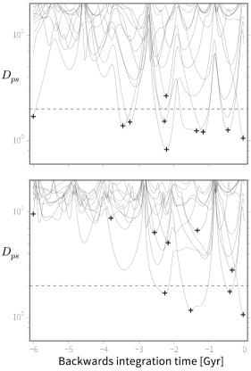
Figure 3.— Phase space distance ($D_{\rm ps}$) for 10 randomly selected stars integrated backwards in the correct potential (top) and a potential where $q_{z}$ is 25% larger (bottom). The same 10 particles are used in both figures, so the initial conditions are identical. Horizontal (dashed) line shows $D_{\rm ps}=2$, for reference.

3.1. The algorithm: Rewinder

Quantifying this method requires a sample of stars with known full space kinematics $(\boldsymbol{x}_{i},\boldsymbol{v}_{i})|_{t=0}$ (e.g., measurements of all position and velocity components for these stars today at $t=0$), the orbital parameters for the progenitor system $(\boldsymbol{x}_{p},\boldsymbol{v}_{p})|_{t=0}$, and a functional form for the potential, $\Phi({\boldsymbol{\theta}})$. For a given set of potential parameters, $\boldsymbol{\theta}$, the orbits of the stars and progenitor are integrated backwards for several Gigayears. At each timestep $t_{j}$, for each particle $i$, a set of normalized, relative phase-space coordinates are computed

$$\boldsymbol{q}_{i}=\frac{\boldsymbol{x}_{i}-\boldsymbol{x}_{p}}{R_{\rm tide}}\,\,\,\,,\,\,\,\,\boldsymbol{p}_{i}=\frac{\boldsymbol{v}_{i}-\boldsymbol{v}_{p}}{v_{\rm esc}}$$ (5)

where $(\boldsymbol{x},\boldsymbol{v})_{i}$ and $(\boldsymbol{x},\boldsymbol{v})_{p}$ are the phase-space coordinates for the particles and progenitor, respectively. These definitions require an estimate of the mass of the satellite, $m_{sat}$, which, combined with the orbital radius of the satellite, $R$, and the computed enclosed mass of the potential within $R$, $M_{enc}$, sets the instantaneous tidal radius and escape velocity,

$$R_{\rm tide}=R\Big{(}\frac{m_{\rm sat}}{3M_{\rm enc}}\Big{)}^{1/3}\,\,\,\,,\,\,\,\,v_{\rm esc}=\sqrt{\frac{2Gm_{\rm sat}}{R_{\rm tide}}}.$$ (6)

These quantities are computed at each time step to take the time dependence into account, neglecting mass-loss from the satellite. Qualitatively, when the distance in this normalized six-dimensional space, $D_{{\rm ps},i}=\sqrt{|\boldsymbol{q}_{i}|^{2}+|\boldsymbol{p}_{i}|^{2}}\lesssim 2$, the star is likely recaptured by the satellite (in the absence of errors, we find that $\sim$90% of the initially bound particles come within this limit when integrating all orbits backwards). Johnston et al. (1999b) imposed a similar condition as a hard boundary and maximized the number of recaptured particles in a given backwards-integration. What follows is a description of an updated procedure with a statistically-motivated choice for an objective function.

For each star, $i$, the phase-space distance, $D_{\rm ps}$, is computed at each timestep $t_{j}$, and the vector with the minimum phase-space distance is stored

$$t^{*}_{i} =\operatornamewithlimits{argmin}_{t}D_{{\rm ps},i}$$ (7)

$$\boldsymbol{A}_{i} =(\boldsymbol{q}_{i}(t^{*}_{i}),\boldsymbol{p}_{i}(t^{*}_{i})).$$ (8)

Thus, the matrix $\boldsymbol{A}_{ik}$ contains these minimum phase-space distance vectors for each star, where $k\in[1,6]$. Intuitively, the variance of the distribution of minimum phase-space vectors will be larger for orbits integrated in an incorrect potential relative to the distribution computed from the ‘true’ orbital history of the stars: in an incorrect potential, the orbits of the stars relative to the orbit of the progenitor spread out in phase space. Thus, the generalized variance of the distribution — computed for a given set of potential parameters, $\boldsymbol{\theta}$ — is a natural choice for the scalar objective function, $f(\boldsymbol{\theta})$, used in constraining the potential of the Milky Way

$$\Sigma_{n} =\mathrm{Cov}(\boldsymbol{A}_{ik})$$ (9)

$$f(\boldsymbol{\theta}) =\ln\det\Sigma_{n}.$$ (10)

3.2. Application to Simulated Data

The LM10 simulation data (see Section 2.3) is a perfect test-bed for evaluating the effectiveness of this method. We start by extracting both particle data and the satellite orbital parameters from the present-day snapshot of the simulation data. We then “observe” a sample of 100 stars from the first leading and trailing wraps of the stream. The radial velocity and distance errors are drawn from Gaussians ($\varepsilon_{\rm RV}\sim\mathcal{N}(\mu=0,\sigma=10~{}{\rm km/s})$ and $\varepsilon_{\rm D}\sim\mathcal{N}(0,0.02\times D)$) and the proper motion errors are computed from the expected Gaia error curve.

The generalized variance defines a convex function over which we optimize four of the six logarithmic potential parameters: $v_{circ}$, $\phi$, $q_{1}$, and $q_{z}$ ($q_{2}$ and $R_{c}$ are degenerate with combinations of the other parameters). Figure 4 shows one-dimensional slices of the objective function produced by varying each of the potential parameters by $\pm 10\%$ around the true values and holding all others fixed.

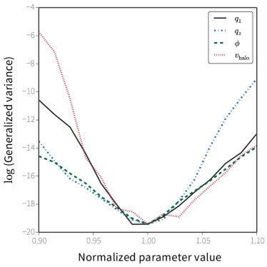
Figure 4.— 1D slices of the objective function (generalized variance) for each halo potential parameter. The parameter values are normalized by the true values show the effect of varying each parameter by $\pm 10$%. The values of the objective function (vertical axis) are not interesting but note the minima around the truth (1.0).

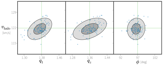
Figure 5.— Blue points show the “best-fit” parameters resulting from each resample of 100 stars from the Sgr stream particle density shown in Figure 2. Green (vertical and horizontal) lines show the true values of the parameters. Grey ellipses show one- and two-sigma margins, assuming the points are normally distributed.

In anticipation of extending the above method to include a true likelihood function, we use a parallelized Markov Chain Monte Carlo (MCMC) algorithm (Foreman-Mackey et al., 2013) to sample from our objective function. We use the median value of the converged sample distribution as a point estimate for the potential parameters. To assess the uncertainty in the derived halo parameters, we sample 100 stars 100 times and estimate the potential parameters with each resampling. Figure 5 shows the recovered parameters for each sample and demonstrates the power of this method: a moderately sized sample of RR Lyrae alone places strong constraints on the shape and mass of the Galaxy’s dark matter halo. From the covariance matrix derived from the distribution of points in Figure 5, we find the mean recovered parameters and one-sigma deviations to be $q_{1}=1.36\pm 0.02$, $q_{z}=1.36\pm 0.03$, $\phi=96.0\pm 1.5$ degrees, and $v_{\rm halo}=123.2\pm 1.6$ km/s.

4. Discussion, strengths, and limitations

The strengths of this method stem from its simplicity: it requires only a rough estimate of the satellite mass $m_{\rm sat}$ combined with backwards integration of orbits. Rewinder does not assume that stream stars follow a single orbit and instead relies on the fact that each star is on a different orbit. There are also no assumptions made about of the internal distribution of satellite stars. Thus, Rewinder is applicable to any debris that is known to come from a single object and not restricted to the coldest tidal streams. In principle, it could also be applied to the vast stellar debris clouds that have been discovered (e.g., the Triangulum-Andromeda and Hercules-Aquila clouds; Rocha-Pinto et al., 2004; Belokurov et al., 2006), or even stars that have only associations in orbital properties and do not form a coherent spatial structure (e.g. Helmi & White, 1999). The method trivially extends to combining constraints from multiple debris systems at once by simply integrating all debris from several satellites simultaneously, with $D_{\rm ps}$ defined appropriately for each star.

It is also important to characterize the the limitations of this method. Firstly, the measurement errors for RR Lyraes associated with the very coldest streams (e.g., the globular clusters Pal5 and GD1; Odenkirchen et al., 2002; Koposov et al., 2010) will likely be too large to resolve the minute differences in orbital properties between the debris and satellite. Second, the present prescription neglects orbital evolution (e.g., dynamical friction) and scattering of stream stars due to the potential of the satellite. Preliminary simulations (to be fully explored in forthcoming work) suggest that these two points can be neglected for satellite masses between $\sim$$10^{7}$ and $\sim$$10^{9}~{}\mathrm{M}_{\odot}$. Lastly, the current version of the algorithm relies on knowledge of the current position and velocity of the parent satellite, which may not be available (e.g., the Orphan Stream; Belokurov et al., 2007).

5. Conclusions and motivation for future work

This paper presents an algorithm for measuring the Galactic potential that anticipates combined data from the Spitzer and Gaia satellite missions which promise precise, full phase-space measurements of RR Lyrae stars in the halo of our Galaxy. When applied to a sample of 100 stars (with realistic observational errors) drawn from the Law & Majewski (2010) N-body simulation of the destruction of the Sgr dwarf satellite, Rewinder recovers the depth, shape, and orientation of the dark matter potential to within a few percent.

While the tests presented in this paper are very simple, the accuracy of potential recovery promised by such a small sample of stars provides strong motivation for further theoretical work to: 1) develop a robust generative model that utilizes the concepts demonstrated by Rewinder; 2) investigate the power of using multiple debris structures; and 3) examine how Rewinder might work with less accurate measurements or missing dimensions.

Our results also motivate an observational campaign with Spitzer to survey RR Lyrae stars in debris structures around the Milky Way to get precise distances to combine with near-future Gaia velocity data. If just 100 stars in a single stellar stream allow us to study the depth, shape, and orientation of the Milky Way potential, larger samples in multiple structures (e.g., the Orphan Stream; Sesar et al., 2013) offer the prospect of assessing these quantities as a function of Galactocentric radius. Tracing the mass in a dark matter halo with this level of detail is impossible for any other galaxy in the Universe.

References

- Bailin et al. (2005) Bailin, J., Kawata, D., Gibson, B. K., et al. 2005, ApJ, 627, L17
- Belokurov et al. (2006) Belokurov, V., Zucker, D. B., Evans, N. W., et al. 2006, ApJ, 642, L137
- Belokurov et al. (2007) Belokurov, V., Evans, N. W., Irwin, M. J., et al. 2007, ApJ, 658, 337
- Belokurov et al. (2013) Belokurov, V., Koposov, S. E., Evans, N. W., et al. 2013, ArXiv e-prints
- Benedict et al. (2011) Benedict, G. F., McArthur, B. E., Feast, M. W., et al. 2011, AJ, 142, 187
- Binney (2008) Binney, J. 2008, MNRAS, 386, L47
- Clementini et al. (2003) Clementini, G., Gratton, R., Bragaglia, A., et al. 2003, AJ, 125, 1309
- Deason et al. (2012a) Deason, A. J., Belokurov, V., Evans, N. W., & An, J. 2012a, MNRAS, 424, L44
- Deason et al. (2012b) Deason, A. J., Belokurov, V., Evans, N. W., et al. 2012b, MNRAS, 425, 2840
- Drake et al. (2013) Drake, A. J., Catelan, M., Djorgovski, S. G., et al. 2013, ApJ, 763, 32
- Eyre & Binney (2009) Eyre, A., & Binney, J. 2009, MNRAS, 400, 548
- Fellhauer et al. (2006) Fellhauer, M., Belokurov, V., Evans, N. W., et al. 2006, ApJ, 651, 167
- Foreman-Mackey et al. (2013) Foreman-Mackey, D., Hogg, D. W., Lang, D., & Goodman, J. 2013, PASP, 125, 306
- Helmi & White (1999) Helmi, A., & White, S. D. M. 1999, MNRAS, 307, 495
- Ibata et al. (1994) Ibata, R. A., Gilmore, G., & Irwin, M. J. 1994, Nature, 370, 194
- Ivezić et al. (2008) Ivezić, Ž., Sesar, B., Jurić, M., et al. 2008, ApJ, 684, 287
- Jing & Suto (2002) Jing, Y. P., & Suto, Y. 2002, ApJ, 574, 538
- Johnston (1998) Johnston, K. V. 1998, ApJ, 495, 297
- Johnston et al. (1999a) Johnston, K. V., Majewski, S. R., Siegel, M. H., Reid, I. N., & Kunkel, W. E. 1999a, AJ, 118, 1719
- Johnston et al. (1999b) Johnston, K. V., Zhao, H., Spergel, D. N., & Hernquist, L. 1999b, ApJ, 512, L109
- Kafle et al. (2012) Kafle, P. R., Sharma, S., Lewis, G. F., & Bland-Hawthorn, J. 2012, ApJ, 761, 98
- Koposov et al. (2010) Koposov, S. E., Rix, H.-W., & Hogg, D. W. 2010, ApJ, 712, 260
- Law & Majewski (2010) Law, D. R., & Majewski, S. R. 2010, ApJ, 714, 229
- Longmore et al. (1986) Longmore, A. J., Fernley, J. A., & Jameson, R. F. 1986, MNRAS, 220, 279
- Madore & Freedman (2012) Madore, B. F., & Freedman, W. L. 2012, ApJ, 744, 132
- Majewski et al. (2003) Majewski, S. R., Skrutskie, M. F., Weinberg, M. D., & Ostheimer, J. C. 2003, ApJ, 599, 1082
- Navarro et al. (1996) Navarro, J. F., Frenk, C. S., & White, S. D. M. 1996, ApJ, 462, 563
- Newberg et al. (2002) Newberg, H. J., Yanny, B., Rockosi, C., et al. 2002, ApJ, 569, 245
- Odenkirchen et al. (2002) Odenkirchen, M., Grebel, E. K., Dehnen, W., Rix, H.-W., & Cudworth, K. M. 2002, AJ, 124, 1497
- Peñarrubia et al. (2012) Peñarrubia, J., Koposov, S. E., & Walker, M. G. 2012, ApJ, 760, 2
- Perryman et al. (2001) Perryman, M. A. C., de Boer, K. S., Gilmore, G., et al. 2001, A&A, 369, 339
- Pontzen & Governato (2012) Pontzen, A., & Governato, F. 2012, MNRAS, 421, 3464
- Rocha-Pinto et al. (2004) Rocha-Pinto, H. J., Majewski, S. R., Skrutskie, M. F., Crane, J. D., & Patterson, R. J. 2004, ApJ, 615, 732
- Rubin & Ford (1970) Rubin, V. C., & Ford, Jr., W. K. 1970, ApJ, 159, 379
- Sanders & Binney (2013a) Sanders, J. L., & Binney, J. 2013a, MNRAS, 433, 1813
- Sanders & Binney (2013b) —. 2013b, MNRAS, 433, 1826
- Sesar et al. (2010) Sesar, B., Ivezić, Ž., Grammer, S. H., et al. 2010, ApJ, 708, 717
- Sesar et al. (2013) Sesar, B., Grillmair, C. J., Cohen, J. G., et al. 2013, ApJ, 776, 26
- Shapley (1918) Shapley, H. 1918, ApJ, 48, 154
- Totten & Irwin (1998) Totten, E. J., & Irwin, M. J. 1998, MNRAS, 294, 1
- Unwin et al. (2008) Unwin, S. C., Shao, M., Tanner, A. M., et al. 2008, PASP, 120, 38
- Varghese et al. (2011) Varghese, A., Ibata, R., & Lewis, G. F. 2011, MNRAS, 417, 198