Sparse Command Generator for Remote Control

Abstract.

In this article, we consider remote-controlled systems, where the command generator and the controlled object are connected with a bandwidth-limited communication link. In the remote-controlled systems, efficient representation of control commands is one of the crucial issues because of the bandwidth limitations of the link. We propose a new representation method for control commands based on compressed sensing. In the proposed method, compressed sensing reduces the number of bits in each control signal by representing it as a sparse vector. The compressed sensing problem is solved by an $\ell^{1}\text{-}\ell^{2}$ optimization, which can be effectively implemented with an iterative shrinkage algorithm. A design example also shows the effectiveness of the proposed method.

1. Introduction

Compressed sensing has recently been a focus of intensive researches in the signal processing community. It aims at reconstructing a signal by assuming that the original signal is sparse [2]. The core idea used in this area is to introduce a sparsity index in the optimization. The sparsity index of a vector ${\boldsymbol{v}}$ is defined by the amount of nonzero elements in ${\boldsymbol{v}}$ and is usually denoted by $\|{\boldsymbol{v}}\|_{0}$, called the “$\ell^{0}$ norm.” The compressed sensing decoding problem is then formulated by least squares with $\ell^{0}$-norm regularization. The associated optimization problem is however hard to solve, since it is a combinatorial one. Thus, it is common to introduce a convex relaxation by replacing the $\ell^{0}$ norm with the $\ell^{1}$ norm [3]. Under some assumptions, the solution of this relaxed optimization is known to be exactly the same as that of the $\ell^{0}$-norm regularization [8, 2]. That is, by minimizing the $\ell^{1}$-regularized least squares, or by $\ell^{1}\text{-}\ell^{2}$ optimization, one can obtain a sparse solution. Moreover, recent studies have examined fast algorithms for $\ell^{1}\text{-}\ell^{2}$ optimization [5, 1, 15].

The purpose of this paper is to investigate the use of sparsity-inducing techniques for remote control [11], see [10] for an alternative approach. In remote-controlled systems, control information is transmitted through bandwidth-limited channels such as wireless channels [14] or the Internet [9]. There are two approaches to reduce the number of bits transmitted on a wireless link, source coding and channel coding approaches [4]. In the former, information compression techniques reduce the number of bits to be transmitted. In the latter, efficient forward error-correcting codes reduce redundant data (i.e., parity) in channel-coded information. In this paper, we study the former approach and propose a sparsity-inducing technique to produce sparse representation of control commands, which can reduce the number of bits in transmitted data.

Our optimization to obtain sparse representation of control commands is formulated as follows: we measure the tracking error in the output trajectory of a controlled system by its $\ell^{2}$ norm, and add an $\ell^{1}$ penalty to achieve sparsity of transmitted vector. This is an $\ell^{1}$-regularized $\ell^{2}$-optimization, or shortly $\ell^{1}\text{-}\ell^{2}$-optimization, which is effectively solved by the iterative shrinkage method mentioned above. The problem of command generator has been solved when the penalty is taken solely as an $\ell^{2}$ norm, the solution of which is given by a linear combination of base functions, called control theoretic splines [13]. In this work, we also present a simple method for achieving sparse control vectors when the control commands are assumed to be in a subspace of these splines. An example illustrates the effectiveness of our method compared with the $\ell^{2}$ optimization.

Notation

For a vector ${\boldsymbol{v}}=[v_{1},\ldots,v_{n}]^{\top}\in{\mathbb{R}}^{n}$, the $\ell^{1}$ and $\ell^{2}$ norms are respectively defined by $\|{\boldsymbol{v}}\|_{1}:=\sum_{i=1}^{n}|v_{i}|$ and $\|{\boldsymbol{v}}\|_{2}:=\sqrt{{\boldsymbol{v}}^{\top}{\boldsymbol{v}}}$. For a real number $x\in{\mathbb{R}}$,

$$\mathrm{sgn}(x):=\begin{cases}1,\quad\text{if}~{}~{}x\geq 0,\\ -1,\quad\text{if}~{}~{}x<0,\end{cases},~{}(x)_{+}:=\max\{x,0\}.$$

We denote the determinant of a square matrix $M$ by $\det(M)$, and the maximum eigenvalue of a symmetric matrix $M$ by $\lambda_{\max}(M)$. Let $L^{2}[0,T]$ be the set of Lebesgue square integrable functions on $[0,T]$. For $f,g\in L^{2}[0,T]$, the inner product is defined by

$$\langle f,g\rangle:=\int_{0}^{T}f(t)g(t){\mathrm{d}}t.$$

2. Command Generation Problem

Let us consider the following linear SISO (Single-Input Single-Output) plant:

(1) $$P:\left\{\begin{split}\dot{{\boldsymbol{x}}}(t)&=A{\boldsymbol{x}}(t)+{\boldsymbol{b}}u(t),&\\ y(t)&={\boldsymbol{c}}^{\top}{\boldsymbol{x}}(t),\quad t\in[0,\infty),\quad x(0)=0,\end{split}\right.$$

where $A\in{\mathbb{R}}^{n\times n}$, ${\boldsymbol{b}}\in{\mathbb{R}}^{n}$ and ${\boldsymbol{c}}\in{\mathbb{R}}^{n}$. We assume that the system $P$ is stable and the state space realization (1) is reachable and observable. The output reference signal is given by data points $\mathcal{D}:=\{(t_{1},Y_{1}),(t_{2},Y_{1}),\ldots(t_{N},Y_{N})\}$, where $t_{i}$’s are time instants such that $0<t_{1}<t_{2}<\cdots<t_{N}=:T$. Our objective here is to design the control signal $u(t)$ such that the output trajectory $y(t)$ is close to the data points $Y_{1}$,…,$Y_{N}$ at $t=t_{1},\ldots,t_{N}$, that is, $y(t_{i})\approx Y_{i}$, $i=1,\ldots,N$. To measure the difference between $\{y(t_{i})\}_{i=1}^{N}$ and $\{Y_{i}\}_{i=1}^{N}$, we adopt the square-error cost function

$${\bf{E}}_{2}(u)=\sum_{i=1}^{N}(y(t_{i})-Y_{i})^{2},$$

where we have made the dependence of $y(t_{i})$ on $u=\{u(t)\}_{t\in[0,T]}$ through the system equation (1).

In principle, one can achieve perfect tracking, that is, ${\bf{E}}_{2}=0$, by some input signal. However, the optimal input for perfect tracking has very large gain especially when the number $N$ is very large, and may lead to oscillation between the sampling instants $t_{1},\ldots,t_{N}$. This phenomenon is known as overfitting [12]. To avoid this, one can adopt a regularization or smoothing technique. This method is to add a regularization term ${\bf{\Omega}}(u)$ to the cost function ${\bf{E}}_{2}(u)$. We formulate our problem as follows:

Problem 1.

Given data $\mathcal{D}$, find a control signal $u$ which minimizes the regularized cost function ${\bf{J}}(u)={\bf{E}}_{2}(u)+\mu{\bf{\Omega}}(u)$, where $\mu>0$ is the regularization parameter which specifies the tradeoff between minimization ${\bf{E}}_{2}(u)$ and the smoothness by ${\bf{\Omega}}(u)$.

A well-known regularization is to use $L^{2}$ function for ${\bf{\Omega}}(u)$, called the control theoretic smoothing spline [13, 6]. We review this in the next section.

3. $\ell^{2}$ Command Design by Control Theoretic Smoothing Splines

For the problem given in section 2, the following $L^{2}$-regularized cost function was considered in [13]:

(2) $${\bf{J}}_{2}(u):={\bf{E}}_{2}(u)+\mu{\bf{\Omega}}_{2}(u),\quad{\bf{\Omega}}_{2}(u):=\int_{0}^{T}u(t)^{2}{\mathrm{d}}t.$$

The optimal control $u^{\ast}_{2}$ which minimizes ${\bf{J}}_{2}(u)$ is given by a linear combination of the following functions called control theoretic splines [13, 6]:

Figure 1. Control theoretic spline $g_{i}(t)$ (solid) and the impulse response $P(t)$ of the plant $P$ (dots).

(3) $$g_{i}(t):=\begin{cases}{\boldsymbol{c}}^{\top}{\mathrm{e}}^{A(t_{i}-t)}{\boldsymbol{b}},&\quad\text{if}~{}~{}t_{i}>t,\\ 0,&\quad\text{if}~{}~{}t_{i}\leq t,\end{cases}$$

see Fig. 1. More precisely, the optimal control for (2) is given by

(4) $$u_{2}^{\ast}(t) =\sum_{i=1}^{N}\theta_{i}g_{i}(t)={\boldsymbol{g}}(t)^{\top}{\boldsymbol{\theta}}_{2}^{\ast},$$

(5) $${\boldsymbol{\theta}}_{2}^{\ast} :=(\mu I+G)^{-1}{\boldsymbol{y}}_{\text{ref}},$$

where ${\boldsymbol{g}}(t):=[g_{1}(t),\ldots,g_{N}(t)]^{\top}$, ${\boldsymbol{y}}_{\text{ref}}:=[Y_{1},\ldots,Y_{N}]^{\top}$, and $G$ is the Grammian matrix of $\{g_{1},\ldots,g_{N}\}$, defined by $[G]_{ij}:=\langle g_{i},g_{j}\rangle$, $i,j=1,\ldots,N$.

Figure 2. Remote-controlled system optimized with ${\bf{J}}_{2}(u)$ in (2). The vector ${\boldsymbol{\theta}}_{2}^{\ast}$ is transmitted through a communication channel.

4. $\ell^{1}\text{-}\ell^{2}$ Command Design for Sparse Remote Control

In remote-controlled systems, we transmit the control input $u=\{u(t)\}_{t\in[0,T]}$ to the system $P$ through a communication channel. Since $\{u(t)\}_{t\in[0,T]}$ is a continuous-time signal, we should discretize it.

An easy way to communicate information on the input signal is to transmit the data ${\boldsymbol{y}}_{\text{ref}}$ itself, and produce the input $u(t)$ by the formulae (4) and (5) at the receiver side. The vector ${\boldsymbol{y}}_{\text{ref}}$ is just an $N$-dimensional one, and much easier to transmit than the infinite-dimensional vector $\{u(t)\}_{t\in[0,T]}$.

An alternative method consists in transmitting the coefficient vector ${\boldsymbol{\theta}}_{2}^{\ast}$ given in (5) instead of the continuous-time signal $u$. This procedure is shown in Fig. 2. In this procedure, we fix the sampling instants $t_{1},\ldots,t_{N}$ and the vector ${\boldsymbol{y}}_{\text{ref}}$ is given. We first compute the parameter vector ${\boldsymbol{\theta}}_{2}^{\ast}$ by (5), and transmit this through a communication channel. The transmitted vector is received at the receiver, and then the control signal $u^{\ast}_{2}(t)$ is computed by (4), and applied to the plant $P$. We assume that the time instants $t_{1},\ldots,t_{N}$ are shared at the transmitter and the receiver.

A problem of the above-mentioned strategies is that the communication channel is band-limited and therefore the vector to be transmitted has to be first quantized and encoded. To solve this, we will seek a sparse representation of the transmitted vector ${\boldsymbol{\theta}}$ in accordance with the notion of compressed sensing [2, 7].

Define a subspace $\mathcal{V}$ of $L^{2}[0,T]$ by

(6) $$\mathcal{V}:=\left\{u\in L^{2}[0,T]:u=\sum_{j=1}^{M}\theta_{j}\phi_{j},~{}\theta_{i}\in{\mathbb{R}}\right\},$$

where $\phi_{1},\ldots,\phi_{M}$ are linearly independent vectors in $L^{2}[0,T]$. Note that if $M=N$ and $\phi_{i}=g_{i}$, $i=1,\ldots,N$ defined in (3), the optimal control $u^{\ast}_{2}(t)$ in (4) belongs to this subspace. We assume that the control $u$ is in $\mathcal{V}$, that is, we find a control $u$ in this subset. Under this assumption, the squared-error cost function ${\bf{E}}_{2}(u)$ is represented by

(7) $${\bf{E}}_{2}(u)=\sum_{i=1}^{N}(y(t_{i})-Y_{i})^{2}=\left\|\Phi{\boldsymbol{\theta}}-{\boldsymbol{y}}_{\text{ref}}\right\|_{2}^{2},$$

where $[\Phi]_{ij}=\langle g_{i},\phi_{j}\rangle$, $i=1,\ldots,N$, $j=1,\ldots,M$. To induce sparsity in ${\boldsymbol{\theta}}$, we adopt $\ell^{1}$ penalty on ${\boldsymbol{\theta}}$ and introduce the following mixed $\ell^{1}\text{-}\ell^{2}$ cost function:

(8) $${\bf{J}}_{1}({\boldsymbol{\theta}}):=\frac{1}{2}\left\|\Phi{\boldsymbol{\theta}}-{\boldsymbol{y}}_{\text{ref}}\right\|_{2}^{2}+\kappa\|{\boldsymbol{\theta}}\|_{1}.$$

Note that if $\|\phi_{j}\|_{1}=1$ for $j=1,\ldots,M$, then the cost function (8) is an upper bound of the following $L^{1}$-$L^{2}$ cost function:

$${\bf{J}}_{1}(u)=\frac{1}{2}{\bf{E}}_{2}(u)+\kappa{\bf{\Omega}}_{1}(u),\quad{\bf{\Omega}}_{1}(u)=\int_{0}^{T}|u(t)|{\mathrm{d}}t.$$

As mentioned in the introduction, the $\ell^{1}$-regularized least-squares optimization is a good approximation to one regularized by the $\ell^{0}$ norm which counts the nonzero elements in ${\boldsymbol{\theta}}$. Although the solution which minimizes ${\bf{J}}_{1}({\boldsymbol{\theta}})$ cannot be represented analytically as in (4), we can compute an approximated solution by using a fast numerical algorithm. The algorithm is described in the next section. By using this solution, say ${\boldsymbol{\theta}}_{\text{sparse}}^{\ast}$, the optimal control $u_{1}^{\ast}$ can be obtained from

$$u_{1}^{\ast}(t)=\sum_{i=1}^{N}\theta^{\ast}_{i}\phi_{i}(t)={\boldsymbol{\phi}}(t)^{\top}{\boldsymbol{\theta}}_{\text{sparse}}^{\ast},\quad t\in[0,T].$$

5. Sparse Representation by $\ell^{1}\text{-}\ell^{2}$ Optimization

We here describe a fast algorithm for obtaining the optimal vector ${\boldsymbol{\theta}}_{\text{sparse}}^{\ast}$. First, we consider a general case of optimization. Next, we simplify the design procedure in a special case.

5.1. General case

The cost function (8) is convex in $\theta$ and hence the optimal value ${\boldsymbol{\theta}}_{\text{sparse}}^{\ast}$ uniquely exists. However, an analytical expression as in (5) for this optimal vector is unknown except when the matrix $\Phi$ is unitary. To obtain the optimal vector ${\boldsymbol{\theta}}_{\text{sparse}}^{\ast}$, one can use an iteration method. Recently, a very fast algorithm for the optimal $\ell^{1}\text{-}\ell^{2}$ solution has been proposed, which is called iterative shrinkage [1, 15].

This algorithm is given by the following: Give an initial value ${\boldsymbol{\theta}}[0]\in{\mathbb{R}}^{M}$, and let $\beta[1]=1$, ${\boldsymbol{\theta}}^{\prime}[1]={\boldsymbol{\theta}}[0]$. Fix a constant $c$ such that $c>\|\Phi\|^{2}:=\lambda_{\max}(\Phi^{\top}\Phi)$. Execute the following iteration:

(9) $$\begin{split}{\boldsymbol{\theta}}[j]&=\mathcal{S}_{\kappa/c}\left(\frac{1}{c}\Phi^{\top}({\boldsymbol{y}}_{\text{ref}}-\Phi{\boldsymbol{\theta}}^{\prime}[j])+{\boldsymbol{\theta}}^{\prime}[j]\right),\\ \beta[j+1]&=\frac{1+\sqrt{1+4\beta[j]^{2}}}{2},\\ {\boldsymbol{\theta}}^{\prime}[j+1]&={\boldsymbol{\theta}}[j]+\frac{\beta[j]-1}{\beta[j+1]}({\boldsymbol{\theta}}[j]-{\boldsymbol{\theta}}[j-1]),\\ j&=1,2,\ldots,\end{split}$$

where the function $\mathcal{S}_{\kappa/c}$ is defined for ${\boldsymbol{\theta}}=[\theta_{1},\ldots,\theta_{M}]^{\top}$ by

$$\mathcal{S}_{\kappa/c}({\boldsymbol{\theta}}):=\begin{bmatrix}\mathrm{sgn}(\theta_{1})(|\theta_{1}|-\kappa/c)_{+}\\ \vdots\\ \mathrm{sgn}(\theta_{M})(|\theta_{M}|-\kappa/c)_{+}\end{bmatrix}.$$

The nonlinear function $\mathrm{sgn}(\theta)(|\theta|-\kappa/c)$ in $\mathcal{S}_{\kappa/c}$ is shown in Fig. 3.

Figure 3. Nonlinear function $\mathrm{sgn}(\theta)(|\theta|-\kappa/c)_{+}$

If $c>\|\Phi\|^{2}$, the above algorithm converges to the optimal solution minimizing the $\ell^{1}\text{-}\ell^{2}$ cost function (8) for any initial value ${\boldsymbol{\theta}}[0]\in{\mathbb{R}}^{M}$ with a worst-case convergence rate $O(1/j^{2})$ [5, 1]. The above algorithm is very simple and fast; it can be effectively implemented in digital devices, which leads to a real-time computation of a sparse vector ${\boldsymbol{\theta}}_{\text{sparse}}^{\ast}$.

Figure 4. Remote-controlled system optimized with ${\bf{J}}_{1}({\boldsymbol{\theta}})$ in (8). The vector ${\boldsymbol{\theta}}_{\text{sparse}}^{\ast}$ minimizing (8) is computed by the FISTA (Fast Iterative Shrinkage-Thresholding Algorithm) given in (9), and transmitted through a communication channel.

5.2. The case $\Phi=G$

We here assume $M=N$ and $\phi_{i}=g_{i}$, $i=1,2,\ldots,N$, that is, $\Phi=G$. Since $g_{1},\ldots,g_{N}$ are linearly independent vectors in $L^{2}[0,T]$, the Grammian matrix $\Phi=G$ is non-singular. Let the control input $u$ be

$$u(t)=\sum_{i=1}^{N}\theta_{i}g_{i}(t)={\boldsymbol{g}}(t)^{\top}{\boldsymbol{\theta}},$$

and let ${\boldsymbol{\eta}}:=\Phi{\boldsymbol{\theta}}$. Then, by (7) we have

$$\sum_{i=1}^{N}\left(y(t_{i})-Y_{i}\right)^{2}=\|{\boldsymbol{\eta}}-{\boldsymbol{y}}_{\text{ref}}\|_{2}^{2}.$$

Consider the following $\ell^{1}\text{-}\ell^{2}$ cost function:

(10) $$J({\boldsymbol{\eta}})=\nu\|{\boldsymbol{\eta}}\|_{1}+\frac{1}{2}\|{\boldsymbol{\eta}}-{\boldsymbol{y}}_{\text{ref}}\|_{2}^{2}.$$

The optimal solution ${\boldsymbol{\eta}}_{\text{sparse}}^{\ast}$ minimizing this cost function is given analytically by

(11) $${\boldsymbol{\eta}}_{\text{sparse}}^{\ast}=\mathcal{S}_{\nu}({\boldsymbol{y}}_{\text{ref}}).$$

Then we transmit this optimal vector ${\boldsymbol{\eta}}_{\text{sparse}}^{\ast}$, and at the receiver we reconstruct the optimal control by $u_{1}^{\ast}(t)={\boldsymbol{g}}(t)^{\top}\Phi^{-1}{\boldsymbol{\eta}}_{\text{sparse}}^{\ast}$. Fig. 5 shows the remote-controlled system with the optimizer ${\boldsymbol{\eta}}_{\text{sparse}}^{\ast}$.

Figure 5. Remote-controlled system optimized with $J({\boldsymbol{\eta}})$ in (10). The vector ${\boldsymbol{\eta}}$ is transmitted through a communication channel.

In this case, we compute (11) only one time, while in the general case considered in Section 5.1 we should execute the iteration algorithm (9).

6. Example

We here show an example of the sparse command generator. The state-space matrices of the controlled plant $P$ is assumed to be

$$A=\begin{bmatrix}0&1\\ -1&-2\end{bmatrix},\quad B=\begin{bmatrix}0\\ 1\end{bmatrix},\quad C=\begin{bmatrix}1&0\end{bmatrix}.$$

Note that the transfer function of the plant $P$ is $1/(s+1)^{2}$. The sampling instants are given by $t_{i}=i\times\pi/6$, $i=1,2,\ldots,12$, and the data $Y_{1},\ldots,Y_{12}$ is given by $Y_{i}=\sin t_{i}$, that is, we try to track the sine function $y(t)=\sin t$ in one period $[0,2\pi]$. We assume the base functions $\phi_{i}$ in the subspace $\mathcal{V}$ in (6) are the same as $g_{i}$’s, that is, we consider the case $\Phi=G$ discussed in Section 5.2. We design three signals to be transmitted: the $\ell^{2}$-optimized vector ${\boldsymbol{\theta}}_{2}^{\ast}$ in (5), the sparse vector ${\boldsymbol{\theta}}_{\text{sparse}}^{\ast}$ given in subsection 5.1, and the sparse vector ${\boldsymbol{\eta}}_{\text{sparse}}^{\ast}$ in (11). We set the regularization parameters $\mu=0.01$, $\kappa=0.001$, and $\nu=0.05$, see equations (2), (8) and (10).

The obtained vectors are shown in Table 1.

tbp

Table 1. Designed vectors

${\boldsymbol{\theta}}_{2}^{\ast}$	${\boldsymbol{\theta}}_{\text{sparse}}^{\ast}$	${\boldsymbol{\eta}}_{\text{sparse}}^{\ast}$	${\boldsymbol{y}}_{\text{ref}}$
9.7994	9.6727	0.4500	0.5000
2.7995	4.5626	0.8160	0.8660
1.6544	0	0.9500	1.0000
1.6695	2.9973	0.8160	0.8660
1.0358	0	0.4500	0.5000
0.0059	0	0	0.0000
-1.0231	0	-0.4500	-0.5000
-1.7456	-2.8678	-0.8160	-0.8660
-2.0234	-0.6316	-0.9500	-1.0000
-2.2424	-4.8575	-0.8160	-0.8660
-2.4153	0	-0.4500	-0.5000
5.1813	4.4185	0	-0.0000

We can see that the vector ${\boldsymbol{\theta}}_{\text{sparse}}^{\ast}$ is the sparsest due to the sparsity-inducing approach. The second sparsest vector is ${\boldsymbol{\eta}}_{\text{sparse}}^{\ast}$ which converts small elements in ${\boldsymbol{y}}_{\text{ref}}$ to 0. The vector ${\boldsymbol{\theta}}_{2}^{\ast}$ is not sparse.

Fig. 6 shows the plant outputs obtained by the above vectors.

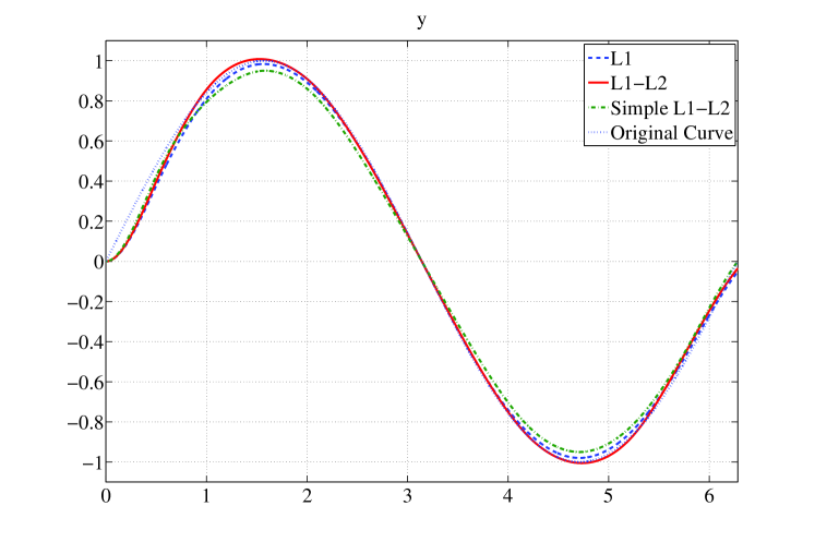
Figure 6. The original curve (dots) and outputs: by $\ell^{2}$-optimal ${\boldsymbol{\theta}}_{2}^{\ast}$ (dash), $\ell^{1}\text{-}\ell^{2}$-optimal ${\boldsymbol{\theta}}_{\text{sparse}}^{\ast}$ (solid), and simple $\ell^{1}\text{-}\ell^{2}$-optimal ${\boldsymbol{\eta}}_{\text{sparse}}^{\ast}$ (dash-dots).

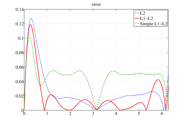
Figure 7. The reconstruction errors: by $\ell^{2}$-optimal ${\boldsymbol{\theta}}_{2}^{\ast}$ (dash), $\ell^{1}\text{-}\ell^{2}$-optimal ${\boldsymbol{\theta}}_{\text{sparse}}^{\ast}$ (solid), and simple $\ell^{1}\text{-}\ell^{2}$-optimal ${\boldsymbol{\eta}}_{\text{sparse}}^{\ast}$ (dash-dots).

The transient responses show relatively large errors because of the phase delay in the plant $P(s)=1/(s+1)^{2}$. Despite of sparsity in ${\boldsymbol{\theta}}_{\text{sparse}}^{\ast}$ and ${\boldsymbol{\eta}}_{\text{sparse}}^{\ast}$, the performances of the reconstructed signals are comparable to that of the $\ell^{2}$-optimal reconstruction by ${\boldsymbol{\theta}}_{2}^{\ast}$. To see the difference between these performances more precisely, we draw the reconstruction errors in Fig. 7. We can see that the errors by ${\boldsymbol{\theta}}_{2}^{\ast}$ and ${\boldsymbol{\theta}}_{\text{sparse}}^{\ast}$ are almost comparable, and the error by ${\boldsymbol{\eta}}_{\text{sparse}}^{\ast}$ is relatively large.

Then we consider quantization. We use the uniform quantizer with step size $0.1$ and simulate the output reconstruction. Table 2 shows the quantized vectors. Fig. 8 shows the reconstruction error under quantization. The errors by the sparse vectors ${\boldsymbol{\theta}}_{\text{sparse}}^{\ast}$ and ${\boldsymbol{\eta}}_{\text{sparse}}^{\ast}$ still remains small while the $\ell^{2}$-optimal reconstruction shows errors affected by quantization. This is because the zero-valued elements in the sparse vectors do not suffer from any quantization distortion.

tbp

Table 2. Quantized vectors

$Q({\boldsymbol{\theta}}_{2}^{\ast})$	$Q({\boldsymbol{\theta}}_{\text{sparse}}^{\ast})$	$Q({\boldsymbol{\eta}}_{\text{sparse}}^{\ast})$	$Q({\boldsymbol{y}}_{\text{ref}})$
9.8	9.7	0.5	0.5
2.8	4.6	0.8	0.9
1.7	0.0	1.0	1.0
1.7	3.0	0.8	0.9
1.0	0.0	0.5	0.5
0.0	0.0	0.0	0.0
-1.0	0.0	-0.5	-0.5
-1.7	-2.9	-0.8	-0.9
-2.0	-0.6	-1.0	-1.0
-2.2	-4.9	-0.8	-0.9
-2.4	0.0	-0.5	-0.5
5.2	4.4	0.0	0.0

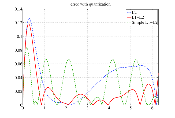
Figure 8. The reconstruction errors with quantization: by $\ell^{2}$-optimal $\hat{{\boldsymbol{\theta}}}_{2}^{\ast}$ (dash), $\ell^{1}\text{-}\ell^{2}$-optimal $\hat{{\boldsymbol{\theta}}}_{\text{sparse}}^{\ast}$ (solid), and simple $\ell^{1}\text{-}\ell^{2}$-optimal $\hat{{\boldsymbol{\eta}}}_{\text{sparse}}^{\ast}$ (dash-dots).

7. Conclusion

In this paper, we have proposed to use sparse representation for command generation in remote control by $\ell^{1}\text{-}\ell^{2}$ optimization. An example illustrates the effectiveness of the proposed method. Future work may include the study of advantages of sparse representation in view of information theory.

References

• [1] A. Beck and M. Teboulle, A fast iterative shrinkage-thresholding algorithm for linear inverse problems, SIAM J. Imaging Sciences, vol. 2, No. 1, 183/202 (2009)
• [2] E. J. Candes and M. B. Wakin, An introduction to compressive sampling, IEEE Signal Processing Mag., vol. 25, 21/30 (2008)
• [3] S. S. Chen, D. L. Donoho, and M. A. Saunders, Atomic decomposition by basis pursuit, SIAM Journal on Sci. Comp., vol. 20, No. 1, pp. 33–61 (1998)
• [4] T. M. Cover and J. A. Thomas, Elements of Information Theory, 2nd edition, Wiley (2006)
• [5] I. Daubechies, M. Defrise, and C. De Mol, An iterative thresholding algorithm for linear inverse problems with a sparsity constraint, Communications on Pure and Applied Mathematics, Vol. 57, No. 11, pp. 1413–1457 (2004)
• [6] M. Egerstedt and C.F. Martin, Control Theoretic Splines, Princeton University Press (2010)
• [7] M. Elad, Sparse and Redundant Representations, Springer (2010)
• [8] M. Elad and A. Bruckstein, A generalized uncertainty principle and sparse representation in pairs of bases, IEEE Trans. Inform. Theory, Vol. 48, No. 9, pp. 2558–2567 (2002)
• [9] R. C. Luo and T. M. Chen, Development of a multibehavior-based mobile robot for remote supervisory control through the Internet, IEEE/ASME Trans. Mechatron., Vol. 5, No. 4 (2000)
• [10] M. Nagahara and D. E. Quevedo, Sparse representation for packetized predictive networked control, IFAC World Congress (2011) (to be presented)
• [11] C. Sayers, Remote Control Robotics, Springer (1999)
• [12] B. Schölkopf and A. J. Smola, Learning with Kernels, The MIT Press (2002)
• [13] S. Sun, M. B. Egerstedt, and C. F. Martin, Control theoretic smoothing splines, IEEE Trans. Automat. Contr. Vol. 45, No. 12, 2271/2279 (2000)
• [14] A. F. T. Winfield and O. E. Holland, The application of wireless local area network technology to the control of mobile robots, Microprocessors and Microsystems, Vol. 23, pp. 597–607 (2000)
• [15] M. Zibulevsky and M. Elad, L1-L2 optimization in signal and image processing, IEEE Signal Processing Mag., Vol. 27, 76/88 (2010)