Direct observation of atomic diffusion in warm rubidium ensembles

Abstract

We present a robust method for measuring diffusion coefficients of warm atoms in buffer gases. Using optical pumping, we manipulate the atomic spin in a thin cylinder inside the cell. Then we observe the spatial spread of optically pumped atoms in time using a camera, which allows us to determine the diffusion coefficient. As an example, we demonstrate measurements of diffusion coefficients of rubidium in neon, krypton and xenon acting as buffer gases. We have determined the normalized (273 K, 760 Torr) diffusion coefficients to be 0.18$\pm 0.03$ cm²/s for neon, 0.07$\pm 0.01$ cm²/s for krypton, and 0.052$\pm 0.006$ cm²/s for xenon.

1 Introduction

Warm atomic ensembles have recently become a very useful tool in modern quantum engineering. The most notable applications include quantum memories (van der Wal et al., 2003; Appel et al., 2008) and quantum repeaters (Duan et al., 2001) that can lead to development of quantum networks (Kimble, 2008). Warm atoms have also been used as a medium for four-wave mixing (McCormick et al., 2008), electromagnetically induced transparency (EIT) (Fleischhauer et al., 2005) and ultraprecise magnetometry (Chalupczak et al., 2012).

While experiments with vapors contained in sealed cells are relatively simple, they are limited by inevitable atomic motion. Typically a buffer gas is used to contain the atoms and make their motion diffusive. In all of the above examples the diffusion rate was among primary performance limiting factors. Its importance has been recognized and its effect on EIT (Shuker et al., 2008; Firstenberg et al., 2008, 2010; Yankelev et al., 2013) and on the Gradient Echo Memory (Glorieux et al., 2012; Higginbottom et al., 2012; Luo et al., 2013) have been studied both experimentally and theoretically.

Prior knowledge of diffusion coefficients enables designing optimal experiments and greatly facilitates the interpretation of the results. However, there is a striking lack of precise measurements of diffusion coefficients in various buffer gases. We believe that the reason for this is unavailability of robust methods. In most cases diffusion coefficients were deduced using methods designed for studying spin-exchange of optically aligned atoms (Franzen, 1959).

The lack of both data and methods motivated us to develop a simple and robust procedure designed specifically to measure the diffusion coefficients. We demonstrate it on an example of diffusion of rubidium in neon, krypton and xenon.

In our method, we pump optically a thin pencil-shaped volume of atoms inside a given cell using a short laser pulse. After the pump pulse ends, we wait for a varying time and let rubidium atoms diffuse. Then we send a pulse from a probe laser in a beam that covers nearly the entire cell. The probe light is virtually unaffected by pumped atoms but absorbed by the unpumped ones. Therefore spatial distribution of the transmitted probe light reveals how far the atoms have travelled between the pump and probe pules and thus provides the diffusion coefficient.

This paper is organized as follows. In section 2 we present a simple model that describes our method. In section 3 we describe in detail our experimental setup. In section 4 we present practical methods for analyzing the data obtained. Section 5 gives the results of our measurements and compares them with theoretical predictions as well as with the results obtained previously. Section 6 concludes the paper.

2 Method

In out method, we register a decrease in optical depth of the atomic sample due to optical pumping $\Delta OD(x,y,t)$ as a function of spatial position $(x,y)$ and the delay $t$ between the pumping and the actual observation. In practice, the difference $\Delta OD$ may be computed by measuring the intensity of light that passes through our cell with $I_{\mathrm{p}}(x,y,t)$ and without optical pumping $I_{\mathrm{np}}(x,y)$. The formula reads:

$$\Delta OD(x,y,t)=\ln\left(\frac{{I_{\mathrm{p}}(x,y,t)}}{I_{\mathrm{np}}(x,y)}\right).$$ (1)

The decrease in optical depth is also proportional to the decrease in density of the atoms in the ground state of the atomic transition to which the probe is coupled, that is $c_{\mathrm{np}}-c_{\mathrm{p}}(x,y,t)$, where $c_{\mathrm{np}}$ stands for the equilibrium density observed without pumping. Since the density $c_{\mathrm{p}}(x,y,t)$ at time $t$ after pump pulse evolves according to the diffusion equation, so does the decrease in the optical depth $\Delta OD(x,y,t)$.

In addition to the diffusion, other mechanisms, such as spin-exchange collisions, may urge the density $c_{\mathrm{p}}(x,y,t)$ towards the steady state value $c_{\mathrm{np}}$. We call the rate of those relaxation processes $\gamma_{0}$ and observe that it is position-independent. Later we incorporate it into data analysis. Moreover, the atoms may relax in collisions with cell walls. In our experiments the observation times $t$ were too short for pumped atoms to reach the side walls. Some portion of the initially pumped volume would reach cell windows, however since the length of the cell is almost 100 times the typical diffusion distance, the boundary effects are negligible.

It is convenient and intuitive to assume that the density $c_{\mathrm{p}}(x,y,t)$ after pumping is $z$-independent, which requires that the pump beam should saturate the absorption in the ensemble. In fact, this assumption is not necessary, as every solution to the 3D diffusion equation (in this case with additional relaxation) can be written as sum of separable solutions, that is $c_{\mathrm{np}}-c_{\mathrm{p}}(x,y,z,t)=\sum_{j}u_{j}(x,y,t)f_{j}(z,t)\exp(-\gamma_{0}t)$, where both $u_{j}(x,y,t)$ and $f_{j}(z,t)$ satisfy the diffusion equation in respective coordinates. Now we integrate over $z$ to finally obtain the decrease in the optical depth $\Delta OD(x,y,t)$, but the integral $\int_{0}^{L}f_{j}(z,t)\mathrm{d}z$ is time-independent, as the relaxation at optical windows is negligible. The optical depth difference will satisfy the 2D diffusion equation with relaxation, as it is now a linear combination of $u_{j}(x,y,t)$ with time-independent coefficients.

By fitting Gaussians to obtained $\Delta OD(x,y,t)$ cross-sections as presented in Fig. 1, we can estimate the diffusion coefficient $D$ using the diffusion rule for the width of fitted Gaussians $\sigma_{x}(t)=\sqrt{{\sigma_{x}(t=0)^{2}+4Dt}}$. A more universal method is presented in Data Analysis section.

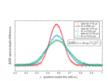
Fig. 1: Typical examples of obtained optical depth difference $\Delta OD(x,y=0,t)$ maps at various times $t$ after pump pulse. Gaussian fits give us widths of these distributions $\sigma_{x}(t)$ as a function of diffusion time.

3 Experimental Setup

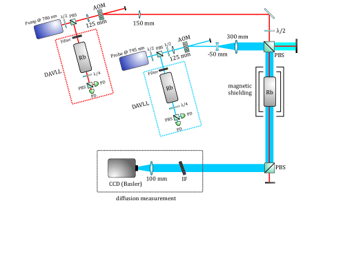
Fig. 2: Schematic of our experimental setup; AOM acousto-optic modulator, DAVLL dichroic atomic vapor laser lock setup (Corwin et al., 1998), PD photodiode, PBS polarizing beam-splitter, Rb rubidium vapor cell, $\lambda/2$ half-wave plate, $\lambda/4$ quarter-wave plate, IF interference filter, CCD charge coupled device camera. Lenses are labeled with their focal lengths.

Fig. 2 presents a schematic of the experimental setup. Both pump and probe lasers are Toptica distributed feedback laser diodes, each frequency stabilized using dichroic atomic vapor spectroscopy (Corwin et al., 1998).

In case of rubidium 87 the pump laser was tuned to $F_{g}=1\rightarrow F_{e}=0,1,2$ transitions on D2 line and the probe laser to $F_{g}=1\rightarrow F_{e}=2$ transition on D1 line. In case of rubidium 85 the pump laser was tuned to $F_{g}=3\rightarrow F_{e}=2,3,4$ transitions on D2 line and the probe laser to $F_{g}=3\rightarrow F_{e}=2,3$ transitions on D1 line. We have found that the stability of the pump laser is important, as the pumping rate needs to be constant, although the laser does not need to be tuned precisely to the center of any transition.

The laser beams are directed onto the acousto-optic modulators (AOM) used to produce the pulse sequence. The beam shaping optics follows. Both beams are collimated and the probe beam is expanded to a desired $1/e^{2}$ waist diameter of about 1 cm, while the pump beam has a waist diameter of 1 mm.

The beams are joined on a polarizing beam splitter (PBS). Half-wave plates before the joining point allow us to control the power of both beams precisely. After the PBS, the beams are parallel and overlap.

Both beams pass through a quartz cell (Precision Glassblowing, 25 mm in diameter, various lengths) filled with isotopically pure rubidium vapor and buffer gas. The vapor cell is placed inside a $\mu$-metal magnetic shielding to avoid pumping alternations due to external magnetic filed. The cell is mounted in flexible aluminum sleeves heated with a bifilar-wound copper coil. Despite the bifilar winding, we have found that it is better to stop the heating for the time of measurement to avoid disturbing the pumping. The holder temperature stabilization is based on the resistance of the coil’s windings.

The vapor temperature is determined by measuring absorption spectrum of the cell and fitting the result with a theoretical curve. We keep the temperature within the $5^{\circ}$C range around $40^{\circ}$C.

After passing through the cell, the pump beam is filtered out by a PBS and an interference filter. We image the inside of the cell on a CCD camera (Basler, scA1400-17fm) with a single lens. Magnification of this optical system was both calculated and measured with a cell replaced by a reference target. These two methods led to consistent results, showing that camera’s pixel pitch correspond to a $59\pm 2$ $\mu$m distance inside the cell.

The camera is triggered synchronously with laser pulses. We use minimal shutter duration (40 $\mu$s) to minimize the background coming mainly from scattering on the AOMs. In addition, by controlling the time when shutter opens, we minimize the amount of pump light registered by the camera. We achieved a relatively low background level, dominated by the electronic offset. It was sufficient to subtract constant background intensity from each image frame.

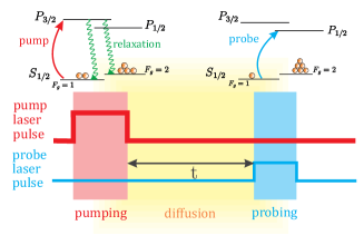
Fig. 3: Light pulse sequence we use in our experiment. The top line represents the pump laser tuned to rubidium D2 line and the bottom line represents the probe laser tuned to D1 line. On the energy level diagrams (in this case of rubidium 87 atom) we show how the optical pumping influences populations: during pumping on the left and during probing on the right. Wavy arrows represent relaxation mainly due to spontaneous emission.

The pulse sequence is represented schematically in Fig. 3. To measure the reference intensity of the probe light $I_{\mathrm{np}}(x,y)$, we send a $0.4$ $\mu$s probe pulse alone and image the beam shape after passing through the cell. To measure the probe light intensity with the optical pumping present $I_{\mathrm{p}}(x,y,t)$, first we apply a $0.5$ $\mu$s pump pulse and then wait for a varying time $t$ and apply a $0.4$ $\mu$s probe pulse. The initial $\Delta OD(x,y,t=0)$ is diffused only slightly due to the short pump pulse. The unsaturated absorption of the pump light was about 70%, but saturation effects caused half of the pump pulse to be transmitted through the cell. It resulted in optical pumping being weakly dependent on $z$. The delay time $t$ varies from 1 to 150 $\mu$s. Each collected image of the probe beam is averaged over 50 measurements, and the entire collection sequence for all delays $t$ is repeated 10 times. This allows us to average over both long-term (min) and short-term (ms) fluctuations. The data collection rate is limited by the 40 Hz frame rate of the camera.

4 Data Analysis

The initial shape of the pumped region is not easily described analytically, therefore we have elected to use a data analysis method that can deal with arbitrary functions. It is based on solving the diffusion equation in the spatial-frequency Fourier domain, which is more general than a Gaussian fit from Fig. 1. A similar method has previously been used in studies of fluorescence redistribution after photobleaching (Tsay and Jacobson, 1991). Let us define the spatial Fourier transform of the decrease of optical depths of the atomic sample due to optical pumping $\Delta OD(x,y,t)$ as:

$$\mathcal{{F}}\{\Delta OD\}(k_{x},k_{y},t)=\\ =\frac{{1}}{2\pi}\iint\mathrm{d}x\mathrm{d}y\Delta{OD}(x,y,t)\exp(-ik_{x}x-ik_{y}y).$$ (2)

As we discussed in Method section the $z$-dependence of atomic density can be separated and $\Delta OD(x,y,t)$ becomes a linear combination of functions satisfying 2D diffusion equation with relaxation, so the time evolution of this Fourier transform due to diffusion takes on a simple form

$$\mathcal{\mathcal{{F}}}\{\Delta OD\}(k_{x},k_{y},t)=\\ =\mathcal{{F}}\{\Delta OD\}(k_{x},k_{y},0)\exp(-(\underbrace{{\gamma_{0}+D(k_{x}^{2}+k_{y}^{2})}}_{\gamma({\bf k})})t).$$ (3)

This solution tells us that a component of optical depth difference having a certain spatial periodicity given by $k_{x}$ and $k_{y}$ (that may be also called spatial frequencies) decays exponentially at a rate

$$\gamma(k_{x},k_{y})=\gamma_{0}+D(k_{x}^{2}+k_{y}^{2}).$$ (4)

The procedure of data analysis according to the above equations is as follows. Having measured optical depths differences $\Delta OD(x,y,t)$ for various delay times $t$, we perform a numerical Fourier transform of each map and get $\mathcal{\mathcal{{F}}}\{\Delta OD\}(k_{x},k_{y},t)$ for different delay times $t$.

Next, for each $\mathbf{k}=(k_{x,}k_{y})$ we fit a simple exponential decay model to the absolute amplitude of a component of the optical depth decrease with a given spatial periodicity. In practice this is possible only for components of high enough amplitudes, that is for $|\mathbf{k}|$ smaller than the inverse pump beam width. The fit result is the decay rate as a function of spatial periodicity $\gamma(\mathbf{k})$. Examplary decay fits for various spatial wavevectors $\mathbf{k}$ are presented in Fig. 4. As this decay rate should only depend on the length of $\mathbf{k}$ vector, we perform an angular averaging procedure to obtain a one-variable function $\gamma(|\mathbf{k}|)$. Finally, we use the relation for the decay rate $\gamma(|\mathbf{k}|)=\gamma_{0}+D|\mathbf{k}|^{2}$ that comes from the diffusion equation. We fit a parabola to the previously computed $\gamma(|\mathbf{k}|)$ dependence and retrieve the diffusion coefficient $D$. Examplary fits for various Rb cells we used are presented in Fig. 5.

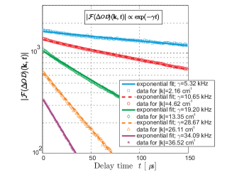
Fig. 4: Examplary exponential decays of $\mathcal{{F}}\{\Delta OD\}(|\mathbf{k}|,t)$ with time between pump and probe, for various components with spatial wavevectors$\mathbf{k}$ in the image of optical depth decrease $\Delta{OD}(x,y,t)$. Data for ⁸⁵Rb cell with 5 Torr of neon.

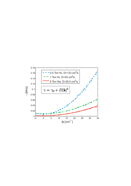
Fig. 5: Quadratic fits of the decay rate $\gamma(|\mathbf{k}|)$ as a function of spatial wavevector $\mathbf{k}$ to the data obtained in the Fourier procedure of data analysis, as in Fig.4.

5 Results

Table 1: Measured diffusion coefficients, normalized diffusion coefficients obtained from our measurements, theoretical predictions based on the Chapman-Enskog formula, and some previous results of the diffusion coefficients measurements.

Cell (buffer gas, Rb isotope)	$D$ [cm2/s] (40∘C)	$D_{\circ}$ (this paper) [cm2/s]		$D_{\circ}$ (theory) [cm2/s]	$D_{\circ}$ (previous results) [cm2/s]
Ne 5 Torr, 85Rb	$29.5\pm 1.0$	0.18$\pm$0.02	0.18$\pm 0.03$	0.145$\pm 0.01$	0.2 (Chrapkiewicz et al., 2014), 0.11 (Shuker et al., 2008), 0.18 (Vanier et al., 1974), 0.31 (Franzen, 1959; Arditi and Carver, 1964), 0.48 (Franz, 1965)
Ne 2 Torr, 87Rb, paraf.	$62.0\pm 0.8$	0.15$\pm$0.02
Ne 100 Torr, 85Rb	$1.69\pm 0.04$	0.21$\pm$0.03
Ne 50 Torr, 87Rb	$2.70\pm 0.04$	0.17$\pm$0.02
Kr 1 Torr, 87Rb	$71\pm 2$	0.08$\pm$0.01	0.07$\pm 0.01$	0.065$\pm 0.005$	0.068 (Chrapkiewicz et al., 2014), 0.1 (Bouchiat, 1972), 0.04 (Higginbottom et al., 2012)
Kr 1 Torr, 87Rb, paraf.	$45\pm 2$	0.06$\pm$0.01
Kr 0.5 Torr, 87Rb	$133\pm 4$	0.08$\pm$0.01
Xe 1 Torr, 87Rb, paraf.	$43\pm 1$	0.052$\pm 0.006$		0.055$\pm 0.005$	0.057 (Chrapkiewicz et al., 2014)

The presented results were obtained using the Fourier method described above. Special care was taken to ensure validity of each step, including verification of rotational symmetry of $\gamma(\mathbf{k})$, which allowed us to proceed with angular averaging to obtain $\gamma(|\mathbf{k}|)$. We noticed that good alignement was critical when ensuring that the spread of values of $\gamma(\mathbf{k})$ for a given $|\mathbf{k}|$ was small. Optimizing the setup resulted in this spread being much smaller than the uncertainty coming from each exponential fit, but both error sources were taken into account when calculating uncertainties.

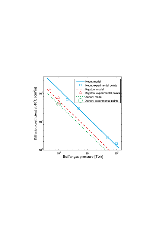
Fig. 6: Summary of obtained diffusion coefficients of rubidium in various buffer gases compared with inverse relation to buffer gas pressure predicted by the Chapman-Enskog model.

Table 1 ($D$, second column) contains diffusion coefficients at 40^∘C of rubidium in various cells, containing neon, krypton or xenon. In the Fig. 6 we see that the diffusion coefficient scales with inverse of vapor gas pressure as expected (Cussler, 2009) over a broad range of buffer gas pressures, especially for neon. In this figure we also include curves representing model behaviour. The diffusion coefficients we measured in two cells with 1 Torr krypton differ much more than expected. We believe that this could be due to different true quantity of gas contained in those cells due to variations in the seal-off process. Most likely the pressure was measured at significantly different temperatures of the cell bodies. Another reason could be significant evaporation of the paraffin coating which was present only in one cell as chemicals such as volatile hydrocarbons present in the coating could slow down the diffusion when in gaseous state.

To our knowledge, our group has been the first one to measure directly the diffusion coefficient of rubidium in xenon. The result we present here confirms the previously measured value (Chrapkiewicz et al., 2014).

We scaled the results to normal conditions (760 Torr pressure and $0^{\circ}$C temperature) for Ne, Kr and Xe using Chapman-Enskog formula (Cussler, 2009). We inferred uncertainties of normalized diffusion coefficient for neon and krypton from the spread of experimental results. In case of xenon we attribute the uncertainty of the result to the uncertainty of buffer gas pressure. Note that unnormalized diffusion coefficient for each cell are measured much more accurately. Values of collision integrals at different temperatures were obtained according to the procedure described in Ref. (Cussler, 2009). Required collisional parameters were taken from Refs. (Ghatee and Niroomand-Hosseini, 2007) and (Gibble and Gallagher, 1991). The ideal gas model was used for the relation between pressure of the buffer gas and temperature. We believe that using the Chapman-Enskog formula and normalized results we present here, it is possible to calculate the diffusion coefficient of rubidium in Ne, Kr or Xe at an arbitrary pressure or temperature.

In the Table 1 we compare our normalized experimental results ($D_{\circ}$, third column) with theoretical predictions based on Chapman-Enskog formula and studies of atomic collisions ($D_{\circ}$, fourth column). Our results display satisfactory conformity with theoretical predictions. Note that both the normalization we perform and the theoretical predictions are based on a fundamentally approximate theory, as the Chapman-Enskog formula comes from an approximate solution of the Boltzmann equation and requires various parameters that were calculated indirectly.

The results we present here differ significantly from some of the previous results (last column in table 1), however we believe ours are more reliable for several reasons. Firstly, the results of this paper agree with the results we obtained using the same cells (Chrapkiewicz et al., 2014) but a completely different method. Secondly, the former methods relied on measuring the relaxation of the atomic spin alignments a function of gas pressure to retrieve both the diffusion coefficient and the spin-exchange rates (Franzen, 1959).

6 Conclusions

We have presented a robust and simple method for measuring the diffusion coefficients of warm atoms in buffer gases. Our method might be used in all systems where the phenomenon of optical pumping occurs. We have shown that observing the spread of a optically pumped region by applying a pulsed probe beam and imaging it on a camera is sufficient to determine the diffusion coefficient of the system. The data analysis involved Fourier transforming of measured optical depth differences and finding decay rates for components of different spatial periodicity. This approach is robust and provides opportunities for data consistency checks at various calculation stages.

Our method can be easily used to measure diffusion in countless physical systems and is easy to implement. In principle one laser could be sufficient for both pump and probe pulses.

As a demonstration we have measured the diffusion coefficients of rubidium in neon, krypton and xenon. Our results are consistent with both theoretical predictions and previous results. We have also found the presented method very useful when it comes to characterizing various sealed cells with rubidium and a buffer gas. Notably, it is capable of capturing wide range of diffusion coefficients, of at least two orders of magnitude.

We believe that our measurements will enable greater control and better design of experiments with warm rubidium ensembles. In particular we note that krypton and xenon appear to be very good buffer gases for modern quantum applications; yet, they have scarcely been used so far. Apart from us only one group has utilized krypton (Hosseini et al., 2009), while xenon has been used only by us (Chrapkiewicz et al., 2014).

To our knowledge our group has been the first one to measure actually the diffusion coefficient of rubidium in xenon, with this paper confirming Ref. (Chrapkiewicz et al., 2014). Given the recent applications of hyperpolarized ¹²⁹Xe in medical imaging, we hope that the precise value of this diffusion coefficient will help optimize setups like the one presented in Ref. (Fink et al., 2005).