Critical behavior of the exclusive queueing process

Abstract

The exclusive queueing process (EQP) is a generalization of the classical M/M/1 queue. It is equivalent to a totally asymmetric exclusion process (TASEP) of varying length. Here we consider two discrete-time versions of the EQP with parallel and backward-sequential update rules. The phase diagram (with respect to the arrival probability $\alpha$ and the service probability $\beta$) is divided into two phases corresponding to divergence and convergence of the system length. We investigate the behavior on the critical line separating these phases. For both update rules, we find diffusive behavior for small service probability ($\beta<\beta_{c}$). However, for $\beta>\beta_{c}$ it becomes sub-diffusive and nonuniversal: the critical exponents characterizing the divergence of the system length and the number of customers are found to depend on the update rule. For the backward-update case, they also depend on the hopping parameter $p$, and remain finite when $p$ is large, indicating a first order transition.

I Introduction

The M/M/1 queueing process describes the dynamics of a queue which is specified by the arrival probability $\alpha$ and service probability $\beta$ ref:Medhi ; ref:Saaty . It has two phases separated by the critical line $\alpha=\beta$: for $\alpha>\beta$ the length of the queue diverges whereas it converges for $\alpha<\beta$. In the M/M/1 queueing process, the internal structure of the queue is not considered, i.e. the queue has density 1 everywhere.

The exclusive queueing process (EQP) is a simple generalization of this classical M/M/1 queueing process. It was introduced to impose excluded-volume effect such that the internal structure of queues is taken into account ref:A ; ref:YTJN ; ref:AY . Customers (i.e. “particles”) move according to the rules of the totally asymmetric simple exclusion process (TASEP), which is a paradigmatic model of interacting many-particle systems far from equilibrium ref:D ; ref:SCN . The EQP can be regarded as a TASEP with variable system length. Some TASEPs or related systems with a variable length have been studied, especially in the context of biological applications, e.g. to the growth of hyphae, microtubules or bacterial flagellar filaments ref:SEPR ; ref:SE ; ref:ES ; ref:DMP ; ref:JEK ; ref:MRF ; ref:SS .

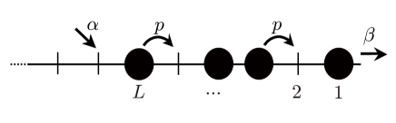
Figure 1: Dynamics of the exclusive queueing process (EQP).

The EQP is defined on a semi-infinite one-dimensional lattice, where the sites are labeled by natural numbers from right to left, see fig. 1. Each site $j$ is either empty or occupied by a customer. The system length $L$ is defined as the position of the leftmost occupied site. It is in general different from the number $N$ of customers which have unit length in contrast to the M/M/1 queue where one has always $L=N$. Due to the exclusion principle, customers move forward with probability $p$ in each time step only if the preceding site is unoccupied. A new customer enters the system at the end of the queue, i.e. at the site $L+1$ next to the leftmost occupied site, with probability $\alpha$. The customer at the rightmost site $j=1$ gets service with probability $\beta$ and is removed from the system.

We need to specify an update rule to fully define the dynamics of the EQP. Here we consider parallel and backward-sequential update rules. In the EQP with parallel update (parallel EQP), all sites are updated simultaneously. In the EQP with backward-sequential update (backward EQP), first a customer arrives with probability $\alpha$, and the customer at the right end ($j=1$) is extracted with probability $\beta$ (if it exists). Then starting from the rightmost customer and going sequentially to the left up to the leftmost customer, the system is updated according to the rules of the TASEP (see ref:AS3 for more details) One can also consider the EQP with continuous time ref:A . Relations among the two discrete-time EQPs, the continuous-time EQP, and some special cases have been studied in ref:AS3 .

Exact stationary states for the continuous-time and parallel EQPs have been found ref:A ; ref:AY . However, obtaining an exact “dynamical state” (time-dependent solution) was not possible so far except for deterministic hopping $p=1$ ref:AS1 ; ref:AS2 . Thus we rely on Monte Carlo simulations to investigate time-dependent properties of the EQPs. In this work, we focus on critical properties, i.e. the behavior of the system length $L$ and the number $N$ of customers on the critical line of the EQP. Getting reliable results then requires averaging over a large number of samples and long times.

II Critical line

The critical line that separates the convergent and divergent phases in the usual M/M/1 queueing process is simply $\alpha=\beta$. In the EQP case, it is modified depending on the update rule ref:AS1 ; ref:AS3 : for the parallel EQP,

$$\alpha_{c}=\begin{cases}\frac{\beta(p-\beta)}{p-\beta^{2}}&\qquad\text{for\ }\beta\leq\beta_{c},\\ \frac{1-\sqrt{1-p}}{2}&\qquad\text{for\ }\beta>\beta_{c},\end{cases}$$ (1)

and for the backward EQP,

$$\alpha_{c}=\begin{cases}\frac{\beta(p-\beta)}{p(1-\beta)}&\qquad\text{for\ }\beta\leq\beta_{c},\\ \frac{(1-\sqrt{1-p})^{2}}{p}&\qquad\text{for\ }\beta>\beta_{c},\end{cases}$$ (2)

where

$$\beta_{c}=1-\sqrt{1-p}$$ (3)

is independent of the update rule. The form for $\alpha_{c}$ corresponds to the outflow of customers, and thus the time-dependent behavior of the average number of customers is well expressed as ref:AS1

$$\langle N_{t}\rangle\sim(\alpha-\alpha_{c})t$$ (4)

which is the asymptotic form in the divergent phase ($\alpha>\alpha_{c}$). Equation (4) is true only for $t\lesssim(\alpha_{c}-\alpha)/\langle N_{0}\rangle$ in the convergent phase ($\alpha<\alpha_{c}$) where $\langle N_{t}\rangle$ converges to a stationary value. Similarly, the length $\langle L_{t}\rangle$ of the system converges to a stationary value ($\alpha>\alpha_{c}$) or diverges linearly in $t$ ($\alpha<\alpha_{c}$).

The results (1) and (2) suggest a division of the phase diagram into four phases (fig. 2) by distinguishing between maximal current and high density phases ref:AS1 . The divergent phase is further divided into up to five subphases according to the shape of the density profile. The pair of coefficients (or growth velocities) $\bigl{(}\frac{\langle N_{t}\rangle}{t}$, $\frac{\langle L_{t}\rangle}{t}\bigr{)}$ has a different expression in each subphase ref:AS3 .

Figure 2: Phase diagram of the parallel EQP. The phase diagram of the backward EQP is qualitatively the same, with $\frac{1-\sqrt{1-p}}{2}$ replaced by $\frac{(1-\sqrt{1-p})^{2}}{p}$. The phases with diverging length are indicated by the extension “-D” and convergent phases by “-C”. The maximal current (MC) and high-density (HD) phases are distinguished by the form of $\alpha_{c}$ in (1) and (2).

In our previous work ref:AS3 , we have observed the behavior

$$\langle X_{t}\rangle=O\left(t^{\gamma_{X}}\right)$$ (5)

of the system length ($X=L$) and the number of customers ($X=N$) just on the critical line with non-trivial growth exponents $\gamma_{X}$. Since clearly $\gamma_{X}=0$ in the convergent phase and $\gamma_{X}=1$ in the divergent phase, it is natural to expect $0\leq\gamma_{X}\leq 1$ on the critical line. This is indeed confirmed by the simulations, see figs. 3, 4. (In fig.  4, we rescale the service probability $\beta$ such that $\tilde{\beta}=0,0.5$ and 1 correspond to $\beta=0,\beta_{c}$ and 1, respectively.)

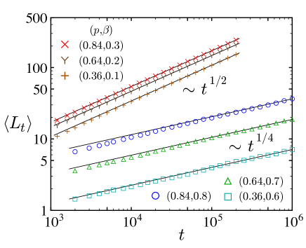
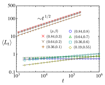
Figure 3: Log-log plots of the average system length $\langle L_{t}\rangle$ for the parallel (top) and backward (bottom) EQPs. Simulations were averaged over $10^{5}$ and $10^{6}$ samples for the curved part ($\times$, Y, $+$) and the straight part ($\bigcirc,\triangle,\square,\Diamond$) of the critical line, respectively. The data are in good agreement with the power law behavior (5). To obtain the fitting lines, we fixed $\gamma_{L}=\frac{1}{2}$ or $\frac{1}{4}$ except for the backward case on the straight part, where the exponents have been estimated from eq. (13).

Here, we will examine the exponents systematically, and find that they exhibit different behavior depending on parts of the critical line (curved part $\beta<\beta_{c}$, i.e. the phase boundary between the high-density subphases, or straight part $\beta>\beta_{c}$, i.e. the phase boundary between the maximal-current subphases). To obtain reliable results, we take averages over a large number ($10^{5}$, $10^{6}$ or more) of simulation samples with up to $10^{6}$ time steps. In particular for the backward case, fluctuations are strong and a large number of samples is required to determine the exponents accurately. As initial condition ($t=0$), simulations are started from an empty lattice where no customers are present in the system.

III On the curved part

For the case of deterministic hopping case $p=1$ rigorous results exist ref:YTJN ; ref:AS1 ; ref:AS2 . In this case, $\beta_{c}=1$ and the MC-C and MC-D phases vanish from the phase diagram. For the parallel EQP one has $L\neq N$ due to the exclusion principle and a time-dependent solution can be obtained in matrix product form ref:AS2 . On the other hand, the backward EQP with $p=1$ reduces to the usual M/M/1 queue with $L=N$. On the critical line, i.e.

$$\alpha=\begin{cases}\frac{\beta}{1+\beta}&\qquad({\rm parallel}),\\ \beta&\qquad({\rm backward}),\end{cases}$$ (6)

the system length and the number of customers exhibit diffusive behavior:

$$\langle L_{t}\rangle=C_{L}\sqrt{t}+o(\sqrt{t}),\qquad\langle N_{t}\rangle=C_{N}\sqrt{t}+o(\sqrt{t}),$$ (7)

where the coefficients depend on the update rules,

$$C_{L}=\left\{\begin{array}[]{ll}2\sqrt{\frac{\beta(1-\alpha)}{\pi}}&\ ({\rm parallel}),\\ 2\sqrt{\frac{\beta(1-\beta)}{\pi}}&\ ({\rm backward}),\end{array}\right.\qquad C_{N}=\rho\,C_{L},$$ (10)

with the average density

$$\rho=\begin{cases}\frac{1}{1+\beta}&\qquad({\rm parallel)},\\ 1&\qquad({\rm backward}).\end{cases}$$ (11)

Note that since $\alpha$ and $\beta$ are related by equation (6), one can express the coefficients in various ways.

We denote the probability that site $j$ is occupied by a customer at time $t$ by $\rho_{jt}$. For the deterministic hopping case $p=1$, this density profile can be expressed by the complementary error function ${\rm erfc}(x)=\int^{\infty}_{x}e^{-y^{2}}dy$ as

$$\rho_{x\sqrt{t},t}\to\rho\ {\rm erfc}\left(\frac{\sqrt{\pi}}{C_{L}}\right)\qquad(t\to\infty).$$ (12)

We now turn to the behavior on the curved part for general $p$. The exponents $\gamma_{X}$ ($X=L,N$) are estimated from the simulation data by

$$\ln\frac{\langle X_{t}\rangle}{\langle X_{t/10}\rangle}\Big{/}{\ln 10}$$ (13)

which approaches the true exponent $\gamma_{X}$ for $t\to\infty$.

The results in fig. 4 strongly indicate that on the curved part ($\beta<\beta_{c}$, i.e. $\tilde{\beta}<0.5$) the exponents are given by

$$\gamma_{X}=\frac{1}{2}\,,$$ (14)

i.e. diffusive behavior as in the deterministic case $p=1$.

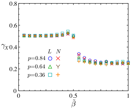
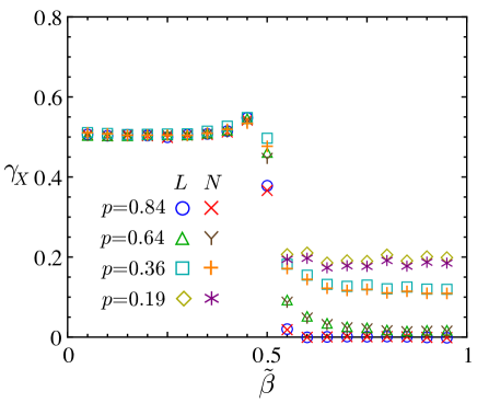
Figure 4: Growth exponents $\gamma_{X}$ for the parallel (top) and backward (bottom) EQPs based on estimates from eq. (13). The parameter $\beta$ has been rescaled as $\tilde{\beta}=\frac{\beta}{2\beta_{c}}$ (for $\beta\leq\beta_{c}),\frac{\beta+1-2\beta_{c}}{2(1-\beta_{c})}$ (for $\beta>\beta_{c})$ for better visibility. The separation of the straight and the curved part of the critical line is then located at $\tilde{\beta}=\frac{1}{2}$. The hopping parameter is chosen as $p=0.84,0.64,0.36$ (additionally $p=0.19$ for $\tilde{\beta}>1/2$ in the backward case). Simulations up to $t\leq 2\times 10^{5}$ and $t\leq 10^{6}$ for $\tilde{\beta}\leq 0.5$ and $\tilde{\beta}>0.5$, respectively, have been used with averaging over $10^{5}$ samples. On the straight part for the backward case, averaging was done over $(2\tilde{\beta}-1)\times 10^{6}$ (for $\tilde{\beta}<0.75)$ or $10^{6}$ (for $\tilde{\beta}\geq 0.75)$ samples due to the strong fluctuations. Clearly the exponents are different for $\tilde{\beta}<0.5$ and $\tilde{\beta}>0.5$.

Next we estimate the coefficients $C_{X}$. Interestingly, simulation data for $\frac{\langle L_{t}\rangle}{\sqrt{t}}$ are in good agreement with the exact result (10) for $C_{L}$ in the deterministic case $p=1$ except near $\beta_{c}$ (fig. 5). In a similar way, the form (10) for $\frac{\langle N_{t}\rangle}{\sqrt{t}}$ with a modification of the mean density as

$$\rho=\begin{cases}\frac{p-\beta}{p-\beta^{2}}&\qquad({\rm parallel}),\\ \frac{p-\beta}{p(1-\beta)}&\qquad({\rm backward}),\end{cases}$$ (15)

fits simulation results well (fig. 5). Furthermore the form (12) gives a good expression for rescaled density profiles (fig. 6).

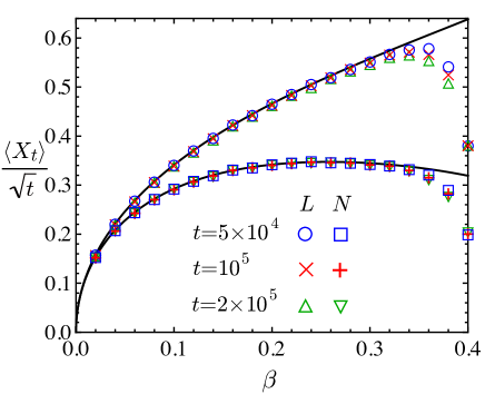
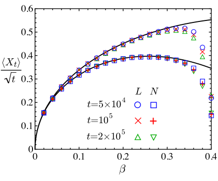
Figure 5: The coefficients $C_{X}=\frac{\langle X_{t}\rangle}{\sqrt{t}}$ ($X=L,N$) on the curved part of the critical line for the parallel (top) and backward (bottom) EQPs. The hopping probability is chosen as $p=0.64$, where $\beta_{c}=0.4$. The markers are plotted by averaging $10^{5}$ simulation samples. We observe that they agree with $C_{L}$ and $C_{N}$ defined by eqs. (10) and (15) (full lines) when $p$ is small.

These facts imply that the EQPs on the critical line are described by noninteracting random walkers hopping rightward or leftward with the same probability $\frac{\pi}{4}C^{2}_{L}$. This is exactly true for the deterministic case $p=1$ ref:AS2 .

In fig. 5, we observe that the finite-time effects become larger as $\beta\nearrow\beta_{c}$, i.e. $\langle X_{t}\rangle/\sqrt{t}$ approaches $C_{X}$ more slowly. This effect can also be observed on the level of the exponents, see fig. 7. We observe that the exponents $\gamma_{L}$ and $\gamma_{N}$ are shifted upward near $\beta_{c}$. Fig. 7 also shows the exponent $\gamma_{\rho}$ of the mean density which is defined by

$$\frac{\langle N_{t}\rangle}{\langle L_{t}\rangle}-\rho=O(t^{-\gamma_{\rho}})$$ (16)

with the limit density (15). It can be estimated by using a formula, which is similar to (13),

$$\ln\frac{\langle N_{10t}\rangle/\langle L_{10t}\rangle-\rho}{\langle N_{t}\rangle/\langle L_{t}\rangle-\rho}\Big{/}{\ln 10}\,.$$ (17)

This exponent is expected to be identical to the two growth exponents $\gamma_{L}$ and $\gamma_{N}$, but the finite-time effect shifts it downward near $\beta_{c}$.

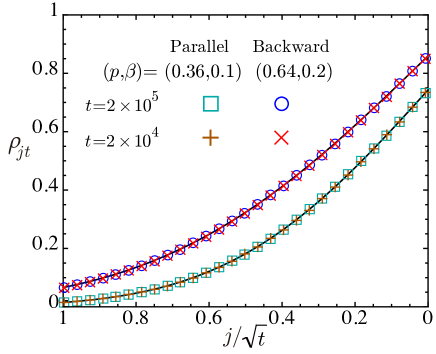
Figure 6: The rescaled density profiles on the curved part of the critical line for the parallel and backward EQPs. The plots were obtained by averaging $10^{5}$ simulation samples. They agree with the lines corresponding to (12) with (10) and (15).

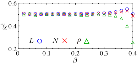
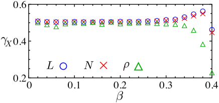
Figure 7: The exponents $\gamma_{X}$ ($X=L,N,\rho$) for the parallel (top) and backward (bottom) EQPs on the curved part of the critical line with $p=0.64$. We applied eqs. (13) and (17) to $10^{5}$ samples up to $t=2\times 10^{5}$ for the estimations.

IV On the straight line

We first consider the parallel case. The top graph of fig. 4 shows the exponents $\gamma_{L}$ and $\gamma_{N}$ for the parallel update. It indicates subdiffusive behavior for $\beta>\beta_{c}$, i.e. $\tilde{\beta}>0.5$. We expect $\gamma_{L}=\gamma_{N}$ so that the total density $\rho_{\rm tot}=\langle N_{t}\rangle/\langle L_{t}\rangle$ reaches the finite value

$$\rho=\frac{1}{2}\qquad({\rm parallel}),$$ (18)

which corresponds to the density of the maximal current ref:RSSS . Although we observe a tendency that $\gamma_{L}$ is slightly larger than $\gamma_{N}$, this can be considered to be a systematic finite-size effect.

The results shown in the top graph of fig. 4 are compatible with universal behavior with the exponents

$$\gamma_{L}=\gamma_{N}=\frac{1}{4}$$ (19)

for the parallel case. This is further supported by fig. 8 where $\gamma_{X}$ are shown with $\beta=(4+\beta_{c})/5$ and various values of the hopping probability $p$. Furthermore the exponent for the mean density (16) is expected to be identical to those for $L$ and $N$:

$$\gamma_{L}=\gamma_{N}=\gamma_{\rho}\,.$$ (20)

For the curved part, we have seen that the behavior is well described by a symmetric random walk model. We expect that the exponent $\frac{1}{4}$ will also be understood by mapping to a simple model, which we leave as an open problem.

Let us turn to the straight part in the backward case ($\tilde{\beta}>0.5$ in the bottom graph of fig. 4). For $\gamma_{\rho}$, we use eq. (17) with

$$\rho=\frac{1-\sqrt{1-p}}{p}\qquad({\rm backward}).$$ (21)

Surprisingly the critical behavior turns out to be rather different from that for the parallel case. Although the exponents $\gamma_{X}$ ($X=L,N,\rho$) are identical to each other (see eq. (20)) for each choice of the parameters, they depend on $p$ (but are independent of $\beta$) and thus the behavior on the straight part is nonuniversal.

When $p$ is small, $L$ and $N$ seem to continue to grow with a power law, see the bottom graph of fig. 8. From the top graph of fig. 8, we find $\gamma_{X}\to\frac{1}{4}$ as $p\to 0$, which matches the exponent for the parallel case. When $p$ is large, we cannot find conclusive evidence for a divergence of $L$ and $N$, see again the bottom graph of fig. 8. Note that in the limit $p\to 1$ (usual M/M/1 case) the straight line part in the phase diagram shrinks to a point $\alpha=\beta=1$. There we can easily show that only the empty chain is realized, i.e. $\langle L_{t}\rangle=0$, which matches the results for large $p$. This property is different from the parallel case, i.e. the straight line shrinks to just the point $(\alpha,\beta)=(0.5,1)$ in the limit $p\to 1$, where $L$ grows infinitely ref:AS2 .

Assuming that $\gamma_{X}$ takes non-zero values when $p$ is small, and $\gamma_{X}=0$ when $p$ is large, there exists a point $p_{c}\approx 0.7$ such that

$$\gamma_{X}\begin{cases}>0&\qquad\text{for }p<p_{c},\\ =0&\qquad\text{for }p\geq p_{c}.\end{cases}$$ (22)

The exponent $\gamma_{L}=0$ ($p\geq p_{c}$) indicates that the transition from the convergent to the divergent phase is of first order, which can be seen more clearly by introducing

$$m=\lim_{t\to\infty}\langle L_{t}\rangle^{-1}$$ (23)

as an order parameter. In the divergent phase this parameter vanishes ($m=0$) whereas it stays finite in the convergent phase ($m>0$). On the critical line with $\beta>\beta_{c}$ and $p\geq p_{c}$, it takes nonzero values so that $m$ changes discontinuously in passing through the critical line. Although eq. (21) can be considered as the limit of the mean density for $p<p_{c}$, this is no longer true for $p\geq p_{c}$ where $\lim_{t\to\infty}\frac{\langle N_{t}\rangle}{\langle L_{t}\rangle}\neq\rho$.

Other scenarios are possible. For example, $L$ and $N$ could converge even for small $p$, but with an extremely long relaxation time. Another possibility is that $L$ and $N$ always diverge with extremely small but nonzero exponents $\gamma_{X}$ or more slowly than a power law, e.g. $\langle X_{t}\rangle=O(\ln t)$ which has been found in a reverse-biased exclusion process with varying length ref:SS . However, we could not confirm these scenarios, and eq. (22) is the most reasonable interpretation of our simulation results ($t\lesssim 10^{6}$).

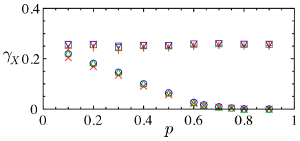
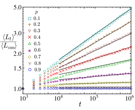
Figure 8: (Top) the exponents $\gamma_{X}$ on the straight part of the critical lines of the parallel ($X=L(\square),N(+),\rho(\bigtriangledown)$) and backward ($X=L(\bigcirc),N(\times),\rho(\bigtriangleup)$) EQPs. (Bottom) log-log plots of the average system length (normalized by $\langle L_{10^{3}}\rangle$ for better visibility) on the straight part of the critical line of the backward EQP. We have set $\beta=(\beta_{c}+4)/5$ with various values of $p$. We applied eqs. (13) and (17) to $10^{6}$ (parallel) and $5\times 10^{6}$ (backward) samples up to $t=10^{6}$ for the estimations. with $\beta=(\beta_{c}+4)/5$.

V At the multicritical point

We lastly examine the behavior at the multicritical point $\beta=\beta_{c}$ where the straight and curved parts of the critical line meet, see fig. 9. For the parallel EQP, we expect diffusive behavior $\gamma_{L}=\gamma_{N}=\frac{1}{2}$ as found on the curved part. However, the exponent for $\rho$ is not identical to them, i.e. $\gamma_{\rho}=\frac{1}{4}$ as on the straight part, so that (10) and (12) are not expected to be valid at the multicritical point.

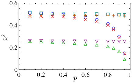
Figure 9: The exponents $\gamma_{X}$ at the multicritical point $(\alpha,\beta)=(\alpha_{c},\beta_{c})$ of the parallel ($X=L(\square),N(+),\rho(\bigtriangledown)$) and backward ($X=L(\bigcirc),N(\times),\rho(\bigtriangleup)$) EQPs with $\beta=\beta_{c}$. We applied eqs. (13) and (17) to $10^{5}$ simulation samples up to $t=2\times 10^{5}$ for the estimations.

In the backward case, the exponents again depend on $p$. For small values of $p$, the exponents are almost the same as in the parallel case, whereas they become smaller as $p\to 1$. However, the dependences of $\gamma_{\rho}$ on $p$ at the multicritical point and on the straight part are different, compare the plot markers $\triangle$ of figs. 8, 9.

VI Summary

We have investigated the EQP, which is characterized by three parameters (arrival probability $\alpha$, service probability $\beta$ and hopping probability $p$), with parallel and backward-sequential update rules. In the $\alpha$-$\beta$ plane, phases of divergent and convergent system length $L$ and customer number $N$ are separated by a critical line which consists of a curved part for $\beta<\beta_{c}$ and a straight-line part for $\beta>\beta_{c}$. Based on Monte Carlo simulations, we have shown that on this critical line the growth exponents $\gamma_{X}$ ($X=L,N$) are smaller than 1, the value in the divergent phase ref:AS1 . We introduced the exponent $\gamma_{\rho}$ for the mean density, and we find generically $\gamma_{L}=\gamma_{N}=\gamma_{\rho}$.

More precisely, we find diffusive behavior $\gamma_{X}=\frac{1}{2}$ ($X=L,N,\rho$) on the curved part ($\beta<\beta_{c}$) of the critical line, which is independent of the update rule. Based on exact results in limiting cases, we also conjectured the coefficients (10) and the asymptotic form (12) of the rescaled density profile, which agree well with the simulation results.

On the straight part ($\beta>\beta_{c}$) of the critical line, the situation is not so simple. First of all, the behavior clearly depends on the update rule. For the parallel case, the exponents are found to be in reasonable agreement with $\gamma_{X}=\frac{1}{4}$. For the backward case, however, the exponents depend on the hopping parameter $p$. The simulation results even indicate the existence of a point $p_{c}$ such that $0<\gamma_{X}<\frac{1}{4}$ for $p<p_{c}$ whereas $\gamma_{X}=0$ for $p\geq p_{c}$. This means that in this case the order of the transition on the straight part changes from second order for small $p$ to first order for large $p$.

At the multicritical point $\beta=\beta_{c}$, we also found the nonuniversality and $\gamma_{L}=\gamma_{N}\neq\gamma_{\rho}$. For the parallel case, $L$ and $N$ exhibit diffusive behavior $\gamma_{L}=\gamma_{N}=\frac{1}{2}$, but we observed $\gamma_{\rho}=\frac{1}{4}$. For the backward case, the exponents again depend on the hopping parameter $p$.

The results presented here show surprisingly an update-dependent critical behavior of the EQP. The critical behavior of the EQP is nonuniversal in the sense that it depends on the update rule and, for the backward update, the hopping parameter $p$. Although there are many studies on the TASEP and related models with fixed system length, as far as we know, such update-dependent property has not been observed. The strong sensitivity to the details of the dynamics is rather unusual and requires further investigation. We expect that stochastic particle systems with varying system size will be found to exhibit many other interesting phenomena.

- (1) J. Medhi, Stochastic Models in Queueing Theory, Academic Press, San Diego, (2003).
- (2) T.L. Saaty, Elements of Queueing Theory With Applications, Dover Publ., (1961).
- (3) C. Arita, Phys. Rev. E 80, 051119 (2009).
- (4) D. Yanagisawa, A. Tomoeda, R. Jiang and K. Nishinari, JSIAM Lett. 2, 61 (2010).
- (5) C. Arita and D. Yanagisawa, J. Stat. Phys. 141, 829 (2010).
- (6) B. Derrida, J. Stat. Mech, P07023 (2007).
- (7) A. Schadschneider, D. Chowdhury and K. Nishinari, Stochastic Transport in Complex Systems: From Molecules to Vehicles, Elsevier, Amsterdam (2010).
- (8) K. Sugden, M.R. Evans, W.C.K. Poon and N.D. Read, Phys. Rev. E 75, 031909 (2007) .
- (9) K. Sugden and M.R. Evans, J. Stat. Mech., P11013 (2007).
- (10) M.R. Evans and K.E.P. Sugden, Physica A 384, 53 (2007).
- (11) S. Dorosz, S. Mukherjee and T. Platini, Phys. Rev. 81, 042101 (2010).
- (12) D. Johann, C. Erlenkämper and K. Kruse, Phys. Rev. Lett. 108, 258103 (2012).
- (13) A. Melbinger, L. Reese and E. Frey, Phys. Rev. Lett. 108 (2012) 258104.
- (14) M. Schmitt and H. Stark, Europhys. Lett. 96 (2011) 28001.
- (15) C. Arita and A. Schadschneider, J. Stat. Mech., (2012), P12004.
- (16) C. Arita and A. Schadschneider, Phys. Rev. E 83 (2011) 051128.
- (17) C. Arita and A. Schadschneider, Phys. Rev. E 84 (2011) 051127.
- (18) N. Rajewsky, L. Santen, A. Schadschneider and M. Schreckenberg, J. Stat. Phys. 92 (1998) 151.