Spectral optical monitoring of a double-peaked emission line AGN Arp 102B: I. Variability of spectral lines and continuum

Abstract

Context. Here we present results of the long-term (1987-2010) optical spectral monitoring of the broad line radio galaxy Arp 102B, a prototype of active galactic nuclei with the double-peaked broad emission lines, usually assumed to be emitted from an accretion disk.

Aims. To explore the structure of the broad line region (BLR), we analyze the light curves of the broad H$\alpha$ and H$\beta$ lines and the continuum flux. We aim to estimate the dimensions of the broad-line emitting regions and the mass of the central black hole.

Methods. We use the CCF to find lags between the lines and continuum variations. We investigate in more details the correlation between line and continuum fluxes, moreover we explore periodical variations of the red-to-blue line flux ratio using Lomb-Scargle periodograms.

Results. The line and continuum light curves show several flare-like events. The fluxes in lines and in the continuum are not showing a big change (around 20%) during the monitoring period. We found a small correlation between the line and continuum flux variation, that may indicate that variation in lines has weak connection with the variation of the central photoionization source. In spite of a low line-continuum correlation, using several methods, we estimated a time lag for H$\beta$ around 20 days. The correlation between the H$\beta$ and H$\alpha$ flux variation is significantly higher than between lines and continuum. During the monitoring period, the H$\beta$ and H$\alpha$ lines show double-peaked profiles and we found an indication for a periodical oscillation in the red-to-blue flux ratio of the H$\alpha$ line. The estimated mass of the central black hole is $\sim 1.1\times 10^{8}M\odot$ that is in an agreement with the mass estimated from the $M-\sigma*$ relation.

1 Introduction

The broad-line Active Galactic Nuclei (AGNs) showing two peaks in the broad-line component are assumed to have the broad-line emission originating in an accretion disk (Eracleous & Halpern, 1994; Eracleous et al., 1997, 2009). They also often show a variability in the broad-emission lines and continuum (see Gezari et al., 2007; Flohic & Eracleous, 2008; Shapovalova et al., 2010; Popović et al., 2011; Dietrich et al., 2012). The region where broad lines are formed (hereinafter the BLR – Broad Line Region) is close to the central super-massive black hole and may hold basic information about the formation and fueling of AGNs. Additionally, the shapes of broad lines and their variability can give information about the BLR geometry (see Sulentic et al., 2000; Eracleous et al., 2009; Gaskell, 2009).

A long-term spectral monitoring in the optical band of the nucleus of some AGNs has revealed a time lag in the response of the broad-emission line fluxes relative to the change in the continuum flux, that depends on the size, geometry and physical conditions of the BLR. Therefore, the search for correlations between the nuclear continuum changes and broad line flux variations may serve as a tool for mapping the geometrical and dynamical structure of the BLR (see e.g. Peterson, 1993, and reference therein).

Arp 102B is a subluminous, radio-loud LINER 1.8 galaxy at z=0.024 which displays the presence of double-peaked Balmer emission lines (Stauffer et al., 1983). This AGN was the first one, where assumption of an accretion disk BLR geometry is applied by Chen et al. (1989) and Chen & Halpern (1989), where a geometrically thin, optically thick accretion disk model has been used to fit the double-peaked Balmer lines. The accretion disk emission in the broad line region of Arp 102B has been widely accepted (see Chen & Halpern, 1989; Gezari et al., 2004). Additionally, Sergeev et al. (2000) monitored the broad H$\alpha$ line from 1992 to 1996, and found the variations in the profile that correspond to gas rotating in a disk with inhomogeneities in the surface brightness. On the other side Halpern et al. (1996) found that high ionized lines, such as Ly$\alpha$ and C IV $\lambda$1550 do not show the disk-like profile (two peaks). They found that broad Mg II $\lambda$2798 is present with nearly the same profile as the Balmer lines (peaks separated by $\sim$ 12,000 km $s^{-1}$), and a typical Mg II/H$\beta$ ratio of 1, but they found a little, if any C III] $\lambda$ 1909 or C IV $\lambda$1550 emission corresponding to the displaced Balmer-line peaks. Most important, they found that there is no double-peaked component detected in Ly$\alpha$.

Also, Newman et al. (1997) studied the profile variability of the double-peaked H$\alpha$ line in Arp 102B over 13 years, and found a sinusoidal variation of the red-to-blue flux ratio from 1990 to 1994. A similar period was found by Gezari et al. (2007). The authors modeled this variation as a transient orbiting hot spot in the accretion disk. Similar variation can also be a consequence of gravitational lensing from a massive body close to the primary black hole (Popović et al., 2001). Additionally, there are some contradictions in the disk model (see Miller & Peterson, 1990; Sulentic et al., 1990; Antonucci et al., 1996; Chen et al., 1997; Gezari et al., 2004). Moreover, recent Fathi et al. (2011) discovered a two-armed mini-spiral structure within the inner kiloparsec resolved in the H$\alpha$ line, that indicates dramatic processes happening on larger scales in the galaxy.

Studies of the variations in the continuum as well as in the broad emission line profiles and their correlations can give us information about the BLR physics (see e.g. Shapovalova et al., 2009). Here we present our investigation of a long-term optical spectral variations of Arp 102B. In this paper, we present the results of the spectral (H$\alpha$ and H$\beta$) monitoring of Arp 102B during the period between 1987 and 2010, discussing the broad line and continuum flux variability. In Paper II (Shapovalova et al. 2013, in preparation) we will give more details about the broad line profile variability and discuss the structure and geometry of the BLR. The paper is organized as follows: in §2 we report on our observations and describe the data reduction; in §3 we describe the performed data analysis, and in §4 we discuss our results; finally in §5 we outline our conclusions.

2 Observations and data reduction

2.1 Spectral observations

Spectra of Arp 102B (during 142 nights) were taken with the 6 m and 1 m telescopes of the SAO RAS (Russia, 1998–2010), the INAOE’s 2.1 m telescope of the ”Guillermo Haro Observatory” (GHO) at Cananea, Sonora, México (1998–2007), the 2.1 m telescope of the Observatorio Astronómico Nacional at San Pedro Martir (OAN-SPM), Baja California, México (2005–2007), and the 3.5 m and 2.2 m telescopes of Calar Alto observatory, Spain (1987–1994). Information on the source of spectroscopic observations are listed in Table 1.

The SAO’s and Mexican spectra were obtained with long–slit spectrographs equipped with CCDs. The typical observed wavelength range was 4000–7500 Å, the spectral resolution was R=8–15 Å, and the S/N ratio was 20–50 in the continuum near H$\alpha$ and H$\beta$. Additionally, we collected the observations taken with the Calar Alto 3.5 m and 2.2 m telescopes at 10 epochs between June 1987 and September 1994. For these observations, Boller & Chivens spectrographs were attached to the telescopes in most cases (for two epochs the TWIN spectrograph was used for the 3.5m telescope), and different CCD detectors (RCA, GEC, Tektronix) were used. The individual spectra covers different wavelength ranges from 3630 Å to 9100 Å , and the spectral resolution was 10–15 Å. The observations were taken with exposure times from 20 to 138 minutes. The typical slit width was 2″. 0 projected on the sky. HeAr spectra were taken after each object exposure to enable a wavelength calibration. Further information about observing conditions with Calar Alto telescopes can be found in Kollatschny et al. (2000). From 2004 to 2007, the spectral observations with two Mexican 2.1 m telescopes were carried out with two observational setups. We used the following configurations: 1) with a grating of 150 l/mm (spectral resolution of R=15 Å, a resolution similar to the observations of 1998–2003); 2) with a grating of 300 l/mm (moderate spectral resolution of R=8Å). As a rule, spectra with R$\sim$15 Å have a very good quality (S/N$>$50), but spectra with R$\sim$8 Å are with more noise (S/N$\sim$20-40).

From 2004 to 2010 spectral observations with 1 m Zeiss telescope of the SAO (19 nights) were carried with the CCD 2k$\times$2k EEV CCD42-40, allowing us to observe the entire wavelength range (4000–8000) Å  with a spectral resolution of R=8–10 Å. But some of these spectra had bad S/N ratio in the blue part and have not been used in the analysis presented here. Although the red part is with the relatively high S/N ratio, in any case, the spectra taken with the 1 m Zeiss telescope (code Z2K in Table 1) have to be treated with caution.

Spectrophotometric standard stars were observed every night. The log of the spectroscopic observations is given in Table LABEL:tab2 (available electronically only). The spectrophotometric data reduction was carried out either with the software developed at the SAO RAS or with the IRAF package for the spectra obtained in México and at Calar Alto. The image reduction process included bias and flat-field corrections, cosmic ray removal, 2D wavelength linearization, sky spectrum subtraction, addition of the spectra for every night, and relative flux calibration based on observations of standard star.

In the analysis, about 10% of spectra were discarded for several different reasons (e.g. large noise, badly corrected spectral sensitivity, poor spectral resolution ($>$15Å), etc.), thus our final data set consisted of 118 blue and 90 red spectra, which were used in the further analysis.

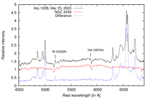
Figure 1: The spectra of Arp 102B (top) and NGC 4339 (75% flux of Arp 102B, middle) taken on Mar 25, 2003, and their difference (bottom) giving the AGN-continuum of Arp 102B.

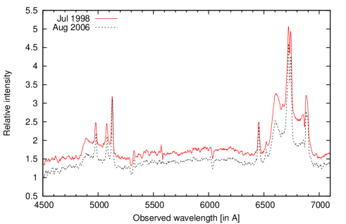
Figure 2: Two examples of the total optical spectrum of Arp 102B, when the object was in a high activity state in July 1998 (solid line), and when it was in a low activity state in Aug 2006 (dashed line).

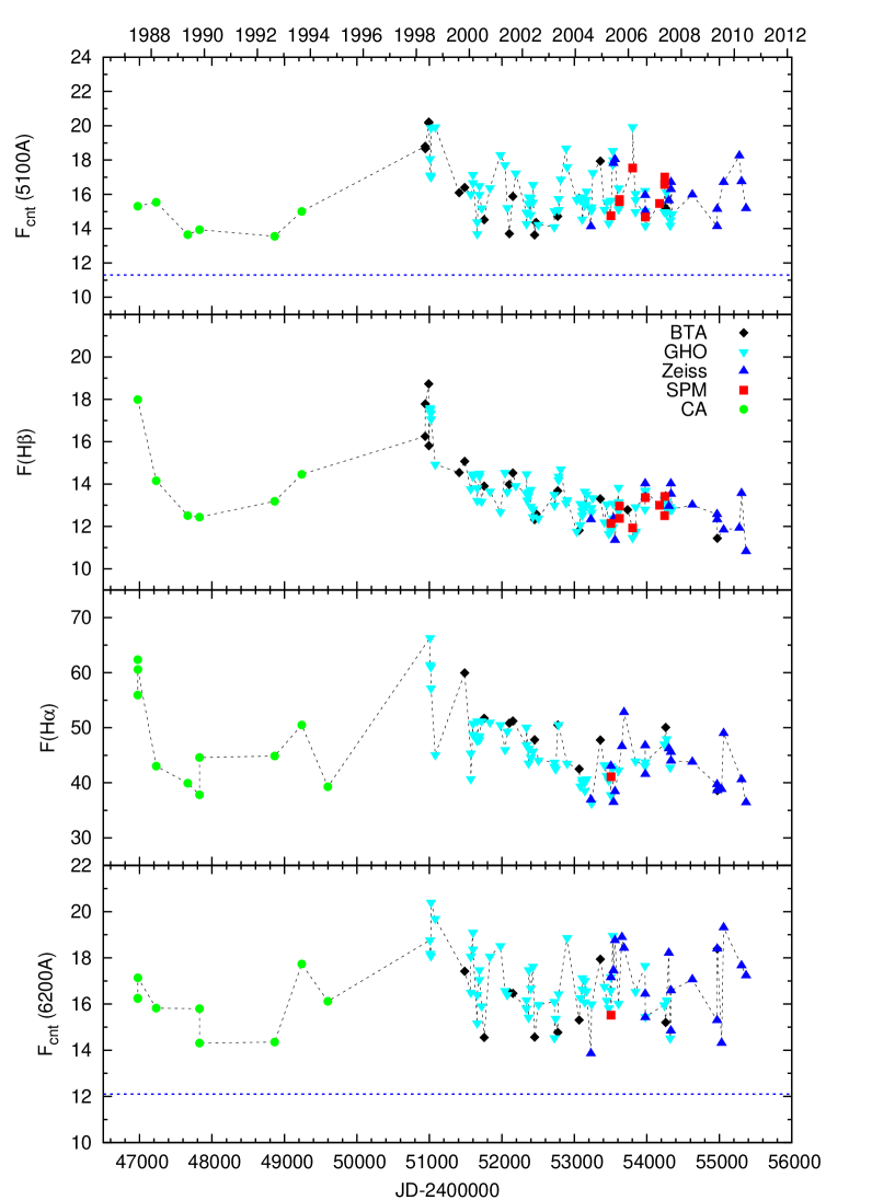
Figure 3: Light curves (from top to bottom) for the blue continuum flux, H$\beta$ and H$\alpha$ line flux, and red continuum flux. Observations with different telescopes are denoted with different symbols given in the middle plot. The continuum flux is in units 10^-16 erg cm⁻²s⁻¹A⁻¹, and the line flux in 10^-14 erg cm⁻²s⁻¹. The dashed line in the blue and red continuum light curves mark the contribution of the starlight-continuum of the host galaxy.

Table 1: Sources of spectroscopic observations.

Observatory	Code	Tel.aperture + equipment	Aperture	Focus
$\,\,\,\,\,\,\,\,\,\,\,\,1$	2	3	4	5
SAO(Russia)	L(N)	6 m + Long slit	2.0$\times$6.0	Nasmith
SAO(Russia)	L(U)	6 m + UAGS	2.0$\times$6.0	Prime
SAO(Russia)	L(Sc)	6 m + Scorpio	1.0$\times$6.07	Prime
Gullermo Haro (México)	GHO	2.1 m + B&C	2.5$\times$6.0	Cassegrain
San Pedro Martir (México)	SPM	2.1 m + B&C	2.5$\times$6.0	Cassegrain
SAO(Russia)	Z2K	1 m + GAD	4.0$\times$9.45	Cassegrain
Calar Alto(Spain)	CA1	3.5 m + B&C / TWIN	(1.5–2.1)$\times$3.5	Cassegrain
Calar Alto(Spain)	CA2	2.2 m + B&C	2.0$\times$3.5	Cassegrain

2

Table 2: The log of spectroscopic observations.

N	UT-date	JD	CODE	Aperture	Sp.range	Seeing
		2400000+		[arcsec]	[${\rm\AA}$]	[arcsec]
1	2	3	4	5	6	7
1	1987Jun28	46975.00	CA1	2.0x3.5	3690-7080	1.5 - 2.5
2	1987Jun29	46976.00	CA1	1.5x3.5	6360-7245	1.5 - 2.5
3	1987Jun30	46977.00	CA1	1.5x3.5	6360-7245	1.5 - 2.5
4	1988Mar08	47229.00	CA1	1.6x3.5	3720-7105	1.5 - 2.5
5	1989May18	47665.00	CA1	2.1x3.5	H$\beta$, H$\alpha$	1.5 - 2.5
6	1989Oct27	47827.00	CA1	2.0x3.5	4094-7440	1.5 - 2.5
7	1989Oct28	47828.00	CA1	2.0x3.5	4094-7440	1.5 - 2.5
8	1992Aug30	48865.00	CA2	2.0x3.5	3850-9100	1.5 - 2.5
9	1993Sep07	49238.00	CA1	2.1x3.5	3630-8310	1.5 - 2.5
10	1994Sep02	49598.00	CA2	2.0x3.5	4540-8520	1.5 - 2.5
11	1998May06	50940.34	L(N)	2.0x6.0	3700-6200	3.0
12	1998May08	50942.33	L(N)	2.0x6.0	3700-6200	2.0
13	1998Jun25	50990.29	L(N)	2.0x6.0	3600-6100	3.0
14	1998Jun26	50991.20	L(N)	2.0x6.0	3600-6100	3.0
15	1998Jul13	51008.30	GHO	2.5x6.0	3970-7224	2.1
16	1998Jul16	51011.23	GHO	2.5x6.0	4209-7479	2.8
17	1998Jul25	51020.26	GHO	2.5x6.0	3964-7235	2.5
18	1998Jul26	51021.27	GHO	2.5x6.0	3927-7222	2.1
19	1998Sep23	51079.50	GHO	2.5x6.0	4240-7538	2.5
20	1999Aug19	51410.30	L(U)	2.0x6.0	4500-5736	2.0
21	1999Nov03	51486.14	L(U)	2.0x6.0	3600-8350	1.3
22	2000Jan26	51569.97	GHO	2.5x6.0	4100-7400	2.7
23	2000Jan27	51570.96	GHO	2.5x6.0	4100-7400	1.8
24	2000Feb25	51599.92	GHO	2.5x6.0	4550-7850	3.0
25	2000Feb26	51600.88	GHO	2.5x6.0	4300-7600	3.0
26	2000Apr24	51658.87	GHO	2.5x6.0	4200-7500	3.0
27	2000Apr25	51659.83	GHO	2.5x6.0	4200-7500	3.0
28	2000May24	51689.47	GHO	2.5x6.0	4200-7500	2.5
29	2000May25	51689.54	GHO	2.5x6.0	4200-7500	2.5
30	2000Jun24	51719.74	GHO	2.5x6.0	4691-7991	3.0
31	2000Jul30	51756.26	L(U)	2.0x6.0	3670-6310	1.6
32	2000Oct17	51834.58	GHO	2.5x6.0	4000-7300	2.7
33	2001Mar12	51980.61	GHO	2.5x6.0	4200-7500	3.0
34	2001May11	52041.88	GHO	2.5x6.0	3600-6900	3.2
35	2001May13	52043.94	GHO	2.5x6.0	4100-7400	3.0
36	2001Jun13	52073.80	GHO	2.5x6.0	4100-7400	4.1
37	2001Jul10	52101.46	L(U)	2.0x6.0	5700-8124	2.0
38	2001Jul11	52102.48	L(U)	2.0x6.0	3600-6024	1.2
39	2001Aug29	52151.30	L(U)	2.0x6.0	3680-6104	2.5
40	2001Oct08	52190.62	GHO	2.5x6.0	3600-6900	2.7
41	2002Mar04	52337.91	GHO	2.5x6.0	3800-7100	2.0
42	2002Mar05	52338.91	GHO	2.5x6.0	5700-7460	2.0
43	2002Mar06	52339.97	GHO	2.5x6.0	4300-5900	2.0
44	2002Mar16	52349.94	GHO	2.5x6.0	4300-5900	2.0
45	2002Apr02	52366.85	GHO	2.5x6.0	4300-5900	1.8
46	2002Apr03	52367.83	GHO	2.5x6.0	5700-7460	1.5
47	2002Apr05	52369.88	GHO	2.5x6.0	3800-7100	1.5
48	2002May02	52396.82	GHO	2.5x6.0	4200-5960	2.3
49	2002May03	52397.76	GHO	2.5x6.0	5700-7460	2.0
50	2002May04	52398.77	GHO	2.5x6.0	4300-5900	2.0
51	2002Jun01	52426.82	GHO	2.5x6.0	4200-5850	2.7
52	2002Jun02	52427.78	GHO	2.5x6.0	5700-7460	3.2
53	2002Jun04	52429.77	GHO	2.5x6.0	4200-5960	3.2
54	2002Jun24	52450.37	L(U)	2.0x6.0	3430-5854	5.0
55	2002Jul15	52471.42	L(U)	2.0x6.0	3470-5894	2.0
56	2002Aug15	52501.65	GHO	2.5x6.0	4200-5700	2.3
57	2002Aug17	52503.68	GHO	2.5x6.0	5700-7460	2.0
58	2003Mar24	52722.93	GHO	2.5x6.0	4200-5850	2.7
59	2003Mar25	52723.92	GHO	2.5x6.0	3800-7100	2.7
60	2003Mar26	52724.96	GHO	2.5x6.0	5600-7462	2.3
61	2003Apr11	52740.86	GHO	2.5x6.0	5600-7462	3.6
62	2003May09	52769.26	L(U)	2.0x6.0	3650-6070	1.5
63	2003May11	52771.41	L(U)	2.0x6.0	5730-8151	1.5
64	2003May22	52781.79	GHO	2.5x6.0	3700-7430	3.6
65	2003May23	52782.87	GHO	2.5x6.0	4200-6085	2.3
66	2003Jun21	52811.85	GHO	2.5x6.0	4200-5960	2.3
67	2003Sep03	52885.65	GHO	2.5x6.0	4300-5900	4.1
68	2003Sep17	52899.69	GHO	2.5x6.0	3800-7100	2.3
69	2004Jan27	53032.00	GHO	2.5x6.0	4300-6060	2.5
70	2004Mar02	53066.59	L(U)	2.0x6.0	3700-6124	2.0
71	2004Mar16	53080.94	GHO	2.5x6.0	4300-6060	5.0
72	2004Mar18	53082.94	GHO	2.5x6.0	3800-7100	5.0
73	2004Apr11	53106.94	GHO	2.5x6.0	3800-7100	3.5
74	2004Apr12	53107.84	GHO	2.5x6.0	4300-6060	2.5
75	2004Apr13	53108.92	GHO	2.5x6.0	5700-7460	2.5
76	2004May18	53143.83	GHO	2.5x6.0	3800-7100	2.3
77	2004May19	53144.82	GHO	2.5x6.0	4300-6060	2.3
78	2004May20	53145.78	GHO	2.5x6.0	5700-7460	2.7
79	2004Jun10	53166.80	GHO	2.5x6.0	3800-7100	1.8
80	2004Jun11	53167.77	GHO	2.5x6.0	4300-6060	1.8
81	2004Aug10	53228.32	Z2K	4.0x9.45	3700-7450	2.0
82	2004Aug18	53235.64	GHO	2.5x6.0	4300-6060	3.1
83	2004Aug20	53237.63	GHO	2.5x6.0	3800-7100	2.7
84	2004Sep06	53254.63	GHO	2.5x6.0	4300-6060	2.7
85	2004Dec18	53357.50	L(Sc)	1.0x6.07	3460-7460	1.6
86	2005Feb13	53415.01	GHO	2.5x6.0	3830-7090	3.5
87	2005Mar17	53446.89	GHO	2.5x6.0	3700-7070	3.0
88	2005Apr15	53475.90	GHO	2.5x6.0	4240-5940	2.2
89	2005Apr16	53476.79	GHO	2.5x6.0	5220-7250	1.8
90	2005May11	53501.85	GHO	2.5x6.0	3750-7100	3.1
91	2005May12	53502.83	GHO	2.5x6.0	4220-5920	3.0
92	2005May12	53503.48	Z2K	4.0x9.45	3700-7450	2.0
93	2005May13	53503.83	GHO	2.5x6.0	5580-7300	2.2
94	2005May14	53504.73	SPM	2.5x6.0	3880-5970	4.8
95	2005May15	53505.85	SPM	2.5x6.0	5730-7810	3.3
96	2005Jun08	53529.85	GHO	2.5x6.0	3720-7070	1.9
97	2005Jun09	53530.64	GHO	2.5x6.0	4300-5960	3.0
98	2005Jun11	53532.78	GHO	2.5x6.0	4250-5940	3.5
99	2005Jun16	53538.46	Z2K	4.0x9.45	3700-7450	2.5
100	2005Jul07	53559.44	Z2K	4.0x9.45	3700-7450	5.0
101	2005Aug26	53608.70	GHO	2.5x6.0	3790-7100	2.6
102	2005Aug28	53610.64	GHO	2.5x6.0	4330-6000	2.8
103	2005Aug29	53611.63	GHO	2.5x6.0	4320-6000	3.5
104	2005Aug31	53613.62	GHO	2.5x6.0	4330-6000	2.7
105	2005Sep08	53621.67	SPM	2.5x6.0	3740-5770	3.0
106	2005Sep09	53622.67	SPM	2.5x6.0	3670-5800	2.8
107	2005Oct11	53655.23	Z2K	4.0x9.45	3700-7450	3-4
108	2005Nov09	53684.19	Z2K	4.0x9.45	3700-7450	2.7
109	2005Dec28	53732.50	L(Sc)	1.0x6.00	3100-7300	1.8
110	2006Mar08	53802.96	SPM	2.5x6.0	3740-5800	3.5
111	2006Mar08	53802.97	GHO	2.5x6.0	3740-7100	3.5
112	2006Apr17	53842.94	GHO	2.5x6.0	3720-7090	3.2
113	2006Apr18	53843.93	GHO	2.5x6.0	4240-5940	2.4
114	2006Apr19	53844.86	GHO	2.5x6.0	4240-5940	2.0
115	2006Aug28	53975.65	GHO	2.5x6.0	3600-7090	2.1
116	2006Aug28	53976.69	SPM	2.5x6.0	3720-5790	3.0
117	2006Aug29	53977.50	Z2K	4.0x9.45	3750-7390	5.0
118	2006Aug30	53977.63	GHO	2.5x6.0	4130-5920	2.5
119	2006Aug30	53978.48	Z2K	4.0x9.45	3700-7450	2.0
120	2006Aug31	53978.63	GHO	2.5x6.0	3530-7110	2.1
121	2007Mar15	54174.95	SPM	2.5x6.0	3740-5810	2.4
122	2007May20	54240.85	GHO	2.5x6.0	3780-7370	2.0
123	2007May23	54243.82	SPM	2.5x6.0	3730-5800	3.2
124	2007May26	54246.87	SPM	2.5x6.0	3750-5820	3.5
125	2007Jun08	54259.40	L(Sc)	1.0x6.07	3100-7300	2.3
126	2007Jun20	54271.76	GHO	2.5x6.0	4300-6120	3.0
127	2007Jun21	54272.85	GHO	2.5x6.0	3890-7480	2.1
128	2007Jul20	54302.38	Z2K	4.0x9.45	3700-7450	3.0
129	2007Aug10	54322.66	GHO	2.5x6.0	3880-7470	3.0
130	2007Aug11	54323.63	GHO	2.5x6.0	4350-6170	3.5
131	2007Aug18	54331.31	Z2K	4.0x9.45	3700-7450	3.0
132	2007Aug19	54332.33	Z2K	4.0x9.45	3700-7450	2.0
133	2007Sep04	54347.63	GHO	2.5x6.0	4150-5970	2.5
134	2008Jun08	54626.46	Z2K	4.0x9.45	3700-7450	2.5
135	2009May17	54969.47	Z2K	4.0x9.45	3700-7450	2.5
136	2009May19	54970.54	Z2K	4.0x9.45	3700-7450	3.0
137	2009May20	54972.20	L(Sc)	1.0x6.07	3100-7300	2.0
138	2009Jul17	55030.33	Z2K	4.0x9.45	3700-7450	2.5
139	2009Aug14	55058.38	Z2K	4.0x9.45	3700-7450	2.5
140	2010Mar21	55276.51	Z2K	4.0x9.45	3700-7450	2.6
141	2010Apr20	55306.52	Z2K	4.0x9.45	3700-7450	2.5
142	2010Jun19	55367.42	Z2K	4.0x9.45	3700-7450	2.5

Table 2: Continued.

2.2 Absolute calibration (scaling) of the spectra and measurements of spectra

The standard technique of the flux calibration of spectra (i.e. comparison with stars of known spectral energy distribution) is not precise enough for the study of the AGN variability, since even under good photometric conditions, the accuracy of spectrophotometry is usually not better than 10%. Therefore we used standard stars only to provide a relative flux calibration. For the absolute calibration, the fluxes of the narrow emission lines are adopted as a scaling factor of observed AGN spectra, since they are known to remain constant on time scales of tens of years (Peterson, 1993).

The scaling of the blue spectra was performed using the method of van Groningen & Wanders (1992) modified by Shapovalova et al. (2004). We will not repeat the scaling procedure here. This method allowed us to obtain a homogeneous set of spectra with the same wavelength calibration and the same [O III]$\lambda$4959+5007 flux. Blue spectra were scaled using [O III]$\lambda$4959+5007. Red spectra with a resolution of 8–10 Å do not contain these [O III] lines, but as a rule there was the blue spectra (R$\sim$8-10 Å or $\sim$15 Å) taken in the same night. Usually, the red edge of the blue spectra and the blue edge of the red spectra overlap in an interval of 300 Å. Therefore, first the red spectra were rescaled using the overlapping continuum region with the blue ones. Then, the blue spectrum was scaled with the [O III]$\lambda$4959+5007 line. In these cases, the scaling uncertainty was about 10%. Then scaling of the red spectrum was refined using the mean flux in [O I]$\lambda$6300 determined from a low-dispersion spectrum (R$\sim$12–15 Å). In Arp 102B we do not have data for [O III]$\lambda$5007+4959 in absolute units. Therefore we used the [O I]$\lambda$6300 in absolute units from Sergeev et al. (2000) F(6300)abs=(1.76$\pm$0.18)$\times$10^-14 erg cm^-2s^-1) and have calculated flux for [O III] lines to be F[O III]4959+5007=(4.9$\pm$0.49)$\times$10^-14 erg cm^-2s^-1. For this we used the good spectra of Arp 102B, containing both, the H$\alpha$ and H$\beta$ spectral bands (R$\sim$12-15 Å/px).

From the scaled spectra we determined the average flux in the blue continuum at the observed wavelength $\sim 5225$Å  (or at $\sim 5100$ Å  in the rest frame of Arp 102B, z=0.0241), by means of the flux averaging in the bandpass of 5200–5250 Å and in the red continuum the observed wavelength is $\sim 6381$ Å  (or at $\sim 6230$ Å  in the rest frame), averaging the flux in the wavelength range from 6356 Å to 6406 Å. In the above wavelength intervals there are no strong absorption lines from the host galaxy. For the determination of the observed fluxes of H$\beta$ and H$\alpha$, it is necessary to subtract the continuum contribution. For the continuum subtraction, a linear continuum was constructed using windows of 20 Å  width, located at 4700 Å  and 5240 Å  for the H$\beta$ spectral band, and at 6380 Å  and 7000 Å  for the H$\alpha$ one. After the continuum subtraction, we defined the observed fluxes in the lines in the following wavelength intervals: (4845-5150) Å  for H$\beta$, and (6500-6965) Å  for H$\alpha$ (the interval is like the one in Sergeev et al., 2000).

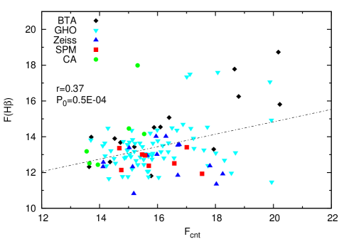
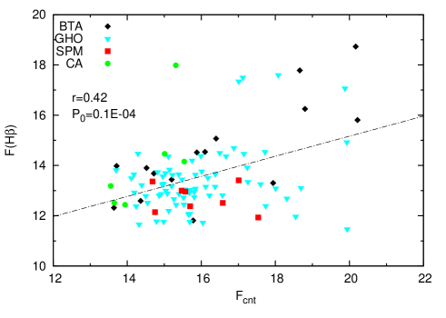
Figure 4: H$\beta$ vs continuum flux. Upper plot: all observed data. Bottom: without data observed with the Zeiss telescope. The continuum flux is in units $10^{-16}\rm erg\ cm^{-2}s^{-1}A^{-1}$, and the line flux in $10^{-14}\rm erg\ cm^{-2}s^{-1}$. Observations with different telescopes are denoted with different symbols given in the upper left. The correlation coefficient and the corresponding p-value are also given.

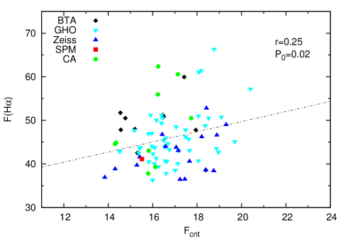
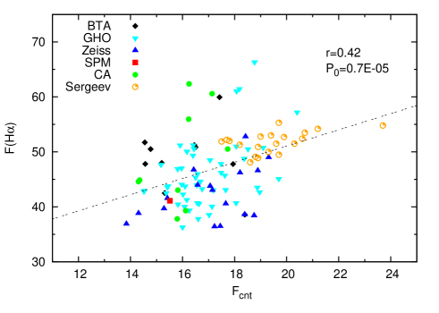
Figure 5: The same as Fig. 4 but for H$\alpha$ (upper) The bottom panel includes also data from Sergeev et al. (2000).

Table 3: Flux scale factors for optical spectra.

Sample	Years	Aperture	Scale factor	Extended source correction
		(arcsec)	($\varphi$)	G(g)
L(U,N)	1998–2004	2.0$\times$6.0	1.000	0.000
L(Sc)	2004–2009	1.0$\times$6.0	1.019	-0.391
GHO,SPM	1998–2007	2.5$\times$6.0	1.000	0.000
Z2K	2004–2005	4.0$\times$9.45	1.027	0.304
Z2K	2006–2010	4.0$\times$9.45	1.027	0.633
CA1	1987–1993	1.5–2.1$\times$3.5	$\sim$ 1	-0.200–0.000
CA2	1992–1994	2.0$\times$3.5	$\sim$ 1	0.000
In units 10${}^{-15}\rm ergs^{-1}cm^{-2}\AA^{-1}$

4

Table 4: The measured continuum and line fluxes.

N	UT-date	MJD	F${}_{\rm blue\ cnt}\pm\sigma$	F${}_{\rm blue\ cnt}^{\rm corr}\pm\sigma$	F(H$\beta$)$\pm\sigma$	F(H$\alpha$)$\pm\sigma$	F${}_{\rm red\ cnt}\pm\sigma$	F${}_{\rm red\ cnt}^{\rm corr}\pm\sigma$
1	2	3	4	5	6	7	8	9
1	1987Jun28	46975.00	15.31	4.01	17.99$\pm$1.01	62.38$\pm$3.49	16.25$\pm$0.50	4.15$\pm$0.37
2	1987Jun29	46976.00	-	-	-	55.95$\pm$3.13	16.24$\pm$0.50	4.14$\pm$0.37
3	1987Jun30	46977.00	-	-	-	60.58$\pm$3.39	17.13$\pm$0.53	5.03$\pm$0.45
4	1988Mar08	47229.00	15.54$\pm$0.96	4.24$\pm$0.40	14.16$\pm$0.99	43.04$\pm$4.35	15.82$\pm$1.42	3.72$\pm$0.33
5	1989May18	47665.00	13.65$\pm$0.85	2.35$\pm$0.22	12.51$\pm$0.88	39.93$\pm$4.03	-
6	1989Oct27	47827.00	-	-	-	37.82$\pm$3.82	15.80$\pm$1.42	3.70$\pm$0.33
7	1989Oct28	47828.00	13.94$\pm$0.86	2.64$\pm$0.25	12.44$\pm$0.87	44.60$\pm$4.50	14.31$\pm$1.29	2.21$\pm$0.20
8	1992Aug30	48865.00	13.55$\pm$0.84	2.25$\pm$0.21	13.18$\pm$0.92	44.88$\pm$4.53	14.35$\pm$1.29	2.25$\pm$0.20
9	1993Sep07	49238.00	15.01$\pm$0.93	3.71$\pm$0.35	14.46$\pm$1.01	50.52$\pm$5.10	17.73$\pm$1.60	5.63$\pm$0.50
10	1994Sep02	49598.00	-	-	-	39.30$\pm$3.97	16.12$\pm$1.45	4.02$\pm$0.36
11	1998May06	50940.34	18.80$\pm$ 0.64	7.50$\pm$0.71	16.25$\pm$ 0.49	-	-
12	1998May08	50942.33	18.66$\pm$ 0.63	7.36$\pm$0.70	17.78$\pm$ 0.53	-	-
13	1998Jun25	50990.29	20.17$\pm$ 0.69	8.87$\pm$0.84	18.73$\pm$ 2.25	-	-
14	1998Jun26	50991.20	20.22$\pm$ 0.69	8.92$\pm$0.85	15.81$\pm$ 1.90	-	-
15	1998Jul13	51008.30	18.08$\pm$ 0.61	6.78$\pm$0.64	17.60$\pm$ 0.53	66.33$\pm$2.72	18.77$\pm$ 0.83	6.67$\pm$0.59
16	1998Jul16	51011.23	17.12$\pm$ 0.58	5.82$\pm$0.55	17.50$\pm$ 0.53	61.46$\pm$2.52	18.19$\pm$ 0.80	6.09$\pm$0.54
17	1998Jul25	51020.26	17.01$\pm$ 1.87	5.71$\pm$0.54	17.35$\pm$ 0.52	61.06$\pm$2.50	18.08$\pm$ 1.54	5.98$\pm$0.53
18	1998Jul26	51021.27	19.88$\pm$ 2.19	8.58$\pm$0.82	17.07$\pm$ 0.51	57.22$\pm$2.35	20.40$\pm$ 1.73	8.30$\pm$0.74
19	1998Sep23	51079.50	19.93$\pm$ 0.68	8.63$\pm$0.82	14.93$\pm$ 0.45	45.11$\pm$1.85	19.70$\pm$ 0.87	7.60$\pm$0.68
20	1999Aug19	51410.30	16.10$\pm$ 0.55	4.80$\pm$0.46	14.54$\pm$ 0.44	-	-
21	1999Nov03	51486.14	16.40$\pm$ 0.56	5.10$\pm$0.48	15.07$\pm$ 0.45	59.96$\pm$2.46	17.42$\pm$ 0.77	5.32$\pm$0.47
22	2000Jan26	51569.97	16.01$\pm$ 0.54	4.71$\pm$0.45	13.77$\pm$ 0.41	45.36$\pm$3.45	16.50$\pm$ 0.73	4.40$\pm$0.39
23	2000Jan27	51570.96	-	-	-	40.73$\pm$3.10	18.06$\pm$ 0.79	5.96$\pm$0.53
24	2000Feb25	51599.92	16.67$\pm$ 0.57	5.37$\pm$0.51	14.37$\pm$ 0.43	50.77$\pm$2.08	19.10$\pm$ 0.84	7.00$\pm$0.62
25	2000Feb26	51600.88	17.15$\pm$ 0.58	5.85$\pm$0.56	14.47$\pm$ 0.43	48.77$\pm$2.00	18.37$\pm$ 0.81	6.27$\pm$0.56
26	2000Apr24	51658.87	13.70$\pm$ 0.47	2.40$\pm$0.23	13.82$\pm$ 0.41	47.69$\pm$1.96	15.17$\pm$ 0.67	3.07$\pm$0.27
27	2000Apr25	51659.83	14.39$\pm$ 0.49	3.09$\pm$0.29	13.22$\pm$ 0.40	51.24$\pm$2.10	16.41$\pm$ 0.72	4.31$\pm$0.38
28	2000May24	51689.47	16.50$\pm$ 0.56	5.20$\pm$0.49	14.50$\pm$ 0.44	47.83$\pm$1.96	17.48$\pm$ 0.77	5.38$\pm$0.48
29	2000May25	51689.54	15.99$\pm$ 0.54	4.69$\pm$0.45	14.38$\pm$ 0.43	48.52$\pm$1.99	17.06$\pm$ 0.75	4.96$\pm$0.44
30	2000Jun24	51719.74	15.20$\pm$ 0.52	3.90$\pm$0.37	13.18$\pm$ 0.40	51.22$\pm$2.10	15.91$\pm$ 0.70	3.81$\pm$0.34
31	2000Jul30	51756.26	14.52$\pm$ 0.49	3.22$\pm$0.31	13.90$\pm$ 0.42	51.73$\pm$2.12	14.55$\pm$ 0.64	2.45$\pm$0.22
32	2000Oct17	51834.58	16.38$\pm$ 0.56	5.08$\pm$0.48	13.66$\pm$ 0.41	51.01$\pm$2.09	18.06$\pm$ 0.79	5.96$\pm$0.53
33	2001Mar12	51980.61	18.31$\pm$ 0.62	7.01$\pm$0.67	12.69$\pm$ 0.38	50.53$\pm$2.07	18.52$\pm$ 0.81	6.42$\pm$0.57
34	2001May11	52041.88	17.72$\pm$ 0.60	6.42$\pm$0.61	14.54$\pm$ 0.44	-	-
35	2001May13	52043.94	-	-	-	46.01$\pm$1.89	16.58$\pm$ 0.73	4.48$\pm$0.40
36	2001Jun13	52073.80	15.22$\pm$ 0.52	3.92$\pm$0.37	13.63$\pm$ 0.41	49.35$\pm$2.02	16.40$\pm$ 0.72	4.30$\pm$0.38
37	2001Jul10	52101.46	-	-	-	50.84$\pm$2.08	16.50$\pm$ 0.73	4.40$\pm$0.39
38	2001Jul11	52102.48	13.71$\pm$ 0.47	2.41$\pm$0.23	13.98$\pm$ 0.42	-	-
39	2001Aug29	52151.30	15.88$\pm$ 0.54	4.58$\pm$0.44	14.52$\pm$ 0.44	51.24$\pm$2.10	16.46$\pm$ 0.72	4.36$\pm$0.39
40	2001Oct08	52190.62	17.24$\pm$ 0.59	5.94$\pm$0.56	13.92$\pm$ 0.42	-	-
41	2002Mar04	52337.91	14.96$\pm$ 0.51	3.66$\pm$0.35	13.57$\pm$ 0.41	46.92$\pm$1.92	15.81$\pm$ 0.70	3.71$\pm$0.33
42	2002Mar05	52338.91	-	-	-	50.09$\pm$2.05	16.18$\pm$ 0.71	4.08$\pm$0.36
43	2002Mar06	52339.97	14.29$\pm$ 0.49	2.99$\pm$0.28	14.48$\pm$ 0.43	-	-
44	2002Mar16	52349.94	14.95$\pm$ 0.51	3.65$\pm$0.35	13.24$\pm$ 0.40	-	-
45	2002Apr02	52366.85	15.48$\pm$ 0.53	4.18$\pm$0.40	13.45$\pm$ 0.40	-	-
46	2002Apr03	52367.83	-	-	-	43.56$\pm$1.79	15.42$\pm$ 1.37	3.32$\pm$0.30
47	2002Apr05	52369.88	15.84$\pm$ 0.54	4.54$\pm$0.43	13.64$\pm$ 0.41	46.24$\pm$1.90	17.48$\pm$ 1.56	5.38$\pm$0.48
48	2002May02	52396.82	14.82$\pm$ 0.50	3.52$\pm$0.33	13.74$\pm$ 0.41	-	-
49	2002May03	52397.76	-	-	-	44.64$\pm$1.83	16.68$\pm$ 0.73	4.58$\pm$0.41
50	2002May04	52398.77	15.81$\pm$ 0.54	4.51$\pm$0.43	12.95$\pm$ 0.39	-	-
51	2002Jun01	52426.82	15.53$\pm$ 0.53	4.23$\pm$0.40	12.45$\pm$ 0.37	-	-
52	2002Jun02	52427.78	-	-	-	45.72$\pm$1.87	17.63$\pm$ 0.78	5.53$\pm$0.49
53	2002Jun04	52429.77	16.57$\pm$ 0.56	5.27$\pm$0.50	12.82$\pm$ 0.38	-	-
54	2002Jun24	52450.37	13.64$\pm$ 0.46	2.34$\pm$0.22	12.32$\pm$ 0.37	47.82$\pm$1.96	14.57$\pm$ 0.64	2.47$\pm$0.22
55	2002Jul15	52471.42	14.36$\pm$ 0.49	3.06$\pm$0.29	12.59$\pm$ 0.38	-	-
56	2002Aug15	52501.65	14.24$\pm$ 0.48	2.94$\pm$0.28	12.38$\pm$ 0.37	-	-
57	2002Aug17	52503.68	-	-	-	44.08$\pm$1.81	15.97$\pm$ 0.70	3.87$\pm$0.34
58	2003Mar24	52722.93	14.11$\pm$ 0.48	2.81$\pm$0.27	13.50$\pm$ 0.41	-	-
59	2003Mar25	52723.92	15.04$\pm$ 0.51	3.74$\pm$0.36	13.00$\pm$ 0.39	43.74$\pm$1.79	16.10$\pm$ 1.18	4.00$\pm$0.36
60	2003Mar26	52724.96	-	-	-	42.96$\pm$1.76	14.53$\pm$ 1.06	2.43$\pm$0.22
61	2003Apr11	52740.86	-	-	-	42.51$\pm$1.74	15.37$\pm$ 0.68	3.27$\pm$0.29
62	2003May09	52769.26	14.72$\pm$ 0.50	3.42$\pm$0.32	13.68$\pm$ 0.41	-	-
63	2003May11	52771.41	-	-	-	50.50$\pm$1.80	14.77$\pm$ 0.65	2.67$\pm$0.24
64	2003May22	52781.79	15.75$\pm$ 0.54	4.45$\pm$0.42	14.20$\pm$ 0.43	50.55$\pm$2.07	16.44$\pm$ 0.72	4.34$\pm$0.39
65	2003May23	52782.87	15.11$\pm$ 0.51	3.81$\pm$0.36	14.36$\pm$ 0.43	-	-
66	2003Jun21	52811.85	16.88$\pm$ 0.57	5.58$\pm$0.53	14.70$\pm$ 0.44	-	-
67	2003Sep03	52885.65	18.69$\pm$ 0.64	7.39$\pm$0.70	13.11$\pm$ 0.39	-	-
68	2003Sep17	52899.69	17.60$\pm$ 0.60	6.30$\pm$0.60	13.26$\pm$ 0.40	43.53$\pm$1.78	18.87$\pm$ 0.83	6.77$\pm$0.60
69	2004Jan27	53032.00	15.69$\pm$ 0.53	4.39$\pm$0.42	11.76$\pm$ 0.35	-	-
70	2004Mar02	53066.59	15.78$\pm$ 0.54	4.48$\pm$0.43	11.81$\pm$ 0.35	42.52$\pm$1.74	15.31$\pm$ 0.67	3.21$\pm$0.29
71	2004Mar16	53080.94	15.69$\pm$ 0.53	4.39$\pm$0.42	12.08$\pm$ 0.36	-	-
72	2004Mar18	53082.94	15.84$\pm$ 0.54	4.54$\pm$0.43	13.08$\pm$ 0.39	39.38$\pm$1.61	16.27$\pm$ 0.72	4.17$\pm$0.37
73	2004Apr11	53106.94	15.81$\pm$ 0.54	4.51$\pm$0.43	12.75$\pm$ 0.38	40.61$\pm$1.67	16.64$\pm$ 0.73	4.54$\pm$0.40
74	2004Apr12	53107.84	14.55$\pm$ 0.49	3.25$\pm$0.31	12.52$\pm$ 0.38	-	-
75	2004Apr13	53108.92	-	-	-	40.09$\pm$1.64	17.13$\pm$ 0.75	5.03$\pm$0.45
76	2004May18	53143.83	15.39$\pm$ 0.52	4.09$\pm$0.39	13.65$\pm$ 0.41	40.05$\pm$1.64	16.08$\pm$ 0.71	3.98$\pm$0.35
77	2004May19	53144.82	15.40$\pm$ 0.52	4.10$\pm$0.39	12.87$\pm$ 0.39	-	-
78	2004May20	53145.78	-	-	-	38.57$\pm$1.58	17.02$\pm$ 0.75	4.92$\pm$0.44
79	2004Jun10	53166.80	16.18$\pm$ 0.55	4.88$\pm$0.46	13.51$\pm$ 0.41	40.71$\pm$1.67	16.57$\pm$ 0.73	4.47$\pm$0.40
80	2004Jun11	53167.77	15.70$\pm$ 0.53	4.40$\pm$0.42	13.03$\pm$ 0.39	-	-
81	2004Aug10	53228.32	14.12$\pm$ 0.48	2.82$\pm$0.27	12.32$\pm$ 0.37	36.90$\pm$1.51	13.85$\pm$ 0.61	1.75$\pm$0.16
82	2004Aug18	53235.64	15.08$\pm$ 0.51	3.78$\pm$0.36	12.89$\pm$ 0.39	-	-
83	2004Aug20	53237.63	15.26$\pm$ 0.52	3.96$\pm$0.38	12.67$\pm$ 0.38	36.29$\pm$1.49	16.00$\pm$ 0.70	3.90$\pm$0.35
84	2004Sep06	53254.63	17.26$\pm$ 0.59	5.96$\pm$0.57	13.35$\pm$ 0.40	-	-
85	2004Dec18	53357.50	17.94$\pm$ 0.61	6.64$\pm$0.63	13.30$\pm$ 0.40	47.78$\pm$1.96	17.94$\pm$ 0.79	5.84$\pm$0.52
86	2005Feb13	53415.01	15.12$\pm$ 0.51	3.82$\pm$0.36	12.20$\pm$ 0.37	43.26$\pm$1.77	16.76$\pm$ 0.74	4.66$\pm$0.42
87	2005Mar17	53446.89	15.55$\pm$ 0.53	4.25$\pm$0.40	13.05$\pm$ 0.39	41.30$\pm$1.69	16.16$\pm$ 0.71	4.06$\pm$0.36
88	2005Apr15	53475.90	14.32$\pm$ 0.49	3.02$\pm$0.29	11.66$\pm$ 0.35	-	-
89	2005Apr16	53476.79	-	-	-	40.47$\pm$1.66	15.83$\pm$ 0.70	3.73$\pm$0.33
90	2005May11	53501.85	15.65$\pm$ 0.53	4.35$\pm$0.41	12.07$\pm$ 0.36	43.06$\pm$1.77	17.18$\pm$ 0.76	5.08$\pm$0.45
91	2005May12	53502.83	14.79$\pm$ 0.50	3.49$\pm$0.33	11.78$\pm$ 0.35	-	-
92	2005May12	53503.48	-	-	-	43.04$\pm$1.76	17.15$\pm$ 0.75	5.05$\pm$0.45
93	2005May13	53503.83	-	-	-	37.84$\pm$1.55	16.60$\pm$ 0.73	4.50$\pm$0.40
94	2005May14	53504.73	14.75$\pm$ 0.50	3.45$\pm$0.33	12.14$\pm$ 0.36	-	-
95	2005May15	53505.85	-	-	-	41.10$\pm$1.69	15.52$\pm$ 0.68	3.42$\pm$0.30
96	2005Jun08	53529.85	18.55$\pm$ 0.63	7.25$\pm$0.69	11.97$\pm$ 0.36	42.69$\pm$1.75	18.96$\pm$ 0.83	6.86$\pm$0.61
97	2005Jun09	53530.64	17.74$\pm$ 0.60	6.44$\pm$0.61	12.39$\pm$ 0.37	-	-
98	2005Jun11	53532.78	18.01$\pm$ 0.61	6.71$\pm$0.64	13.09$\pm$ 0.39	-	-
99	2005Jun16	53538.46	17.81$\pm$ 0.61	6.51$\pm$0.62	12.37$\pm$ 0.37	36.47$\pm$1.50	17.45$\pm$ 0.77	5.35$\pm$0.48
100	2005Jul07	53559.44	18.03$\pm$ 0.61	6.73$\pm$0.64	11.35$\pm$ 0.34	38.42$\pm$1.58	18.75$\pm$ 0.83	6.65$\pm$0.59
101	2005Aug26	53608.70	15.14$\pm$ 0.51	3.84$\pm$0.36	13.84$\pm$ 0.42	42.30$\pm$1.73	16.02$\pm$ 0.70	3.92$\pm$0.35
102	2005Aug28	53610.64	16.37$\pm$ 0.56	5.07$\pm$0.48	13.16$\pm$ 0.39	-	-
103	2005Aug29	53611.63	15.52$\pm$ 0.53	4.22$\pm$0.40	12.73$\pm$ 0.38	-	-
104	2005Aug31	53613.62	15.32$\pm$ 0.52	4.02$\pm$0.38	12.44$\pm$ 0.37	-	-
105	2005Sep08	53621.67	15.70$\pm$ 0.53	4.40$\pm$0.42	12.38$\pm$ 0.37	-	-
106	2005Sep09	53622.67	15.57$\pm$ 0.53	4.27$\pm$0.41	12.96$\pm$ 0.39	-	-
107	2005Oct11	53655.23	-	-	-	46.61$\pm$1.91	18.89$\pm$ 0.83	6.79$\pm$0.60
108	2005Nov09	53684.19	-	-	-	52.79$\pm$2.16	18.42$\pm$ 0.81	6.32$\pm$0.56
109	2005Dec28	53732.50	-	-	12.79$\pm$ 0.38	48.46$\pm$1.99	-
110	2006Mar08	53802.96	17.54$\pm$ 0.60	6.24$\pm$0.59	11.93$\pm$ 0.36	-	-
111	2006Mar08	53802.97	19.94$\pm$ 0.68	8.64$\pm$0.82	11.47$\pm$ 0.34	-	-
112	2006Apr17	53842.94	14.98$\pm$ 0.51	3.68$\pm$0.35	11.77$\pm$ 0.35	43.97$\pm$1.80	16.54$\pm$ 0.73	4.44$\pm$0.40
113	2006Apr18	53843.93	16.04$\pm$ 0.55	4.74$\pm$0.45	11.73$\pm$ 0.35	-	-
114	2006Apr19	53844.86	15.68$\pm$ 0.53	4.38$\pm$0.42	12.92$\pm$ 0.39	-	-
115	2006Aug28	53975.65	16.22$\pm$ 0.55	4.92$\pm$0.47	12.81$\pm$ 0.38	43.11$\pm$1.77	17.66$\pm$ 0.78	5.56$\pm$0.50
116	2006Aug28	53976.69	14.68$\pm$ 0.50	3.38$\pm$0.32	13.36$\pm$ 0.40	-	-
117	2006Aug29	53977.50	15.95$\pm$ 0.54	4.65$\pm$0.44	14.02$\pm$ 0.42	46.75$\pm$1.92	16.43$\pm$ 0.72	4.33$\pm$0.39
118	2006Aug30	53977.63	15.03$\pm$ 0.51	3.73$\pm$0.35	13.70$\pm$ 0.41	-	-
119	2006Aug30	53978.48	15.02$\pm$ 0.51	3.72$\pm$0.35	13.38$\pm$ 0.40	41.55$\pm$1.70	15.42$\pm$ 0.68	3.32$\pm$0.30
120	2006Aug31	53978.63	14.18$\pm$ 0.48	2.88$\pm$0.27	13.65$\pm$ 0.41	43.79$\pm$1.80	15.45$\pm$ 0.68	3.35$\pm$0.30
121	2007Mar15	54174.95	15.47$\pm$ 0.53	4.17$\pm$0.40	13.00$\pm$ 0.39	-	-
122	2007May20	54240.85	14.98$\pm$ 1.08	3.68$\pm$0.35	13.28$\pm$ 0.40	47.04$\pm$1.93	15.96$\pm$ 0.70	3.86$\pm$0.34
123	2007May23	54243.82	16.58$\pm$ 1.19	5.28$\pm$0.50	12.51$\pm$ 0.38	-	-
124	2007May26	54246.87	17.01$\pm$ 0.58	5.71$\pm$0.54	13.41$\pm$ 0.40	-	-
125	2007Jun08	54259.40	15.20$\pm$ 0.52	3.90$\pm$0.37	13.44$\pm$ 0.40	50.07$\pm$2.05	15.20$\pm$ 0.67	3.10$\pm$0.28
126	2007Jun20	54271.76	16.12$\pm$ 0.55	4.82$\pm$0.46	13.16$\pm$ 0.39	-	-
127	2007Jun21	54272.85	14.91$\pm$ 0.51	3.61$\pm$0.34	12.87$\pm$ 0.39	47.99$\pm$1.97	16.17$\pm$ 0.71	4.07$\pm$0.36
128	2007Jul20	54302.38	15.64$\pm$ 0.53	4.34$\pm$0.41	12.95$\pm$ 0.39	46.22$\pm$1.90	18.21$\pm$ 0.80	6.11$\pm$0.54
129	2007Aug10	54322.66	14.19$\pm$ 0.48	2.89$\pm$0.27	12.93$\pm$ 0.39	42.82$\pm$1.76	14.52$\pm$ 0.64	2.42$\pm$0.22
130	2007Aug11	54323.63	14.50$\pm$ 0.49	3.20$\pm$0.30	12.79$\pm$ 0.38	-	-
131	2007Aug18	54331.31	16.29$\pm$ 0.55	4.99$\pm$0.47	14.02$\pm$ 0.42	45.58$\pm$1.87	14.84$\pm$ 0.65	2.74$\pm$0.24
132	2007Aug19	54332.33	16.70$\pm$ 0.57	5.40$\pm$0.51	13.52$\pm$ 0.41	43.98$\pm$1.80	16.58$\pm$ 0.73	4.48$\pm$0.40
133	2007Sep04	54347.63	14.86$\pm$ 0.51	3.56$\pm$0.34	12.81$\pm$ 0.38	-	-
134	2008Jun08	54626.46	15.98$\pm$ 0.54	4.68$\pm$0.44	13.01$\pm$ 0.39	43.78$\pm$1.79	17.06$\pm$ 0.75	4.96$\pm$0.44
135	2009May17	54969.47	14.13$\pm$ 0.48	2.83$\pm$0.27	12.57$\pm$ 0.38	39.68$\pm$1.63	15.29$\pm$ 1.57	3.19$\pm$0.28
136	2009May19	54970.54	15.14$\pm$ 0.51	3.84$\pm$0.36	12.32$\pm$ 0.37	38.61$\pm$1.58	18.39$\pm$ 1.89	6.29$\pm$0.56
137	2009May20	54972.20	-	-	11.44$\pm$ 0.34	38.59$\pm$1.58	18.39$\pm$ 1.89	6.29$\pm$0.56
138	2009Jul17	55030.33	-	-	-	38.83$\pm$1.59	14.31$\pm$ 0.63	2.21$\pm$0.20
139	2009Aug14	55058.38	16.70$\pm$ 0.57	5.40$\pm$0.51	11.84$\pm$ 0.36	49.00$\pm$2.01	19.31$\pm$ 0.85	7.21$\pm$0.64
140	2010Mar21	55276.51	18.25$\pm$ 0.62	6.95$\pm$0.66	11.92$\pm$ 0.36	-	-
141	2010Apr20	55306.52	16.75$\pm$ 0.57	5.45$\pm$0.52	13.56$\pm$ 0.41	40.59$\pm$1.66	17.66$\pm$ 0.78	5.56$\pm$0.50
142	2010Jun19	55367.42	15.18$\pm$ 0.52	3.88$\pm$0.37	10.82$\pm$ 0.32	36.41$\pm$1.49	17.23$\pm$ 0.76	5.13$\pm$0.46

Table 4: Continued.

Table 5: Estimates of the errors for line and line-segment fluxes.

Line	Spectral region		$\sigma\pm$e (host-galaxy corrected)	$V_{r}$ region
	[Å] (obs)	[Å] (rest)	[%]	[km s-1]
cont 5100	5200–5250	5077–5126	3.4$\pm$2.6 (9.5$\pm$6.2)	-
cont 6200	6356–6406	6206–6255	4.4$\pm$3.1 (8.9$\pm$6.0)	-
H$\alpha$ - total	6500–6965	6347–6801	4.1$\pm$2.8 (4.1$\pm$2.8)	(-9875;+10865)
H$\beta$ - total	4845–5150	4731–5028	3.0$\pm$2.3 (3.2$\pm$2.8)	(-8074;+10291)
H$\alpha$ - blue	6540–6660	6386–6503	3.7$\pm$2.8	(-8090; -2730)
H$\alpha$ - core	6660–6760	6503–6600	3.3$\pm$2.2	(-2730; +1741)
H$\alpha$ - red 1	6760–6860	6600–6698	4.5$\pm$2.2	(+1739; +6197)
H$\alpha$ - red 2	6920–6940	6757–6776	13.1$\pm$15.3	(+8875; +9768)
H$\beta$ - blue	4854–4937	4739–4820	5.8$\pm$4.2	(-7532; -2531)
H$\beta$ - core	4937–5021	4820–4902	4.3$\pm$3.6	(-2531; +2531)
H$\beta$ - red	5021–5104	4902–4984	4.3$\pm$3.2	(+2531; +7532)

2.3 Unification of the spectral data

In order to investigate the long term spectral variability of an AGN, it is necessary to make a consistent, uniformed data set. Since observations were carried out with four different instruments, one has to correct the line and continuum fluxes for aperture effects (Peterson & Collins, 1983). As in our previous papers (Shapovalova et al., 2001, 2004, 2008, 2010, 2012) we determined a point-source correction factor ($\varphi$) and correction for contribution host galaxy (G) using the the following expressions (see Peterson et al., 1995):

$$F({\rm H}\beta)_{\rm true}=\varphi\cdot F({\rm H}\beta)_{\rm obs},$$

where $F({\rm H}\beta)_{\rm obs}$ is the observed H$\beta$ flux; $F({\rm H}\beta)_{\rm true}$ is the aperture corrected H$\beta$ flux. And

$$F({\rm cnt})_{\rm true}=\varphi\cdot F({\rm cont})_{\rm obs}-G(g),$$

where $F({\rm cnt})_{\rm obs}$ is the continuum flux at observed wavelength; $G(g)$ is an aperture-dependent correction factor to account for the host galaxy contribution.

The GHO observing scheme (Table 1), which correspond to a projected aperture ($2.5\arcsec\times 6.0\arcsec$) of the 2.1 m telescope, was adopted as a standard with $\varphi=1.0$ and $G(g)=0.0$, since with the GHO we collected the largest number of observed spectra of Arp102B.

The correction factors $\varphi$ and $G(g)$ are determined empirically by comparing pairs of simultaneous observations from each of given telescope data sets to that of the standard data set (as it was done in AGN Watch (as e.g. Peterson et al., 1994, 1999, 2002). Due to the small number of CA spectra (1987–1994) it was impossible to determine the correction factors as described above. The CA apertures for 7 spectra were close to our standard (slit width $2.0\arcsec-2.1\arcsec$) so we set $\varphi$=1.000 and $G(g)$=0.000, while for only 3 spectra - JD2446976 (1987Jun29), JD2446977 (1987Jun30) and JD2447229 (1988Mar08) the slit width was different ($1.5\arcsec$). In these last cases we expect that the corrections are the average between the aperture $1.0\arcsec$ and $2.0\arcsec$ (Table 3). However, in any case, to CA fluxes should be taken with caution. In practice, intervals which we defined as ”nearly simultaneous” are typically of 1-3 days. Therefore, the variability on short time scales ($<$ 3 days) is suppressed. The point-source correction factors and $G(g)$ values for different samples are listed in Table 3. Using these factors, we re-calibrated the observed fluxes of H$\alpha$, H$\beta$, and the blue and red continuum to a common scale corresponding to our standard aperture $2.5\arcsec\times 6.0\arcsec$ (Table LABEL:tab4). Also we determined the observed fluxes in the H$\alpha,\beta$ line-segments (core and wings – the wavelengths intervals are given in Table 5). Then we re-calibrated the H$\alpha,\beta$ line-segment fluxes to a common scale that corresponds to our standard aperture $2.5\arcsec\times 6.0\arcsec$ (see Tables LABEL:tab_seg_ha-LABEL:tab_seg_hb). The mean errors (uncertainties) in the observed continuum fluxes and in the observed fluxes of emission lines and their segments are given in Table 5.

6

Table 6: The measured line segment fluxes of H$\alpha$ in units of $10^{-14}\rm erg\,cm^{-2}s^{-1}$.

N	MJD	F(H$\alpha$)blue	F(H$\alpha$)red1	F(H$\alpha$)red2	F(H$\alpha$)core
1	46975	14.794	11.854	0.887	24.248
2	46976	12.816	10.648	0.920	21.660
3	46977	14.383	11.946	0.933	23.243
4	47229	10.668	7.403	0.388	17.304
5	47827	8.576	6.254	0.557	15.528
6	47828	10.540	7.367	0.674	17.832
7	48865	9.416	7.215	0.804	18.006
8	49238	11.721	7.845	0.660	21.903
9	49598	7.755	7.066	0.611	16.159
10	51008	18.692	13.213	0.427	25.368
11	51011	16.101	12.064	0.509	24.633
12	51020	16.001	11.986	0.501	24.474
13	51021	15.167	11.007	0.480	23.163
14	51079	12.188	8.036	0.305	19.490
15	51486	15.873	12.697	0.511	26.352
16	51569	11.241	8.229	0.316	18.947
17	51570	10.084	7.563	0.265	17.343
18	51599	12.826	9.327	0.396	20.861
19	51600	12.494	8.875	0.424	19.998
20	51658	10.760	8.735	0.625	20.116
21	51659	11.664	9.490	0.608	21.453
22	51689	11.013	8.831	0.592	19.831
23	51689	11.473	8.863	0.624	19.811
24	51719	11.581	9.522	0.585	21.452
25	51756	11.902	9.751	0.711	20.953
26	51834	12.018	9.429	0.434	21.915
27	51980	12.791	9.116	0.397	21.041
28	52043	12.377	8.447	0.329	18.740
29	52073	12.480	8.734	0.385	20.522
30	52101	11.915	10.391	0.336	20.367
31	52151	12.999	9.062	0.481	21.449
32	52337	11.167	7.784	0.484	20.412
33	52338	12.265	8.361	0.478	21.373
34	52367	10.505	7.073	0.381	18.847
35	52369	10.629	7.557	0.400	20.547
36	52397	10.459	6.999	0.291	19.883
37	52427	10.387	7.288	0.409	19.972
38	52450	10.695	7.786	0.388	21.101
39	52503	10.389	7.438	0.335	18.909
40	52723	9.797	7.071	0.446	19.382
41	52724	9.976	6.695	0.481	18.911
42	52740	10.030	6.696	0.414	18.758
43	52771	12.170	8.838	0.450	21.080
44	52781	12.294	8.721	0.594	20.522
45	52899	9.718	7.618	0.373	19.244
46	53066	8.878	8.050	0.500	18.185
47	53082	8.427	6.584	0.323	17.824
48	53106	8.926	6.375	0.441	18.256
49	53108	9.314	6.356	0.395	18.167
50	53143	9.198	6.260	0.318	17.877
51	53145	9.368	5.688	0.294	17.187
52	53166	9.559	6.793	0.435	17.345
53	53228	8.095	5.892	0.238	16.072
54	53237	8.556	5.635	0.239	16.262
55	53357	9.366	8.181	0.569	20.268
56	53415	9.133	7.882	0.306	18.973
57	53446	8.594	7.016	0.392	18.415
58	53475	8.508	6.912	0.302	18.228
59	53501	8.943	7.329	0.255	19.345
60	53503	8.035	6.506	0.254	16.976
61	53505	8.018	7.249	0.365	18.888
62	53529	9.004	7.252	0.301	19.172
63	53538	7.446	5.731	0.218	16.732
64	53559	7.867	6.649	0.181	16.976
65	53608	9.126	7.366	0.307	18.751
66	53655	9.604	8.188	0.197	20.401
67	53684	12.131	10.553	0.464	24.961
68	53842	10.396	6.379	0.553	19.629
69	53975	10.951	6.679	0.170	19.055
70	53977	11.265	7.314	0.425	19.991
71	53978	10.228	6.468	0.397	18.383
72	53978	10.805	6.745	0.342	19.226
73	54240	12.045	6.348	0.340	21.030
74	54259	11.982	7.419	0.445	20.837
75	54272	12.635	7.060	0.300	20.877
76	54302	11.924	7.121	0.149	19.526
77	54322	10.771	6.534	0.233	18.902
78	54331	11.053	7.132	0.286	19.579
79	54332	10.558	6.830	0.193	19.593
80	54626	9.193	6.560	0.189	20.469
81	54969	7.713	5.902	0.294	18.841
82	54970	7.765	5.742	0.471	17.646
83	54972	7.100	5.595	0.462	17.120
84	55030	7.379	5.871	0.102	17.097
85	55058	9.795	7.485	0.469	22.373
86	55306	8.972	5.514	0.379	18.180
87	55367	7.419	4.419	0.272	17.829

Table 6: Continued.

7

Table 7: The measured line segment fluxes of H$\beta$ in units of $10^{-14}\rm erg\,cm^{-2}s^{-1}$.

N	MJD	F(H$\beta$)blue	F(H$\beta$)core	F(H$\beta$)red
1	46975	4.455	4.793	4.581
2	47229	3.188	3.676	3.465
3	47665	2.537	3.088	3.008
4	47828	2.358	3.052	3.065
5	48865	2.462	3.314	3.581
6	49238	3.164	3.749	3.536
7	50940	3.930	4.123	4.338
8	50942	4.308	4.654	4.744
9	50990	5.374	4.691	5.157
10	50991	4.430	3.739	4.424
11	51008	4.648	4.644	4.741
12	51011	4.128	4.842	4.681
13	51020	4.096	4.801	4.636
14	51021	4.043	4.705	4.579
15	51079	3.578	3.827	3.874
16	51410	3.251	3.575	3.845
17	51486	3.139	3.742	4.278
18	51569	2.942	3.371	3.862
19	51599	2.953	3.441	4.116
20	51600	3.150	3.528	4.048
21	51658	2.527	3.424	3.856
22	51659	2.419	3.286	3.663
23	51689	2.809	3.554	3.952
24	51689	2.953	3.526	3.914
25	51719	2.375	3.469	3.504
26	51756	2.729	3.470	3.677
27	51834	2.589	3.506	3.756
28	51980	2.445	3.141	3.519
29	52041	3.188	3.624	4.040
30	52073	2.779	3.378	3.624
31	52102	2.793	3.558	3.725
32	52151	3.308	3.765	3.648
33	52190	2.861	3.648	3.439
34	52337	2.632	3.531	3.570
35	52339	3.397	3.975	3.382
36	52349	2.767	3.618	3.118
37	52366	3.026	3.477	3.089
38	52369	2.663	3.439	3.582
39	52396	3.107	3.735	3.185
40	52398	2.815	3.364	3.002
41	52426	2.663	3.166	2.891
42	52429	2.901	3.308	2.861
43	52450	2.354	3.233	3.049
44	52471	2.421	3.181	3.212
45	52501	2.612	3.282	2.858
46	52722	2.618	3.539	3.519
47	52723	2.488	3.324	3.446
48	52769	2.760	3.416	3.592
49	52781	2.953	3.491	3.845
50	52782	3.112	3.505	3.798
51	52811	3.427	3.602	3.766
52	52885	2.589	3.373	3.399
53	52899	2.545	3.342	3.482
54	53031	2.426	3.400	2.647
55	53066	1.922	3.098	3.030
56	53080	2.216	3.352	2.998
57	53082	2.243	3.448	3.508
58	53106	2.102	3.286	3.367
59	53107	2.312	3.470	3.181
60	53143	2.674	3.497	3.479
61	53144	2.572	3.177	3.302
62	53166	2.659	3.343	3.563
63	53167	2.826	3.107	3.391
64	53228	2.847	3.031	2.965
65	53235	2.688	3.182	3.320
66	53237	2.518	3.140	3.289
67	53254	2.773	3.277	3.546
68	53357	2.465	3.395	3.446
69	53415	2.143	3.104	3.298
70	53446	2.323	3.306	3.570
71	53475	2.323	3.122	2.732
72	53501	2.004	3.010	3.222
73	53502	1.741	2.965	3.411
74	53051	2.221	3.027	3.251
75	53529	2.105	2.980	3.186
76	53530	2.226	2.932	3.496
77	53532	2.560	3.240	3.410
78	53538	2.304	3.040	3.240
79	53559	1.941	2.789	2.962
80	53608	2.545	3.547	3.692
81	53610	2.537	3.421	3.296
82	53611	2.635	3.399	3.043
83	53613	2.352	3.299	2.994
84	53621	2.415	3.129	3.315
85	53622	2.580	3.278	3.416
86	53732	2.493	3.137	3.338
87	53802	2.367	2.894	3.022
88	53802	2.263	3.067	2.627
89	53842	2.052	2.855	3.169
90	53843	2.251	3.097	2.774
91	53844	2.586	3.296	3.212
92	53975	2.865	3.263	3.159
93	53976	2.971	3.387	3.353
94	53977	3.527	3.011	3.338
95	53977	3.304	3.656	3.045
96	53978	3.019	3.196	3.305
97	53978	3.021	3.735	3.171
98	54174	2.776	3.365	3.172
99	54240	2.836	3.563	3.148
100	54243	2.762	3.014	2.996
101	54246	2.935	3.310	3.361
102	54259	2.985	3.459	2.985
103	54271	3.162	3.280	2.856
104	54272	2.941	3.177	3.177
105	54302	2.439	2.650	3.206
106	54322	2.655	3.370	3.262
107	54323	2.690	3.277	3.018
108	54331	3.139	3.246	3.627
109	54332	3.004	3.254	3.436
110	54347	2.662	3.382	2.998
111	54626	2.714	3.095	3.209
112	54969	2.261	3.182	3.231
113	54970	2.281	3.150	3.153
114	54972	1.983	2.780	2.912
115	55058	2.249	2.828	3.006
116	55276	2.276	3.073	3.199
117	55306	2.577	3.353	3.642
118	55367	2.134	2.460	2.498

Table 7: Continued.

2.4 The host-galaxy contribution to the spectra of Arp 102B

In the optical spectra of Arp 102B we observe a substantial contribution of the starlight (e.g. a strong Mg Ib stellar absorption line at 5176Å and a strong Na I D line at 5893Å etc.). The starlight effectively dilutes the non-stellar agn-continuum and leads to a smaller apparent variability amplitude. Also, the starlight affects the profiles and fluxes of the broad Balmer lines. Therefore, we need to estimate the starlight contribution (i.e. host-galaxy contribution) to the fluxes of the observed continua, the H$\alpha$ and H$\beta$ emission lines.

For this we used spectra of Arp 102B and NGC 4339 (E0 galaxy, as Arp 102B), obtained on Mar 25, 2003 (JD52723.92) at 2.1 m GHO’s telescope (Mexico) with the aperture 2.5$\arcsec$ $\times$6.0$\arcsec$ and resolution $\sim$12Å and under the same weather conditions (good transparency and seeing $\sim$2.5$\arcsec$). We scaled the spectra of Arp 102B and NGC 4339 to z=0 and, changing the contribution of the galaxy NGC 4339 to Arp 102B in region Mg Ib (for the blue part of the spectrum), we received that the best-fitting (when Mg Ib is completely removed) is for the 75$\pm$3% of the host-galaxy contribution to the continuum at $\sim$5100Å. In the spectrum of Arp 102B the emission line at $\sim$5200Å corresponding to N II 5198Å remains, while the absorption line Na I D (at $\sim$5893Å) is fully removed and only a weak emission line He I 5876 remains (Fig. 1). As seen from Fig. 1 (bottom) the agn-continuum of Arp 102B has approximately flat form and it is $\sim$25% relatively to the observed continuum at 5100Å and 6200Å. For the observed continuum of Arp 102B we took the blue and red continuum fluxes for the date Mar 25, 2003 (JD52723.92) from Table LABEL:tab4 and obtained the galaxy contribution to the observed continuum in absolute units, which is 75% of the observed continuum (see Table 8). Note here, that, depending on the activity of the AGN, the contribution of the host galaxy continuum to the total observed continuum is between $\sim$ 60% and $\sim$ 80% (see Table LABEL:tab4).

Then we estimated the host-galaxy contribution to the H$\alpha$ and H$\beta$ emission line fluxes. We measured H$\alpha$, H$\beta$ line fluxes in the spectrum of Mar 25, 2003 (JD52723.92), after removing the spectrum of the NGC 4339 galaxy as described above (see Fig. 1, bottom spectrum). The linear continuum in the blue (near H$\beta$) and red (near H$\alpha$) regions were constructed in the same way as described in §2.2. The H$\alpha$, H$\beta$ line fluxes are defined in the same wavelength intervals as in §2.2. In Table 8 we give for the blue and red continua, H$\alpha$, and H$\beta$ emission lines fluxes what is the observed flux, host-galaxy contribution flux, and agn-fluxes corrected for the host-galaxy contribution. As it can be seen from Table 8 the contribution of the host-galaxy to H$\alpha$ and H$\beta$ observed fluxes is $\sim$4% and 10%, respectively. Then we determined the host-galaxy corrected fluxes of all data of the blue and red continua, the H$\alpha$ and H$\beta$ emission lines, by subtracting from the observed flux the host-galaxy flux from Table 8 in absolute units. This is possible because the observed fluxes from Table LABEL:tab4 were brought (i.e. unified) to the same aperture (2.5$\arcsec$ $\times$ 6.0$\arcsec$) in §2.3 and the galaxy contribution is also estimated for the same aperture. As in §2.2 we used the corrected fluxes for receiving the mean errors (uncertainties) in the corrected continuum fluxes, and the H$\alpha$ and H$\beta$ emission line fluxes, by comparing fluxes in the intervals of 0–3 days. The mean errors in the corrected continuum and emission line total fluxes are given in Table 5 in brackets. From Table 5 it is clear that the errors in the corrected continuum fluxes (agn-continuum) are $\sim$2-3 times larger then in the observed continuum fluxes, but the errors in the corrected line fluxes are close to those in the observed fluxes. The host-galaxy corrected fluxes in the blue and red continuum, H$\alpha$, and H$\beta$ emission lines and their errors are also given in Tables LABEL:tab4 and 5.

Table 8: Estimate of the host-galaxy starlight contribution to the continuum (in units $10^{-16}\rm erg\,cm^{-2}s^{-1}\AA^{-1}$) and line fluxes (in units $10^{-14}\rm erg\,cm^{-2}s^{-1}$) for the spectrum taken on Mar 25, 2003.

2003 Mar 25	F(5225Å)	F(6381Å)	F(H$\beta$)	F(H$\alpha$)	F(H$\beta$)gal/F(H$\beta$)obs	F(H$\alpha$)gal/F(H$\alpha$)obs
Observed	15.04	16.10	13.00	43.74
Host-galaxy	11.28	12.08	1.35	1.73	10%	4%
AGN	3.76	4.02	11.65	42.01

2.5 The narrow emission line contribution

In order to estimate the narrow line contributions to the total (and line-segment) line fluxes, we used two spectra of Arp 102B obtained with a different spectral resolution on: 2003Mar25, JD2452724 (R$\sim$14Å) and 2006Aug31, JD2453978(R$\sim$10Å). We estimated and subtracted the broad H$\alpha$ and H$\beta$ components using the spline method. The estimated contributions of the narrow H$\beta$ and [OIII]4959,5007 lines to the observed total H$\beta$ flux as well as the narrow H$\alpha$+[NII]6584 and [SII]6717,6731 lines to the total H$\alpha$ flux are given in Table 9 (in absulute units and percentage). The mean errors in the H$\alpha$ and H$\beta$ line fluxes are $\sim$1.5-1.8 times larger in the corected then in the observed ones. Additionally, we estimated the narrow line flux contributions to the H$\alpha$ and H$\beta$ core and H$\beta$ red wing (Table 9). Note that the core and the red wing of the H$\beta$ line are contaminated with only the narrow H$\beta$ and [OIII]4959 lines, respectively ([OIII]5007 is out of the red wing of H$\beta$, see Table 5). The core of the H$\alpha$ line is contaminated with the narrow H$\alpha$+[NII]6584 lines (the [SII]6717,6731 doublet is also out of the red wing of the H$\alpha$ line). In Table 9 we give the contribution (in %) of the narrow lines to the core H$\alpha$ and H$\beta$, and the red wing of H$\beta$ relative to the corresponding observed mean flux obtained from the spectra taken on 2003Mar25 and 2006Aug31.

Table 9: Contributions the of narrow lines in absolute units to the total, wing and core flux of the H$\alpha$ and H$\beta$ lines. (in units of $10^{-14}\rm erg\ cm^{-2}s^{-1}$).

Line fluxes	H$\beta$nar	[OIII]4959	[OIII]5007	(H$\alpha$+NII)nar	[SII]6717,6731
mean F(nar)	1.27$\pm$0.02	1.07$\pm$0.17	3.12$\pm$0.20	10.86$\pm$0.34	2.66$\pm$0.30
F(nar)/F(tot)	9.5%	8.0%	24%	24.8%	6.1%
F(nar)/F(core)	35.8%			56.3%
F(nar)/F(red wing)		32.3%

3 Data analysis

We measured and analyzed variations in the continuum and lines using total of 118 spectra covering the H$\beta$ wavelength region, and 90 spectra covering the H$\alpha$ line. Also, we considered the variability in the line segments (blue, red, and central segment) of these lines (see Tables LABEL:tab_seg_ha – LABEL:tab_seg_hb, available electronically only), where the wavelength ranges of line segments are given in Table 5. In Fig. 2 we give two examples of total optical spectra taken with the GHO telescope in July 1998 (when the object was in higher state) and Aug 2006 (when the object was in the lower state of activity). In Fig. 3 we present the light curves of the H$\alpha$ and H$\beta$ lines and the corresponding blue (in the rest-frame 5100Å for H$\beta$) and red (in the rest-frame 6200Å for H$\alpha$) continuum. The dashed lines on (1st and 4th) panels in Fig. 3 present the contributions of the starlight-continuum of the host galaxy to the blue and red continua. The trend of a high intensity in lines from 1998 is also seen in the continuum, but it is not the case in 1987. The variability in lines as well as in the continuum is not so high (Table 10), i.e. there are several flare-like peaks. The line and continuum variations are not prominent in the monitoring period (Table 10).

We calculated mean observed (obs) and corrected (cor) for the host-galaxy contribution fluxes of H$\alpha$, H$\beta$ and continuum in different periods of the monitoring period and results are given in Table 12. Three things can be noted from Table 12:

a) during the monitoring period different mean observed red continuum fluxes (at 6200Å in rest frame) are always larger (at $\sim$5-7%) than blue (at 5100Å in rest frame) ones, that is caused by the host-galaxy contribution, since (as noted in §2.4) the corrected blue and red contina (i.e. agn-continuum) have a nearly flat shape;

b) in 1987 and 1998, the H$\beta$ and H$\alpha$ different mean observed and corrected for the host-galaxy contribution (obs and cor in Table 12) fluxes are larger for $\sim$(32-35)% (H$\beta$) and $\sim$(38-39)% (H$\alpha$) comparing with those in the period (1988–1994) for 1987, and period (1999–2010) for 1998; i.e. the variation of the mean line fluxes is independent on the contribution of the host-galaxy.

c) different mean red and blue continuum fluxes declined in 1988–1994 in comparison with the one observed in 1987 for only $\sim$(6–7)%, and in (1999–2010) in comparison with the one observed in 1998 for (13–19)% (Table 12). It is interesting to note that changes in different mean fluxes of lines between 1987 and (1988–1994) and between 1998 and (1999–2010) are significantly larger than in the observed continuum fluxes (obs in Table 12). However, the corrected mean red and blue continuum fluxes (i.e. agn-continuum) decreased $\sim$1.3 times in 1988–1994 with respect to the one observed in 1987, and $\sim$1.53–1.69 times in 1999–2010 with respect the one in 1998 (see cor in Table 12). But the mean observed and corrected broad line fluxes have almost the same variability amplitude in above considered periods ($\sim$1.35), that is not depending on the host-galaxy contribution.

d) The mean broad H$\alpha,\beta$ line fluxes which are corrected for the narrow line contributions are given in Table 12 (see: cor-line). Obviously, there is a change of the mean line fluxes (decrease of $\sim$1.46–1.63 times in 1999–2010 with respect to the one observed in 1998) that is slightly smaller than in the blue-red continuum flux changes, but it is significantly higher than in the case where the narrow line contributions are not taken into account.

Table 10: Parameters of the continuum and line variabilities. The continuum flux is in units $10^{-16}\rm erg\ cm^{-2}s^{-1}\AA^{-1}$, and the line and line-segment fluxes are in $10^{-14}\rm erg\ cm^{-2}s^{-1}$.

Feature	N	$F$(mean)	$\sigma$($F$)	$R$(max/min)	$F$(var)
1	2	3	4	5	6
cont 5100	110	16.04	1.50	1.48	0.085
cont 6200	79	16.79	1.40	1.47	0.065
H$\alpha$ - total	80	45.48	5.91	1.83	0.123
H$\beta$ - total	112	13.37	1.39	1.73	0.098
H$\alpha$ - blue	78	10.64	2.18	2.63	0.202
H$\alpha$ - core	78	19.73	2.05	1.64	0.098
H$\alpha$ - red 1	78	7.73	1.70	2.99	0.215
H$\alpha$ - red 2	78	0.38	0.13	6.94	0.296
H$\beta$ - blue	112	2.77	0.59	3.09	0.203
H$\beta$ - core	112	3.39	0.41	1.97	0.114
H$\beta$ - red	112	3.43	0.48	2.06	0.133
+CA data
cont 5100	115	15.97	1.51	1.49	0.086
cont 6200	88	16.71	1.39	1.47	0.064
H$\alpha$ - total	90	45.75	6.31	1.83	0.128
H$\beta$ - total	118	13.41	1.43	1.73	0.099
Host-galaxy corrected data
cont 5100	116	4.66	1.51	3.96	0.308
cont 6200	88	4.61	1.39	4.74	0.287
H$\alpha$ - total	88	44.14	6.35	1.87	0.138
H$\beta$ - total	116	12.08	1.43	1.84	0.114
Narrow-lines subtracted data
H$\alpha$ - total	88	30.62	6.35	2.43	0.203
H$\beta$ - total	116	6.62	1.43	2.97	0.213
H$\alpha$ - core	87	8.87	2.05	2.97	0.229ß
H$\beta$ - core	118	2.13	0.43	3.00	0.195
H$\beta$ - red	118	2.37	0.48	2.86	0.199

Table 11: Possible flares in the pure AGN-continuum (blue and red), and the corresponding changes of the H$\beta$ and H$\alpha$ fluxes.

N	UT-Date	cnt-agn5100	Amplitude	cnt-agn6200	Amplitude	F(H$\beta$)agn	Var	F(H$\alpha$)agn	Var
1	2	3	4	5	6	7	8	9	10
1	1989Oct27			3.70	35.6%			36.09	12%
	1989Oct28			2.21				42.87
2	1998Jul25	5.71	28%	5.98	23%	16.0	1.2%	59.33	4.7%
	1998Jul26	8.58		8.30		15.72		55.49
3	2000Apr24	2.40	17.7%	3.07	23.8%	12.47	3.5%	45.96	5.3%
	2000Apr25	3.09		4.31		11.87		49.51
4	2002Apr02	4.18	5.8%			12.1	1.1%
	2002Apr03			3.32	33.4%			41.83	4.4%
	2002Apr05	4.54		5.38		12.29		44.51
5	2003Mar24	2.81	20%			12.15	3.0%
	2003Mar25	3.74		4.0	34.5%	11.65		42.01	1.3%
	2003Mar26			2.43				41.23
6	2004Apr11	4.51	23%	4.54	7.2%	11.4	1.4%	38.88	1.0%
	2004Apr12	3.25				11.17
	2004Apr13			5.03				38.36
7	2006Aug28	3.38	19.8%	5.56	25.5%	12.01	3.3%	41.38	5.2%
	2006Aug28	4.92		4.33		11.46
	2006Aug29	4.65				12.67		45.02
	2006Aug30	3.72		3.32		12.03		39.82
	2006Aug30	3.73				12.35
	2006Aug31	2.88		3.35		12.30		42.06
8	2009May17	2.83	21.4%	3.19	34%	11.22	1.6%	37.95	1.7%
	2009May19	3.84		6.29		10.97		36.88
	2009May20			6.29				36.86

Table 12: Mean observed (obs), host-galaxy corrected (cor) and narrow-lines subtracted (cor-line) fluxes and standard deviations of H$\alpha$, H$\beta$ and continuum in different monitoring periods. The continuum flux is in units $10^{-16}\rm erg\ cm^{-2}s^{-1}\AA^{-1}$, and the line flux in $10^{-14}\rm erg\ cm^{-2}s^{-1}$.

UT-date		JD period	$F_{cnt}$(5100)$\pm\sigma$	$F$(H$\beta$)$\pm\sigma$	$F$(H$\alpha$)$\pm\sigma$	$F_{cnt}$(6200)$\pm\sigma$
1		2	3	4	5	6
1987	obs	46976	15.31	17.99	59.64$\pm$3.31(5.6%)	16.54$\pm$0.51(3.1%)
	cor		4.01	16.64	57.91$\pm$3.32(5.7%)	4.44$\pm$0.51(11.5%)
	cor-line		-	11.18	44.39$\pm$3.32(7.5%)	-
1988–1994	obs	48413	14.34$\pm$0.89(6.2%)	13.35$\pm$0.93(6.9%)	42.87$\pm$4.33(10.1%)	15.69$\pm$1.27(8.1%)
	cor		3.04$\pm$0.89(29.2%)	12.00$\pm$0.93(7.7%)	41.63$\pm$4.53(10.9%)	3.59$\pm$1.27(35.4%)
	cor-line		-	7.31$\pm$2.07(28.3%)	28.11$\pm$4.53(16.1%)	-
1987/(1988–1994)	obs		1.07	1.35	1.39	1.05
	cor		1.32	1.39	1.39	1.24
	cor-line		-	1.53	1.58	-
1998	obs	50940-51021	18.74$\pm$1.29(6.9%)	17.26$\pm$0.91(5.3%)	61.52$\pm$3.73(6.1%)	18.86$\pm$1.07(5.7%)
	cor		7.57$\pm$1.27(16.7%)	15.65$\pm$1.15(7.4%)	56.51$\pm$8.02(14.2%)	6.93$\pm$1.00(14.4%)
	cor-line		-	10.19$\pm$1.15(11.3%)	42.99$\pm$8.02(18.7%)	-
1999–2010	obs	51410-55367	15.79$\pm$1.24(7.8%)	13.05$\pm$0.86(6.6%)	44.63$\pm$4.70(10.5%)	16.64$\pm$1.29(7.8%)
	cor		4.49$\pm$1.24(27.5%)	11.72$\pm$0.85(7.3%)	42.95$\pm$4.76(11.1%)	4.54$\pm$1.29(28.5%)
	cor-line		-	6.26$\pm$0.85(13.6%)	29.43$\pm$4.76(16.2%)	-
1998/(1999–2010)	obs		1.19	1.32	1.38	1.13
	cor		1.69	1.34	1.32	1.53
	cor-line		-	1.63	1.46	-

3.1 Variability of the emission lines and continuum

To estimate an amount of the variability in different line segments, we used the method given by O’Brien et al. (1998) and defined several parameters characterizing the variability of the continuum, total line, and line-segments fluxes (Table 10). There, N is the number of spectra, $F$ denotes the mean flux over the whole observing period and $\sigma(F)$ is the standard deviation, and $R$(max/min) is the ratio of the maximal to minimal flux in the monitoring period. The parameter $F$(var) is an inferred (uncertainty-corrected) estimate of the variation amplitude with respect to the mean flux, defined as:

$$F({\rm var})=[\sqrt{\sigma(F)^{2}-e^{2}}]/F({\rm mean})$$

$e^{2}$ being the mean square value of the individual measurement uncertainty for N observations, i.e. $e^{2}=\frac{1}{N}\sum_{i}^{N}e(i)^{2}$ (O’Brien et al., 1998). As it can be seen from Table 10, the indicator of variability $F$(var) is not high ( $\sim$10-12% for the observed H$\alpha$, H$\beta$, $\sim$9% for the continuum at 5100Å, and $\sim$7% for the continuum at 6200Å). The blue wing of H$\alpha$ and H$\beta$, and H$\alpha$-red1 vary more ($\sim$20%) than corresponding line cores ($\sim$11%) and red wing of H$\beta$ ($\sim$13%). But, the relative variation amplitude F(var) of the continuum fluxes changed more much ($\sim$30%) when we removed the contribution of the host-galaxy (i.e. the corrected or agn-continuum), while F(var) of the H$\alpha$ and H$\beta$ line fluxes remaine almost unchanged (see: host-galaxy corrected data in Table 10). In the corrected blue and red continuum light-curves there are some possible flare-like events with an amplitude of up to 30% lasting for a few (2-3) days (see Table 11), while in the corrected H$\alpha$ and H$\beta$ line light-curves there are no observed flare-like events at the corresponding epochs.

Note here that the narrow line contamination of the H$\alpha$ and H$\beta$ broad lines and their line-segments can affect the variation amplitude F(var). This contaminations may cause the measured small variation in the H$\alpha$ and H$\beta$ core and in the H$\beta$ red wing. We corrected the H$\alpha$ and H$\beta$ line fluxes and their segments for the narrow line contribution (Table 10, narrow line subtracted data) and obtained that the indicator of variability F(var) is $\sim$20% in the corrected H$\alpha$ and H$\beta$ line and line-segment fluxes.

Also we should note that the part of the H$\alpha$ red wings (H$\alpha$-red2 in Tables 5-10) is very weak and its contribution to the H$\alpha$ flux is negligible. We use H$\alpha$-red2 flux only for investigation of variations in the red to blue line-segment flux ratio (see §3.2.1).

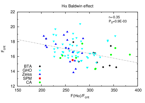
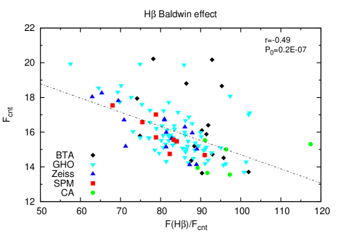
Figure 6: Baldwin effect in the H$\alpha$ (upper) and H$\beta$ line (bottom). The continuum flux is in units $10^{-16}\rm erg\ cm^{-2}s^{-1}\AA^{-1}$. Observations with different telescopes are denoted with different symbols given in the bottom left. The correlation coefficient and the corresponding p-value are also given.

In Figs. 4 and 5 we plot the H$\beta$ and H$\alpha$ line fluxes as a function of the continuum. Since the observations with Zeiss should be taken with caution, we present the line vs. continuum flux with and without data obtained with Zeiss (see Tables 1 and 2, code Z2K). As it can be seen from figures, there is a relatively week correlation between the line and continuum fluxes, r=0.42 for H$\beta$ and 0.42 for H$\alpha$ (without Zeiss data). Such small correlation between the line and the continuum flux also indicates that beside the continuum central source there may be present other effects in photoionization.

On the other hand in Fig. 6 we plot the intrinsic Baldwin effect, and as it can be seen there is an anticorrelation between the continuum flux and equivalent widths of the H$\beta$ ($r=-0.49,P_{0}=0.6\cdot 10^{-07}$) and H$\alpha$ lines ($r=-0.35,P_{0}=0.9\cdot 10^{-03}$), i.e. that there is the intrinsic Baldwin in the H$\beta$ and H$\alpha$ lines, similar as it is observed in another (single peaked) AGNs (see e.g. Gilbert & Peterson, 2003).

We defined the observed fluxes in the blue and red wings, and in the core of the H$\alpha$ and H$\beta$ lines (Tables LABEL:tab_seg_ha-LABEL:tab_seg_hb) in the wavelength intervals as they are given in Table 5. In Fig. 7 we plot the H$\alpha$ and H$\beta$ line-wing fluxes (blue, red) vs. line-core flux (upper panels), and red vs. blue-wing (bottom panel). The dashed line in Fig. 7 represents the best fit, while the solid line represents the expected slope in the case that the different parts of the line profile vary proportionally to each other, i.e. the slope of the best fit is 1.

As it can be seen in Fig. 7 the correlations in variation between the blue/red wings and central component are high, as well as between the red and blue wings ($r\sim 0.8$). However, the slopes of the best-fit lines are not consistent with 1, except in the case of H$\beta$ red wing vs. core, where the best fit is very close to 1.

Although the correlations between the H$\alpha$ vs. H$\beta$ total line and line segment fluxes (Fig. 9) are very good ($r\sim 0.8$), the best fits are far away from the slope of 1. Moreover, in the case of the line cores, F(H$\alpha)$core vs. F(H$\beta$)core, the correlation coefficient is smaller ($r\sim 0.65$). On the other hand, the correlation between the line segment and continuum flux is very low, i.e. almost absent and statistically not important in the case of H$\alpha$ (see Fig. 8). The situation is slightly better in the case of the H$\beta$ line.

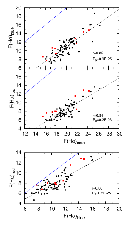
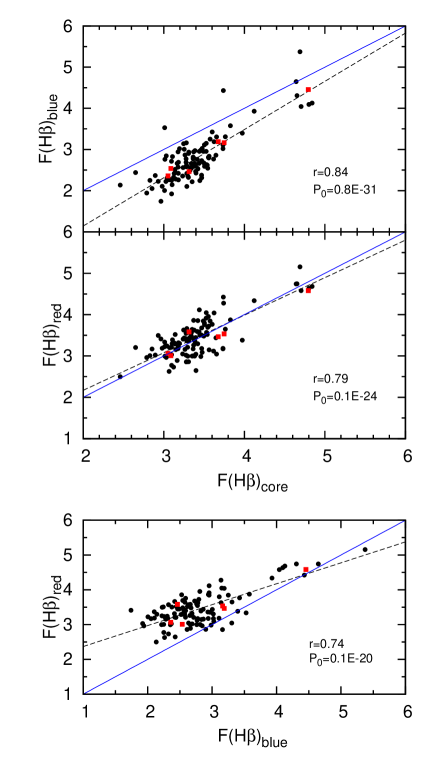
Figure 7: H$\alpha$ and H$\beta$ line-wing fluxes (blue, red) vs. line-core flux (upper panels), and red vs. blue-wing (bottom panel). The line-segment fluxes are in units $10^{-14}\rm erg\ cm^{-2}s^{-1}$. The correlation coefficient and the corresponding p-value are given in the bottom right corner. The CA-data are denoted with squares. The dashed line gives the linear best-fitting of the data, while the solid line markes the linear function with the slope equals to 1.

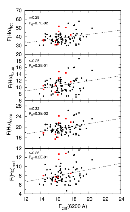
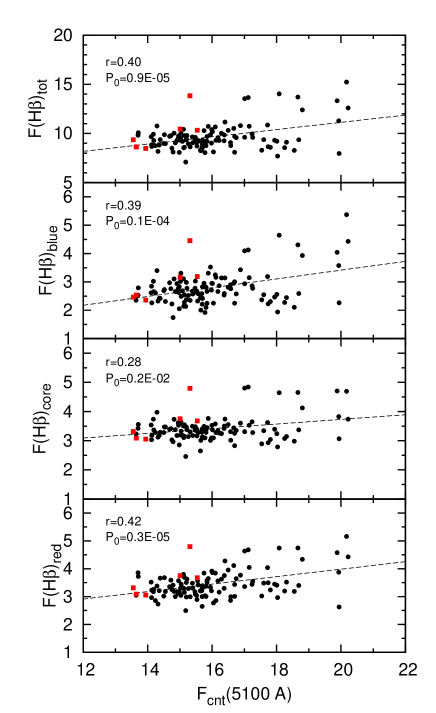
Figure 8: H$\alpha$ and H$\beta$ line and line-segment fluxes (blue, core and red) vs. continuum flux at 6300 and 5100, respectively. The continuum flux is in units $10^{-16}\rm erg\ cm^{-2}s^{-1}A^{-1}$, and the line-segment fluxes are in $10^{-14}\rm erg\ cm^{-2}s^{-1}$.The correlation coefficient and the corresponding p-value are given in the upper left corner. The CA-data are denoted with squares.

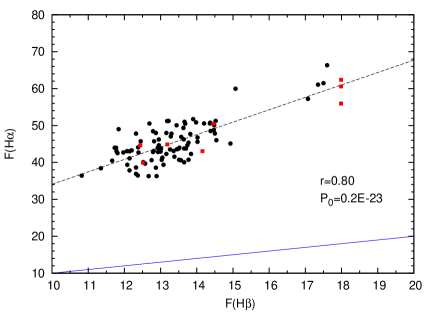
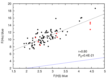
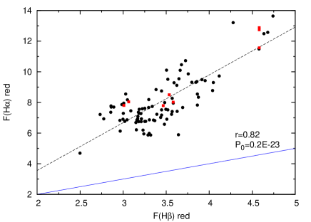
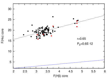
Figure 9: H$\alpha$ vs. H$\beta$ total line and line segment fluxes (blue, red, core). The correlation coefficient and the corresponding p-value are given in the bottom right corner. The CA-data are denoted with squares. The dashed line gives the linear best-fitting of the data, while the solid line markes the linear function with the slope equals to 1.

Table 13: Sampling characteristics and cross-correlation analysis of H$\beta$.

Light curve	N	Lag ZDCF	ZDCF
cnt vs H${\alpha}$	79	$14.94_{-13.81}^{15.66}$	$0.19_{-0.14}^{0.14}$
cnt vs H${\alpha}$ (bad Zeiss discarded)	60	$16.29_{-14.34}^{14.30}$	$0.28_{-0.16}^{0.15}$
cnt vs H${\beta}$	110	$20.61_{-18.71}^{54.33}$	$0.31_{-0.09}^{0.09}$
cnt vs H${\beta}$ (only Mexico points)	80	$10.75_{-9.76}^{19.31}$	$0.15_{-0.13}^{0.13}$
cnt vs H${\beta}$ (without Zeiss)	95	$16.85_{-14.86}^{20.13}$	$0.34_{-0.11}^{0.10}$

3.1.1 CCF analysis

As it can be seen, the light curves shown in Fig. 3 are complex, with a number of peaks, and the observed fluxes show only modest indications for variations, which is indicated by F(var) parameter in Table 10. In spite of the small correlation between the line and continuum fluxes, we apply on our data-samples the Z-transformed DCF method, called ZDCF (see Alexander, 2013). We did several calculations, using different number of data, first of all, we discarded bad Zeiss spectra, also we calculated CCF using only spectra observed with two telescopes from Mexico. The results of the cross-correlation analysis are given in Table 13.

It could be seen that the continuum and both line emission light curves H${\alpha}$ and H${\beta}$ (without bad Zeiss spectra) varies similarly. As it can be seen from Table 13, the lags for H$\beta$, for different number of points, are between 20 and 29 days, and for H$\alpha$ between 17 and 29 days. The cross correlations are small, but the ZDCF coefficient is larger in the case of H${\beta}$.

Additionally, we apply the method of Zu et al. (2011) for the lag estimation of the H$\beta$ line (Fig. 10). We also applied this method on the H$\alpha$ line, however, it did not produce valid results. In these calculations, the first step is to build a continuum model to determine the Zu model parameters of the continuum light curve. The continuum light curve is generated from the model with the time scale of 100 days and variability amplitude of $\sigma=2$. The posterior distribution of the two parameters of the continuum variability $(\tau_{d},\sigma)$ are calculated from Zu model using 40000 MCMC (Markov Chain Monte Carlo) method burn-in iterations. In order to measure the lag between the continuum and the H$\beta$ light curve, Zu model then interpolates the continuum light curve based on the posteriors $(\tau_{d},\sigma)$ derived, and then shifts, smooths, and scales continuum light curve to compare to the observed H$\beta$ light curve. After doing this 10000 times in an MCMC run, we derived the posterior distribution of the lag, the tophat width w, and the scale factor s of the emission line, along with updated posteriors for the timescale $\tau_{d}$ and the amplitude $\sigma$ of the continuum. The model gives for lag between continuum and H$\beta$ line $36.95_{19.72}^{47.53}$ days and for continuum and H$\alpha$ line the lag is $22.86_{16.84}^{30.20}$ days which is approximately within 3$\sigma$ distance from lag values between continuum and emission lines obtained by classical methods given in Table 13. In order to know what the best fitting parameters from the last MCMC run look like, we give in Fig. 10 a comparison of the best-fitting light curves and the observed ones. It could be seen that the observation between MJD 46975 and 50991 are closer to the best-fitting light curve in the case of H$\alpha$ than in the case of the H$\beta$ line.

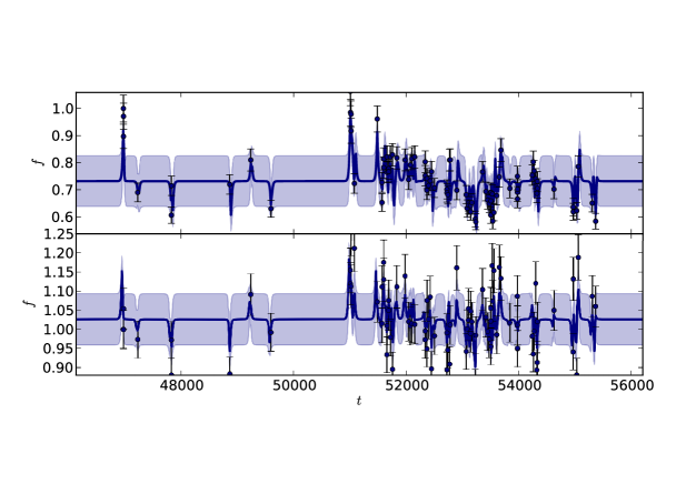
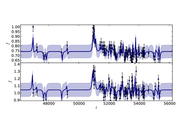
Figure 10: Models of H$\alpha$ (up) and H$\beta$ line (down), where the upper panel gives the line and the bottom panel continuum light curve. On all plots full line is the model of the expected mean light curve, while dots represent the observed data. The blue band shows the expected spread of light curves around the mean consistent with the data. The x-axis gives modified Julian Date (MJD) while the y-axis gives normalized line/continuum fluxes.

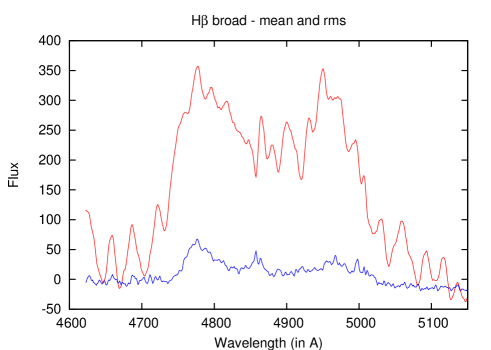
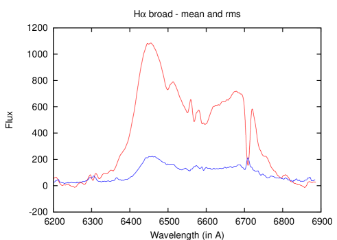
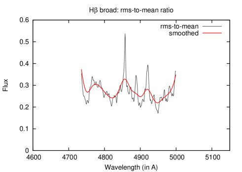
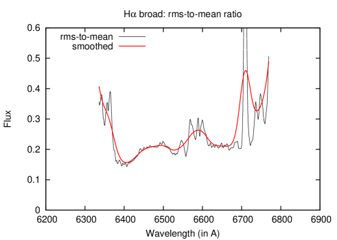
Figure 11: Top panels give the mean and rms profiles, while the bottom panels give the ratio of the rms-to-mean flux of the H$\beta$ (left) and H$\alpha$ (right) lines.

Finally, we applied the interpolation cross-correlation function method (ICCF) method (Bischoff & Kollatschny, 1999) to cross-correlate the flux of the continuum with H$\beta,\alpha$ flux. Also in this case, the error-bars in lags were large and there is an indication for a lag of 20 days, that is in agreement with previous two methods. Therefore, for the black hole mass estimation we will accept a time lag for H$\beta$ of 20 days.

3.2 Changes in the broad line profiles

We are going to discuss and model the line shapes variability in Paper II, here we will give some characteristics of the line profile and peaks variations, since Arp 102B is a prototype of double peaked emitters.

During the monitoring period, the broad H$\beta$ and H$\alpha$ lines have double-peaked profiles. In Fig. 11 we present the mean profile accross the line profile H$\beta$ and H$\alpha$ profiles and their rms profile (top panels) and normalized rms on the mean profile across the line profile (bottom panels). The FWHM of the mean and rms profiles are: H$\alpha$ mean 14,320 km s^-1 and rms 14,450 km s^-1, and H$\beta$ mean 15,900 km s^-1 (15,840 km s^-1) and rms 14,870 (or 16,080 if not corrected for the underlying continuum). The distance between the two peaks is around 11,000 km s^-1, the blue peak is located around -5,000 km s^-1 and red around 6,000 km s^-1 from the line center. Such big distances between the peaks indicate a fast rotating disk, that is probably close to the black hole. As it can be seen from Fig. 11, the changes in the line profile have also two peaked rms, that indicates that the changes in the broad line profile are in both red and blue peak in both lines, but changes in the blue wing are significantly bigger, than in the red one. Note here, that there is one, central, peak in the rms, that may be caused by a central component (see e.g. Popović et al., 2004; Bon et al., 2006, 2009).

3.2.1 Red to blue peak ratio

As it was reported in Newman et al. (1997) and Sergeev et al. (2000) there is the variation in the red-to-blue flux ratio of H$\alpha$ that has a periodical characteristic. The observed wavelength intervals of H$\alpha$ are defined in such a way that the red wing excludes the narrow forbidden lines of [N II]$\lambda$6584 and [S II] $\lambda\lambda$6717,6731 (H$\alpha$ - red1 and H$\alpha$ - red2 from Table 5). The blue and red wavelength intervals (see Table 5) correspond to intervals from Newman et al. (1997) in case of H$\alpha$. We measure the line-segment flux ratio for H$\alpha$ and H$\beta$ (Tables LABEL:tab_seg_ha – LABEL:tab_seg_hb, available electronically only) and apply the so called Lomb-Scargle periodogram (Lomb, 1976; Scargle, 1982) to find possible periodical variations in this ratio.

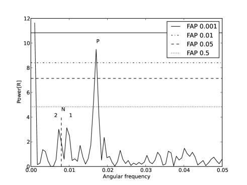
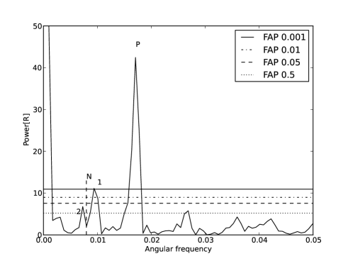
Figure 12: Left: Lomb Scargle periodograms of the ratio of the red-to-blue line-segment fluxes $R$ of H$\alpha$ (left) and H$\beta$ (right) lines (false-alarm probability (FAP) lines are also indicated).

Fig. 12 gives the Lomb Scargle periodograms of the ratio of the red-to-blue line-segment fluxes ($R$=$F$(red)/$F$(blue)) of the H$\alpha$ and H$\beta$ lines. As it can be seen in Fig. 12 there are three peaks, where one peak is clearly distingueshed and higher than 0.01 (99%) of false-alarm probability (FAP). This peak (denoted as P-peak) at angular frequency of $\sim$0.017 in case of both lines, corresponds to the period of $\sim$370 days. The angular frequency of 0.00795 corresponding to the period of $\sim$790 days found by Newman et al. (1997) and Gezari et al. (2007) (denoted with N), seems to be located between two other peaks of lower significance (denoted as 1- and 2-peak in Fig. 12): the 1-peak is at angular frequency of $\sim$0.00968 for H$\alpha$ (0.0094 for H$\beta$) corresponding to the period of $\sim$650 days (670 days), and the second peak is at angular frequency of $\sim$0.0074 (0.0077) corresponding to the period of $\sim$850 days (815 days).

4 Discussion

Here we discuss our results, but before that, we should point out that the host-galaxy of Arp 102b is an E-galaxy with strong stellar absorption lines (Mg Ib,Na ID, CaII H,K etc.) typical for this type of galaxies. The host galaxy contininuum can strongly affect the observed spectra, therefore we determined the host-galaxy contribution to the blue and red fluxes of the observed continuum as well as to the H$\alpha$, H$\beta$ emission line fluxes (given in absolute units, see Table 8). To estimate the host galaxy continuum contribution, we used Arp 102b and NGC 4339 (E0) spectra observed in the same night under the same good weather conditions (see §2.4). To subtract the NGC 4339 galaxy spectrum from Arp 102B one, we use Mg Ib, and found that the best fit (when the Mg1b and Na ID are completely removed from the composite spectra) is with a 75$\pm$3% of the host-galaxy contribution to the total Arp 102B continuum at $\sim$5100 Å in the considered spectrum. However, depending on AGN activity phase, the host galaxy contribution to the continuum at $\sim$5100 Å was between $\sim$ 60% and $\sim$ 80% in the monitoring period.

Additonally, we estimated the narrow line contributions to the total and line-segment fluxes of H$\alpha$ and H$\beta$ (see Table 9). Consequently, further in the discussion we will point out the parts where these contributions are improtant.

4.1 Variation of the broad lines and continuum

As it can be seen in Fig. 3 the broad line and continuum fluxes change for 10-30% during the monitoring period (1987–2010). Some flares with amplitude of $\sim$(10-20)% are observed, and these are especially strong in H$\alpha$ and continuum. The flare like variation of Arp 102B was noted in Gezari et al. (2007).

Actually, in 1987 (from Jun28 – JD2446975 to Jun30 – JD2446977), and in 1998 (from May6 – JD2450940 to Jul26 – 2451021) there has been a rise in the observed flux of the H$\alpha$ and H$\beta$ emission lines of 30-40%, in the form of a flare-like event with duration of about 80 days in 1998, but in the continuum such strong oserved flux changes were not observed. In Table 12 we obtain that the different observed mean line fluxes between 1987 and 1988–1994, and also between 1998 and 1999–2010 changed significantly, more than the continuum fluxes 32–35% in H$\beta$ and $\sim$(38–39)% in H$\alpha$, compared to 6–13% and 7–19% in the red and blue continuum, respectively.

However, after the host-galaxy contribution subtraction we obtained that in the same (above noted) periods the relative amplitude of the variability of the mean corrected continuum (i.e. agn-continuum) is significantly larger: 1987/(1988–1994)$\sim$1.3 and 1998/(1999–2010)$\sim$1.6 than it was in the host galaxy+agn continuum: 1987/(1988–1994)$\sim$1.07 and 1998/(1999–2010)$\sim$1.19–1.13. These variations are comparable with relative line flux variations.

A similar result was obtained for the parameter F(var) - the variation amplitude of fluxes with respect to the mean flux (Table 10, host-galaxy corrected data). As seen from Table 10, F(var) in the corrected continuum fluxes (in agn-continuum) has a significantly larger continuum variability amplitude, than the observed total continuum (for continuum at 5100A: 31% against $\sim$9% in non-corrected spectra; for continuum at 6200A: 29% against $\sim$7% in non-corrected spectra). On the other hand, F(var) in the H$\alpha$ and H$\beta$ lines, after removing the contribution of the host-galaxy, remaineds almost unchanged (see host galaxy corrected data in Table 10). In the corrected blue and red continuum there are some possible flares of amplitude up to 30% with a duration of a few (2-3) days (see Table 11), but these flares are not detected in the corrected H$\alpha$ and H$\beta$ line fluxes.

As noted above, we observed strong changes of mean fluxes in the corrected continuum in almost constant changes mean flux in the broad lines i.e. greatly reduced mean continuum flux (in 1.3 times to in 1988–1994 and 1.6 times in 1999–2010) while changes in the broad line fluxes remaine at the same level (1.3 times). The amplitude of variability of the continuum and line fluxes stays closer each other, when we corrected the line fluxes for the narrow line contributions, but a small correlation between the agn-continuum and line fluxes remains (see Fig. 9).

Additionally, we should note that small amount of the optical continuum emission may not be too effective in the broad line reproduction. As e.g. Chen et al. (1989) have shown that the gravitational energy liberated in a standard accretion disk is not much larger than the observed line emissivity in Arp 102B, so an extra source of heating possibly may be required. They hypothesize that ion-supported tori might account for the unusual properties of Arp 102B. On the other hand the amplitude of variability of the optical continuum is comparable with the line one. Additionally, there may be situation that the amplitude of variability and intensity of the far UV and X-ray contina is even strong for driving of the line variability and intensity. Also, it is well known (see e.g. Vagnetti, et al., 2013) that the variability of the high-energy bands (as X-ray) often is more pronounced that the variability of the UV/optical band. But the question of the weak correlation between the continuum and line fluxes remains.

The most interesting result is the almost lack of correlation between the continuum and broad lines (r$\sim$0.31, see Fig. 4 and Fig. 5) We obtained delays between H$\alpha$ and H$\beta$ emission line fluxes and continuum flux (lags $\sim$15-20 days), see Table 13, using different CCF methods. However the errors in lags are huge due to the fact that the flux variability in both lines and continuum during the monitoring period was small ($\sim$10-20%, see Table 10). Note here that in the case of AGNs with very broad lines, the lag calculation is difficult (see e.g. the cases of NGC7603 and Mrk926 in Kollatschny et al., 2000; Kollatschny & Zetzl, 2010, respectively). The weak correlations between the line and continuum fluxes and non-confidently lags-data indicate also a possible another sources of photoionization in the BLR except the central source (e.g. collisions of orbiting discrete clouds in disk (Sergeev et al., 2000))

Additionally, similar as in some single peaked AGNs (see e.g. Gilbert & Peterson, 2003), the H$\beta$ and H$\alpha$ lines show intrinsic Baldwin effect, or significant anticorrelation between the continuum flux and equivalent widths of broad lines (see Fig. 6). The anticorrelation tends to be stronger in H$\beta$ (and statistically more significant) than in the H$\alpha$ line.

4.2 Black hole mass in Arp 102B

Mostly, reverberation calculations have been applied on the cases which give black hole masses within the range $10^{7}-10^{9}M\odot$. Up to now, emission-line lags have been measured for a number of AGNs by using the cross correlation between the continuum and emission-line light curves.

Using the virial theorem, the mass of black hole ($M_{BH}$) is (Peterson et al., 1998; Wandel et al., 1999):

$$M_{GRAV}=f{\Delta V_{FWHM}\cdot R_{BLR}\over G},$$

where $\Delta V_{FWHM}$ is the orbital velocity at that radius $R_{BLR}$ of the BLR, and it is estimated by the width of the emission line (specifically, the variable part of the line); the $f$ is the factor that depends on the geometry of the BLR. Using a sample disk model for the Arp 102B BLR, one can use the relation givne in Onken et al. (2004):

$$M_{BH}=f{\Delta V_{FWHM}\cdot R_{BLR}\over G}\cdot{\sin(i)\over{2\ln(2)}},$$

where $i$ is the inclination of the disk. Here we take $f=5.5$ as estimated by Onken et al. (2004) and $i\sim 30^{\circ}$ as given in Chen & Halpern (1989).

The velocity dispersion of the disk can be estimated as (see La Mura et al., 2009)

$$\Delta v={FWHN(H\beta)\over{8\sin(i)}},$$

where for our measurements $v_{\rm FWHM}({\rm rms})\approx 15000$ km s^-1 (Fig 11b) and $i\sim 30^{\circ}$ gives $\Delta v=3750\rm\,km\,s^{-1}$. Taking into account that our estimate is $R_{BLR}\approx 20$ light days (Table 13), we obtaine a mass of the Arp 102B black hole to be $\sim 1.1\cdot 10^{8}M_{\odot}$.

There are other estimates of the BH mass in Arp 102B; using the hot spot model for the explanation of the variations of the line profile, Newman et al. (1997) estimated the black hole mass in Arp 102B to be $2.2\times 10^{8}M_{\odot}$, while from the rotational clouds model, Sergeev et al. (2000) estimated the central body mass of $3.5\times 10^{8}M_{\odot}$.

It is interesting to compare the obtained BH masses mentioned above with $M-\sigma*$ relation. Recently, the $M-\sigma*$ relation was given by Gültekin et al. (2009) as:

$$\log(M_{BH}/M_{\odot})=\alpha+\beta\log(\sigma*/200{\rm km\ s^{-1}})$$

where $\alpha=(8.12\pm 0.08$ and $\beta=4.24\pm 0.41$ are constants, and $\sigma*$ is the stellar disspersion. The disperssion velocity for Arp 102B was given by Barth et al. (2002) as $\sigma_{*}=188\pm 8\ \rm km\ s^{-1}$ that gives an estimated Arp 102B black hole mass as $M_{BH}\sim 1.01\cdot 10^{8}M\odot$.

Comparing the data obtained from our estimates, as well as estimates of Newman et al. (1997) and Sergeev et al. (2000), the $M-\sigma*$ relation gives a smaller mass for Arp 102B than estimated by Newman et al. (1997) and Sergeev et al. (2000) (two and three times, respectively). However, comparing our results and that obtained from $M-\sigma_{*}$ relation the agreement is very good $M_{rev}/M_{M-\sigma*}\sim 1.1$.

The black hole masses of AGNs with double-peaked lines obtained with $M-\sigma_{*}$ relation seem to disagree systematically with the virial masses obtained from one epoch measurements (see Wu & Liu, 2004; Lewis & Eracleous, 2006). But it seems that the revereberation method gives better agreement, that is the case in another double-peaked AGN, 3C390.3, namely Dietrich et al. (2012) found that in the case of double-peaked line emitter 3C390.3 the reverberation based mass of the BH also agrees with $M-\sigma_{*}$ relations.

4.3 H$\alpha$ and H$\beta$ flux variability

We explored changes in the total line fluxes of H$\alpha$ and H$\beta$ as well as in the line segments (see Table 5). There are changes in the line profiles (blue and red double peaks, see §3.4) and their rms. The observed line parts in both lines are varying around $\sim$20% (see Table 10). The correlations between the line segments are significant, however the slopes of the best fit are not are not consistent with one, only in the case of the H$\beta$ red wing vs. the H$\beta$ line core the slope follows of 1 (see Fig. 7).

As seen from Fig. 8 there is only a weak correlation between fluxes of different segments of both lines and continuum flux (r$\sim$0.3–0.4). However, we find a very good correlation (r$\sim$0.8) between the H$\alpha$ and H$\beta$ (for total line and for line-segment fluxes, see Fig. 9), and between the fluxes of the blue, red, and core segments of the H$\alpha$ and H$\beta$ (Fig. 7), that is in agreement with the disk geometry.

On the other hand, we found an indication of periodical changes in the peak ratio (i.e. red-to-blue line-segment flux ratio), with the period of around 370 days, that is smaller than the period obtained by Newman et al. (1997) and Gezari et al. (2007). However, we found two peaks in the periodogram very close to the period obtained by Newman et al. (1997) (with lower significance, especially for the H$\alpha$ line where the peaks are below 50% of the false-alarm probability line). Newman et al. (1997) pointed out that the determined period seems to be an orbital motion through the evolution of the ratio of red to blue fluxes (or, alternatively, through the evolution of parameter $\theta$, the azimuthal angular extent of the hot spot, in the models). Also Gezari et al. (2007) interpreted the observed oscillation as two different bright spots orbiting at different radii in the disk at different times, but the authors mentoined the problem with this model, since the two bright spots rotation periods did not yield consistent values of the black hole mass. However, such a scenario – two different bright spots orbiting at different radii – successfully explains the line shape variability in the case of 3C390.3 (see Jovanović et al., 2010).

Indeed, the only proposed source of variability in an AGN, that would cause simple periodical sinusoidal variation in this ratio with little apparent decay (in amplitude or frequency) for nearly two complete cycles, is orbital in nature. But, the problem here is that there are indications for three possible rotation period (two with lower significance close to period given in Newman et al., 1997, and one that is almost two times smaller).

Alternativelly, it is possible that the rotation of the bright spot in the accretion disk is not pure Keplerian; the bright spot, as e.g. may be affected by a wave in the disk that rotates at a different speed (see Lewis et al., 2010). This may be an explanation for multi-periodical oscillations seen in the spectra of Arp 102B, but this we will consider in more details in the forthcoming paper.

5 Conclusion

Here we present a long term (1987–2010) spectroscopical observations of Arp 102B in the optical band, an AGN with prominent double-peaked broad line profiles. We investigated the continuum and line variations during this period and from our investigations we can outline the following conclusions:

i) We found a significant contribution the host-galaxy continuum (between $\sim$ 60% and $\sim$ 80% in the monitoring period) to the total observed continuum in Arp 102B. The corrected (agn) continuum flux of Arp 102b approximately has a flat shape and it contributes around $\sim$25% to the total observed (host+agn) continuum (Fig. 1, bottom). The flux variation of the agn-continuum has a significantly larger amplitude than it can be seen in the observed total continuum (Table 10, F(var)). However, the H$\alpha$ and H$\beta$ line fluxes are not sensitive to the host-galaxy correction, i.e. the variability amplitude remains almost unchanged (Table 10). As noted in §3, the corrected AGN continuum shows some possible flare-like events, i.e. an increase in the flux up to $>30$ % within a few (2-3) days (see Table 11), but correspond flare-like events were not observed in the broad H$\alpha$ and H$\beta$ light curves.

ii) In different parts of the monitoring periods, mean observed fluxes of the H$\alpha$, H$\beta$ broad emission lines and blue/red continuum variations are small (5-10%, Table 10). But changes of the different mean fluxes in the lines between 1987 and (1988–1994), and between 1998 and (1999–2010) are significantly larger than changes of continuum fluxes. However, after subtracting the host-galaxy contribution (in the the same periods) the amplitude of changes of the mean continuum fluxes (i.e. agn-continuum) is significantly larger (1987/(1988–1994)$\sim$1.3 and 1998/(1999–2010)$\sim$1.6). After removing the narrow line contribution the line flux amplituda variation, the relative AGN continuum changes are comparable (or even greater) with the flux changes in lines. A rise in the H$\alpha$ and H$\beta$ emission line fluxes about 30–40% in 1987 and 1998 is similar to a long flare duration of about 80 days in 1998 (in 1987 observations are only 3 days). However the mean fluxes during single years 1987, 1998 and during periods 1988–1994 and 1999–2010 are constant inside this periods within 5-10% errorbars (Table 12).

iii) The correlations between the observed fluxes of the H$\alpha$ and H$\beta$ lines, as well as of their line segments, with continuum fluxes (Figs. 4-5) is very weak (r$\sim$0.3–0.4). That points to additional sources of ionization in the BLR apart from the central AGN continuum source. But there is a good linear relation between the observed fluxes in different line segments (r$\sim$0.8), i.e. between blue and red wings, and line core (Fig. 7), and between the H$\alpha$ and H$\beta$ (Fig. 9) for total line and line segment fluxes, that indicates the same geometry for both emission regions. Also the anticorrelation between the continuum flux and equivalent widths of the H$\alpha$ and H$\beta$ lines (intrinsic Baldwin effect) is observed (r$\sim$0.37 for H$\alpha$, r$\sim$0.49 for H$\beta$, see Fig. 6), as in some Seyfert galaxies (Gilbert & Peterson, 2003).

iv) During the monitoring period, the broad H$\alpha$ and H$\beta$ lines of Arp 102B show double-peaked profiles. The blue peak is located around -5,000 km s^-1 and red around 6,000 km s^-1 from the line center. A big distance between the peaks ($\sim$ 11,000 km s^-1) indicates a fast rotating disk, that is probably close to the black hole. As it can be seen from Fig. 11 (mean profiles and rms), the changes in the line profile have also double-peaked rms, that indicates that changes in the blue wing is significantly (some) bigger, than in the red wing. In the rms there is one central peak, that may be caused by a central component in the BLR (Popović et al., 2004; Bon et al., 2006, 2009).

v) From the Lomb-Scargle periodogram method, applied on the measured red-to-blue peak flux ratio ($R$=$F$(red)/$F$(blue)) of H$\alpha$ and H$\beta$ lines, we found possible periodical variations (signals) in this ratio. We found a period of around 370 days, and two additional peaks close to the period found by Newman et al. (1997).

vi) Several cross-correlation methods of the continuum and H$\alpha$, H$\beta$ broad emission line fluxes indicates a lag of $\sim$15-20 days with large errorbars, caused by the small flux variations in period monitoring and not so good data sampling.

vii) From mean and rms profiles both emission lines we found FWHM(rms)$\sim$15,000 km s^-1 and from the CCF analysis we obtained a lag$\sim$20 days, thus we estimated the reverberation central black hole mass of $M_{\rm rev}\sim 1.11\times 10^{8}M_{\odot}$, that is smaller than previous estimates (Newman et al., 1997; Sergeev et al., 2000), but is in an agreement with estimated black hole mass obtained from the $M-\sigma*$ relation.

The main property of the double-peaked Seyfert galaxy Arp 102B is the long-term variability on the timescale of months to some years, which is consistent with the dynamical timescale of an accretion disk. The observed long flare in H$\alpha$ and H$\beta$ with the duration of about 80 days in 1998 cannot be only due to the ionization by the AGN-continuum source. Also, due to the lack of correlations with the AGN-continuum this variability can be attributed to inhomogeneities in the line-emitting disk, i.e., hot spots, spiral arms, eccentricity, and warps. We will consider in more details the nature of the broad spectral shape variability and consequently the BLR geometry in the forthcoming Paper II.

References

- Alexander (2013) Alexander, T, 2013, http://adsabs.harvard.edu/abs/2013arXiv1302.1508A
- Antonucci et al. (1996) Antonucci, R., Hurt, T., Agol, E. 1996, ApJ, 456, L20
- Barth et al. (2002) Barth, A. J., Ho, L. C., Sargent, W. L. 2002, AJ, 124, 2607
- Bischoff & Kollatschny (1999) Bischoff, K., & Kollatschny, W. 1999, A&A, 345, 49B
- Bon et al. (2009) Bon, E., Popović, L. Č., Gavrilović, N., La Mura, G., & Mediavilla, E. 2009, MNRAS, 400, 924
- Bon et al. (2006) Bon, E., Popović, L., Ilić, D., Mediavilla, E. 2006, NewAR, 50, 716
- Chen & Halpern (1989) Chen, K. & Halpern, J. 1989, ApJ, 344, 115
- Chen et al. (1989) Chen, K. Halpern, J. P., Filippenko, A. V. 1989, ApJ, 339, 742
- Chen et al. (1997) Chen, K, Halpern, J. P., Titarchuk, L. G. 1997, ApJ, 483, 194
- Dietrich et al. (2012) Dietrich, M., Peterson, B. M., Grier, C. J. et al. 2012, ApJ, 757, 53
- Dimitrijević et al. (2007) Dimitrijević, M. S., Popović, L. Č., Kovačević, J., Dačić, M., Ilić, D. 2007, MNRAS, 374,1181
- Eracleous & Halpern (1994) Eracleous, M., & Halpern, J. P. 1994, ApJS, 90, 1
- Eracleous et al. (1997) Eracleous, M., Halpern, J., Gilbert, A., Newman, J. A., Filippenko, A.V. 1997, ApJ, 490, 216
- Eracleous et al. (2009) Eracleous, M., Lewis,, K.T., Flohic, H. M.L.G. 2009, NewAR, 53, 133
- Fathi et al. (2011) Fathi, K., Axon, D. J., Storchi-Bergmann, T., Kharb, P., Robinson, A., Marconi, A., Maciejewski, W., Capetti, A. 2011, ApJ, 736, 77
- Flohic & Eracleous (2008) Flohic, H. M. L. G., Eracleous, M. 2008, ApJ, 686, 138
- Gaskell (2009) Gaskell, C. M. 2009, NewAR, 53, 140
- Gilbert & Peterson (2003) Gilbert, K. M., Peterson, B. M. 2003, ApJ, 587, 123
- Gezari et al. (2007) Gezari, S., Halpern, J. P., & Eracleous, M. 2007, ApJS, 169, 167
- Gezari et al. (2004) Gezari, S., Halpern, J. P., Eracleous, M., Filippenko, A. V. 2004, IAUS, 222, 95
- Gültekin et al. (2009) Gültekin, K., Richstone, D. O., Gebhardt, K. et al. 2009, ApJ, 698, 198
- Halpern et al. (1996) Halpern, J. P., Eracleous, M., Filippenko, A. V., & Chen, K. 1996, ApJ, 464, 704
- Jovanović et al. (2010) Jovanović, P., Popović, L. Č., Stalevski, M., Shapovalova, A. I. 2010, ApJ, 718, 168
- Kollatschny et al. (2000) Kollatschny, W., Bischoff, K., Dietrich, M., 2000, å, 361, 901
- Kollatschny & Zetzl (2010) Kollatschny, W., & Zetzl, M. 2010, A&A, 522, A36
- La Mura et al. (2009) La Mura, G., Di Mille, F., Ciroi, S., Popović, L. Č., Rafanelli, P. 2009, ApJ, 693, 1437
- Lewis & Eracleous (2006) Lewis, K. T., Eracleous, M. 2006, ApJ, 642, 711
- Lewis et al. (2010) Lewis, K. T., Eracleous, M., Storchi-Bergmann, T, 2010, ApJS, 187, 416
- Lomb (1976) Lomb, N.R., 1976, Ap&SS, 39, 447
- Miller & Peterson (1990) Miller, J. S., Peterson, B. M. 1990, ApJ, 361, 98
- Newman et al. (1997) Newman, J. A., Eracleous, M., Filippenko, A. V., Halpern, J. 1997, ApJ, 485, 570
- O’Brien et al. (1998) O’Brien P.T., Dietrich, M., Leighly, K et al. 1998, ApJ, 509, 163
- Onken et al. (2004) Onken, C. A., Ferrarese, L., Merritt, D., Peterson, B. M., Pogge, R. W., Vestergaard, M., Wandel, A., 2004, ApJ, 615, 645
- Peterson (1993) Peterson, B. M. 1993, PASP, 105, 207
- Peterson et al. (1998) Peterson, B. M., Wanders, I., Bertram, R., et al. 1998, ApJ, 501, 82
- Peterson et al. (1999) Peterson, B. M., Barth, A. J., Berlind, P., et al. 1999, ApJ, 510, 659
- Peterson et al. (1994) Peterson, B. M., Berlind, P., Bertram, R., et al. 1994, ApJ, 425, 622
- Peterson et al. (2002) Peterson, B. M., Berlind, P., Bertram, R., et al. 2002, ApJ, 581, 197
- Peterson & Collins (1983) Peterson, B.M., & Collins II, G.W. 1983, ApJ,270,71
- Peterson et al. (1995) Peterson, B. M., Pogge, R. W., Wanders, I., Smith, S. M., & Romanishin, W. 1995, PASP, 107, 579
- Popović et al. (2004) Popović, L. Č., Mediavilla, E., Bon, E., & Ilić, D. 2004 A&A 423, 909
- Popović et al. (2001) Popović, L. Č.. Mediavilla, E. G., Muñoz, J. A.2001, A&A, 378, 295
- Popović et al. (2011) Popović, L. Č., Shapovalova, A. I., Ilić, D. et al. 2011, A&A, 528A, 130
- Scargle (1982) Scargle, J.D., 1982, ApJ, 263, 835
- Shapovalova et al. (2001) Shapovalova, A. I., Burenkov, A. N., Carrasco, L., et al. 2001, A&A, 376, 775
- Shapovalova et al. (2004) Shapovalova, A.I., Doroshenko, V.T., Bochkarev, N.G, et al. 2004, A&A, 422, 925
- Shapovalova et al. (2010) Shapovalova, A. I., Popović, L.Č., Bochkarev, N.G., et al. 2010, A&A, 517A, 42
- Shapovalova et al. (2009) Shapovalova, A. I., Popović, L.Č., Bochkarev, N.G., et al. 2009, NewAR, 53, 191
- Shapovalova et al. (2012) Shapovalova, A.I., Popović, L.Č., Burenkov, A. N., et al. 2012, ApJS, 202, 10
- Shapovalova et al. (2008) Shapovalova, A.I., Popović, L.Č., Collin, S., et al. 2008, A&A, 486, 99
- Sergeev et al. (2000) Sergeev, S. G., Pronik, V. I., Sergeeva, E. A. 2000, A&A, 356, 41
- Stauffer et al. (1983) Stauffer, J., Schild, R., Keel, W. 1983, ApJ, 270, 465
- Sulentic et al. (2000) Sulentic, J. W., Marziani, P., Dultzin-Hacyan, D.2000, ARA&A, 38, 521
- Sulentic et al. (1990) Sulentic, J. W., Zheng, W., Calvani, M., Marziani, P. 1990, ApJ, 355, 15
- van Groningen & Wanders (1992) Van Groningen, E. & Wanders, I. 1992, PASP, 104, 700
- Vagnetti, et al. (2013) Vagnetti, F.; Antonucci, M., Trevese, D.Veron, P., 2013, A&A, 550A, 71
- Wandel et al. (1999) Wandel, A., Peterson, B. M., & Malkan, M. A. 1999, ApJ, 526, 579
- Wu & Liu (2004) Wu, X.-B., Liu, F. K. 2004, ApJ, 614, 91
- Zu et al. (2011) Zu, Y., Kochanek, C. S., Peterson, Bradley M. 2011, ApJ, 735, 80.